*

Abstract

This paper considers ideal gas-like models of trading markets, where each agent is identified as a gas molecule that interacts with others trading in elastic or money-conservative collisions. Traditionally, these models introduce different rules of random selection and exchange between pair agents. Unlike these traditional models, this work introduces a chaotic procedure able of breaking the pairing symmetry of agents $(i,j)\Leftrightarrow(j,i)$. Its results show that, the asymptotic money distributions of a market under chaotic evolution can exhibit a transition from Gibbs to Pareto distributions, as the pairing symmetry is progressively broken.

1 Introduction

Modern Econophysics is a relatively new discipline  [1] that applies many-body techniques developed in statistical mechanics to the understanding of self-organizing economic systems  [2]. The techniques used in this field  [3], [4],  [5] have to do with agent-based models and simulations. The statistical distributions of money, wealth and income are obtained on a community of agents under some rules of trade and after an asymptotically high number of interactions between the agents.

The conjecture of a kinetic theory of (ideal) gas-like model for trading markets was first discussed in 1995  [6] by econophysicists. This model consi-ders a closed economic community of individuals where each agent is identified as a gas molecule that interacts randomly with others, trading in elastic or money-conservative collisions. The interest of this model is that, by analog with energy, the equilibrium probability distribution of money follows the exponential Boltzmann-Gibbs law for a wide variety of trading rules  [2].

This result is coherent with real economic data in some capitalist countries up to some extent, for in high ranges of wealth evidences are shown of heavy-tail distributions  [7],  [8]. Different reasons can be argued for this failure of the gas-like model. In this work, the authors suppose that real economy is not purely random.

On one hand, there is some evidence of markets being not purely random. Real economic transactions are driven by some specific interest (or profit) between the different interacting parts. On the other hand, history shows the unpredictable component of real economy with its recurrent crisis. Hence, it can be sustained that the short-time dynamics of economic systems evolves under deterministic forces and, in the long term, these systems display inherent unpredictability and instability. Therefore, the prediction of the future situation of an economic system resembles somehow to the weather prediction. It can be concluded that determinism and unpredictability, the two essential components of chaotic systems, take part in the evolution of Economy and Financial Markets.

Consequently, one may consider of interest to introduce chaotic patterns in the theory of (ideal) gas-like model for trading markets. One can observe this way, which money distributions are obtained, how they differ from the referenced exponential distribution and how they resemble real economic distributions.

The paper presented here, follows precisely this approach. It focuses on the statistical distribution of money in a closed community of individuals, where agents exchange their money under a certain conservative rule. But unlike these traditional models, this work is going to introduce chaotic trade interactions. More specifically it introduces a chaotic procedure for the selection of agents that interact at each transaction. This chaotic selections of trading partners is going to determine the success of some individuals over others. In the end it will be seen that, as in real life, a minority of chaos-predilected people can follow heavy tail distributions.

The contents of this paper are organized as follows: section 2 describes the simulation scenario. Section 3 shows the results obtained in this scenario. Final conclusions are discussed in Section 4.

2 Scenario of Chaotic Simulation

The simulation scenario considered here follows a traditional gas-like model, but the rules of trade intend to be less random and more chaotic. The study of these scenarios was first proposed by the authors in [9]. There, it is shown that the use of chaotic numbers produces the exponential as well as other wealth distributions depending on how they are injected to the system. This paper considers the scenario where the selection of agents is chaotic, while the money exchanged at each interaction is a random quantity.

In the computer simulations presented here, a community of $N$ agents is given with an initial equal quantity of money, $m_{0}$, for each agent. The total amount of money, $M=N*m_{0}$, is conserved. For each transaction, at a given instant $t$, a pair of agents $(i,j)$ is selected chaotically and a random amount of money $\Delta m$ is traded between them.

To produce chaotically a pair of agents $(i,j)$ for each interaction, a 2D chaotic system is considered. The pair $(i,j)$ is easily obtained from the coordinates of a chaotic point at instant $t$, $X_{t}=[x_{t},y_{t}]$, by a simple float to integer conversion ($x_{t}$ and $y_{t}$ to $i$ and $j$, respectively). Additionally, a random number from a standard random generator is used to obtain a float number $\upsilon$ in the interval $[0,1]$. This number produces the random the quantity of money $\Delta m$ traded between agents $x_{t}$ and $y_{t}$.

The particular rule of trade is the following: let us consider two agents $i$ and $j$ with their respective wealth, $m_{i}$ and $m_{j}$ at instant $t$. At each interaction, the quantity $\Delta m=\upsilon*(m_{i}+m_{j})/2$, is taken from $i$ and given to $j$ . Here, the transaction of money is quite asymmetric as agent $j$ is the absolute winner, while $i$ becomes the looser. If $i$ has not enough money, no transfer takes place. This rule is selected for it has been extensively used and so, comparations can be established with popularly referenced literature  [2].

The particular 2D chaotic system used in the simulations is the model (a) in  [10]. This system is obtained by a multiplicative coupling of two logistic maps. A real-time animation of this system can be seen in  [11], where $(x_{t},y_{t})=T(x_{t-1},y_{t-1})$. This system is given by the following equation: $T:[0,1]\times[0,1]\longrightarrow[0,1]\times[0,1]$

$$x_{t}=\lambda_{a}(3y_{t-1}+1)x_{t-1}(1-x_{t-1}),\hskip 22.76219pty_{t}=\lambda_{b}(3x_{t-1}+1)y_{t-1}(1-y_{t-1}).$$ (1)

For each transaction at a given instant t, two chaotic floats in the interval $[0,1]$ are produced. These values are used to obtain $i$ and $j$ through the following equation:

$$i=(int)(x_{t}*N),\hskip 22.76219ptj=(int)(y_{t}*N).$$ (2)

From a geometrical point of view, this Logistic Bimap presents a chaotic attractor in the interval $\lambda_{a,b}\in[1.032,1.0843]$. The selection of this system is due to the fact that its symmetry can be adjusted as desired through the proper selection of parameters $\lambda_{a}$ and $\lambda_{b}$. This can be observed in Fig. 1.

   

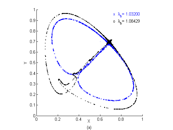
Figure 1: In (a) representation of 2000 points of the chaotic attractor of the Logistic Bimap. In (b) representation of the spectrum of coordinate $x_{t}$. The values of the parameters are $\lambda_{a}=\lambda_{b}=1.032$ in the black curve and $\lambda_{a}=1.032$, $\lambda_{b}=1.084290$ in the blue curve.

In fact, the system is symmetric respective to the diagonal when $\lambda_{a}=\lambda_{b}$. The spectrum of coordinate $x_{t}$ also shows a peak for $w=0.5$, presenting an oscillation of period two that makes it jump over the diagonal axis alternatively between consecutive points in time. Both sub-spaces $x>y$ and $y>x$ are visited with the same frequency and the shape of the attractor is symmetric.

When $\lambda_{b}$ becomes greater than $\lambda_{a}$ the part of the attractor in sub-space $x<y$ becomes wider and the frequency of visits of each sub-space becomes different. This is going to be particularly interesting for our purposes, as the degree of symmetry of the chaotic system is going to be an input variable in the simulations.

3 Chaotic Wealth Distributions

A community of $N=5000$ agents with initial money of $m_{0}=\$1000$ is taken. The Logistic Bimap variables $x_{t}$ and $y_{t}$ in chaotic regime will be used as simulation parameters to obtain trading agents $i$ and $j$. The simulations take a total time of $T=2*N^{2}=50$ millions of transactions.

Different cases are considered, as different values of the chaotic parameters $\lambda_{a}$ and $\lambda_{b}$ are used. In this way the symmetry of the selection of agents is going to vary from total symmetry to the highest value of asymmetry, as it was shown in Fig. 1. Table 1 shows the values of parameters used for the different simulations:

CASE	$1$	$2$	$3$	$4$	$5$	$6$	$7$	$8$
$\lambda_{a}$	$1.032$	$1.032$	$1.032$	$1.032$	$1.032$	$1.032$	$1.032$	$1.032$
$\lambda_{b}$	$1.032$	$1.03781$	$1.04362$	$1.049430$	$1.06105$	$1.07267$	$1.07848$	$1.08429$

Table 1: List of values of $\lambda$ parameter used in the Logistic Bimap for the chaotic simulations.

The resulting money distributions are then obtained as the $\lambda_{b}$ varies from $1.032$ to $1.08429$. In Fig. 2(a), the wealth distribution for the symmetric case is presented. As it can be seen it resembles an exponential distribution. Another interesting point appears in this case. This is the high number of individuals ($1133$ agents) that keep their initial money in Fig. 2(a). The reason is that they don’t exchange money at all. The chaotic numbers used to choose the interacting agents are forcing trades between a deterministic group of them, and hence some trading relations result restricted.

When the passive agents are removed of the model, one can obtain the money distribution of the interacting agents. Fig. 2(b) shows the cumulative distribution function (CDF) obtained for the symmetric case. Here the proba-bility of having a quantity of money bigger or equal to the variable MONEY, is depicted in natural log plot, showing clearly the exponential distribution.

   

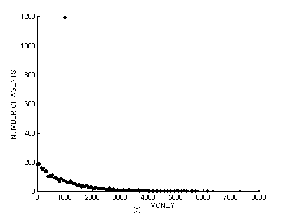
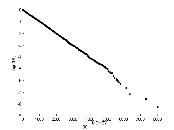
Figure 2: Representations of the final money distribution obtained for chaotic parameters $\lambda_{a}=\lambda_{b}=1.032$. In (a) the distribution with $5000$ agents. A peak can be seen at $\$1000$ with the passive agents. In (b) the cumulative distribution function (CDF) is drawn for the community of real participants ($3867$ agents).

When $\lambda_{b}$ varies from $1.032$ to $1.08429$ it is observed that the number of non-participants decreases. This is because the chaotic map expands (see Fig. 1) and its resulting projections on axis $x$ and $y$ grow in range, taking a greater group of $i$ and $j$ values when equation (2) is computed. Taking these non-participants off the final money distributions, and so their money too, one can obtain the final CDF’s for the different values of $\lambda_{b}$. When these distributions are depicted an interesting progression is shown. As $\lambda_{b}$ increases, these distributions diverge from the exponential shape.

   

Figure 3: Representations of the final CDF’s obtained for chaotic parameters $\lambda_{a}=1.032$ and different values of $\lambda_{b}$. In (a) the distribution up to $\$2000$ dollars is depicted for simulation cases 1,2,3,4 and 5. In (b) these CDF’s are drawn for simulation cases 6,7 and 8.

Fig. 3(a) shows the representation of simulation cases $1$ to $5$ in a natural log plot up to a range of $\$2000$. It can be appreciated that as $\lambda_{b}$ increases, the straight shape obtained for the symmetric case bends progressively, the probability of finding an agent in the state of poorness increases. It also can be seen that for cases 3 and 4, no agent can be found in a middle range of wealth (from $\$1000$ to $\$2000$). This means that the distribution of money is becoming progressively more unequal.

In Fig. 3(b) the CDF’s for simulation cases $6$ to $8$ are depicted from a range of $\$2000$ and in double decimal logarithm plot. Here, a minority of agents reach very high fortunes, what explains, how other majority of agents becomes to the state of poorness. The data seems to follow a straight line arrangement for case $6$, which resembles a Patero distribution. Cases $7$ and $8$ show two straight line arrangements which can also be adjusted to two Pareto distributions of different slopes.

To appreciate these results in a deeper detail, one can consider different economic classes of individuals according to their final status of wealth. The evolution of the population of individuals can be tracked as $\lambda_{b}$ increases. Let us consider three economic classes:“poor class” (with final money from $0$ to $\$500$, “middle class” (from $\$500$ to $\$2000$) and “rich class” (with more than $\$2000$).

CASE	$1$	$2$	$3$	$4$	$5$	$6$	$7$	$8$
Total Money
POOR	$8.80\%$	$9.52\%$	$7.49\%$	$2.89\%$	$1.36\%$	$0.45\%$	$0.18\%$	$0.42\%$
MIDDLE	$51.58\%$	$4.37\%$	$1.71\%$	$0.13\%$	$0.0\%$	$0.0\%$	$0.0\%$	$0.0\%$
RICH	$39.62\%$	$86.11\%$	$90.80\%$	$96.98\%$	$98.64\%$	$99.55\%$	$99.82\%$	$99.58\%$
Total Population
POOR	$39.15\%$	$93.60\%$	$96.71\%$	$98.46\%$	$97.80\%$	$96.92\%$	$96.47\%$	$95.94\%$
MIDDLE	$47.53\%$	$5.94\%$	$2.39\%$	$0.20\%$	$0.0\%$	$0.0\%$	$0.0\%$	$0.0\%$
RICH	$13.32\%$	$0.46\%$	$0.90\%$	$1.35\%$	$2.20\%$	$3.08\%$	$3.53\%$	$4.06\%$

Table 2: Distributions of total traded money and total active agents in different social classes depending on the simulation case.

Table 2 shows how this society is becoming more unequal as $\lambda_{b}$ increases. The middle class even disappears for $\lambda_{b}\geq 1.061050$. The rich gets richer as the asymmetry of the chaotic selection of agents increases and the final amount of money of this class is almost the total money in the system.

What is happening here is, that the asymmetry of the chaotic map is selecting a set of agents preferably as winners for each transaction ($j$ agents). While others, with less chaotic luck become preferably looser ($i$ agents).

Fig. 4 shows, in number of interactions, the times an agent has been a looser (bottom graph) and the difference of winning over losing times (top graph). The $x$ axis shows the ranking of agents ordered by its final money, in a way so that, agent number $0$ is the richest of the community and agent number $5000$ is in the poorest range.

   

Figure 4: Representation of the role of all agents after all the interactions. Agents are arranged in descending order according to their final wealth. The upper graphic shows the total number of wins over looses of an agent. The bottom graphic shows the number of times an agent has been selected as $i$ agent or looser. (a) Simulation case 1, $\lambda_{b}=1.032$. (b) Simulation case 8, $\lambda_{b}=1.084290$.

Fig. 4(a) depicts the symmetric case, where $\lambda_{a}=\lambda_{b}=1.032$. Here, the number of wins and looses is uniformly distributed among the community. There also is a range of agents that don’t interact ($1133$ agents), this can be seen clearly in the figures now. In this case, the chaotic selection of agents show no particular preference and the final distribution becomes the exponential. Similar to traditional simulations with random agents  [2].

Fig. 4(b) shows the same magnitudes for case 8, where $\lambda_{b}=1.084290$ and the asymmetry is maximum. Here it can be seen that there is a group of agents in the range of maximum richness that never loose. The chaotic selection is giving them maximum luck and this makes them richer and richer at every transaction. These are $184$ rich agents (the $4.06\%$ of Table 2). A lower range of agents than in Fig. 4(a) are passive and never interact ($470$ agents). There is no middle class here, and the rest of the community ($4346$ agents) become in state of poorness with a final wealth inferior to $\$500$ and of them, $1874$ agents finish with no money at all.

It is also interesting to see in Fig. 4(b) that in the poor class there are agents that have a positive difference of wins over looses, but amazingly they are poor anyway. Consequently, one can deduce that they are also bad luck guys. They are $j$ agents in most part of their transactions but unfortunately their corresponding trading partners ($i$ agents) are poor too, and they can effectively earn low or no money in these interactions.

4 Conclusions

This work introduces chaotic selection of agents in economic (ideal) gas-like models in a wide range of simulation conditions, where the symmetry of the chaotic map is controlled. This mechanism is able of breaking the pairing symmetry of agents $(i,j)\Leftrightarrow(j,i)$ in trading markets. The distributions of money obtained this way, exhibit a transition from Gibbs to Pareto distributions, as the pairing symmetry is progressively broken.

More over, it illustrates how a small group of people can be chaotically destined to be very rich, while the bulk of the population ends up in state of poverty. This may resemble some realistic conditions, showing how some individuals can accumulate big fortunes in trading markets, as a natural consequence of the intrinsic asymmetric conditions of real economy.

Acknowledgements The authors acknowledge some financial support by Spanish grant DGICYT-FIS200612781-C02-01.

References

- [1] R. Mantegna, H.E. Stanley. An Introduction to Econphysics: Correlations and Complexity in Finance. Cambridge University Press, ISBN 0521620082, 2000.
- [2] V.M. Yakovenko. Econophysics, Statistical Mechanics Approach to. Encyclopedia of Complexity and System Science, ISBN 9780387758886, Springer, 2009. (Available at arXiv:0709.3662v4).
- [3] A.A. Dragulescu, V.M. Yakovenko. Statistical mechanics of money. The European Physical Journal B, 17:723-729, 2000.(Available at arXiv:cond-mat/0001432).
- [4] A. Chakraborti, B.K. Chakrabarti. Statistical mechanics of money: how saving propensity affects its distribution. The European Physical Journal B, 17:167-170, 2000.
- [5] J.P. Bouchaud, M. Mézard. Wealth condensation in a simple model economy. Physica A, 282: 536-545, 2000.
- [6] B.K. Chakrabarti, S. Marjit. Self-organization in Game of Life and Economics. Indian Journal Physics B, 69:681-698, 1995.
- [7] A.A. Dragulescu, V.M. Yakovenko. Exponential and power-law probability dstributions of wealth as income in the United Kindom and the United States. Physica A, 299:213-221, 2001. (Available at arXiv:cond-mat/0103544v2).
- [8] O.S. Klass, O. Biham, M. Levy, O. Malcai, S. Solomon. The Forbes 400 and the Pareto wealth distribution. Economics Letters, 90:290-295, 2006.
- [9] C. Pellicer-Lostao, R. López-Ruiz. Economic Models with Chaotic Money Exchange. Proceedings of the ICCS 2009, Lectures Notes of Computer Sciences, Part I, 5544:43-52, 2009. (Available at arXiv:0901.1038).
- [10] R. Lopez-Ruiz. Transiton to Chaos in Different Families of Two-Dimensional Mappings. Tesina, Dep. of Physics, University of Navarra, 1991 ; R. Lopez-Ruiz, C. Pérez-Garcia. Dynamics Maps with a Global Multiplicative Coupling. Chaos, Solitons and Fractals, 1:511-528, 1991.
- [11] C. Pellicer-Lostao, R. López-Ruiz. Orbit Diagram of Two Coupled Logistic Maps Wolfram Demonstrations Project. URL: http://demonstrations.wolfram.com/OrbitDiagramOfTwoCoupledLogisticMaps.