New insight on pseudospin doublets in nuclei

Abstract

The relevance of the pseudospin symmetry in nuclei is considered. New insight is obtained from looking at the continuous transition from a model satisfying the spin symmetry to another one satisfying the pseudospin symmetry. This study suggests that there are models allowing no missing single-particle states in this transition, contrary to what is usually advocated. It rather points out to an association of pseudospin partners different from the one usually assumed, together with a strong violation of the corresponding symmetry. A comparison with results obtained from some relativistic approaches is made.

PACS: 21.60.Cs Shell model, 24.80.+y Nuclear tests of fundamental interactions and symmetries, 24.10.Jv relativistic models, 21.10.Pc Single-particle levels and strength functions

Keywords: Pseudospin doublets; Atomic nuclei

1 Introduction

The concept of pseudospin symmetry (PSS) in the description of single-particle nuclear levels has been introduced 40 years ago [1, 2]. It was motivated by the observation that levels within the same major shell such as $2s_{1/2}$ and $1d_{3/2}$ ($N=2$), $2p_{3/2}$ and $1f_{5/2}$ ($N=3$), etc, are rather close to each other and, in any case, closer than usual spin-orbit partners. Thus, the pseudospin symmetry could be more accurately satisfied than the spin symmetry (SS). Approximate pseudospin symmetry has been also found and analyzed in deformed nuclei [3]-[5] before a general explanation were suggested and lengthily accepted.

Some theoretical explanation supporting the existence of pseudospin doublets was given by Ginocchio [6], within the phenomenological relativistic framework originally proposed by Walecka for nuclear matter [7] and used later on for studying properties of finite nuclei [8, 9]. Looking at the small components of the Dirac spinors [10], he noticed that the equation allowing one to determine them leads to degenerate pseudospin (PS) doublets in the limit where the sum of the scalar ($\Sigma_{S}$) and vector ($\Sigma_{0}$) components of the nucleon self-energies vanishes. In this limit, the radial parts of the small components are identical. This result suggested him to propose that the approximate pseudospin symmetry is due to the fact that the sum of the scalar and vector self-energies, $\Sigma_{S}$ and $\Sigma_{0}$, cancels for a large part [11]-[15]. The attractive explanation of the pseudospin symmetry has motivated a considerable number of studies by other authors both to extend its result [16]-[24] and to get a better understanding of its limitations [25]-[39]. Among these last ones, it was noticed that the quasi cancellation of the self-energies in the sum $\Sigma_{S}+\Sigma_{0}$ was associated with an energy denominator which, actually, does cancel at the nuclear surface [25]-[31], [34]. This indicates that some care is required in concluding from the cancellation of the $\Sigma_{S}$ and $\Sigma_{0}$ potentials alone [32]. Thus, the expected similarity of the radial part of the small components of the Dirac spinors was not strongly supported by the detailed analysis of various solutions [28, 31]. It even turned out that the similarity of the radial part of the large components for spin-orbit partners was better satisfied while the conditions for the energy levels required by the symmetry in this case are apparently worse [28, 31]. Last, but not least, the pseudospin symmetry supposes the existence of single-particle states that are not observed [14], i.e. the PS partners of the so-called intruder states (states with $n=1$ and $j=l+1$). For clarifying some of the above points, a model where the above mentioned energy denominator does not cancel would be useful. In this case, however, any realistic nuclear model would not admit bound states.

In this work, we mainly concentrate on the possible missing states. For our purpose, we first work in the non-relativistic case and consider two interactions that evidence the spin and pseudospin symmetry. For simplicity, we assume that they are related to each other by a unitary transformation that commutes with the kinetic-energy operator. To study specifically the missing-state problem, we also introduce an interaction that is a superposition of the two above ones with relative weights, $1-x$ and $x$. By varying the $x$ parameter from $0$ to $1$, one should see how energy levels in the spin-symmetry case are related (or unrelated) to those in the pseudospin-symmetry one and vice versa. Some extension to a relativistic approach is made with the idea of an application to clarifying Chen et al. results [22], which evidence a spectrum very similar to ours in the nonrelativistic approach. Tentatively, we also considered the case of finite potentials instead of harmonic-oscillator-type ones used in the above work.

The plan of the paper is as followed. The second section is devoted to the general aspects of the non-relativistic interaction we are using for our study. Results for spectra obtained from two different interaction models are presented in the third section together with some discussion. Complementary information from examining wave functions is given in the fourth section. The fifth section is devoted to a comparison with results from relativistic approaches. Conclusions are given in the sixth section. Two appendices contain some technical details.

2 Interaction model

The interactions with spin and pseudospin symmetry we start with may be written as:

$$V_{0}=V_{0}(r)\,,$$

$$\tilde{V}_{1}=\vec{\sigma}\!\cdot\!\hat{p}\,V_{1}(r)\,\vec{\sigma}\!\cdot\!\hat{p}\,,$$ (1)

where $V_{0}(r)$ and $V_{1}(r)$ are spin independent and only depend on the $r$ variable (local potentials). The operator $\vec{\sigma}\!\cdot\!\hat{p}$ appearing in $\tilde{V}_{1}$ is an unitary one. It changes the states corresponding to the pseudospin-symmetry space (represented with the symbol $\tilde{}\,$) to those corresponding to the spin-symmetry space [40]. In this operation, the total angular momentum, $j$, is preserved while the orbital angular momentum is modified by one unit, implying a change of parity. Moreover, the operator makes the interaction $\tilde{V}_{1}$ non local. The corresponding Hamiltonian may therefore be written as:

$$\tilde{H}_{1}=\frac{p^{2}}{2M}+\tilde{V}_{1}=\vec{\sigma}\!\cdot\!\hat{p}\,\Big{(}\frac{p^{2}}{2M}+V_{1}(r)\Big{)}\,\vec{\sigma}\!\cdot\!\hat{p}\,,$$ (2)

indicating that the spectra corresponding to the interactions $\vec{\sigma}\!\cdot\!\hat{p}\,V_{1}(r)\,\vec{\sigma}\!\cdot\!\hat{p}$ and $V_{1}(r)$ will be the same, apart from the spin-orbital angular momentum assignments of course. Wave functions for the Hamiltonian $\tilde{H}_{1}$ can be obtained from those for the Hamiltonian $H_{1}=\frac{p^{2}}{2M}+V_{1}(r)$ by applying to these ones the operator $\vec{\sigma}\cdot\hat{p}$. Apart from the angular-momentum factor, the solutions of $H_{1}$ for spin-orbit partners are the same in both configuration and momentum spaces. As the operator $\vec{\sigma}\!\cdot\!\hat{p}$ is local in momentum space, this equality will turn into an equality for momentum-space solutions of $\tilde{H}_{1}$ corresponding to pseudospin partners.

The total interaction that is useful for our purpose of looking at the transition of the spin-symmetry case to the pseudospin-symmetry one may be written as:

$$V(r) = (1-x)\,V_{0}+x\,\tilde{V}_{1}$$ (3)

$$= (1-x)\,V_{0}(r)+x\,\vec{\sigma}\!\cdot\!\hat{p}\,V_{1}(r)\,\vec{\sigma}\!\cdot\!\hat{p}\,,$$

where $x$ is supposed to vary from $0$ to $1$. Actually, as the interaction $\tilde{V}_{1}$ is spin dependent, we can recover a part of the usual spin-orbit splitting by taking slightly negative values of $x$.

	spin symmetry		pseudospin symmetry
	$2p_{1/2},\;2p_{3/2},\;1f_{5/2},\;1f_{7/2}$	$\leftrightarrow$	$2\tilde{s}_{1/2},\;2\tilde{d}_{3/2},\;\;\;1\tilde{d}_{5/2},\;1\tilde{g}_{7/2}$
	$2s_{1/2},\;1d_{3/2},\;1d_{5/2}$	$\leftrightarrow$	$2\tilde{p}_{1/2},\;\;\;1\tilde{p}_{3/2},\;1\tilde{f}_{5/2}$
	$1p_{1/2},\;1p_{3/2}$	$\leftrightarrow$	$1\tilde{s}_{1/2},\;1\tilde{d}_{3/2}$
	$1s_{1/2}$	$\leftrightarrow$	$1\tilde{p}_{1/2}$

Table 1: Representation of spectra in the spin-symmetry and pseudospin-symmetry limit (l.h.s. and r.h.s. respectively): states on the left in each row correspond to standard major shells. For the interaction assumption $V_{1}(r)=V_{0}(r)$ considered in this work, states on the r.h.s. in a given row have the same energy as those on the l.h.s. in the same row and the same total angular momentum (but a different parity). We anticipated that the quantum number $n$ is preserved in making this correspondence.

As mentioned in the introduction, we consider the particular case where $V_{1}(r)=V_{0}(r)$. This does not diminish the relevance of results to be obtained here, making them more striking instead. Without performing any calculation, one can see that the states for the spin and pseudospin-symmetry cases, shown respectively in the l.h.s. and r.h.s. of Table 1, are in a one-to-one correspondence. The $n$ quantum number represents the order of the states and, apart from a possible conventional shift by one unit, it is not, necessarily, identical to the node number of the radial wave function. This relationship, which is often assumed implicitly in the literature, is specific of a local potential. The question of interest is whether there is a global continuity between states on the l.h.s. of the table and those on the r.h.s. when the interaction varies from the spin-symmetry limit ($x=0$) to the pseudospin-symmetry one ($x=1$). It is reminded that the current understanding of the pseudospin symmetry supposes that the pseudospin partners of the states on the very right in each row of the left part of Table 1 are absent, due to specific conditions of realistic nuclear potentials [14]. The argument relies on a mathematical analysis of the nodes of wave functions. The authors do not examine in what measure this absence could have a relation with the differences between realistic models and those satisfying exact PSS. As we shall see in this work, as one approaches the PSS limit, a new type of nodes could appear, which may affect their conclusion.

It remains to specify the choice of the potential $V_{0}(r)(=V_{1}(r))$. We consider two choices inspired by the harmonic-oscillator and the Woods-Saxon potentials. The comparison of results for these two models evidences a little but important detail that could be relevant for the interpretation of pseudospin doublets. The absence of singular behavior for these potentials lets one to expect a continuous transition between states on the l.h.s. and r.h.s. of Table 1.

3 Results and discussion for the spectra

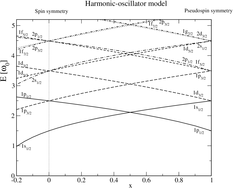
Figure 1: Single-particle spectrum evidencing the spin- and pseudospin-symmetry cases and the continuous transition between them. The interaction is based on a harmonic-oscillator one: $V=\frac{1}{2}M\omega_{0}^{2}\;\Big{(}(1\!-\!x)\;r^{2}+x\;\vec{\sigma}\!\cdot\!\hat{p}\;r^{2}\;\vec{\sigma}\!\cdot\!\hat{p}\Big{)}$. The observed order of the spin-orbit partners is recovered for negative values of $x$. The figure includes on the l.h.s. two “standard pseudospin doublets”, $1d_{3/2}$ and $2s_{1/2}$ on the one hand, $1f_{5/2}$ and $2p_{3/2}$ on the other hand.

We, successively, present in this section level spectra for the harmonic-oscillator (HO) and the Woods-Saxon (WS) models. Parameters are those appropriate to the description of a nucleus such as ${}^{40}Ca$. This is followed by some comments about the spectra.

3.1 Harmonic-oscillator model

For the potential $V(r)$ inspired from the harmonic-oscillator form, the two terms $V_{0}(r)$ and $V_{1}(r)$ entering its definition assume the standard form:

$$V_{0}(r)=V_{1}(r)=\frac{1}{2}M\omega_{0}^{2}\,r^{2}\,.$$ (4)

As results for the energy levels only depend on the parameter $\omega_{0}$, it is sufficient to present them in units of this parameter. They are shown in Fig. 1 for $x$ varying from -0.2 to 1. Actually, calculations were done with a Gaussian potential deep enough to be approximated by the HO potential. The reason is that this is more convenient for our study, which is made in the momentum space due to the non-locality of the interaction model we are using when $x\neq 0$. Moreover, the Fourier transform of the Gaussian potential can easily be performed. As can be observed from the figure, there is almost no departure with the results of the harmonic-oscillator model when a comparison is possible (at $x=0$). While the spectra can be essentially given in terms of $\omega_{0}$, the value taken by this parameter is nevertheless relevant in obtaining wave functions that could be compared to those of the WS model. We use $\omega_{0}=7$ MeV so that the spectra of the HO and WS models roughly overlap.

Examination of the spectrum around $x=-0.2$ shows it a priori contains the two standard pseudospin doublets, $1d_{3/2},\;2s_{1/2}$ and $1f_{5/2},\;2p_{3/2}$, though the corresponding states are slightly apart in each case. The comparison with the spectrum at $x=1$, which evidences an exact pseudospin symmetry, suggests a different pattern however. The states $1d_{3/2}$ and $2s_{1/2}$ (or $1f_{5/2}$ and $2p_{3/2}$) tend to separate in this limit while the states $1d_{3/2}$ and $1s_{1/2}$ (or $1f_{5/2}$ and $1p_{3/2}$) get closer, supporting that these ones should be associated in the same pseudospin doublet. We notice that the assignment of the $n$ quantum number to the different states is made by continuity with results at $x=0$. In this case, where the potential is local, there is a one-to-one correspondence between this number and the number of nodes in the radial wave function. This correspondence is lost as soon as the interaction is partly non-local. Examination of radial wave functions like the $1s_{1/2}$ for $x=1$ thus evidences a node. This one occurs however in the tail of the wave function, at a distance where the contribution to the normalization is almost saturated (within a few percent’s). It differs from standard nodes that allow one to determine contributions to the normalization from smaller and larger $r$ of comparable sizes. Only these ones could have some relation to the quantum number $n$. We also notice that the pseudospin-symmetry spectrum obtained for $x=1$ shows the same degeneracy pattern as the one obtained by Chen et al. in a relativistic approach with a harmonic-oscillator-type interaction [22]. Whether there is a relationship between the two cases will be discussed in Sect. 5.

3.2 Woods-Saxon model

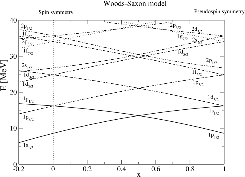
Figure 2: Same as in Fig. 1, but for the Woods-Saxon model

For the potential $V(r)$ inspired from the Woods-Saxon form, the two terms $V_{0}(r)$ and $V_{1}(r)$ entering its definition assume the standard form:

$$V_{0}(r)=V_{1}(r)=-\frac{V_{0}}{1+{\rm exp}((r-r_{0})/a))}\,.$$ (5)

      

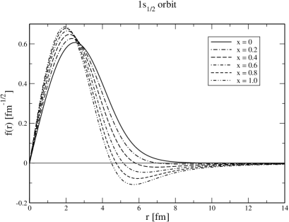
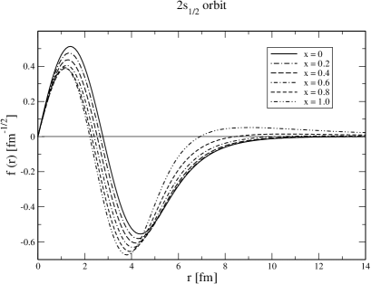
Figure 3: Appearance of an extra node when going from the spin- to the pseudospin-symmetry limit for orbits $1s_{1/2}$ and $2s_{1/2}$ (left and right panels respectively) with the Woods-Saxon model. It is noticed that the extra node appears in the tail of the wave function and cannot be confused with the usual nodes that appear at smaller distances, as the comparison of the two panels can show. The wave functions are normalized as $\int dr\,f^{2}(r)=1$.

      

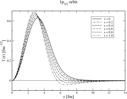
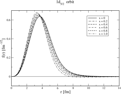
Figure 4: Same as for Fig. 3 but for orbits $1p_{3/2}$ and $1d_{5/2}$ (left and right panels respectively).

For numerical calculations, we use $V_{0}=40$ MeV, $r_{0}=5$ fm, $a=0.65$ fm. Results for the spectrum are shown in Fig. 2. Examination of this figure confirms most of the features observed for the HO model. The energies of the two members of the pseudospin symmetry doublets, $1d_{3/2},\;2s_{1/2}$ and $1f_{5/2},\;2p_{3/2}$, are closer to each other however. As for the HO model, the quantum number, $n$, has been assigned by continuity with the spin-symmetry case. This quantum number is not necessarily related to the number of nodes as often assumed implicitly. Thus, orbits with $j=l+\frac{1}{2}$ tend to get an extra node when going gradually from the spin- to the pseudospin-symmetry limit while orbits with $j=l-\frac{1}{2}$ don’t. The extra node occurs at the limit or outside the range of the potential $V_{1}(r)$. This is illustrated in Fig. 3 for the orbits $1s_{1/2}$ and $2s_{1/2}$ and in Fig. 4 for the orbits $1p_{3/2}$ and $1d_{5/2}$. The contribution to the norm beyond the extra node amounts to 3% in the largest case and tend to decrease either with going to the spin-symmetry limit or with increasing the orbital angular momentum. In comparison, the contribution to the norm for a usual node amounts to several 10% (see the two panels of Fig. 3 for a $s_{1/2}$ orbit).

3.3 Comments

Examination of the spectra for two interaction models shows that there is essentially a one-to-one global correspondence between states with the spin symmetry ($x=0$) and those with the pseudospin symmetry ($x=1$). There is no indication for missing pseudospin partners as often advocated. Instead, all states are there but in a different order. The order for the pseudospin-symmetry states may be a surprise but this is a consequence of the non locality of the corresponding interaction used here.

The interaction model we used does not contain explicit spin-orbit interaction but it is found that the nonlocal term proportional to $V_{1}$ provides a similar effect which, for $x=-0.2$, has the appropriate size. This is not unexpected as there is some similarity of this term with the one that produces the effect in relativistic mean-field approaches where it is proportional to $\vec{\sigma}\!\cdot\!\vec{p}\;V_{1}(r)\,\vec{\sigma}\!\cdot\!\vec{p}$. We also notice that the actual description of nuclei ($x=-0.2$) is closer to the PS limit ($x=0$) than to the PSS limit ($x=1.0$) and, moreover, requires an opposite-sign value of $x$.

Our last comment is motivated by the comparison of the two models concerning the standard pseudospin doublets. While results for the WS model at $x=-0.2$ supports such doublets, this is not the case for the HO model. It is known from the Nilsson model that a term proportional to $-\kappa\;\mu\;\vec{l}\,^{2}$ could be necessary to improve the single-particle spectrum, lowering, for instance, the energy of the $1d_{3/2},\;1d_{5/2}$ states with respect to the $2s_{1/2}$ one. This feature shows that the form of the potential is important in getting the standard pseudospin doublets. This contrasts with the explanation of these doublets in the relativistic mean-field approach [6], which assumes that the approximate PS symmetry observed in this approach is, essentially, a direct consequence of the small size of $\Sigma_{S}+\Sigma_{0}$ (in comparison with the magnitude of $\Sigma_{S}-\Sigma_{0}$ [12]), independently of its form.

4 Results and discussion for the wave functions

In discussing pseudospin doublets, examination of the corresponding wave functions is thought to provide an important information on the relevance of the possible underlying symmetry. In this section, we present results based on wave functions for the standard pseudospin-symmetry partners as well as those resulting from our interpretation of the doublets. This is done in both momentum and configuration space, for the two interaction models we considered and for the two doublets that their spectra shown in Figs. 1 and 2 exhibit.

     

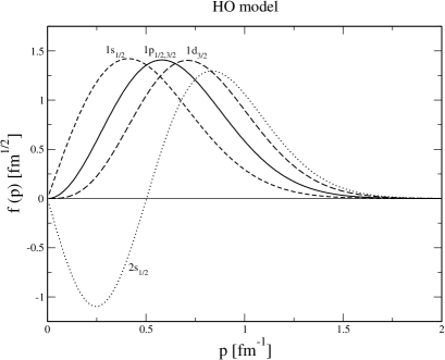
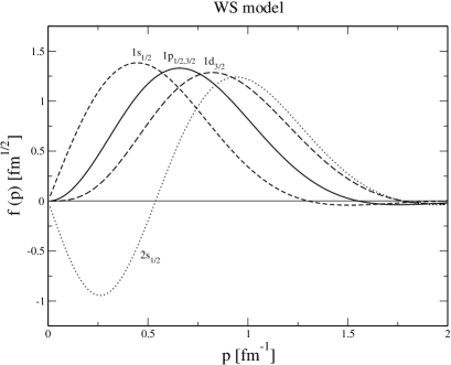
Figure 5: Comparison of momentum-space wave functions, $f(p)$, for the lowest pseudospin doublet with the HO and WS models (left and right panels respectively): small- and large-dash lines for the states $1s_{1/2},\;1d_{3/2}$, continuous line for the limit expected in the pseudospin-symmetry limit and dotted line for the $2s_{1/2}$ state. All wave functions shown in the figure are calculated at $x=0$.

     

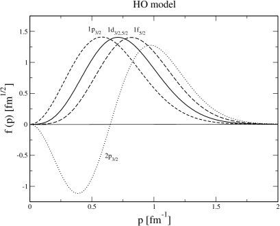
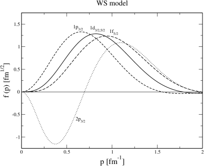
Figure 6: Comparison of momentum-space wave functions, $f(p)$, for the second lowest pseudospin doublet with the HO and WS models (left and right panels respectively): small- and large-dash lines for the states $1p_{3/2},\;1f_{5/2}$, continuous line for the curve expected in the pseudospin-symmetry limit and dotted line for the $2p_{3/2}$ state. All wave functions shown in the figure are calculated at $x=0$.

4.1 Results in momentum space

The transformation of the usual spin space to the pseudospin one, given by the operator $\vec{\sigma}\cdot\hat{p}$, is local in the momentum space, where its effect can therefore be more easily calculated. Thus, the spin-orbital angular momentum part of wave functions for the states $d_{3/2},\;s_{1/2}$ (or $f_{5/2},\;p_{3/2}$) transform into that for the states $\tilde{p}_{3/2},\;\tilde{p}_{1/2}$ (or $\tilde{d}_{5/2},\;\tilde{d}_{3/2}$), leaving unaffected the dependence on the modulus of $\vec{p}$, which we denote $f(p)$. In the pseudospin-symmetry limit, these functions for the states $\tilde{p}_{3/2},\;\tilde{p}_{1/2}$ (or $\tilde{d}_{5/2},\;\tilde{d}_{3/2}$) are the same. Hence, in this limit, the functions $f(p)$ for the states $d_{3/2},\;s_{1/2}$ (or $f_{5/2},\;p_{3/2}$) should be equal. Moreover, the functions for the states $\tilde{p}_{3/2},\;\tilde{p}_{1/2}$ (or $\tilde{d}_{5/2},\;\tilde{d}_{3/2}$) can be calculated in this limit. For our interaction model, it is simply given by the functions for the states $p_{3/2},\;p_{1/2}$ (or $d_{5/2},\;d_{3/2}$) in the spin-symmetry limit. We thus get relations like the following ones:

$$f_{1d_{3/2}}(p)=f_{1s_{1/2}}(p)=f_{1p_{1/2,3/2}}(p)\,,$$

$$f_{1f_{5/2}}(p)=f_{1p_{3/2}}(p)=f_{1d_{3/2,5/2}}(p)\,.$$ (6)

One can therefore compare the $f(p)$ functions for the pseudospin doublet, according to our interpretation, $1d_{3/2},\;1s_{1/2}$ (or $1f_{5/2},\;1p_{3/2}$), for the spin doublet $1p_{3/2},\;1p_{1/2}$ (or $1d_{5/2},\;1d_{3/2}$), and for the standard pseudospin doublet $1d_{3/2},\;2s_{1/2}$ (or $1f_{5/2},\;2p_{3/2}$) (where we substituted the state $2s_{1/2}$ (or $2p_{3/2}$) for the state $1s_{1/2}$ (or $1p_{3/2}$)). For the purpose of the comparison, the functions for the pseudospin doublet $d_{3/2},\;s_{1/2}$ (or $f_{5/2},\;p_{3/2}$) are calculated at $x=0$. They fulfill the following normalization condition:

$$\int dp\;f^{2}(p)=1\,.$$ (7)

The corresponding results are shown in Figs. 5 and 6 for the lowest and next to the lowest pseudospin doublet respectively. In each case, results for the two interaction models are shown.

A quick look at the results with the two interaction models, as well as for the two pseudospin doublets, according to our definition, does not evidence much qualitative difference in the range which mainly contributes to the normalization. As the pseudospin symmetry is not fulfilled at the point $x=0$ where the functions $p_{3/2},\;p_{1/2}$ (or $d_{5/2},\;d_{3/2}$) are calculated, one expects that the various curves shown in the figures evidence some discrepancy. With this respect, these discrepancies are not small. At low $p$, they essentially reflect the $p^{l+1}$ behavior expected for a local interaction model. At higher $p$, they rather reflect the average momentum of the state, which increases with its energy as measured from the bottom of the potential well. It is nevertheless seen that functions $f(p)$ for the pseudospin doublets, as considered here, have a unique sign in the range which mainly contributes to the norm. Moreover, they share this feature with the function expected in the pseudospin symmetry limit. Instead, the functions for the standard pseudospin doublets evidence a different structure in the same range. One of the function has a given sign while the other one (with a different $n$ number) evidences a change in sign. It thus turns out that our assignment for pseudospin doublets is more in agreement with the pseudospin-symmetry expectation than the standard assignment.

4.2 Results in configuration space

     

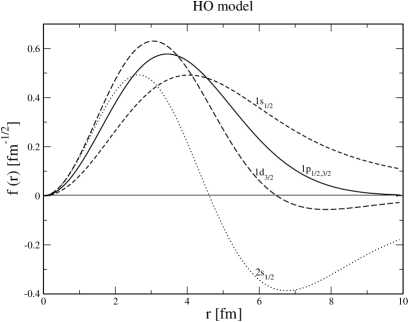
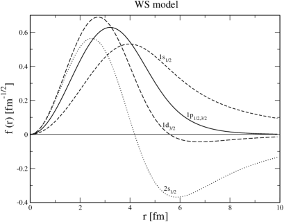
Figure 7: Comparison of configuration-space wave functions for the lowest pseudospin doublet with the HO and WS models (left and right panels respectively). See caption of Fig. 5 for the definition of the different curves.

     

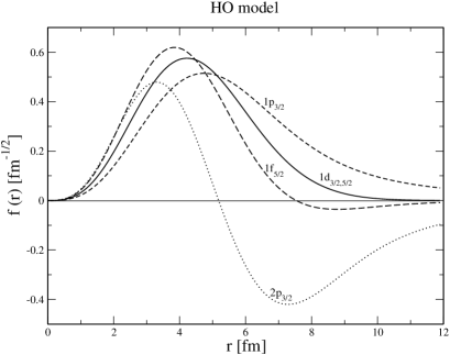
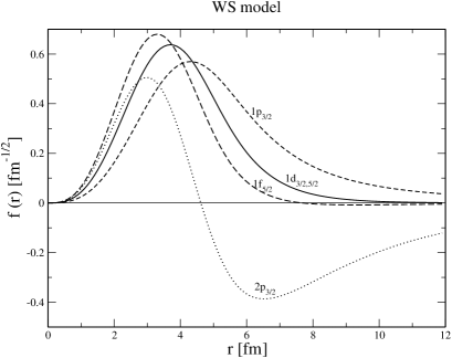
Figure 8: Comparison of configuration-space wave functions for the second lowest pseudospin doublet with the HO and WS models (left and right panels respectively). See caption of Fig. 6 for the definition of the different curves.

While the direct comparison of wave functions in momentum space makes sense, it does not in configuration space where wave functions imply an integral over $p$ of momentum wave functions together with spherical Bessel functions of different $l$. A possible comparison could involve the integral of the different momentum wave functions with the same spherical Bessel function $j_{1}(pr)$ for the lowest pseudospin doublet (or $j_{2}(pr)$ for the second one). We defined these quantities as:

$$f(r)=\sqrt{\frac{2}{\pi}}\;r\int dp\;f(p)\;j_{1}(pr)\;({\rm or}\;j_{2}(pr))\,,$$ (8)

which, using Eq. (7), are found to verify the normalization condition:

$$\int dr\;f^{2}(r)=1\,.$$ (9)

Interestingly, the quantities $f(r)$ together with the associated angular momentum structure corresponding to the states $p_{3/2},\;p_{1/2}$ (or $d_{5/2},\;d_{3/2}$), show some similarity with the small components in the Dirac mean-field phenomenology. It is reminded that the examination of the equation allowing one to determine these components provided some justification for the existence of pseudospin doublets [6, 11]. Taking into account Eq. (6), the functions $f(r)$ are expected to verify the following relation in the pseudospin-symmetry limit:

$$f_{1d_{3/2}}(r)=f_{1s_{1/2}}(r)=f_{1p_{1/2,3/2}}(r)\,,$$

$$f_{1f_{5/2}}(r)=f_{1p_{3/2}}(r)=f_{1d_{3/2,5/2}}(r)\,.$$ (10)

Results showing the $f(r)$ functions are presented in Figs. 7 and 8, in full correspondence with those shown in Figs. 5 and 6 for momentum space. Qualitatively, the different curves evidence a similar pattern. There is not much sensitivity to the interaction model and the slight sensitivity to the pseudospin doublet can be mainly ascribed to the corresponding binding, the results for the less bound system tending to extend to larger radial distances.

In each panel, curves corresponding to the pseudospin assignment made here have the same sign within the largest range of their contribution to the normalization given by Eq. (9). They evidence some spreading but fall slightly apart on one side and on the other side of the expected result in the pseudospin-symmetry limit. The curves corresponding to the standard pseudospin assignment evidence a striking difference. One of them changes sign within the range of its main contribution to the normalization. Thus, these results show that, like in momentum space, if one considers only the similarity of the $f(r)$ functions of the PS partners, it is more natural to consider the states $1d_{3/2},\;1s_{1/2}$ (or $1f_{5/2},\;1p_{3/2}$), as a pseudospin doublet rather than the states $1d_{3/2},\;2s_{1/2}$ (or $1f_{5/2},\;2p_{3/2}$). The argument will get further strength if we notice that the above spreading represents for a large part a difference in the binding energy or in the momentum distribution of the wave functions. It is found that Eq. (10) is much better fulfilled than what Figs. 7 and 8 suggest if we require that the average square momentum be the same, as expected in the pseudospin-symmetry limit. This can be checked by using scaled wave functions.

5 Relation with results from a relativistic approach

Since the PS symmetry has been considered in the last decade as a symmetry with deep roots in the relativistic theory of atomic nuclei [6], arises the question of whether the above results can be cast into this approach, which can be described by the following equations:

$$\vec{\sigma}\!\cdot\!\vec{p}\;\;\psi_{<}(\vec{r})-(E-M-V(r))\;\psi_{>}(\vec{r})=0,$$

$$\vec{\sigma}\!\cdot\!\vec{p}\;\;\psi_{>}(\vec{r})-(E+M-\Delta(r))\;\psi_{<}(\vec{r})=0.$$ (11)

where $\psi_{>}(\vec{r})$ and $\psi_{<}(\vec{r})$ represent, respectively, the usual large and small component of the Dirac spinor. Various models are considered in the following.

5.1 Model inspired from the non-relativistic one

Generally, the potentials $V(r)$ and $\Delta(r)$ are taken as the sum and the difference of the scalar and vector potentials, $V(r)=V_{v}(r)+V_{s}(r)$ and $\Delta(r)=V_{v}(r)-V_{s}(r)$, but , formally, nothing prevents one to take $V(r)$ as given by Eq. (3) and $\Delta(r)$ as a constant. This model has not much to do with the usual relativistic mean-field phenomenology but it can be easily studied. Actually, it does not add relevant information to the non-relativistic model studied in the previous section. Very similar results are obtained for the spectrum as well as for the wave function as far as the large component is concerned.

5.2 Model inspired from the Chen et al. one

A more interesting comparison involves the model considered by Chen et al. [22, 23]. Apart from the energy scale, the pseudospin-symmetry spectrum shown in Fig. 1 evidences a striking similarity with theirs. There could be also some similarity with results obtained by Lisboa et al. [36], which are essentially the same as those obtained by Chen et al., but the authors modified the assignment of the quantum number $n$ to make it identical to the number of nodes of the radial wave functions. The authors compare the results in the cases of the two symmetry limits, arguing about missing and intruder states. The question therefore arises whether there is a continuity between the two limits, as observed in the non-relativistic case discussed in previous sections. Such a study could also help in clarifying the assignment of the $n$ quantum number.

In order to study the relationship between the two symmetry cases, one has to determine the two potentials, $V(r)$ and $\Delta(r)$, that enter the following standard equations for the large and small components, $G(r)$ and $F(r)$:

$$\Bigg{[}\!-\frac{d^{2}}{dr^{2}}\!+\!\frac{l(l\!+\!1)}{r^{2}}-(E\!+\!M\!-\!\Delta(r))\,(E\!-\!M\!-\!V(r))\Bigg{]}\,G(r)-\frac{\frac{d\Delta(r)}{dr}(\frac{d}{dr}\!+\!\frac{\kappa}{r},\,G(r))}{E\!+\!M\!-\!\Delta(r)}=0\,,$$ (12)

$$\Bigg{[}\!-\frac{d^{2}}{dr^{2}}\!+\!\frac{\tilde{l}(\tilde{l}\!+\!1)}{r^{2}}-(E\!+\!M\!-\!\Delta(r))\,(E\!-\!M\!-\!V(r))\Bigg{]}\,F(r)-\frac{\frac{dV(r)}{dr}(\frac{d}{dr}\!-\!\frac{\kappa}{r},\,F(r))}{E\!-\!M\!-\!V(r)}=0\,,$$ (13)

where the notation such as $(\frac{d}{dr}\!+\!\frac{\kappa}{r},\,G(r))$ stands for $(G^{\prime}(r)\!+\!\frac{\kappa}{r}\,G(r))$. In the cases of spin- and pseudospin-symmetry limits, the potentials $V(r)$ and $\Delta(r)$ should be respectively given by:

$$V(r)=V_{0}(r)=\frac{1}{2}\omega^{2}Mr^{2}, \hskip 45.52458pt\Delta(r)=0\,,$$ (14)

$$V(r)=0, \hskip 28.45274pt\Delta(r)=\Delta_{0}(r)=\frac{1}{2}\omega^{2}Mr^{2}\,.$$

A first guess to determine the transition potential would consist in multiplying $V_{0}(r)$ and $\Delta_{0}(r)$ by the factors $1-x$ and $x$, and allow $x$ to vary between 0 and 1. It can be however shown that solutions of Eqs. (12, 13) have then an oscillatory behavior at large $r$, which complicates their determination and could obscure conclusions. As we are interested in finding at least one way to ensure a continuous transition between the two symmetry limits, we proceed differently. Instead of fixing a priori the transition potential, we determine this potential from minimal consistency conditions. To illustrate the method we adopted, we consider here with some detail the case $n=1$ and $l=\tilde{l}+1$.

First, as the above mentioned oscillatory character of solutions is due to the appearance of an attractive $r^{4}$ term in the product $(M\!+\!E\!-\!\Delta(r))\,(M\!-\!E\!+\!V(r))$, we skip this term so that the remaining part behaves as an ordinary harmonic-oscillator potential. This product thus read:

$$(E\!+\!M\!-\!\Delta(r))(E\!-\!M\!-\!V(r))=E^{2}\!-\!M^{2}-\frac{M\omega^{2}r^{2}}{2}\Big{(}(1\!-\!x)(E\!+\!M)+x(E\!-\!M)\Big{)}\,.$$ (15)

It allows one to determine $V(r)$ once $\Delta(r)$ has been determined from other sources. Second, the examination of the last term in Eq. (12) in the pseudospin-symmetry limit ($V(r)=0$) shows that the singular behavior due to its denominator is exactly cancelled by the action on $G(r)$ of the operator, $\frac{d}{dr}\!+\!\frac{\kappa}{r}$, at the numerator. The equation can then be solved analytically, allowing one to recover the solution which is known in any case. It is not difficult to see that the procedure can be extended to any $x$ in the simplest case of orbits with $n=1$ and $l=\tilde{l}+1$ (states $1p_{1/2},\;1d_{3/2},\;1f_{5/2},\;1g_{7/2},\cdots$). The solution assumes the form:

$$G(r)\propto r^{(l+1)}\,{\rm exp}(-\alpha^{2}\,r^{2}/2)\,,$$ (16)

while the last term in Eq. (12) can be written as:

$$-\frac{\frac{d\Delta(r)}{dr}(\frac{d}{dr}\!+\!\frac{\kappa}{r},\,G(r))}{E\!+\!M\!-\!\Delta(r)}=-\frac{\frac{d\Delta(r)}{dr}\;(2l\!+\!1\!-\!\alpha^{2}\,r^{2})}{(E\!+\!M\!-\!\Delta(r))\;r}\,G(r)=-x\,\frac{(2l\!+\!1)\,\omega^{2}M}{E\!+\!M}\,G(r)\,.$$ (17)

By inserting the above expression in Eq. (12), one gets the following relations to be fulfilled:

$$\alpha^{2}-\omega\,\sqrt{\frac{M}{2}\Big{(}(1\!-\!x)(E\!+\!M)+x(E\!-\!M)\Big{)}}=0\,,$$ (18)

$$E^{2}\!-\!M^{2}-\omega\,(2l\!+\!3)\;\sqrt{\frac{M}{2}\Big{(}(1\!-\!x)(E\!+\!M)+x(E\!-\!M)\Big{)}}+x\frac{(2l\!+\!1)\,\omega^{2}M}{E+M}=0\,.$$ (19)

The first of them is obtained from cancelling the coefficient of the highest $r$-power term in the equation determining $G(r)$ (term proportional to $r^{l+3}$). The second one allows one to get the energy and is obtained from cancelling the next term in the same equation (term proportional to $r^{l+1}$). It can be checked that the states $1p_{1/2},\;1d_{3/2},\;1f_{5/2},\;1g_{7/2},\cdots$ in the spin-symmetry limit are in a one-to-one correspondence with the same states in the pseudospin-symmetry limit. Assigning to these states the same $n$ quantum number as for the spin-symmetry case, it is found that this number coincides at $x=1$ with the one assigned by Chen et al., in this case from algebraic considerations [22].

For completeness, we give the potentials $\Delta(r)$ and $V(r)$. The potential $\Delta(r)$ is obtained by solving the equation that results from the last equality in Eq. (17):

$$-\frac{\frac{d\Delta(r)}{dr}}{E\!+\!M\!-\!\Delta(r)}=-x\,\;\frac{\omega^{2}M}{E\!+\!M}\;\frac{(2l\!+\!1)\;r}{(2l\!+\!1\!-\!\alpha^{2}\,r^{2})}\,.$$ (20)

The solution of this equation is given by:

$$E\!+\!M\!-\!\Delta(r)=\;(E\!+\!M)\;\Big{(}1\!-\!\frac{\alpha^{2}\,r^{2}}{2l\!+\!1}\Big{)}^{\frac{x(2l\!+\!1)\omega^{2}M}{2\alpha^{2}(E\!+\!M)}}\,.$$ (21)

In integrating Eq. (20), we fixed the integration constant by requiring that $\Delta(r)=0$, as expected in the spin-symmetry limit corresponding to $x=0$, hence the overall factor, $E\!+\!M$, at the r.h.s. of Eq. (21). The other factor is well defined when the quantity, $2l\!+\!1\!-\!\alpha^{2}\,r^{2}$, is positive. For negative values, it is appropriate to replace this factor by $e^{\pm i\pi}(\alpha^{2}\,r^{2}\!-\!2l\!-\!1)$. The imaginary phase that could then occur, exp$(\pm i\pi\frac{x(2l\!+\!1)\omega^{2}M}{2\alpha^{2}(E\!+\!M)})$, can be removed but should be accounted for in determining the small component. It can be checked that the exponent is equal to 1 at $x=1$, so that the factor at the denominator in Eq. (17) is exactly cancelled by the factor $(2l\!+\!1\!-\!\alpha^{2}\,r^{2})$ at the numerator (up to a constant factor). The expression of the small component is easily obtained and reads:

$$F(r)=\frac{(\frac{d}{dr}\!+\!\frac{\kappa}{r},\,G(r))}{E\!+\!M\!-\!\Delta(r)}=\frac{2l\!+\!1}{E\!+\!M}\;\Big{(}1\!-\!\frac{\alpha^{2}\,r^{2}}{2l\!+\!1}\Big{)}^{(1-\frac{x(2l\!+\!1)\omega^{2}M}{2\alpha^{2}(E\!+\!M)})}\;\;\frac{G(r)}{r}\,.$$ (22)

The potential $V(r)$ can be obtained from the expression of $\Delta(r)$, given by Eq. (21), and from Eq. (15), which can be cast into the form:

$$(M\!+\!E\!-\!\Delta(r))\;(M\!-\!E\!+\!V(r))=M^{2}\!-\!E^{2}+\alpha^{4}\,r^{2}\,.$$ (23)

The above approach can be extended to other orbits, either with non-zero $n$ or with $\tilde{l}=l\!+\!1$. We give below equations allowing one to determine $E$ as a function of $x$ and make some comments about obtaining these results. We refer to the appendix A for further details.

In all cases, we assume that the wave function writes as the product of an exponential factor, ${\rm exp}(-\alpha^{2}r^{2}/2)$, and a polynomial term, similarly to the harmonic oscillator wave functions that are recovered at $x=0$ for the large component, $G(r)$, or at $x=1$ for the small one, $F(r)$. The consideration of the highest r-power term in Eq. (12) ensures that the expression of $\alpha^{2}$ has always the form given by Eq. (18), while the consideration of the lowest r-power term in the equation requires that the wave function contains the minimal well known factor $r^{l\!+\!1}$.

For $\tilde{l}=l\!-\!1$ ($\kappa=l$) and any $n$ ($np_{1/2},\;nd_{3/2},\;nf_{5/2},\;ng_{7/2},\cdots$), we assume that the polynomial part of the wave function has a structure similar to the spin-symmetry case and, in particular, has the same number of nodes. From considering the next to the highest r-power term ($r^{2n\!+\!l\!-\!1}$) in Eq. (12), one gets the equation giving $E$ as a function of $x$:

$$E^{2}\!-\!M^{2}-(4n\!+\!2l\!-\!1)\;\alpha^{2}+x\,\frac{(4n\!+\!2l\!-\!3)\,\omega^{2}M}{E+M}=0\,.$$ (24)

The lowest r-power terms are useful in determining the polynomial part and, from it, the expression of the potential $\Delta(r)$. This is tractable for the case $n=1$ considered above (first-degree equation) and for the case $n=2$ detailed in the appendix A (second-degree equation) but the difficulty of the task quickly increases with $n$ ($n$-degree equation).

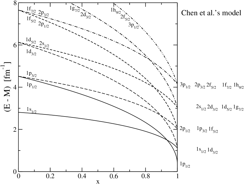
Figure 9: Single-particle spectrum in a relativistic approach with a harmonic-oscillator inspired interaction: transition from the spin-symmetry limit ($x=0$) to the pseudospin-symmetry limit ($x=1$). We limited the representation of states to those corresponding to the complete multiplets shown on the r.h.s. of the figure. Some higher-energy states are therefore not shown.

For finding solutions for the case with $\tilde{l}=l\!+\!1$ ($\kappa=-(l\!+\!1)$) and any $n$ ($ns_{1/2},\;np_{3/2},\;nd_{5/2},\;nf_{7/2},\cdots$), we notice that there is some symmetry between Eq. (12) and Eq. (13). The orbital angular momentum $l$ is replaced by $\tilde{l}$ and the solution for the small component has the same number of nodes at $x=0$ and $x=1$. What we did previously for the large component can therefore be repeated here for the small one with the appropriate replacements ($\Delta(r)\rightarrow V(r)$, $M\rightarrow-M$, $\kappa\rightarrow-\kappa$, $x\rightarrow 1-x$). Thus Eqs. (20) and (21) for $n=1$ become:

$$-\frac{\frac{dV(r)}{dr}}{E\!-\!M\!-\!V(r)}=-(1-x)\,\;\frac{\omega^{2}M}{E\!-\!M}\;\frac{(2\tilde{l}\!+\!1)\;r}{(2\tilde{l}\!+\!1\!-\!\alpha^{2}\,r^{2})}\,,$$ (25)

and:

$$E\!-\!M\!-\!V(r)=\;(E\!-\!M)\;\Big{(}1\!-\!\frac{\alpha^{2}\,r^{2}}{2\tilde{l}\!+\!1}\Big{)}^{\frac{(1\!-\!x)(2\tilde{l}\!+\!1)\omega^{2}M}{2\alpha^{2}(E\!-\!M)}}\,.$$ (26)

The general equation allowing one to determine the spectrum for any $n$ now reads:

$$E^{2}\!-\!M^{2}-(4n\!+\!2\tilde{l}\!-\!1)\;\alpha^{2}+(1\!-\!x)\,\frac{(4n\!+\!2\tilde{l}\!-\!3)\,\omega^{2}M}{E-M}=0\,.$$ (27)

The results for the spectrum are shown in Fig. 9 for $x$ varying from 0 to 1. They have been obtained using parameters identical to those used in Refs. ([23], [36]) ($M=10$ fm^-1 and $\omega=2$ fm^-1), so that to facilitate some comparison with their results. This choice also offers the advantage that the spectrum at $x=1$ is less compressed as for the choice $\omega=1$ fm^-1 used in an earlier work [22]. Examination of the figure shows that there is an one-to-one correspondence between states in the spin- and the pseudospin-symmetry limits, indicating that there is no missing states as one goes from some limit to the other one.

      

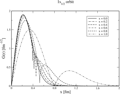
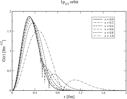
Figure 10: Appearance of an extra node in the component $G(r)$ when going from the spin- to the pseudospin-symmetry limit for orbits $1s_{1/2}$ and $1p_{3/2}$ (left and right panels respectively) with the Chen et al. model. The normalization assumes the relation $\int dr\,(G^{2}(r)+F^{2}(r))=1$.

In relation with the wave functions, we recover their expressions expected in the two symmetry limits. We find, in particular, that the large component of the states with $\tilde{l}=l\!+\!1$, corresponding to a given $n$ (as defined here by continuity with the one for the spin-symmetry case), acquires an extra node while one goes from the spin- to the pseudospin-symmetry limit. It shows that establishing a correspondence of the states with the same number of nodes in both limits, as done in Ref. [36], could lead to misleading conclusions. Actually, examination of the wave functions shows that the extra node appears at a distance where the contribution to the norm is almost saturated. This result is similar to the one obtained in the previous section for a non-relativistic model but the rate of saturation is smaller in the present case. Contributions to the norm beyond the last node amount to around 10% for the $1s_{1/2}$ state, 7% for the $1p_{3/2}$ state and less for higher angular momenta. Some results are shown in Fig. 10 for the $1s_{1/2}$ and $1p_{3/2}$ states while expressions for the wave functions can be found in the appendix A. Contrary to the nonrelativistic case, the appearance of an extra node is not progressive. Virtually, the node is present at $x=0$ but it does not show up because the factor responsible for it, $1-\frac{\alpha^{2}\,r^{2}}{2l+1}$, is taken with the power $0$, making this factor equal to 1 for any $r$ value. This is a particular feature of the transition model we used. The appearance of an extra node also holds for the small component, but only for the states with $\tilde{l}=l\!-\!1$ and when making the inverse path.

We assumed in the above study of the continuity between the spin- and pseudospin symmetry limits that the last term in Eq. (12) was linear in $x$, partly because it was the simplest possible assumption to start with. Many other assumptions could be made. A particularly attractive one for the case $\tilde{l}=l\!-\!1$ supposes to replace the factor $-x\,\frac{(2l\!+\!1)\,\omega^{2}M}{E\!+\!M}$ at the r.h.s. of Eq. (17) by $-2x\frac{(2l\!+\!3\!-\!2x)\,\alpha^{4}}{E^{2}\!-\!M^{2}}$. The dependence on $x$ of this expression is more complicated than for the choice retained here ($\alpha$ also depends on $x$), but the result for the relation between $E$ and $x$ turns out to be formally simpler. It is given by:

$$E^{2}\!-\!M^{2}=(4n\!+\!2l\!-\!1\!-\!2x)\alpha^{2}\,.$$ (28)

In writing the above result, we anticipated its generalization to any $n$. A similar result could be obtained for the case $\tilde{l}=l\!+\!1$ with the replacements of $l$ by $\tilde{l}$ and $x$ by $1-x$. It reads:

$$E^{2}\!-\!M^{2}=(4n\!+\!2l\!-\!1\!+\!2x)\alpha^{2}\,.$$ (29)

The continuous transition between the spin-and pseudospin-symmetry limits is somewhat straightforward from the above expressions. In both cases, the result should be completed by the derivation of the potentials $V(r)$ and $\Delta(r)$, which is not necessary simpler than before.

5.3 Model with $V(r)$ and $\Delta(r)$ inspired from Woods-Saxon ones

In previous sections, we examine models that were providing some continuity between the spin- and pseudospin-symmetry limits. There is no guarantee that such a continuity exists in all cases however. On the one hand, some states may disappear and reappear (or appear and disappear) in going from one limit to the other but in cases considered up to now we could find a model avoiding this drawback. On the other hand, some states may disappear (or appear), what cannot be excluded in a relativistic model where the spectrum is not bounded from below. A reason to be suspicious comes from the fact that realizing the pseudospin symmetry with a Woods-Saxon type potential supposes that its depth is larger than twice the nucleon mass, which is the obvious sign of a relativistic regime.

Figure 11: Single-particle spectrum in a relativistic approach with a Woods-Saxon inspired interaction: transition from the spin-symmetry limit ($x=0$) to the pseudospin-symmetry limit ($x=1$). Notice that our conventions for the potentials at $x=0$ and $x=1$ imply positive values for the quantity, $E-M$, represented on the vertical axis (see appendix B).

We examined various transition models from the spin-to the pseudospin-symmetry limits but, due to various problems (numerics, interpretation), we could not get clear conclusions in most cases. We present here results for one case where some interpretation is possible. Moreover, they provide interesting clues as for what could occur between the two symmetry limits. The model is described in the appendix while the spectrum is shown in Fig. 11. An essential difference with Chen et al.’s model is that the potentials at $x=0$ and $x=1$, instead of going to $\infty$ with $r$, are now limited by an upper finite value.

We first notice that the spectrum in the spin-symmetry limit looks very much like the usual one. As far as the order of the states is concerned, the spectrum in the pseudospin-symmetry limit is similar to the one for the WS model shown in Fig. 2. It would also be similar to the one obtained by Chen et al. [23], had the authors chosen to raise the degeneracy of their HO interaction model with a Woods-Saxon type correction having the opposite sign. Considering the large component of the wave functions, it is found that all states with $j=l-1/2$ and same $n$ quantum number (defined here by the order of appearance in the spectrum) have the same number of nodes in the pseudospin-symmetry limit as in the spin-symmetry limit. Instead, states with $j=l+1/2$ get an extra node, located however in a domain where the contribution to the norm beyond this node is, generally, small. This observation is similar to the one we could make for the non-relativistic case or for Chen et al.’s model [22].

At first sight, from the qualitative agreement of the spectra in the SS and PSS limits with those obtained previously in this work, we could expect similar conclusions for the spectrum between these two limits. Looking at this one however reveals important differences. It is found that there is continuity between $x=0$ and $x=1$ for all states with $j=l+1/2$, without change for the $n$ quantum number (always defined here by the order of appearance in the spectrum). This is also satisfied for states with $j=l-1/2$ and $l\geq 3$ but the picture differs for states $np_{1/2}$ and $nd_{3/2}$. As these states evolve from the spin- to the pseudospin-symmetry limit, their $n$ quantum number increases by one unit. This change is related to the appearance of an extra node in the core of the large component of the wave function. As a counterpart of the change in $n$, the states $1p_{1/2}$ and $1d_{3/2}$ in the pseudospin-symmetry limit cannot be related to any state in the spin-symmetry limit. As seen in the figure, they disappear from the spectrum around $x=0.5-0.6$, where the interaction is strongly modified. This fact explains the disappearance of the PS partner of the intruder $1s_{1/2}$ state. It is also seen on the figure that a new kind of states with $j=l+1/2$ (to whom we assign, arbitrarily, $n=0$) appears and disappears between $x=0$ and $x=1$, without spoiling the symmetry properties of the spectra obtained in these limits.

One can think, perhaps, that the extra states that appear with $E>0$ for values of $x>0$ are simple artefacts of the interaction model. However, among them, those states with $j=l-1/2$ are necessary in order the PS symmetry be satisfied for $x=1$. The other states with $j=l+1/2$ are not required by this symmetry but their appearance strongly influences the spectra of the states that are above, pushing them upwards and evidencing level-repulsion properties around $x=0.5-0.7$. Level-repulsion properties are also observed for the levels with $j=l-1/2$ in the same range. In these cases, this is the range where the wave function can be strongly changed and acquires an extra node. In some of these cases, the small and large components become comparable, suggesting the role of relativity in this change. It is noticed that, if we ignore the small region where the level-repulsion effects for these states appear, the spectra look continuous from the spin- to the pseudospin-symmetry limits. Properties of the large component of the wave function before and after the pseudo-crossing point with a similar energy are not much affected. These features are similar to the ones for the dependence of single-particle spectra as a function of the deformation of the nucleus.

The detail of the above results depends on the transition model but part of it, like the appearance of an extra node as $x$ increases as well as the appearance (or disappearance) of some states from the positive part of the SP spectrum, may point to relevant features of the models used to describe the interaction in the spin- or pseudospin-symmetry limit. Further studies could be useful to determine, in particular, whether the disappearance of states could be completely removed or, on the contrary, be extended to all states with $j=l-1/2$ and $n=1$, then providing support for the missing partners of intruder states. Whatever the picture, the results point to an important breakdown of the pseudospin symmetry. States disappear from the spectrum in one case or, in the other case, the assignment of states to pseudospin doublets differs from the one usually assumed, while agreeing with results from other parts of this work.

6 Conclusions

In this paper, we examined whether there could be some continuous transition between the spin-symmetry and the pseudospin-symmetry limit description of atomic nuclei and looked at what would be the implications of such a result. This was done by introducing an interaction that is a continuously varying superposition of potentials satisfying these symmetry properties.

Within a non-relativistic approach, we found that there could be a one-to-one correspondence between the spectra calculated in the SS and PSS limits. This is obtained with an interaction that is non-local in the PSS limit, resulting in a state ordering of the spectrum different from the one usually expected (the ground state is not necessarily a $s_{1/2}$ one). For the transition model we considered, energy shifts are larger than for the spin-orbit splitting but they do not generally exceed the splitting corresponding to two major shells. The results thus suggest to associate in the same PS doublet states $1s_{1/2}$ and $1d_{3/2}$, $1p_{3/2}$ and $1f_{5/2}$, $\cdots$, rather than states $2s_{1/2}$ and $1d_{3/2}$, $2p_{3/2}$ and $1f_{5/2}$, $\cdots$. Our suggestion is further supported by the analysis of wave functions which leads to results closer to the PS-limit expectations with our assignment than with the usual one. With this respect, we notice that wave functions for the states $1s_{1/2}$, $1p_{3/2}$, $\cdots$, get an extra node in the PSS limit but this node is located in the tail of the wave function rather than in its bulk as for states $2s_{1/2}$, $2p_{3/2}$, $\cdots$. This prevents one to identify these states together, what is further supported by our study looking at a continuous transition from the SS to the PSS limit.

We also looked at a possible continuous transition between the spectra calculated in the SS and PSS limits within a relativistic approach as this one was thought to provide some support for PSS doublets. Without regard to the origin of the interaction, we first notice that previous results can be cast into the relativistic approach by identifying the potential $V(r)$ to the one used in the non-relativistic case and taking $\Delta(r)$ as a constant. Another relativistic model is the one considered by Chen et al. [22], based on oscillator type potentials. In this case, we were able to find a potential allowing one to get a continuous transition between the SS and PSS spectra, which turn out to be very similar to those we get in the non-relativistic case. Contrary to statements made by the authors, there is no need to include intruder or missing states to make the spectra consistent with each other. We simply have to accept that the order of the states in the PSS limit differs from the usual one. With the intent to study more realistic models, we finally consider the case of finite-size potentials. Apart from the energy scale, the spectra in the SS and PSS limits were found to be similar to those obtained in the previous cases, suggesting that one could establish some continuity between them as done previously. However, while all states in the SS limit could be continuously related to states in the PSS limit, the reciprocal was not true. Some states in the PSS limit could not be related to states in the SS limit and, actually, were found to disappear from the positive-energy spectrum. Interestingly, the spectrum so obtained is found to be similar for a part to the observed one, including the assignment for PSS doublets. Thus, these results could throw light, in particular, about the disappearance of the PS partners of the intruder states when one goes from the PSS to the SS limit. The results nevertheless call for two important remarks. First, as the disappearance implies a limited number of states with $n=1$ and $j=l-1/2$, there is likely a dependence of the results on the interaction models we used in the SS and PSS limits. Second, the disappearance of states from the positive-energy spectrum points to a very strong violation of the PS symmetry in this case, more important than the one found in the other approaches where only a re-ordering of the levels was observed. Moreover, the assignment for PS doublets then implies that the large component of the wave function of one of the partners gets an extra node in its bulk when going from the SS to the PSS limit. This feature represents another violation of the PS symmetry.

From examining wave functions, it was shown in the literature that the pseudospin symmetry could not be as good as the spin one [28, 30, 32], pointing to the accidental character of the validity of this symmetry to describe the SP-level spectrum. Starting from a different viewpoint, the present results largely support this observation. If some doubt is allowed, it is due to one of the studies we performed within a relativistic framework. In this case, however, further studies could be useful to determine in what extent the results depend on specific features of the interaction we used. Either these results are confirmed and they imply, intrinsically, a very strong violation of the pseudospin symmetry, or, they confirm results of the other approaches, with a violation of this symmetry that is smaller but nevertheless larger than the spin-symmetry one.

Acknowledgments
This work has been supported by the MEC grant FIS2005-04033.

Appendix A Transition from the SS to PSS limit in the Chen et al. model

We give in this appendix some further details relative to the calculation of the spectrum between the spin- and pseudospin-symmetry limits in the Chen et al. model [22]. They successively concern the equations relating $E$ to $x$, and the parameters $\omega$ and $M$, the determination of the transition potential for the case $n=2$ and $\tilde{l}=l\!-\!1$, and, somewhat sketched, for the case $n=1$ and $\tilde{l}=l\!+\!1$.

$\bullet$ Remark about the relation of $E$ to $\omega$
It is first noticed that the equations allowing one to determine the relation of $E$ to $x$, Eqs. (24) and (27), are quadratic in $\omega$ and, therefore, apparently differ from those given in Ref. [22] in the case $x=1$ and $x=0$ respectively, which are linear in $\omega$. They can nevertheless be rearranged so that to express $\omega$ in terms of $E$ and $x$. When this is done, one recovers the expressions given in the above work:

$$\omega\,\Big{(}2n\!+\!l\!-\!\frac{3}{2}\Big{)}=\omega\,\Big{(}2n\!+\!\tilde{l}\!-\!\frac{1}{2}\Big{)}=(E\!+\!M)\,\sqrt{\frac{E\!-\!M}{2M}}\hskip 28.45274pt(\tilde{l}=l\!-\!1,\;x=1)\,,$$ (30)

$$\omega\,\Big{(}2n\!+\!\tilde{l}\!-\!\frac{3}{2}\Big{)}=\omega\,\Big{(}2n\!+\!l\!-\!\frac{1}{2}\Big{)}=(E\!-\!M)\,\sqrt{\frac{E\!+\!M}{2M}}\hskip 28.45274pt(\tilde{l}=l\!+\!1,\;x=0)\,.$$ (31)

$\bullet$ Case of states with $n=2$ and $j=l-1/2$: $2p_{1/2},\;2d_{3/2},\;2f_{5/2},\cdots$, ($\tilde{l}=l\!-\!1$)
We assumed that the wave function keeps the same form as for $x=0$ or $x=1$, $G(r)\propto r^{(l+1)}(\alpha^{2}\,r^{2}-y)\,{\rm exp}(-\alpha^{2}\,r^{2}/2)$, which implies that the last term in Eq. (12) can be written as:

$$-\frac{\frac{d\Delta(r)}{dr}(\frac{d}{dr}\!+\!\frac{\kappa}{r},\,G(r))}{E\!+\!M\!-\!\Delta(r)} = -\frac{\frac{d\Delta(r)}{dr}\;\Big{(}\alpha^{2}\,r^{2}(2l\!+\!3\!+\!y)-(2l\!+\!1)\,y-\alpha^{4}\,r^{4}\Big{)}}{(E\!+\!M\!-\!\Delta(r))\,(\alpha^{2}\,r^{2}-y)\;r}\,G(r)$$ (32)

$$= -x\,\frac{(2l\!+\!5)\,\omega^{2}M}{E\!+\!M}\frac{(\alpha^{2}\,r^{2}-z)}{(\alpha^{2}\,r^{2}-y)}\,G(r)\,.$$

The last equality is a further assumption which implies an equation to be solved:

$$-\frac{\frac{d\Delta(r)}{dr}}{E\!+\!M\!-\!\Delta(r)}=-x\,\;\frac{(2l\!+\!5)\,\omega^{2}M}{E\!+\!M}\;\frac{r\,(\alpha^{2}\,r^{2}-z)}{\Big{(}\alpha^{2}\,r^{2}(2l\!+\!3\!+\!y)-(2l\!+\!1)\,y-\alpha^{4}\,r^{4}\Big{)}}\,.$$ (33)

The quantities $y$ and $z$ are two constants that have to be determined. The first one, which corresponds to a node in the large component of the wave function, is known at $x=0$ ($y=\frac{2l+3}{2}$) and at $x=1$ ($y=\frac{2l+5}{2}$). The second one corresponds to a node in the small component of the wave function and is known at $x=1$ where it has a simple expression ($z=\frac{2l+1}{2}$). It could be chosen to simplify part of the calculations. Both $y$ and $z$ enter Eq. (12) to be solved. Looking at this equation, it is found that the coefficients of the terms proportional to $r^{l+5}$ and $r^{l-1}$ vanish with the choice we made for the wave function (using Eq. (18) in the first case and the low-$r$ behavior, $r^{l+1}$, in the second one). The vanishing of coefficients of terms $r^{l+3}$ and $r^{l+1}$ supposes the conditions:

$$E^{2}\!-\!M^{2}-(2l\!+\!7)\;\alpha^{2}+x\,\frac{(2l\!+\!5)\,\omega^{2}M}{E+M}=0\,,$$

$$(E^{2}\!-\!M^{2})\,y-(2l\!+\!3)(2+y)\,\alpha^{2}+x\,\frac{(2l\!+\!5)\,\omega^{2}M}{E+M}\;z=0\,.$$ (34)

The first of them can be cast in the general form given by Eq. (24). The second one allows one to get $y$ once a choice has been made for $z$. This last quantity enters the determination of $\Delta(r)$ and, therefore, the potential which allows one to make the transition between $x=0$ and $x=1$, where it identifies to the one used in Chen et al.’s work. A particular choice consists in taking for $z$ the value of $\alpha^{2}r^{2}$ that cancels the denominator at the r.h.s. of Eq. (33), the other value being denoted $z^{\prime}$. The value of $y,\;z,\;z^{\prime}$ so obtained are given by:

$$y = \frac{1}{8\alpha^{2}(\Delta\!E^{2}\!+\!4\alpha^{2})}\Bigg{(}(2l\!+\!3)\,((\Delta\!E^{2})^{2}+6\Delta\!E^{2}\alpha^{2}+16\alpha^{4})-(2l\!+\!1)(\Delta\!E^{2})^{2}$$

$$\hskip 85.35826pt-2\Delta\!E^{2}\sqrt{(\Delta\!E^{2}\!+\!(2l\!+\!7)\alpha^{2})^{2}+4(2l\!+\!1)(\Delta\!E^{2}\!+\!2\alpha^{2})\alpha^{2}}\Bigg{)}\,,$$

$$z = \frac{1}{8\alpha^{2}}\Bigg{(}(2l\!+\!3)(\Delta\!E^{2}+6\alpha^{2})-(2l\!+\!1)\Delta\!E^{2}$$

$$\hskip 85.35826pt-2\sqrt{(\Delta\!E^{2}\!+\!(2l\!+\!7)\alpha^{2})^{2}+4(2l\!+\!1)(\Delta\!E^{2}\!+\!2\alpha^{2})\alpha^{2}}\Bigg{)}\,,$$

$$z^{\prime} = 2l+3+y-z$$ (35)

$$= \frac{1}{2(\Delta\!E^{2}\!+\!4\alpha^{2})}\Bigg{(}(2l\!+\!3)(\Delta\!E^{2}+6\alpha^{2})+(2l\!+\!1)\Delta\!E^{2}$$

$$\hskip 85.35826pt+2\sqrt{(\Delta\!E^{2}\!+\!(2l\!+\!7)\alpha^{2})^{2}+4(2l\!+\!1)(\Delta\!E^{2}\!+\!2\alpha^{2})\alpha^{2}}\Bigg{)}\,,$$

where $\Delta\!E^{2}=E^{2}\!-\!M^{2}-(2l\!+\!7)\alpha^{2}=-x\,\frac{(2l\!+\!5)\,\omega^{2}M}{E+M}$ ($\Delta\!E^{2}=0$ at $x=0$ and $\Delta\!E^{2}=-2$ at $x=1$). The quantity $\Delta(r)$ can then be calculated easily from the following equation:

$$-\frac{\frac{d\Delta(r)}{dr}}{E\!+\!M\!-\!\Delta(r)}=-x\,\;\frac{\omega^{2}M}{E\!+\!M}\;\frac{(2l\!+\!5)\;r}{(z^{\prime}\!-\!\alpha^{2}\,r^{2})}$$ (36)

The solution takes a relatively simple form. It is similar to Eq. (21) for the $n=1$ case and is given by:

$$E\!+\!M\!-\!\Delta(r)=\;(E\!+\!M)\;\Big{(}1\!-\!\frac{\alpha^{2}r^{2}}{z^{\prime}}\Big{)}^{\frac{x(2l\!+\!5)\omega^{2}M}{2\alpha^{2}(E\!+\!M)}}\,.$$ (37)

It can be checked that the exponent is equal to 1 at $x=1$, so that the factor at the denominator in Eq. (32) exactly cancels a similar factor $(z^{\prime}\!-\!\alpha^{2}r^{2})$ at the numerator (up to a constant factor).

The solution for the small component is given by:

$$F(r)=\frac{(\frac{d}{dr}\!+\!\frac{\kappa}{r},\,G(r))}{E\!+\!M\!-\!\Delta(r)}=\frac{(2l\!+\!1)}{E\!+\!M}\;\Big{(}1\!-\!\frac{\alpha^{2}r^{2}}{z^{\prime}}\Big{)}^{(1-\frac{x(2l\!+\!5)\omega^{2}M}{2\alpha^{2}(E\!+\!M)})}\;\frac{(1-\frac{\alpha^{2}r^{2}}{z})\,G(r)}{(1-\frac{\alpha^{2}r^{2}}{y})\,r}\,.$$ (38)

$\bullet$ Case of states with $n=1$ and $j=l+1/2$: $1s_{1/2},\;1p_{3/2},\;1d_{5/2},\;1f_{7/2},\cdots$, ($\tilde{l}=l\!+\!1$)
The solution we retained in this case has been obtained from the observation that there is some symmetry between Eq. (12) for the large component and Eq. (13) for the small one. Most developments presented in the main text for the case ($\tilde{l}=l\!+\!1$) can thus be transposed here. For the case with $n=1$, we therefore look for a small component with the following form $F(r)\propto r^{(\tilde{l}+1)}\,{\rm exp}(-\alpha^{2}\,r^{2}/2)\propto r^{(l+2)}\,{\rm exp}(-\alpha^{2}\,r^{2}/2)$, which is common to the expected solutions at $x=0$ and $x=1$. The solution for the large component can be obtained using its expression in term of the small one together with the expression of the transition potential given by Eq. (26):

$$G(r)=-\frac{(\frac{d}{dr}\!-\!\frac{\kappa}{r},\,F(r))}{E\!-\!M\!-\!V(r)}=-\frac{2\tilde{l}\!+\!1}{E\!-\!M}\;\Big{(}1\!-\!\frac{\alpha^{2}\,r^{2}}{2\tilde{l}\!+\!1}\Big{)}^{(1-\frac{(1\!-\!x)(2\tilde{l}\!+\!1)\omega^{2}M}{2\alpha^{2}(E\!-\!M)})}\;\;\frac{F(r)}{r}\,.$$ (39)

The above solution is consistent with the idea that the spin symmetry results from the cancellation of $\Delta(r)$ while the pseudospin symmetry results from the cancellation of $V(r)$, without any regard to the smallness of one component with respect to the other one. Solutions that are more in agreement with this last observation have also been found. They nevertheless differ from the solutions presented in the main text with many respects. The equation allowing one to determine $E$ as a function of $x$ is more complicated but the appearance of a node for the large component is more progressive. On the other hand, some modification of the normalization, that can be actually justified, is necessary to make it convergent.

Appendix B Transition from the SS to PSS limit in a relativistic model with finite potentials

In order to study the transition between two models A and B satisfying exact SS and PSS, respectively, we consider, in accordance with the definitions given in Subsect. 5.1, the potentials $V(r)=\Sigma_{v}(r)+\Sigma_{s}(r)$ and $\Delta(r)=\Sigma_{v}(r)-\Sigma_{s}(r)$ entering the Dirac equation (11):

$$V(r)=(1-x)\frac{8M}{1+e^{-(r-r_{0})/a}}\left[\frac{1}{1+e^{(r-r_{0})/a}}+\eta\frac{1}{1+e^{-(r-r_{0})/a}}\right],$$ (40)

$$\Delta(r)=x\frac{4M}{1+e^{-(r-r_{0})/a}},$$ (41)

where, we take, somewhat arbitrarily, $a=0.1$, $M=10$ fm^-1, $r_{0}=2$ fm, and

$$\eta=\frac{4(x_{0}-x)}{1+100(x-x_{0})^{2}},$$ (42)

with (see below)

$$x_{0}=\frac{E+M}{4M}.$$ (43)

Thus, for $x=0$ we recover the model A, which satisfies the exact spin symmetry, whereas for $x=1$, we have the model B, which satisfies the exact pseudospin symmetry. We do not think our main conclusions will depend very much on our specific election of parameters. Like for Chen et al.’s model [22], the strengths of the potential $V(r)$ at $x=0$ and $\Delta(r)$ at $x=1$ are small in the vicinity of $r=0$. In the large-$r$ limit, they are however bounded by an upper finite value instead to increase infinitely. The value of $e=E-M$ is then necessarily positive at $x=0$ or $x=1$. In what follows, we may omit, by simplicity, the explicit dependence of $V(r)$ and $\Delta(r)$ on the space coordinate $r$.

To facilitate the understanding of the solutions of the Dirac equation (11) with these potentials, it is useful to consider the corresponding equivalent Schrödinger equation for the large component (see Ref. [32] for details). In this equation, with the potential $\Delta$ that becomes constant for $r\rightarrow\infty$, the central potential ($U(r)\equiv U$) at $r\rightarrow\infty$ can be approximated as

$$U(r\rightarrow\infty)=V+\frac{1}{2M}\left[e(V+\Delta)-e^{2}-V\Delta\right],$$ (44)

where $e\equiv E-M$.

The last term in Eq. (40), $\propto\eta$, makes $V(r\rightarrow\infty)$ different from zero. Its sign changes at $x=x_{0}$ to make the central potential $U(r)$ attractive at large values of $r$. The factor 4 entering the expression of $\eta$ controls the “speed” of the transition from the SS to the PSS limit as $x$ varies. The factor $100$ (together with the factor $4$) determines the value of $V$ at $r\rightarrow\infty$ for a given value of $x$.

The potential $V(r\rightarrow\infty)$ can be written in terms of $U$ and $\Delta$ as,

$$V(r\rightarrow\infty)=\frac{2M(U/e)-(\Delta-e)}{2M-(\Delta-e)}e.$$ (45)

Notice that $x_{0}$ is the value of $x$ for which the denominator $2M-(\Delta-e)=0$. The potential $V$ is chosen so that it remains always finite at $r\rightarrow\infty$, in particular for $x=x_{0}$. In this case, necessarily, $U(r\rightarrow\infty)=e$ for $x=x_{0}$. Thus, the system for $x\rightarrow x_{0}$ spreads all over the space. However, with the choice for the potentials $V$ and $\Delta$, it is possible to find bound states for $x$ very close to $x_{0}$ and, in most of cases, the SP energies vary smoothly with $x$ around $x_{0}$. Only when the value of the SP-state energy is high enough and $x_{0}$ approaches the true value of $x$, for which the transition from the SS to the PSS limit is produced, in practice, the SP energy may vary quite sharply for states with $l$ large and $j=l-1/2$ (see the SP energies for the states $f_{5/2}$ and $g_{7/2}$ in Fig. 11).

References

- [1] A. Arima, M. Harvey, K. Shimizu, Phys. Lett. B 30, 517 (1969).
- [2] K.T. Hecht, A. Adler, Nucl. Phys. A 137, 129 (1969).
- [3] A. Bohr, I. Hamamoto and Ben R. Mottelson, Physica Scripta 26, 267 (1982).
- [4] C. Bahri, J.P. Draayer and S.A. Moszkowski, Phys. Rev. Lett. 68, 2135 (1992).
- [5] O. Castaños, M. Moshinsky and C. Quesne, Phys. Lett. B 277, 238 (1992).
- [6] J.N. Ginocchio, Phys. Rev. Lett. 78, 436 (1997).
- [7] J.D. Walecka, Ann of Phys. (N.Y.) 83, 491 (1974).
- [8] A. Bouyssy, S. Marcos and Pham Van Thieu, Nucl. Phys. A422, 541 (1984).
- [9] B.D. Serot and J.D. Walecka, in Advances in Nuclear Physics 16, edited by J.W. Negele and E. Vogt, (Plenum, N.Y., 1986).
- [10] P. A. M. Dirac, Proc. Roy. Soc. (London), A117, 610 (1928); A118, 351 (1928).
- [11] J.N. Ginocchio, D.G. Madland, Phys. Rev. C 57, 1167 (1998).
- [12] J.N. Ginocchio, Phys. Rev. C 59, 2487 (1999); Phys. Rev. Lett. 82, 4599 (1999); Phys. Rep. 315, 231 (1999); J. Phys. G.: Nucl. Part. Phys. 25, 617 (1999).
- [13] J.N. Ginocchio, A. Leviatan, Phys. Rev. Lett. 87, 072502 (2001).
- [14] A. Leviatan, J.N. Ginocchio, Phys. Lett. B 518, 214 (2001).
- [15] J.N. Ginocchio, Phys. Rep. 414, 165 (2005); Nucl. Phys. News 15, 13 (2005).
- [16] Y.K. Gambhir, J.P. Maharana and C.S. Warke, Eur. Phys. J. A 3, 255 (1998).
- [17] G.A Lalazissis, Y.K. Gambhir, J.P. Maharana, C.S. Warke, P. Ring, Phys. C 58, R45 (1998).
- [18] J. Meng, K. Sugawara-Tanabe, S. Yamaji, P. Ring, A. Arima, Phys. Rev. C 58, R628 (1998).
- [19] K. Sugawara-Tanabe, A. Arima, Phys. Rev. C 58, R3065 (1998).
- [20] J. Meng, K. Sugawara-Tanabe, S. Yamaji, A. Arima, Phys. Rev. C 59, 154 (1999).
- [21] K. Sugawara-Tanabe, J. Meng, S. Yamaji, A. Arima, J. Phys. G: Nucl. Part. Phys. 25, 811 (1999).
- [22] T. S. Chen et al., nucl-th/0205021
- [23] T.S. Chen, H.F. Lü, J. Meng, S.O. Zhang, and S.G. Zhou, Chin. Phys. Lett. 20, 358 (2003).
- [24] W. Hui Long, H. Sagawa, J. Meng and N. Van Giai, Phys. Lett. B 639, 242 (2006).
- [25] S. Marcos, L.N. Savushkin, M. López-Quelle, P. Ring, Phys. Rev. C 62, 054309 (2000).
- [26] S. Marcos, M. López-Quelle, R. Niembro, L.N. Savushkin, P. Bernardos, Phys. Lett. B 513, 30 (2001).
- [27] S. Marcos, M. López-Quelle, R. Niembro, L.N. Savushkin, P. Bernardos, Eur. Phys. J. A 17, 173 (2003).
- [28] S. Marcos, M. López-Quelle, R. Niembro, L.N. Savushkin, Eur. Phys. J. A 20, 443 (2004).
- [29] S. Marcos, M. López-Quelle, R. Niembro, L.N. Savushkin, J. Phys G: Nucl. Part. Phys. 31, S1551 (2005).
- [30] S. Marcos, V.N. Fomenko, M. López-Quelle, R. Niembro, L.N. Savushkin, Eur. Phys. J. A 26, 253 (2005).
- [31] S. Marcos, M. López-Quelle, R. Niembro, L.N. Savushkin, Eur. Phys. J. A 34, 429 (2007).
- [32] S. Marcos, M. López-Quelle, R. Niembro, L.N. Savushkin, Eur. Phys. J. A 37, 251 (2008).
- [33] P. Alberto, M. Fiolhais, M. Malheiro, A. Delfino, M. Chiapparini, Phys. Rev. Lett. 86, 5015 (2001).
- [34] P. Alberto, M. Fiolhais, M. Malheiro, A. Delfino, M. Chiapparini, Phys. Rev. C 65, 034307 (2002).
- [35] R. Lisboa, M. Malheiro, P. Alberto, Phys. Rev. C 67, 054305 (2003).
- [36] R. Lisboa, M. Malheiro, A.S. de Castro, P. Alberto, M. Fiolhais, Phys. Rev. C 69, 024319 (2004).
- [37] M. López-Quelle, L.N. Savushkin, S. Marcos, P. Bernardos, R. Niembro, Nucl. Phys. A 727, 269 (2003).
- [38] M. López-Quelle, S. Marcos, L.N. Savushkin, R. Niembro, Recent Res. Devel. Physics 6, 29 (2005).
- [39] M. López-Quelle, L.N. Savushkin, S. Marcos and R. Niembro, J. Phys G: Nucl. Part. Phys. 31, S1911 (2005).
- [40] A. L. Blockhin, C. Bahri and J. P. Draayer, Phys. Rev. Lett. 74, 4149 (1995).