Model-free control and intelligent PID controllers: towards a possible trivialization of nonlinear control?

Abstract

.  We are introducing a model-free control and a control with a restricted model for finite-dimensional complex systems. This control design may be viewed as a contribution to “intelligent” PID controllers, the tuning of which becomes quite straightforward, even with highly nonlinear and/or time-varying systems. Our main tool is a newly developed numerical differentiation. Differential algebra provides the theoretical framework. Our approach is validated by several numerical experiments.

1 Introduction

Writing down simple and reliable differential equations for describing a concrete plant is almost always a daunting task. How to take into account, for instance, frictions, heat effects, ageing processes, characteristics dispersions due to mass production, …? Those severe difficulties explain to a large extent why the industrial world is not willing to employ most techniques stemming from “modern” control theory, which are too often based on a “precise” mathematical modeling, in spite of considerable advances during the last fifty years. We try here to overcome this unfortunate situation thanks to recent fast estimation methods. Two cases are examined:

1. Model-free control is based on an elementary continuously updated local modeling via the unique knowledge of the input-output behavior. It should not be confused with the usual “black box” identification (see, e.g., (Kerschen, Worden, Vakakis & Golinval (2006); Sjöberg, Zhang, Ljung, Benveniste, Delyon, Glorennec, Hjalmarsson & Juditsky (1995))), where one is looking for a model which is valid within an operating range which should be as large as possible. Let us summarize our approach in the monovariable case. The input-output behavior of the system is assumed to “approximatively” governed within its operating range by an unknown finite-dimensional ordinary differential equation, which is not necessarily linear,

   $$E(y,\dot{y},\dots,y^{(a)},u,\dot{u},\dots,u^{(b)})=0$$ (1)

   We replace Eq. (1) by the following “phenomenological” model, which is only valid during a very short time interval,

   $$y^{(\nu)}=F+\alpha u$$ (2)

   The derivation order $\nu$, which is in general equal to $1$ or $2$, and the constant parameter $\alpha$ are chosen by the practitioner. It implies that $\nu$ is not necessarily equal to the derivation order $a$ of $y$ in Eq. (1). The numerical value of $F$ at any time instant is deduced from those of $u$ and $y^{(\nu)}$, thanks to our numerical differentiators (Fliess, Join & Sira-Ramírez (2008); Mboup, Join & Fliess (2009)). The desired behavior is obtained by implementing, if, for instance, $\nu=2$, the intelligent PID controller (i-PID)

   $$u=-\frac{F}{\alpha}+\frac{\ddot{y}^{\ast}}{\alpha}+K_{P}e+K_{I}\int e+K_{D}\dot{e}$$ (3)

   where

   • $y^{\ast}$ is the output reference trajectory, which is determined via the rules of flatness-based control (see, e.g., Fliess, Lévine, Martin & Rouchon (1995); Rotella & Zambettakis (2007); Sira-Ramírez & Agrawal (2004));

   • $e=y-y^{\ast}$ is the tracking error;

   • $K_{P}$, $K_{I}$, $K_{D}$ are the usual tuning gains.

2. Assume now that a restricted or partial model of the plant is quite well known and is defined by Eq. (1) for instance. The plant is then governed by the restricted, or incomplete, modeling,

   $$E(y,\dot{y},\dots,y^{(a)},u,\dot{u},\dots,u^{(b)})+G=0$$

   where $G$ stands for all the unknown parts. If the known system, which corresponds to $E=0$, is flat, we also easily derive an intelligent controller, or i-controller, which gets rid of the unknown effects.

Differential algebra is briefly reviewed in Sect. 2 in order to

• derive the input-output differential equations,

• define minimum and non-minimum phase systems.

Numerical differentiation of noisy signals is examined in Sect. 3. Sect. 4 states the basic principles of our model-free control. Several numerical experiments are reported in Sect. 5. We deal as well with linear and nonlinear systems and with monovariable and multivariable systems. An anti-windup strategy is sketched in Sect. 5.4.2. Sect. 6 studies the control with a partially known medeling. One of the two examples deals with a non-minimum phase system. The numerical simulations of Sect. 5.1 and Sect. 6.2 show the that our controllers behave much better than classic PIDs. Several concluding remarks are discussed in Sect. 7.

Remark 1

Only Sect. 2 is written in an abstract algebraic language. In order to understand the sequel and, in particular, the basic principles of our control strategy, it is only required to admit the input-output representations (1) and (4), as well as the foundations of flatness-based control (Fliess, Lévine, Martin & Rouchon (1995); Rotella & Zambettakis (2007); Sira-Ramírez & Agrawal (2004)).

2 Nonlinear systems

2.1 Differential fields

All the fields considered here are commutative and have characteristic $0$. A differential field $\mathfrak{K}$ is a field which is equipped with a derivation $\frac{d}{dt}$, i.e., a mapping $\mathfrak{K}\rightarrow\mathfrak{K}$ such that, $\forall\leavevmode\nobreak\ a,b\in\mathfrak{K}$,

• $\frac{d}{dt}(a+b)=\dot{a}+\dot{b}$,

• $\frac{d}{dt}(ab)=\dot{a}b+a\dot{b}$.

A constant $c\in\mathfrak{K}$ is an element such that $\dot{c}=0$. The set of all constant elements is the subfield of constants.

A differential field extension $\mathfrak{L}/\mathfrak{K}$ is defined by two differential fields $\mathfrak{K}$, $\mathfrak{L}$ such that:

• ${\mathfrak{K}}\subseteq{\mathfrak{L}}$,

• the derivation of $\mathfrak{K}$ is the restriction to $\mathfrak{K}$ of the derivation of $\mathfrak{L}$.

Write ${\mathfrak{K}}\langle S\rangle$, $S\subset{\mathfrak{L}}$, the differential subfield of $\mathfrak{L}$ generated by $\mathfrak{K}$ and $S$. Assume that $\mathfrak{L}/\mathfrak{K}$ is finitely generated, i.e., ${\mathfrak{L}}={\mathfrak{K}}\langle S\rangle$, where $S$ est finite. An element $\xi\in\mathfrak{L}$ is said to be differentially algebraic over $\mathfrak{K}$ if, and only if, it satisfies an algebraic differential equation $P(\xi,\dots,\xi^{(n)})=0$, where $P$ is a polynomial function over $\mathfrak{K}$ in $n+1$ variables. The extension $\mathfrak{L}/\mathfrak{K}$ is said to be differentially algebraic if, and only if, any element of $\mathfrak{L}$ is differentially algebraic over $\mathfrak{K}$. The next result is important:
$\mathfrak{L}/\mathfrak{K}$ is differentially algebraic if, and only if, its transcendence degree is finite.

An element of $\mathfrak{L}$, which is non-differentially algebraic over $\mathfrak{K}$, is said to differentially transcendental over $\mathfrak{K}$. An extension $\mathfrak{L}/\mathfrak{K}$, which is non-differentially algebraic, is said to be differentially transcendental. A set $\{\xi_{\iota}\in\mathfrak{L}\mid\iota\in I\}$ is said to be differentially algebraically independent over $\mathfrak{K}$ if, and only if, there does not exists any non-trivial differential relation over $\mathfrak{K}$:
$Q(\dots,\xi_{\iota}^{(\nu_{\iota})},\dots)=0$, where $Q$ is a polynomial function over $\mathfrak{K}$, implies $Q\equiv 0$.
Two such sets, which are maximal with respect to set inclusion, have the same cardinality, i.e., they have the same number of elements: this is the differential transcendence degree of the extension $\mathfrak{L}/\mathfrak{K}$. Such a set is a differential transcendence basis. It should be clear that ${\mathfrak{L}}/{\mathfrak{K}}$ is differentially algebraic if, and only if, its differential transcendence degree is $0$.

2.2 Nonlinear systems

2.2.1 General definitions

Let $k$ be a given differential ground field. A system is a finitely generated differentially transcendental extension ${\mathcal{K}}/k$. Let $m$ be its differential transcendence degree. A set of (independent) control variables ${\boldsymbol{u}}=(u_{1},\dots,u_{m})$ is a differential transcendence basis of ${\mathcal{K}}/k$. The extension ${\mathcal{K}}/k\langle\boldsymbol{u}\rangle$ is therefore differentially algebraic. A set of output variables ${\boldsymbol{y}}=(y_{1},\dots,y_{p})$ is a subset of ${\mathcal{K}}$.

Let $n$ be the transcendence degree of ${\mathcal{K}}/k\langle\boldsymbol{u}\rangle$ and let ${\boldsymbol{x}}=(x_{1},\dots,x_{n})$ be a transcendence basis of this extension. It yields the generalized state representation:

$$\begin{array}[]{l}A_{\iota}(\dot{x}_{\iota},{\boldsymbol{x}},{\boldsymbol{u}},\dots,{\boldsymbol{u}}^{(\alpha)})=0\\ B_{\kappa}(y_{\kappa},{\boldsymbol{x}},{\boldsymbol{u}},\dots,{\boldsymbol{u}}^{(\beta)})=0\end{array}$$

where $A_{\iota}$, $\iota=1,\dots,n$, $B_{\kappa}$, $\kappa=1,\dots,p$, are polynomial functions over $k$.

The following input-output representation is a consequence from the fact that $y_{1},\dots,y_{p}$ are differentially algebraic over $k\langle{\mathbf{u}}\rangle$:

$$\Phi_{j}({\boldsymbol{y}},\dots,{\boldsymbol{y}}^{(\bar{N}_{j})},{\boldsymbol{u}},\dots,{\boldsymbol{u}}^{(\bar{M}_{j})})=0$$ (4)

where $\Phi_{j}$, $j=1,\dots,p$, is a polynomial function over $k$.

2.2.2 Input-output invertibility

• The system is said to be left invertible if, and only if, the extension $k\langle{{\boldsymbol{u}},\boldsymbol{y}}\rangle/k\langle{\boldsymbol{y}}\rangle$ is differentially algebraic. It means that one can compute the input variables from the output variables via differential equations. Then $m\leq p$.

• It is said to be right invertible if, and only if, the differential transcendence degree of $k\langle{\boldsymbol{y}}\rangle/k$ is equal to $p$. This is equivalent saying that the output variables are differentially algebraically independent over $k$. Then $p\leq m$.

The system is said to be square if, and only if, $m=p$. Then left and right invertibilities coincide. If those properties hold true, the system is said to be invertible.

2.2.3 Minimum and non-minimum phase systems

The ground field $k$ is now the field $\mathbb{R}$ of real numbers. Assume that our system is left invertible. The stable or unstable behavior of Eq. (4), when considered as a system of differential equations in the unknowns ${\boldsymbol{u}}$ (${\boldsymbol{y}}$ is given) yields the definition of minimum, or non-minimum, phase systems (compare with Isidori (1999)).

3 Numerical differentiation

The interested reader will find more details and references in (Fliess, Join & Sira-Ramírez (2008)). We refer to (Mboup, Join & Fliess (2009)) for crucial developments which play an important rôle in practical implementions.

3.1 General principles

3.1.1 Polynomial signals

Consider the polynomial time function of degree $N$

$$x_{N}(t)=\sum_{\nu=0}^{N}x^{(\nu)}(0)\frac{t^{\nu}}{\nu!}$$

where $t\geq 0$. Its operational, or Laplace, transform (see, e.g., Yosida (1984)) is

$$X_{N}(s)=\sum_{\nu=0}^{N}\frac{x^{(\nu)}(0)}{s^{\nu+1}}$$ (5)

Introduce $\frac{d}{ds}$, which is sometimes called the algebraic derivation. Multiply both sides of Eq. (5) by $\frac{d^{\alpha}}{ds^{\alpha}}s^{N+1}$, $\alpha=0,1,\dots,N$. The quantities $x^{(\nu)}(0)$, $\nu=0,1,\dots,N$, which satisfy a triangular system of linear equations, with non-zero diagonal elements,

$$\frac{d^{\alpha}s^{N+1}X_{N}}{ds^{\alpha}}=\frac{d^{\alpha}}{ds^{\alpha}}\left(\sum_{\nu=0}^{N}x^{(\nu)}(0)s^{N-\nu}\right)$$ (6)

are said to be linearly identifiable (Fliess & Sira-Ramírez (2003)). One gets rid of the time derivatives $s^{\mu}\frac{d^{\iota}X_{N}}{ds^{\iota}}$, $\mu=1,\dots,N$, $0\leq\iota\leq N$, by multiplying both sides of Eq. (6) by $s^{-\bar{N}}$, $\bar{N}>N$.

Remark 2

The correspondence between $\frac{d^{\alpha}}{ds^{\alpha}}$ and the product by $(-t)^{\alpha}$ (see, e.g., Yosida (1984)) permits to go back to the time domain.

3.1.2 Analytic signals

A time signal is said to be analytic if, and only if, its Taylor expansion is convergent. Truncating this expansion permits to apply the previous calculations.

3.2 Noises

Noises are viewed here as quick fluctuations around $0$. They are therefore attenuated by low-pass filters, like iterated integrals with respect to time.

4 Model-free control: general principles

It is impossible of course to give here a complete description which would trivialize for practitioners the implementation of our control design. We hope that numerous concrete applications will make such an endeavor feasible in a near future.

4.1 Local modeling

1. Assume that the system is left invertible. If there are more output variables than input variable, i.e., $p\gneqq m$, pick up $m$ output variables, say the first $m$ ones, in order to get an invertible square system. Eq. (2) may be extended by writing

   $$\begin{array}[]{l}y^{(n_{1})}_{1}=F_{1}+\alpha_{1,1}u_{1}+\dots+\alpha_{1,m}u_{m}\\ \ldots\\ y^{(n_{p})}_{p}=F_{m}+\alpha_{m,1}u_{1}+\dots+\alpha_{p,m}u_{m}\end{array}$$ (7)

   where

   • $n_{j}\geq 1$, $j=1,\dots,p$, and, most often, $n_{j}=1$ or $2$;

   • $\alpha_{j,i}\in\mathbb{R}$, $i=1,\dots,m$, $j=1,\dots,p$, are non-physical constant parameters, which are chosen by the pratitioner such that $\alpha_{j,i}u_{i}$ and $F_{j}$ are of the same magnitude.

2. In order to avoid any algebraic loop, the numerical value of

   $$F_{j}=y^{(n_{j})}_{j}-\alpha_{j,1}u_{1}-\dots-\alpha_{j,m}u_{m}$$

   is given thanks to the time sampling

   $$F_{j}(\kappa)=[y^{(n_{j})}_{j}(\kappa)]_{e}-\sum_{i=1}^{m}\alpha_{j,i}u_{i}(\kappa-1)$$

   where $[\bullet(\kappa)]_{e}$ stands for the estimate at the time instant $\kappa$.

3. The determination of the reference trajectories for the output variables $y_{j}$ is achieved in the same way as in flatness-based control.

Remark 3

It should also be pointed out that, in order to avoid algebraic loops, it is necessary that in Eq. (4)

$$\frac{\partial\Phi_{j}}{\partial y_{j}^{(n_{j})}}\not\equiv 0,\quad\leavevmode\nobreak\ j=1,\dots,p$$

It yields

$$n_{j}\leq\bar{N}_{j}$$

Numerical instabilities might appear when $\frac{\partial\Phi_{j}}{\partial y_{j}^{(n_{j})}}$ is closed to $0$.

Remark 4

Our control design lead with non-minimum phase systems to divergent numerical values for the control variables $u_{j}$ and therefore to the inapplicability of our techniques.

Remark 5

Remember that the Equations (1) and (4) are unknown. Verifying therefore the properties discussed in the two previous remarks may only be achieved experimentally within the plant operating range.

4.2 Controllers

Let us restrict ourselves for the sake of notations simplicity to monovariable systems. If $\nu=2$ in Eq. (2), the intelligent PID controller has already been defined by Eq. (3). If $\nu=1$ in Eq. (2), replace Eq. (3) by the intelligent PI controller, or i-PI,

$$u=-\frac{F}{\alpha}+\frac{\dot{y}^{\ast}}{\alpha}+K_{P}e+K_{I}\int e$$ (8)

Remark 6

Until now we were never obliged to chose $\nu\gvertneqq 2$ in Eq. (2). The previous controllers (3) and (8) might then be easily extended to to the generalized proportional integral controllers, or GPIs, of (Fliess, Marquez, Delaleau & Sira-Ramírez (2002)).

Remark 7

In order to improve the performances it might be judicious to replace in Eq. (3) or in Eq. (8) the unique integral term $K_{I}\int e$ by a finite sum of iterated integrals

$$K_{I_{1}}\int e+K_{I_{2}}\int\int e+\dots+K_{I_{\Lambda}}\int\dots\int e$$

where

• $\int\dots\int e$ stands for the iterated integral of order $\Lambda$,

• the $K_{I_{\lambda}}$, $\lambda=1,\dots,\Lambda$, are gains.

We get if $K_{I_{\Lambda}}\neq 0$ an intelligent PI^ΛD or PI^Λ controller. Note also that setting $\Lambda=0$ is a mathematical possibility. The lack of any integral term is nevertheless not recommended from a practical viewpoint.

Let us briefly compare our intelligent PID controllers to classic PID controllers:

• We do not need any identification procedure since the whole structural information is contained in the term $F$ of Eq. (2), which is eliminated thanks to Eq. (3).

• The reference trajectories, which are chosen thanks to flatness-based methods, is much more flexible than the trajectories which are usually utilized in the industry. Overshoots and undershoots are therefore avoided to a large extent.

5 Some examples of model-free control

A zero-mean Gaussian white noise of variance $0.01$ is added to all the computer simulations in order to test the robustness property of our control design. We utilize a standard low-pass filter with classic controllers and the principles of Sect. 3.2 with our intelligent controllers.

5.1 A stable monovariable linear system

The transfer function

$$\frac{(s+2)^{2}}{(s+1)^{3}}$$ (9)

defines a stable monovariable linear system.

5.1.1 A classic PID controller

We apply the well known method due to Broïda (see, e.g., Dindeleux (1981)) by approximating the system (9) via the following delay system

$$\frac{Ke^{-\tau s}}{(Ts+1)}$$

$K=4$, $T=2.018$, $\tau=0.2424$ are obtained thanks to graphical techniques. The gain of the PID controller are then deduced (Dindeleux (1981)): $K_{P}=\frac{100(0.4\tau+T)}{120K\tau}=1.8181$, $K_{I}=\frac{1}{1.33K\tau}=0.7754$, $K_{D}=\frac{0.35T}{K}=0.1766$.

5.1.2 i-PI.

We are employing $\dot{y}=F+u$ and the i-PI controller

$$u=-[F]_{e}+\dot{y}^{\star}+\mbox{\rm PI}(e)$$

where

• $[F]_{e}=[\dot{y}]_{e}-u$,

• $y^{\star}$ is a reference trajectory,

• $e=y-y^{\star}$,

• $\mbox{\rm PI}(e)$ is an usual PI controller.

5.1.3 Numerical simulations

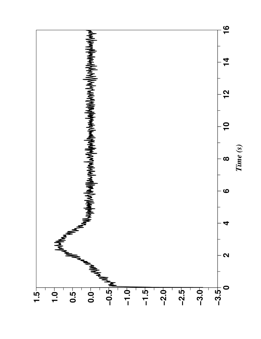
(a) i-PI control

(b) Output (–); reference (- -); denoised output (. .)

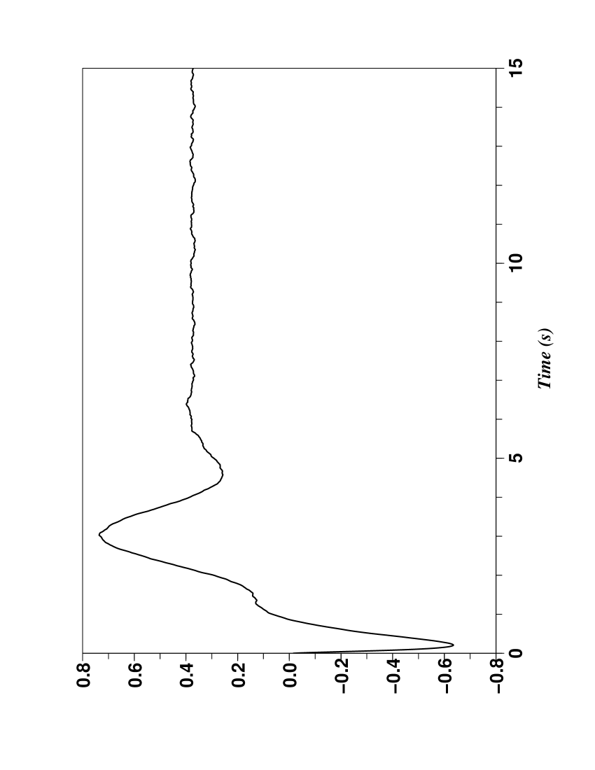
(c) PID control

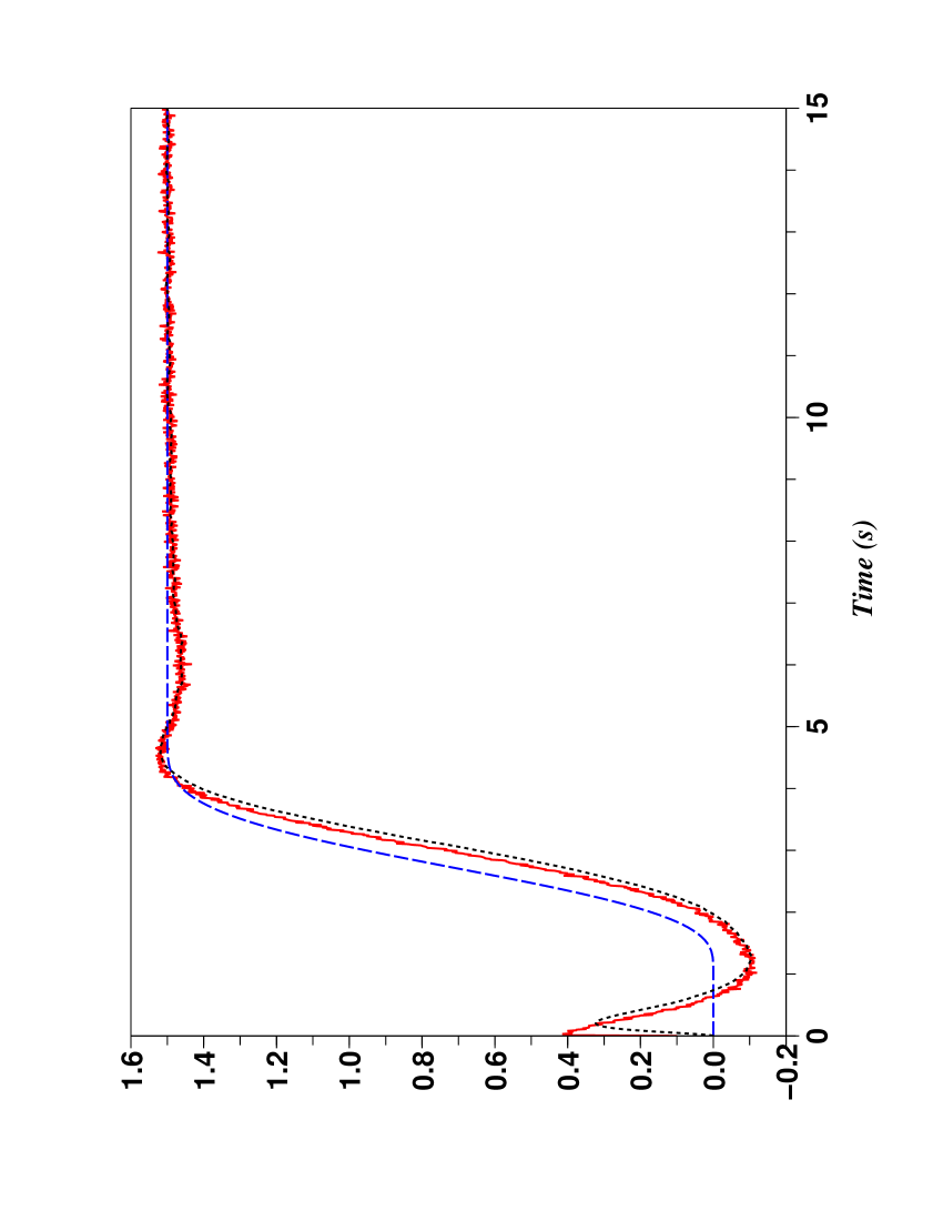
(d) Output (–); reference (- -); denoised output (. .)

Figure 1: Stable linear monovariable system

Fig. 1 shows that the i-PI controller behaves only slightly better than the classic PID controller. When taking into account on the other hand the ageing process and some fault accommodation there is a dramatic change of situation:

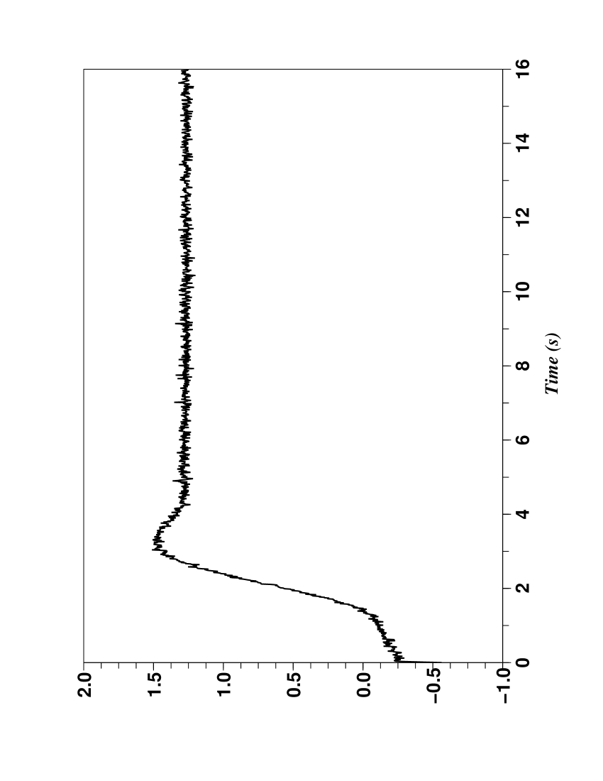
(a) i-PI control

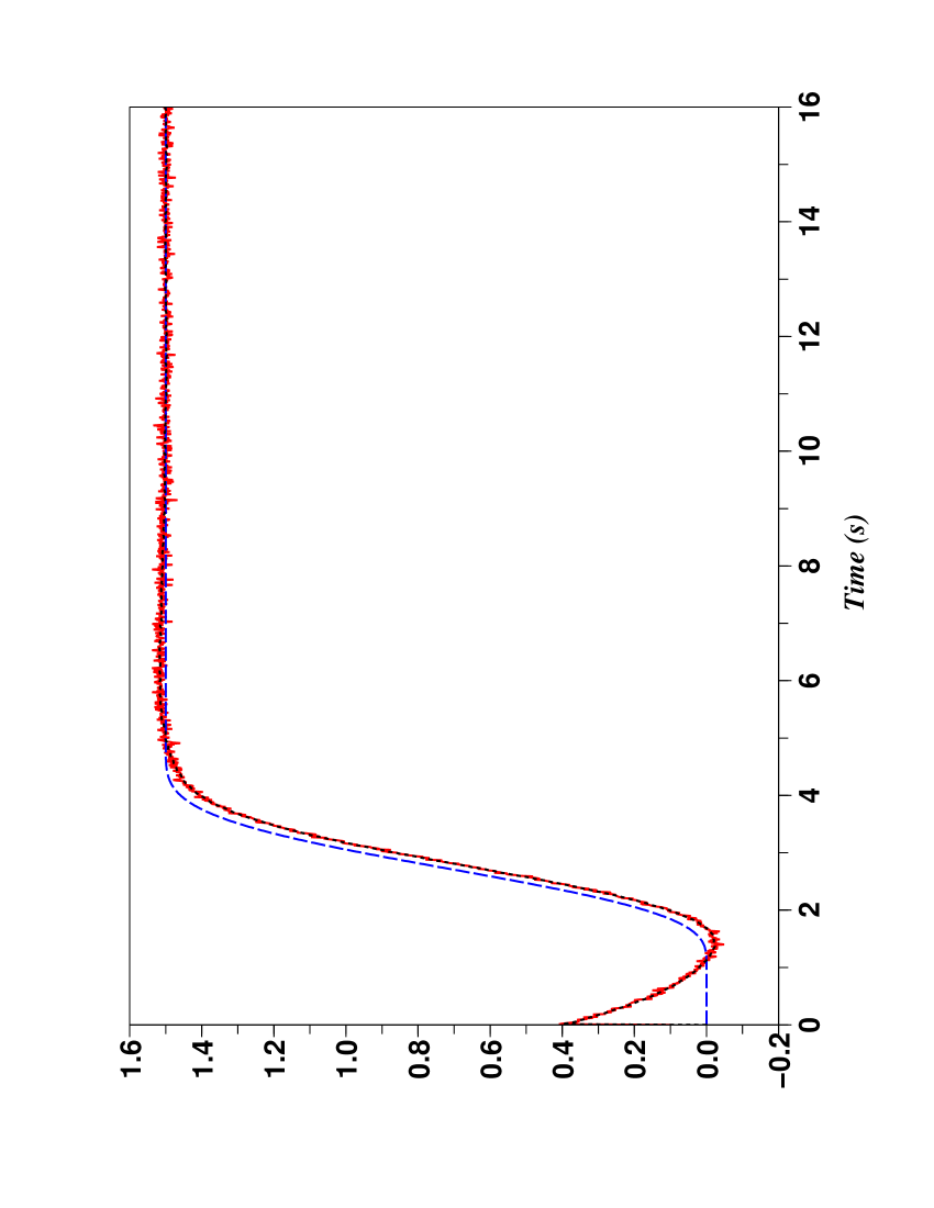
(b) Output (–); reference (- -); denoised output (. .)

(c) PID control

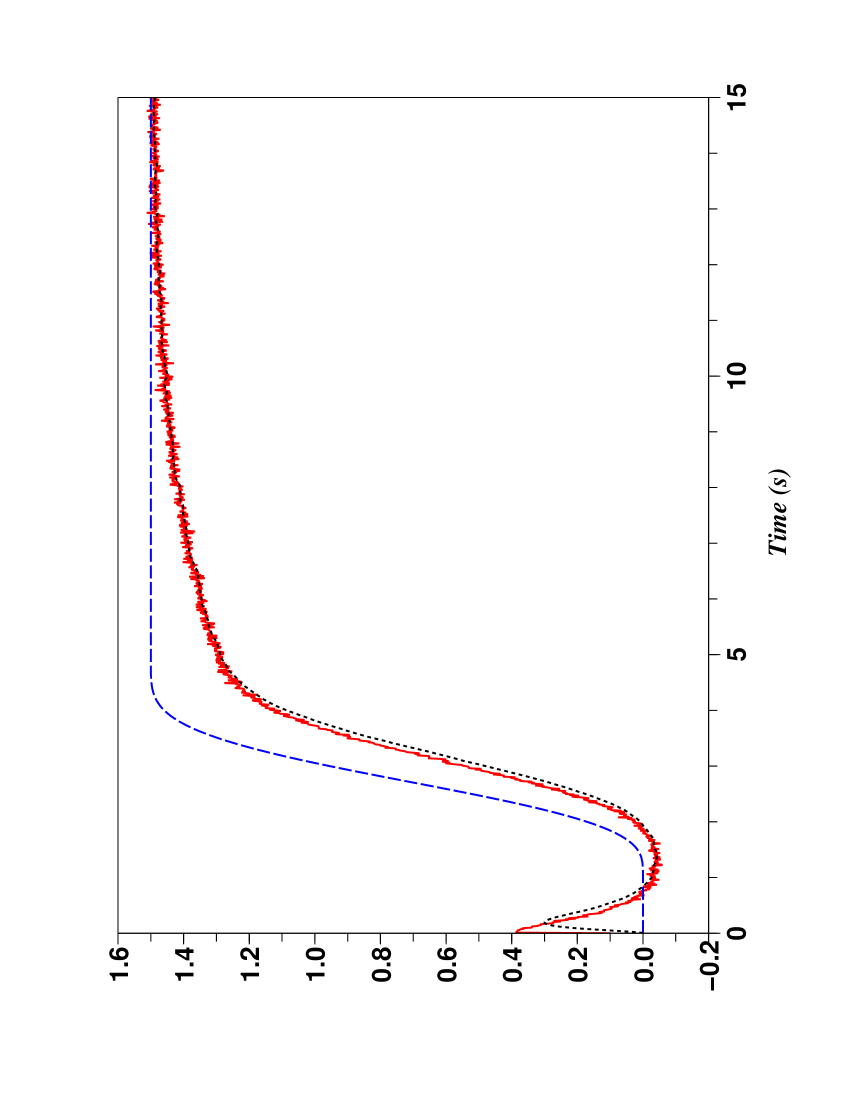
(d) Output (–); reference (- -); denoised output (. .)

Figure 2: Modified stable linear monovariable system

• Fig. 2 indicates a clear cut superiority of our i-PI controller if the ageing process corresponds to a shift of the pole from $1$ to $1.5$, and if the previous graphical identification is not repeated.

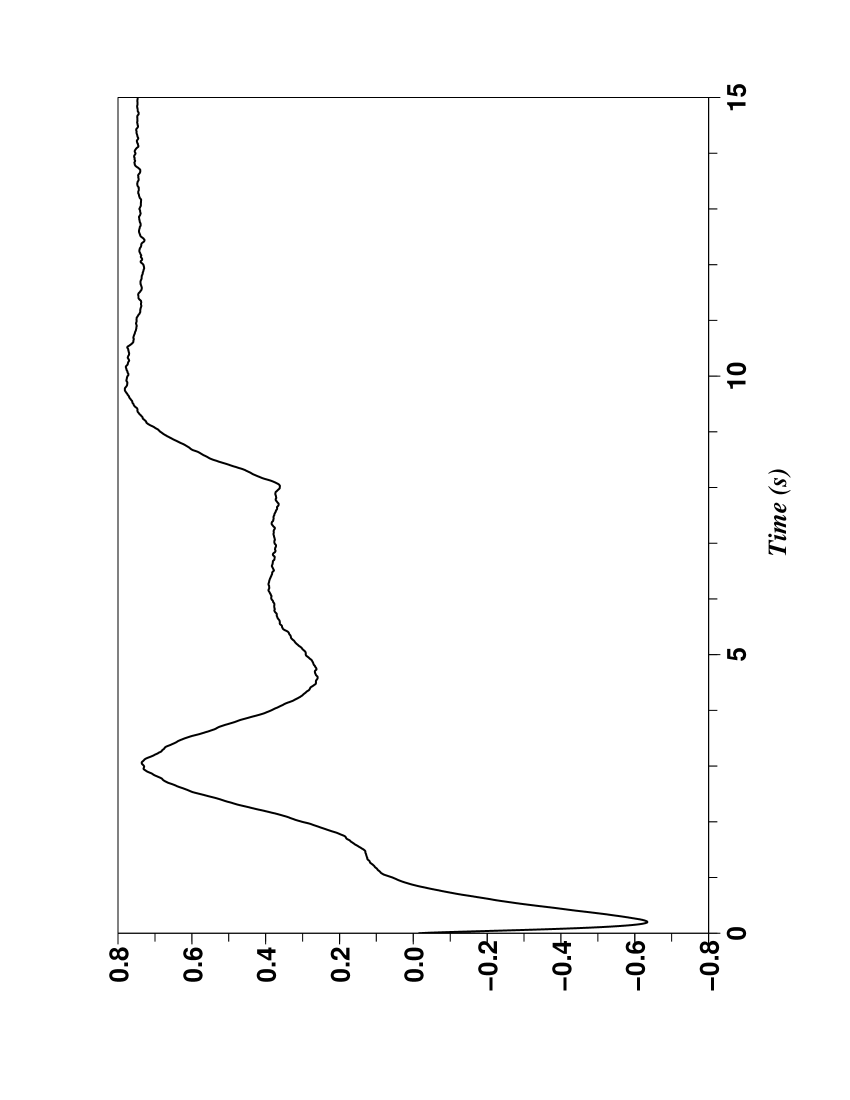
(c) PID control

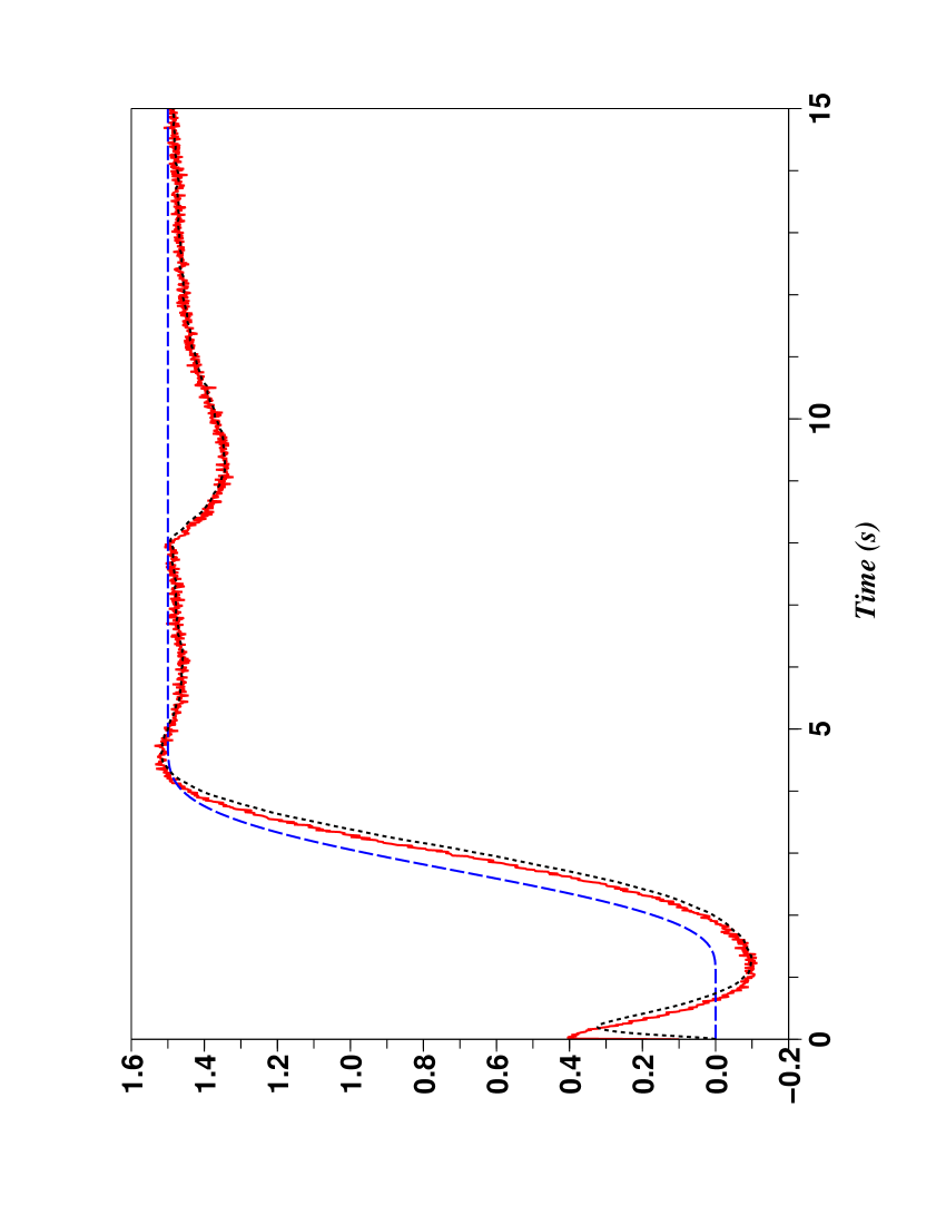
(d) Output (–); reference (- -); denoised output (. .)

Figure 3: Stable linear monovariable system, with an actuator’s fault

• The same conclusion holds, as seen Fig. 3, if there is a $50\%$ power loss of the control.

Remark 8

This example shows that it might useless to introduce delay systems of the type

$$T(s)e^{-Ls},\quad\leavevmode\nobreak\ T\in{\mathbb{R}}(s),\leavevmode\nobreak\ L\geq 0$$ (10)

for tuning classic PID controllers, as often done today in spite of the quite involved identification procedure. It might be reminded that

• the structure and the control of systems of type (10) have been studied in (Fliess, Marquez & Mounier (2002)),

• their identification with techniques stemming also from (Fliess & Sira-Ramírez (2003)) has been studied in (Belkoura, Richard & Fliess (2009); Ollivier, Moutaouakil & Sadik (2007); Rudolph & Woittennek (2007)).

Remark 9

This example demonstrates also that the usual mathematical criteria for robust control become to a large irrelevant. Let us however point out that our control leads always to a pure integrator of order $1$ or $2$, for which the classic frequency techniques (see, e.g., Åström & Murray (2008); Franklin, Powell & Emami-Naeini (2002); Rotella & Zambettakis (2008)) might still be of some interest.

Remark 10

As also shown by this example some fault accommodation may also be achived without having recourse to a general theory of diagnosis.

5.2 A monovariable linear system with a large spectrum

With the system defined by the transfer function

$$\frac{s^{5}}{(s+1)(s+0.1)(s+0.01)(s-0.05)(s-0.5)(s-5)}$$

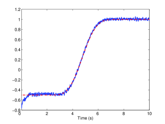
(a) Reference (- -) and output

(b) Control

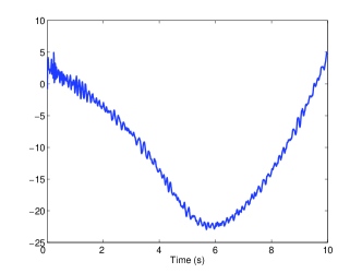
(c) Estimation of $F$

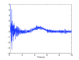
(d) Estimation of $\dot{y}$

Figure 4: Linear monovariable system with a large spectrum

We utilize $\dot{y}=F+u$. A i-PI controller provides the stabilization around a reference trajectory. Fig. 4 exhibits an excellent tracking.

5.3 A multivariable linear system

Introduce the transfer matrix

$$\begin{pmatrix}\frac{s^{3}}{(s+0.01)(s+0.1)(s-1)s}&0\\ \frac{s+1}{(s+0.003)(s-0.03)(s+0.3)(s+3)}&\frac{s^{2}}{(s+0.004)(s+0.04)(s-0.4)(s+4)}\end{pmatrix}$$

For the corresponding system we utilize after a few attempts Eq. (7) with the following decoupled form

$$\dot{y}_{1}=F_{1}+10u_{1}\quad\leavevmode\nobreak\ \ddot{y}_{2}=F_{2}+10u_{2}$$

The stabilization around a reference trajectory $(y_{1}^{\ast},y_{2}^{\ast})$ is ensured by the multivariable i-PID controller

$$\begin{array}[]{l}u_{1}=\frac{1}{10}\left(\dot{y}^{\ast}_{1}-F_{1}+K_{P1}e_{1}+K_{I1}\int e_{1}+K_{D1}\dot{e}_{1}\right)\\ u_{2}=\frac{1}{10}\left(\ddot{y}^{\ast}_{2}-F_{2}+K_{P2}e_{2}+K_{I2}\int e_{2}+K_{D2}\dot{e}_{2}\right)\end{array}$$

where

• $e_{1}=y^{\ast}_{1}-y_{1}$, $e_{2}=y^{\ast}_{2}-y_{2}$;

• $K_{P1}=1$, $K_{I1}=K_{D1}=0$, $K_{P2}=K_{I2}=50$, $K_{D2}=10$.

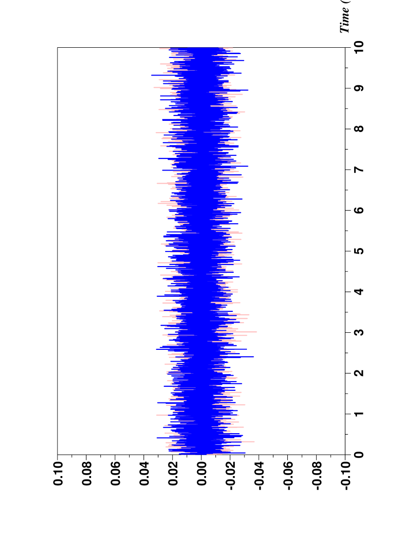
(a) Output’s noises

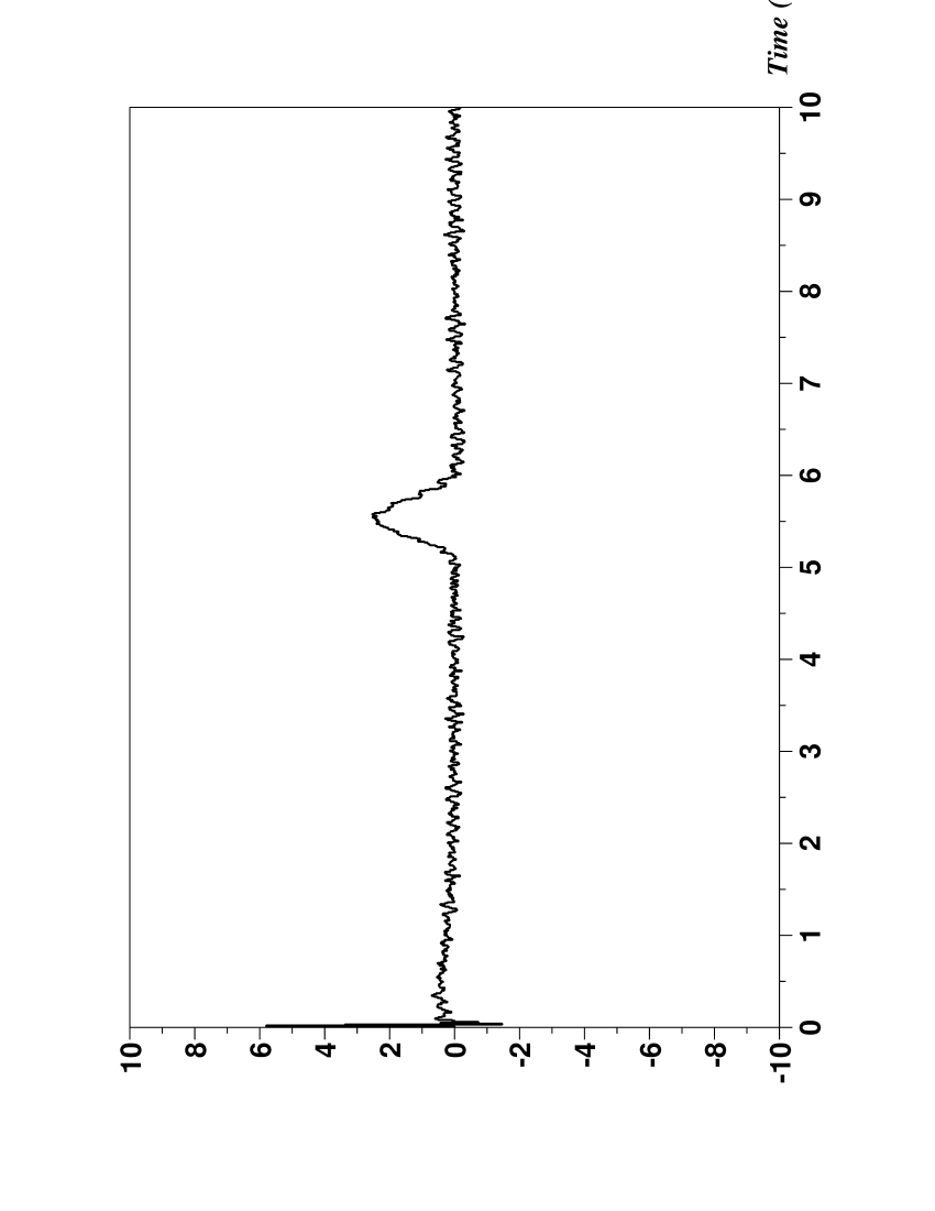
(b) Estimation of $\dot{y}_{1}$

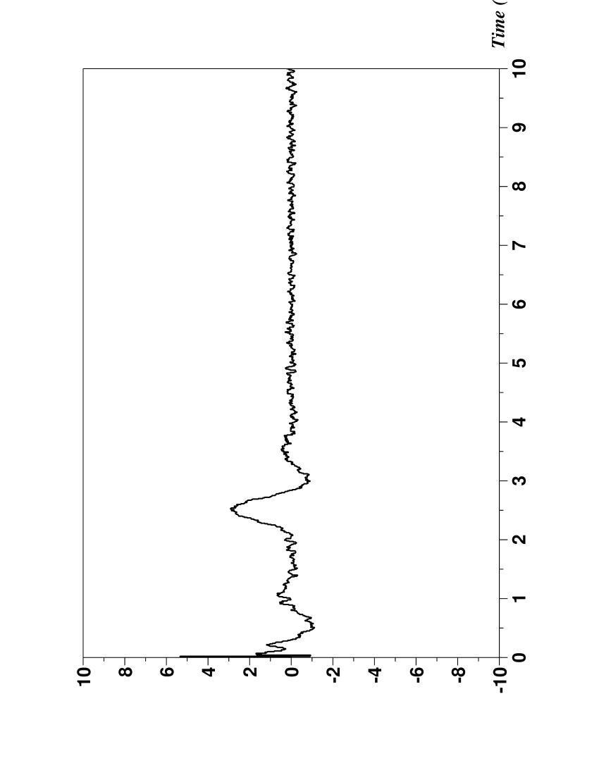
(c) Estimation of $\dot{y}_{2}$

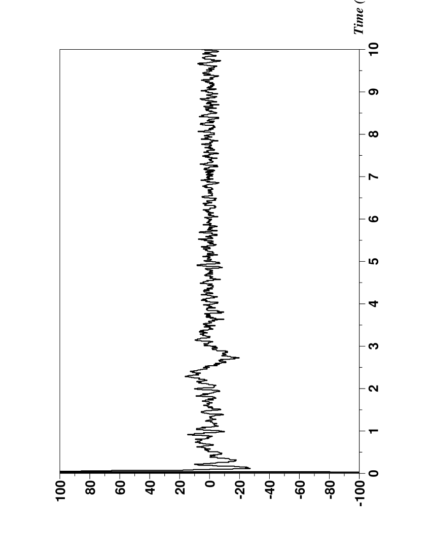
(d) Estimation of $\ddot{y}_{2}$

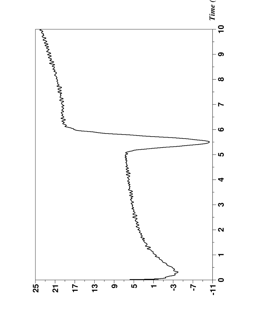
(e) Estimation of $F_{1}$

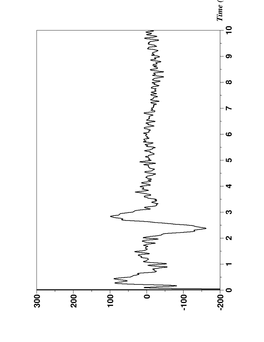
(f) Estimation of $F_{2}$

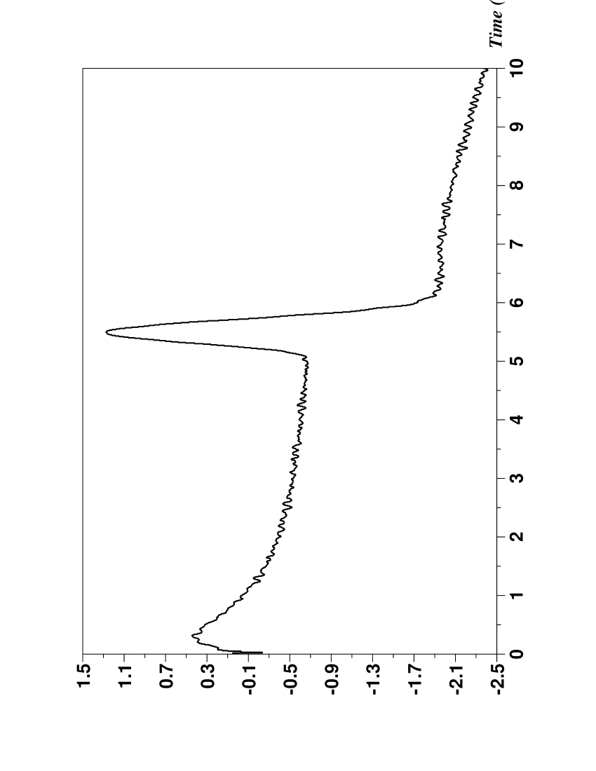
(g) Control $u_{1}$

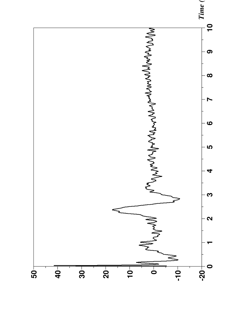
(h) Control $u_{2}$

Figure 5: Linear multivariable system

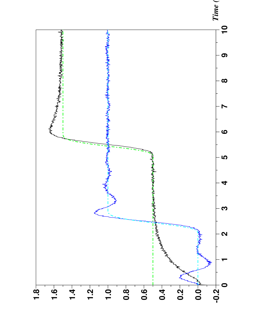
(a) i-PID: references (- -) and outputs

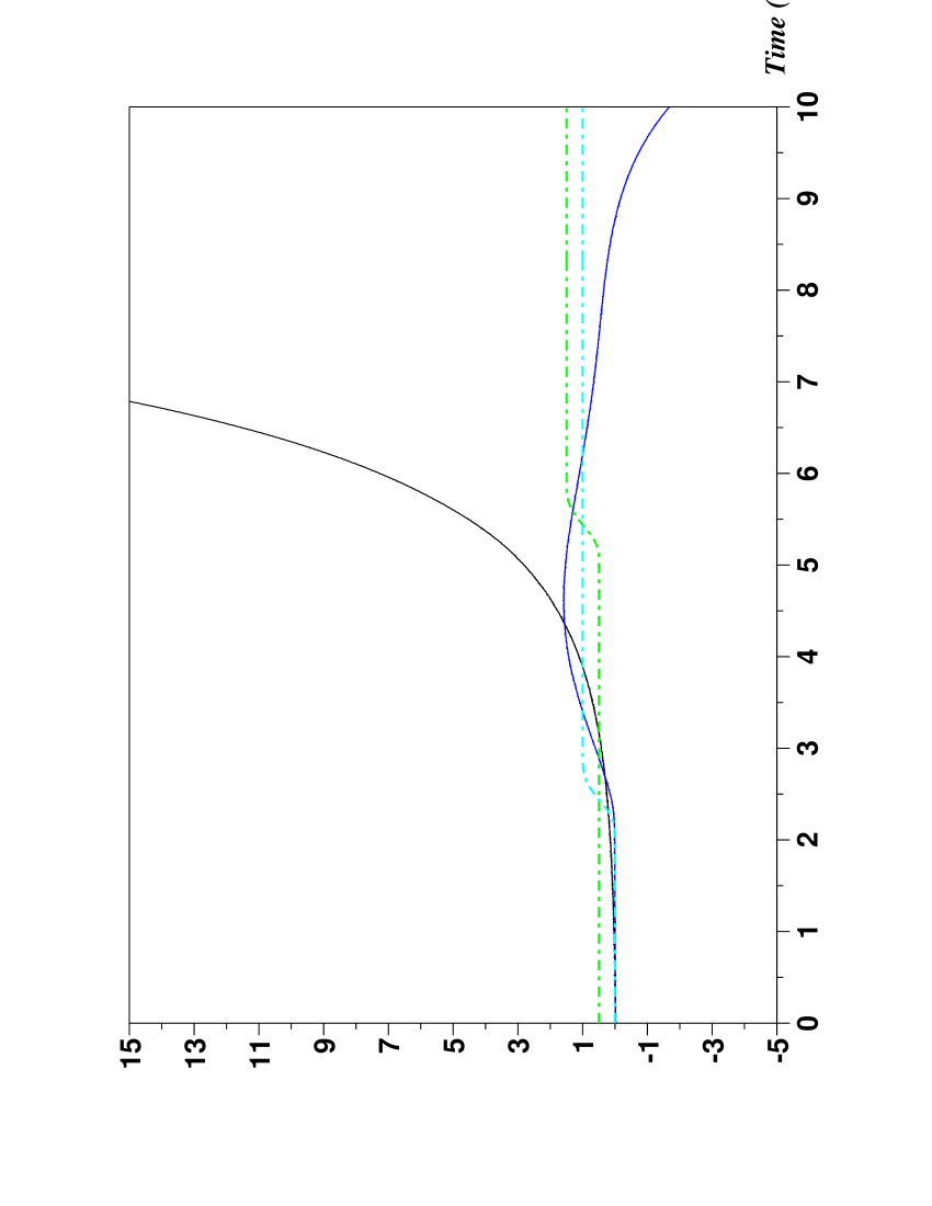
(b) PID: references (- -) and outputs

Figure 6: Linear multivariable system

The performances displayed on Fig. 5 and 6 are excellent. Fig. 6-(b) shows the result if we would set $F_{1}=F_{2}=0$: it should be compared with Fig. 6-(a).

Remark 11

Model reduction is often utilized for the kind of systems studied in Sect. 5.2 and Sect. 5.3 (see, e.g., Antoulas (2005); Obinata & Anderson (2001)).

5.4 An unstable monovariable nonlinear system

5.4.1 i-PID

For $\dot{y}-y=u^{3}$ we utilize for Eq. (2) the local model $\dot{y}=F+u$. The stabilization around a reference trajectory $y^{\ast}$ is provided by the i-PI controller

$$u=-F+\dot{y}^{\star}+K_{P}e+K_{I}\int e$$ (11)

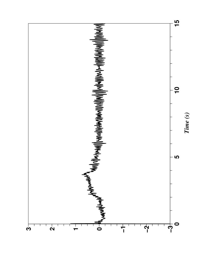
(a) Estimation of $\dot{y}$

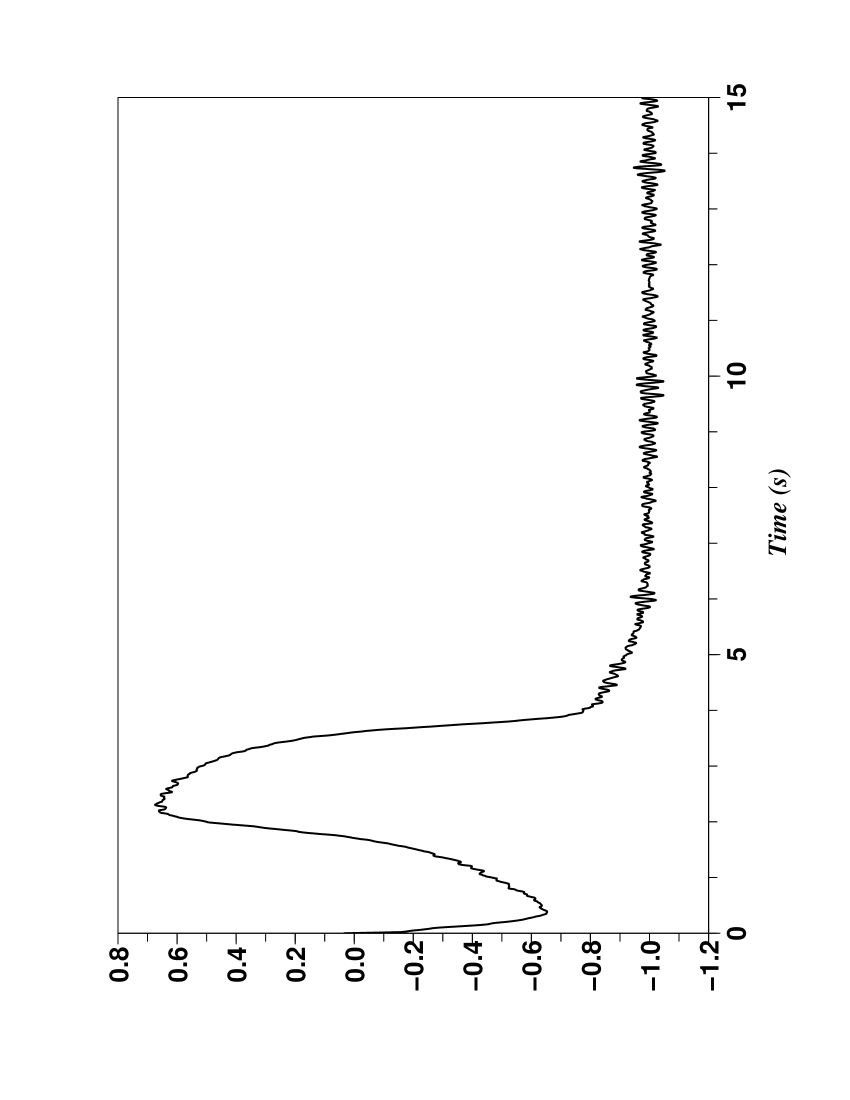
(b) Commande

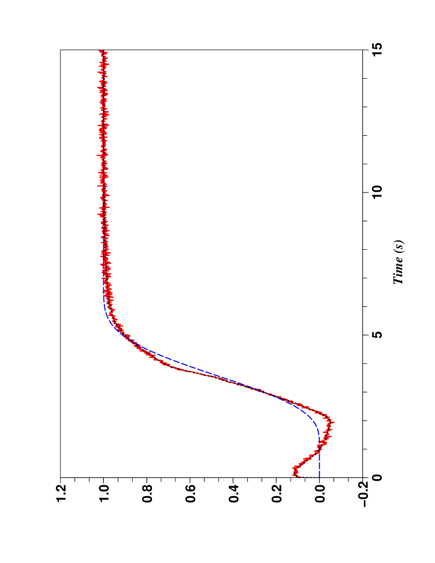
(c) Output (–); reference (- -); denoised output (. .)

Figure 7: Instable nonlinear monovariable system

where $K_{P}=-2$, $K_{I}=-1$. The simulations displayed in Fig. 7 are excellent.

5.4.2 Anti-windup

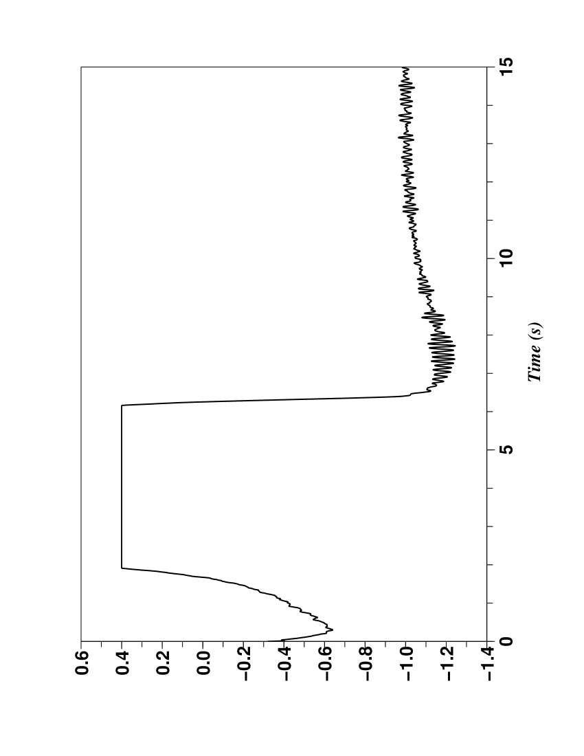
(a) Commande

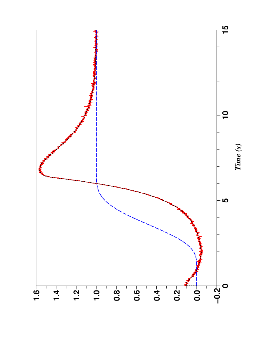
(b) Output (–); reference (- -); denoised output (. .)

Figure 8: Instable nonlinear system: saturated control without anti-windup

We now assume that $u$ should satisfy the following constraints $-2\leq u\leq 0.4$. The performances displayed by Fig. 8 are mediocre if an anti-windup is not added to the classic part of the i-PI controller. Our solution is elementary: as soon as the control variable gets saturated, the integral $\int e$ in Eq. (11) is maintained constant.

5.5 Ball and beam

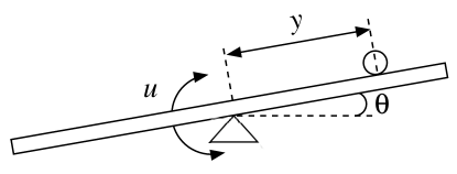
Figure 10: The ball and beam example

Fig. 10 displays the famous ball and beam example, which obeys to the equation $\ddot{y}=By\dot{u}^{2}-BG\sin u$, where $u=\theta$ is the control variable. This monovariable system, which is not linearizable by a static state feedback, is therefore not flat. It is thus difficult to handle.

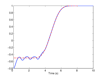
(a) Reference (- -) and output

(b) Control

(c) Estimation of $F$

(d) Reference (- -); output in the noisy case

Figure 11: Polynomial trajectory for the ball and beam

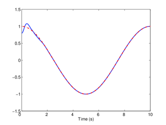
(a) Reference (- -); output

(b) Control

(c) Estimation of $F$

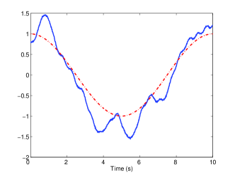
(d) Reference (- -); output in the noisy case

Figure 12: Sinusoidal trajectory for the ball and beam

We have chosen for Eq. (2) $\ddot{y}=F+100u$. In order to satisfy as well as possible the experimental conditions, the control variable is saturated: $-\pi/3<u<\pi/3$ and $-\pi<\dot{u}<\pi$. Fig. 11 and Fig. 12 display two types of trajectories: a Bézier polynomial and a sine function. We obtain in both cases excellent trackings thanks to an i-PID controller. In the Figures 11-(b), 12-(b), 11-(c), 12-(c) the control variable and the estimations of $F$ are presented in the noiseless case. Compare with the Figures 11-(d) and 12-(d)) where a corrupting noise is added.

5.6 The three tank example

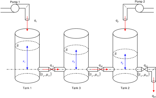
Figure 13: The 3 tank system

The three tank example in Fig. 13 is quite popular in diagnosis. It obeys to the equations:

$$\begin{cases}\begin{array}[]{ll}\dot{x}_{1}=&-C_{1}\text{sign}(x_{1}-x_{3})\sqrt{|x_{1}-x_{3}|}+u_{1}/S\\ \dot{x}_{2}=&C_{3}\text{sign}(x_{3}-x_{2})\sqrt{|x_{3}-x_{2}|}\\ &-C_{2}\text{sign}(x_{2})\sqrt{|x_{2}|}+u_{2}/S\\ \dot{x}_{3}=&C_{1}\text{sign}(x_{1}-x_{3})\sqrt{|x_{1}-x_{3}|}\\ &-C_{3}\text{sign}(x_{3}-x_{2})\sqrt{|x_{3}-x_{2}|}\\ y_{1}=&x_{1}\\ y_{2}=&x_{2}\\ y_{3}=&x_{3}\\ \end{array}\end{cases}$$

where

$$\begin{array}[]{l}C_{n}=(1/S).\mu_{n}.S_{p}\sqrt{2g},n=1,2,3;\\ S=0.0154\leavevmode\nobreak\ m\leavevmode\nobreak\ \text{(tank section)};\\ Sp=5.10^{-5}\leavevmode\nobreak\ m\leavevmode\nobreak\ \text{(pipe section between the tanks)};\\ g=9.81\leavevmode\nobreak\ m.s^{-2}\leavevmode\nobreak\ \text{(gravity)};\\ \mu_{1}=\mu_{3}=0.5\text{,}\leavevmode\nobreak\ \mu_{2}=0.675\leavevmode\nobreak\ \text{(viscosity coefficients)}.\end{array}$$

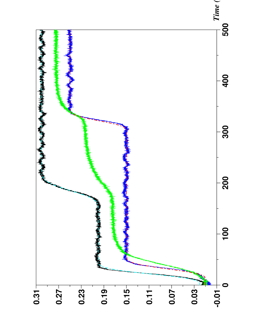
(a) References (- -); outputs

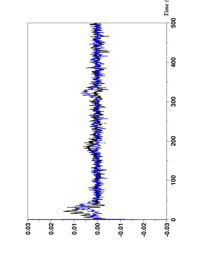
(b) Estimation of the derivatives $\dot{y}_{1}$ (-) and $\dot{y}_{2}$ (- -), which is shifted back $0.02$

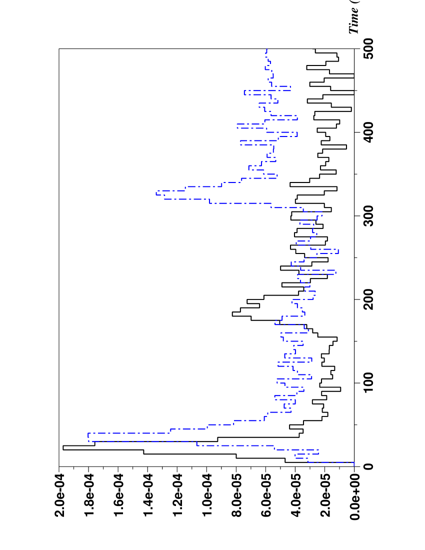
(c) Control $u_{1}$ (-) and $u_{2}$ (- -)

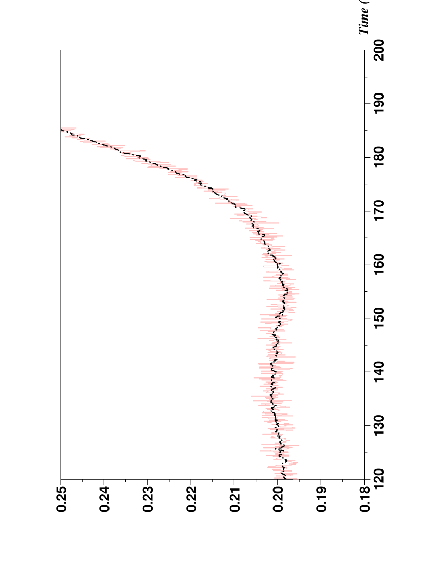
(d) Denoising

Figure 14: Simulations for the 3 tank system

As often in industry we utilize a zero-hold control (see Fig. 14- (c)). A decoupled Eq. (7) is employed here as we already did in Sect. 5.3: $\dot{y}_{i}=F_{i}+200u_{i}$, $i=1,2$. Fig. 14-(a) displays the trajectories tracking. The derivatives estimation in Fig. 14-(b) is excellent in spite of the additive corrupting noise. The nominal controls (Fig. 14-(c)) are not very far from those we would have computed with a flatness-based viewpoint (see Fliess, Join & Sira-Ramírez (2005)). We also utilize the following i-PI controllers

$$u_{i}=\frac{1}{200}\left(\dot{y}_{i}^{\ast}-F_{i}+10e_{i}+2.10^{-2}\int e_{i}\right)\quad i=1,2$$

where $y_{i}^{\ast}$ is the reference trajectory, $e_{i}=y_{i}^{\ast}-y_{i}$. In order to get a good estimate of $e_{i}$ we are denoising $y_{i}$ (see Fig. 14-(d)) according to the techniques of Sect. 3.

6 Control with a restricted model

6.1 General principles

6.1.1 Flatness

The system (4) is assumed to be square, i.e., $m=p$, and flat. Moreover ${\boldsymbol{y}}=(y_{1},\dots,y_{m})$ is assumed to be a flat output, ı.e., $\bar{M}_{j}=0$, $j=1,\dots,m$. It yields locally

$$u_{j}=\Psi_{j}({\boldsymbol{y}},\dots,{\boldsymbol{y}}^{(\bar{N}_{j})}),\quad\leavevmode\nobreak\ j=1,\dots,m$$ (12)

Flatness-based control permits to select easily an efficient reference trajectory ${\boldsymbol{y}}^{\star}$ to which corresponds via Eq. (4) and Eq. (12) the open loop control ${\boldsymbol{u}}^{\star}$. Let ${\boldsymbol{e}}={\boldsymbol{y}}-{\boldsymbol{y}}^{\star}$ be the tracking error. We assume the existence of a feedback controller ${\boldsymbol{u}}_{\mbox{\rm feedback}}({\boldsymbol{e}})$ such that

$${\boldsymbol{u}}={\boldsymbol{u}}^{\star}+{\boldsymbol{u}}_{\mbox{\rm feedback}}({\boldsymbol{e}})$$ (13)

ensures a stable tracking around the reference trajectory.

6.1.2 Intelligent controllers

Replace Eq. (4) by

$$\Phi_{j}({\boldsymbol{y}},\dots,{\boldsymbol{y}}^{(\bar{N}_{j})},{\boldsymbol{u}},\dots,{\boldsymbol{u}}^{(\bar{M}_{j})})+G_{j}=0$$ (14)

where the $G_{j}$, $j=1,\dots,m$, stand for the unmodeled parts. Eq. (12) becomes then

$$u_{j}=\Psi_{j}({\boldsymbol{y}},\dots,{\boldsymbol{y}}^{(\bar{N}_{j})})+H_{j},\quad\leavevmode\nobreak\ j=1,\dots,m$$ (15)

where $H_{j}\neq G_{j}$ in general. Thanks to Eq. (15), $H_{j}$ is estimated in the same way as the fault variables and the unknown perturbations are in (Fliess, Join & Sira-Ramírez (2008)). Consider again ${\boldsymbol{y}}^{\star}$ and ${\boldsymbol{u}}^{\star}$ as they are defined above. The intelligent controller, or i-controller, follows from Eq. (13)

$${\boldsymbol{u}}={\boldsymbol{u}}^{\star}+\left(\begin{array}[]{c}H_{1}\\ \vdots\\ H_{m}\end{array}\right)+{\boldsymbol{u}}_{\mbox{\rm feedback}}({\boldsymbol{e}})$$

It ensures tracking stabilization around the reference trajectory.

6.2 Frictions and nonlinearities

A point mass $m$ at the end of a spring of length $y$ obeys to the equation

$$m\ddot{y}=-{\mathcal{K}}(y)+{\mathcal{F}}(\dot{y})-d\dot{y}+F_{\tiny{\mbox{\rm ext}}}$$ (16)

where

• $F_{\tiny{\mbox{\rm ext}}}=u$ is the control variable;

• $d$ and ${\mathcal{F}}(\dot{y})$ are due to complex friction phenomena;

• ${\mathcal{K}}(y)=k_{1}y+k_{3}y^{3}$ exhibits a cubic nonlinearity of Duffing type;

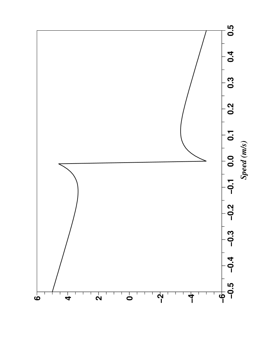
(a) The friction law

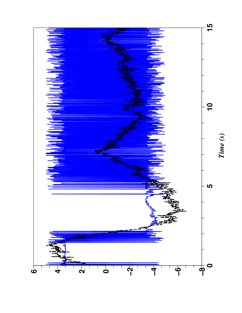
(b) Friction ${\mathcal{F}}(\dot{y})$ (–); Estimation of the whole unknown effects $[{\mathcal{G}}(\dot{y})]_{e}$ (- -)

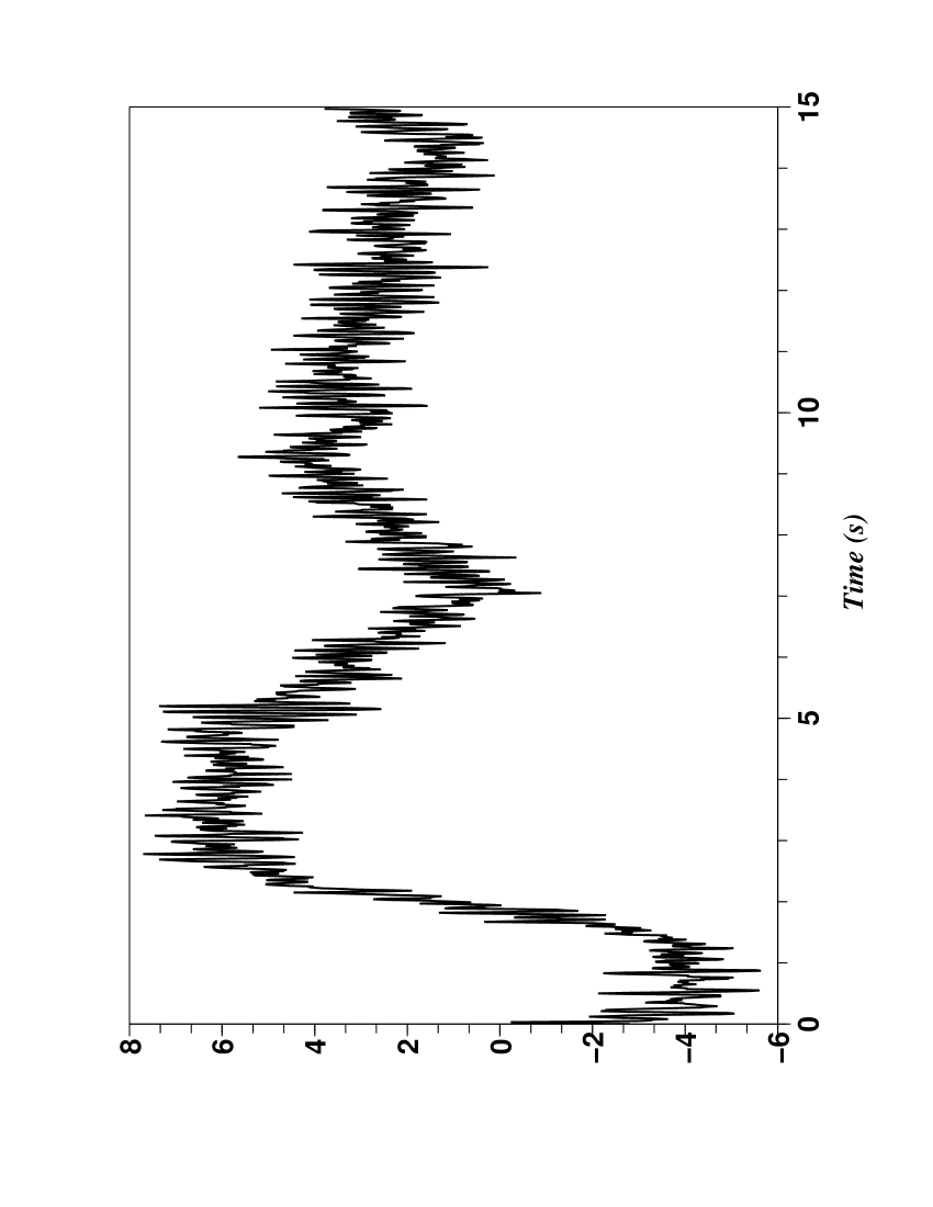
(c) i-PID control

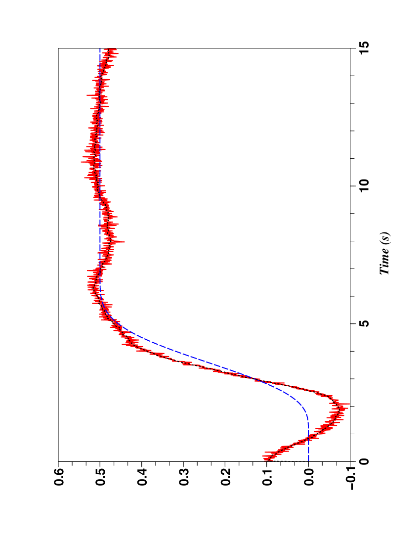
(d) i-PID: output (–), reference (- -); denoised output (. .)

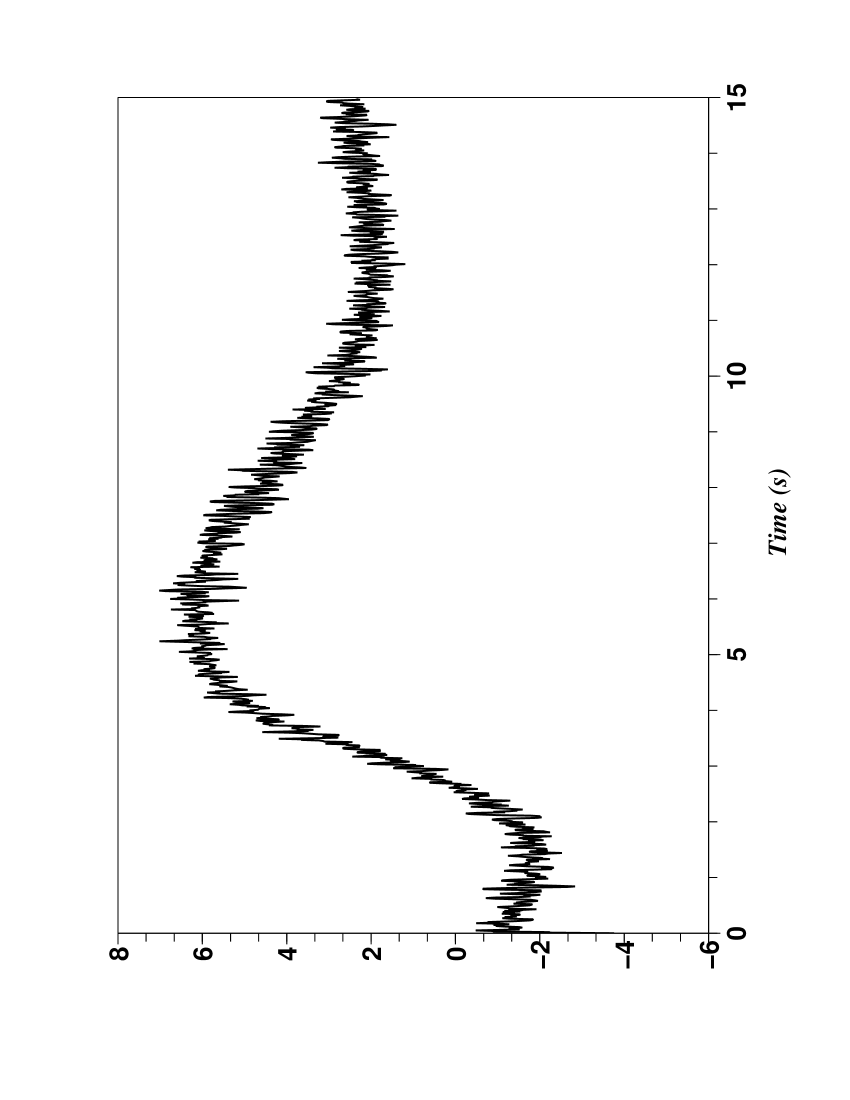
(e) Flatness-based control + classic PID

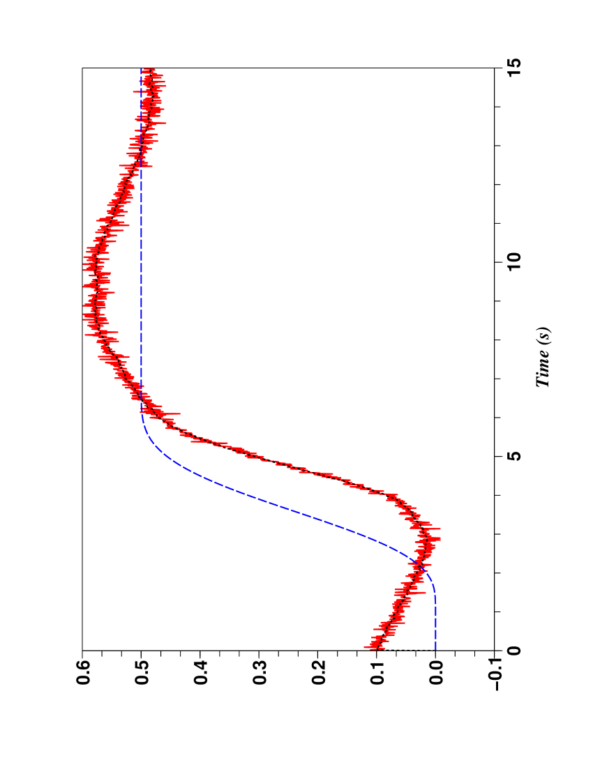
(f) Flatness-based control + classic PID: output (–), reference (- -), denoised output (. .)

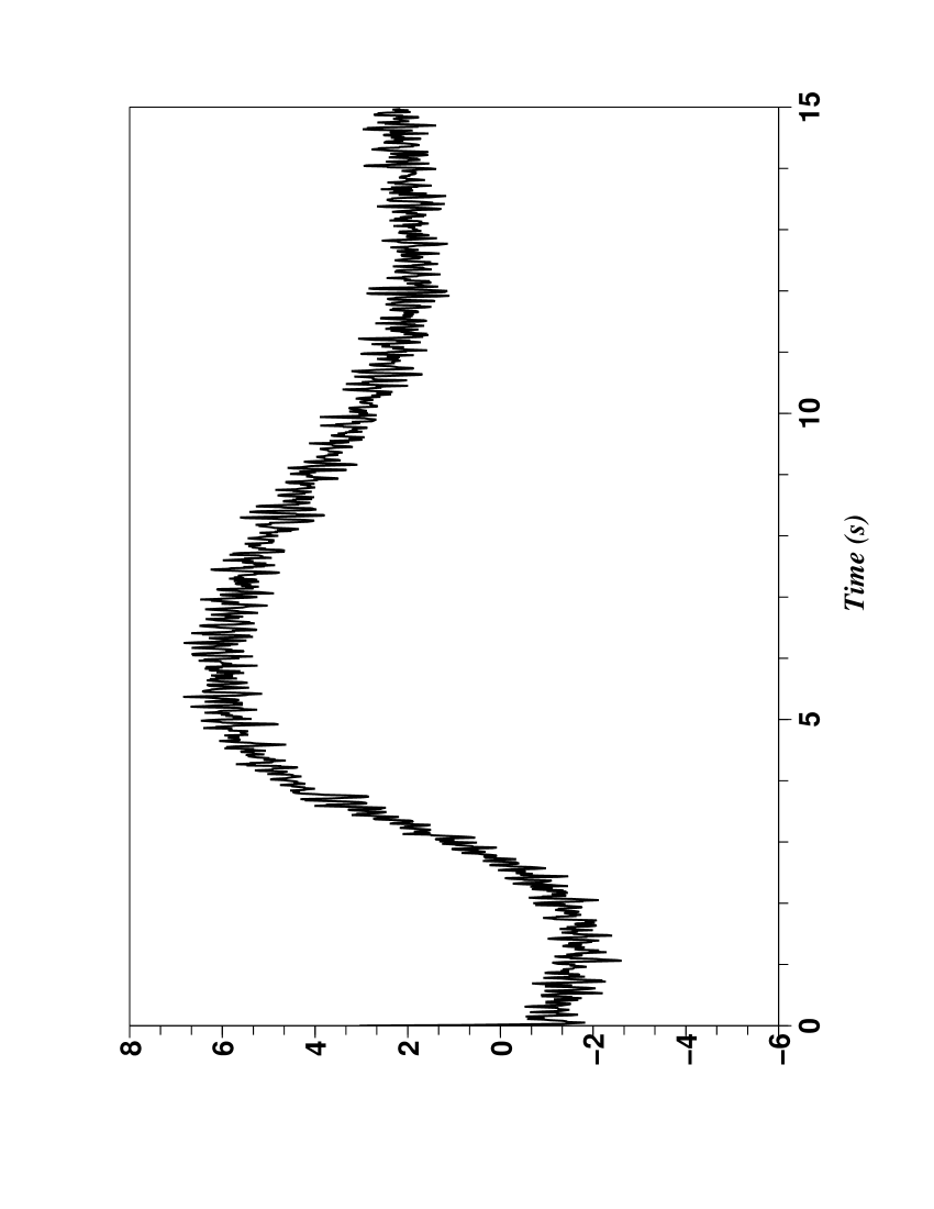
(g) Non-flatness-based control + PID

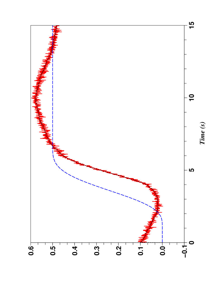
(h) Non-flatness-based control: output (–), reference (- -), denoised output (. .)

Figure 15: The spring with unknown with nonlinearity, friction and damping

The mass $m=0.5$ is known; there is a possible error of $33\%$ for $k_{1}=3$ and we utilize $\hat{k}_{1}=2$; $d$ and $k_{3}$, which are unknown, are equal to $5$ and $10$ in the numerical simulations. For the frictions, we have chosen for the sake of computer simulations the well known model due to Tustin (1947). Fig. 15-(a) exhibits its quite wild behavior when the sign of the speed is changing.

6.2.1 A classic PID controller

The PID controller is tuned only thanks to the restricted model $m\ddot{y}=-\hat{k}_{1}y+u$. Its gains are determined in such a way that all the poles of the closed-loop system are equal to $-3$: $K_{P}=-\hat{k}_{1}+27m$, $K_{I}=-27m$, $K_{D}=9m$.

6.2.2 The corresponding i-PID controller

Pick up a reference trajectory $y^{\star}$. Set

$$u^{\star}=m\ddot{y}^{\star}+\hat{k}_{1}y^{\star}$$

Our i-PID controller is given by

$$F_{\tiny{\mbox{\rm ext}}}=u=u^{\star}-[{\mathcal{G}}]_{e}+\mbox{\rm PID}(e)$$ (17)

where

• ${\mathcal{G}}={\mathcal{F}}(\dot{y})-(k_{1}-\hat{k}_{1})y-k_{3}y^{3}-d\dot{y}$, which stands for the whole set of unknown effects, is estimated via

  $$[{\mathcal{G}}]_{e}=m[\ddot{y}]_{e}+\hat{k}[y]_{e}-F_{\tiny{\mbox{\rm ext}}}$$

  which follows from Eq. (16) ($[y]_{e}$ and $[\ddot{y}]_{e}$ are the denoised output variable and its denoised $2^{nd}$-order derivative – see Fig. 15-(d,f));

• $\mbox{\rm PID}(e)$, $e=y-y^{\star}$, is the above classic PID controller.

6.2.3 Numerical simulations

The performances of our i-PID controller (17), which are displayed in Fig. 15-(c,d), are excellent. When compared to the Figures

• 15-(e,f), where

  • flatness-based control is employed for determined the open-loop output and input variables,

  • the loop is closed via a classic PID controller, which does not take into account the unknown effects;

• 15-(g,h), where only a classic PID controller is used, without any flatness-based control;

the superiority of our control design is obvious. This superiority is increasing with the friction.

6.3 Non-minimum phase systems

Consider the transfer function

$$\frac{s-a}{s^{2}-(b+c)s+bc}$$

$a,b,c\in\mathbb{R}$ are respectively its zero and its two poles. The corresponding input-output system is non-minimum phase if $a>0$. The controllable and observable state-variable representation

$$\begin{cases}\dot{x}_{1}=x_{2}\\ \dot{x}_{2}=(b+c)x_{2}-bcx_{1}+u\\ y=x_{2}-ax_{1}\end{cases}$$ (18)

shows that $z=x_{1}$ is a flat output. The flat output is therefore not the measured output, as we assumed in Sect. 6.1.1. Our control design has therefore to be modified.

6.3.1 Control of the exact model

To a nominal flat output $z^{\star}$ corresponds a nominal control variable

$$u^{\star}=\ddot{z}^{\star}-(b+c)\dot{z}^{\star}+bcz^{\star}$$

and a nominal output variable

$$y^{\star}=\dot{z}^{\star}-az^{\star}$$ (19)

Introduce the GPI controller (Fliess, Marquez, Delaleau & Sira-Ramírez (2002))

$$\begin{array}[]{lc}u=&u^{\star}+\gamma\int(u-u^{\star})+K_{P}(y-y^{\star})\\ &+K_{I}\int(y-y^{\star})+K_{II}\int\!\!\int(y-y^{\star})\end{array}$$ (20)

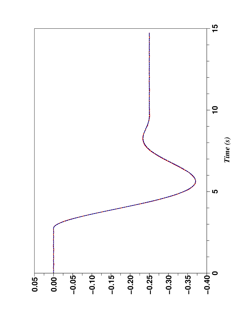
(a) $u$ (–); $u^{\star}$ (- -)

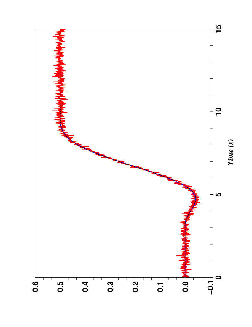
(b) Output (–); reference (- -); denoised output (. .)

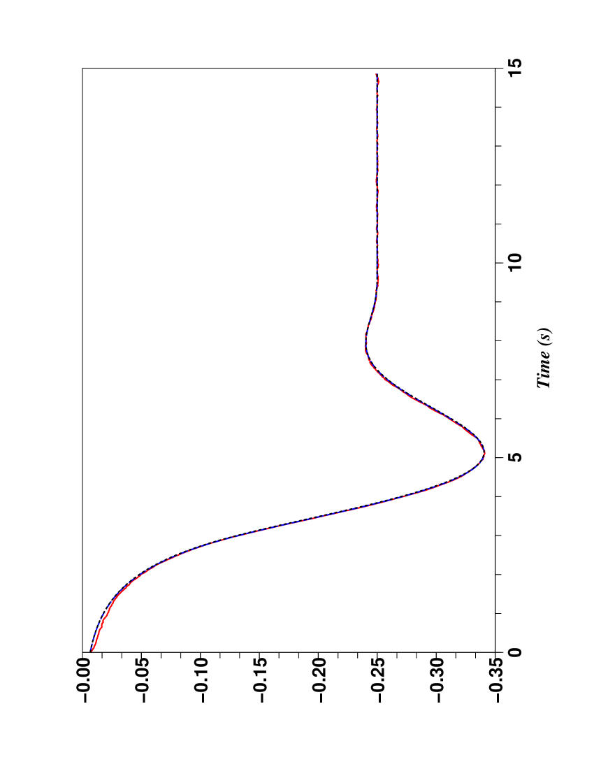
(c) $u$ (–); $u^{\star}$ (- -)

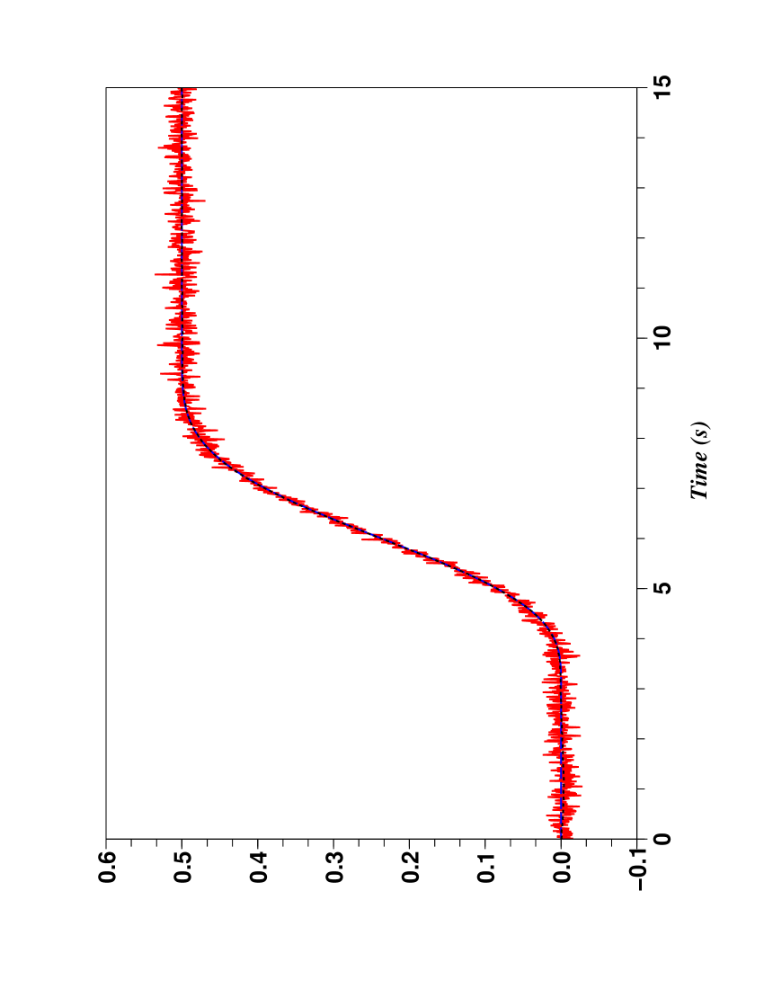
(d) Output (–); reference (- -); denoised output (. .)

Figure 16: Non-minimum phase system

where the coefficients $\gamma,K_{P},K_{I},K_{II}\in\mathbb{R}$ are chosen in order to stabilize the error dynamics $e=z-z^{\star}$. Excellent performances are displayed in Figures 16-(a) and (b), where $a=1$, $b=-1$, $c=-0.5$, even with an additive corrupting noise. See Figures 16-(c) and (d) for $y^{\star}$ and $z^{\star}$ which is calculated by integrating Eq. (19) back in time.

6.3.2 Unmodeled effects

The second line of Eq. (18) may be written again as

$$\dot{x}_{2}=(b+c)x_{2}-bcx_{1}+u+\varpi$$

where $\varpi$ stands for the unmodeled effects, like frictions or an actuator’s fault. Replace the nominal control variable $u^{\star}$ of Sect. 6.3.1 by

$$u_{\tiny{\mbox{\rm pert}}}^{\star}=u^{\star}-[\varpi]_{e}$$

where $[\varpi]_{e}$ is the estimated value of $\varpi$, which is given by

$$[\varpi]_{e}=-\left(\frac{[\ddot{y}]_{e}-(b+c)[\dot{y}]_{e}+bc[y]_{e}-[\dot{u}]_{e}}{a}+u\right)$$

Moreover,

$$\begin{array}[]{lc}{[\dot{u}]_{e}}=&\dot{u}^{\star}+\gamma(u-u^{\star})+K_{P}([\dot{y}]_{e}-\dot{y}^{\star})\\ &+K_{I}([y]_{e}-y^{\star})+K_{II}\int([y]_{e}-y^{\star})\end{array}$$

follows from Eq. (20).

Start with the Figures 17 and 18, where $\varpi=-0.5$, $a=1$, $b=-1$, $c=-0.5$. Fig. 17-(b), where the nominal control is left unmodified, and Fig. 17-(e), where it is modified, demonstrate a clear-cut superiority of our approach, even with an additive corrupting noise.

In Fig. 19, $\varpi$ is no more assumed to be constant, but equal to $-0.1\dot{y}$. In the numerical simulations, $a=2$, $b=-1$ $c=1$. If $\varpi$ is not estimated, it influences the tracking quite a lot even if its amplitude is weak. When $\varpi$ is estimated on the other hand, the results are excellent, even with an additive corrupting noise.

7 Conclusion

The results which were already obtained with our intelligent PID controllers lead us to the hope that they will greatly improve the practical applicability and the performances of the classic PIDs, at least for all finite-dimensional systems which are known to be non-minimum phase within their operating range:

• the tuning of the gains of i-PIDs is straightforward since

  • the unknown part is eliminated,

  • the control design boils down to a pure integrator of order $1$ or $2$;

• the identification techniques for implementing classic PID regulators, which are often imprecise and difficult to handle, are becoming obsolete.

Model-free control and the control with a restricted model seem to question the very principles of modeling in applied sciences, at least when one wishes to control some concrete plant. This might be a fundamental “epistemological” change, which needs of course to be further discussed and analyzed. A natural extension to uncontrolled systems is being developed via various questions in financial engineering: see already the preliminary studies in (Fliess & Join (2008b, 2009a, 2009b)).

(a) i-PI control

(b) Output (–); reference (- -); denoised output (. .)

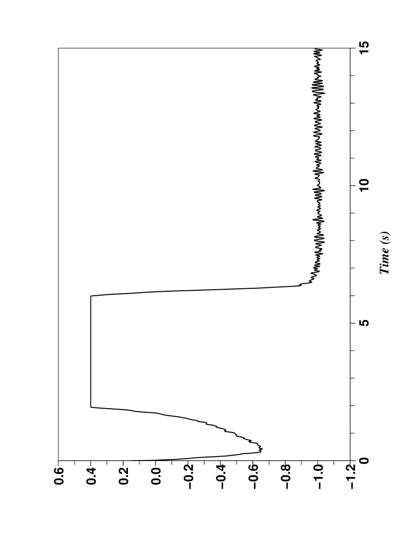
(a) Commande

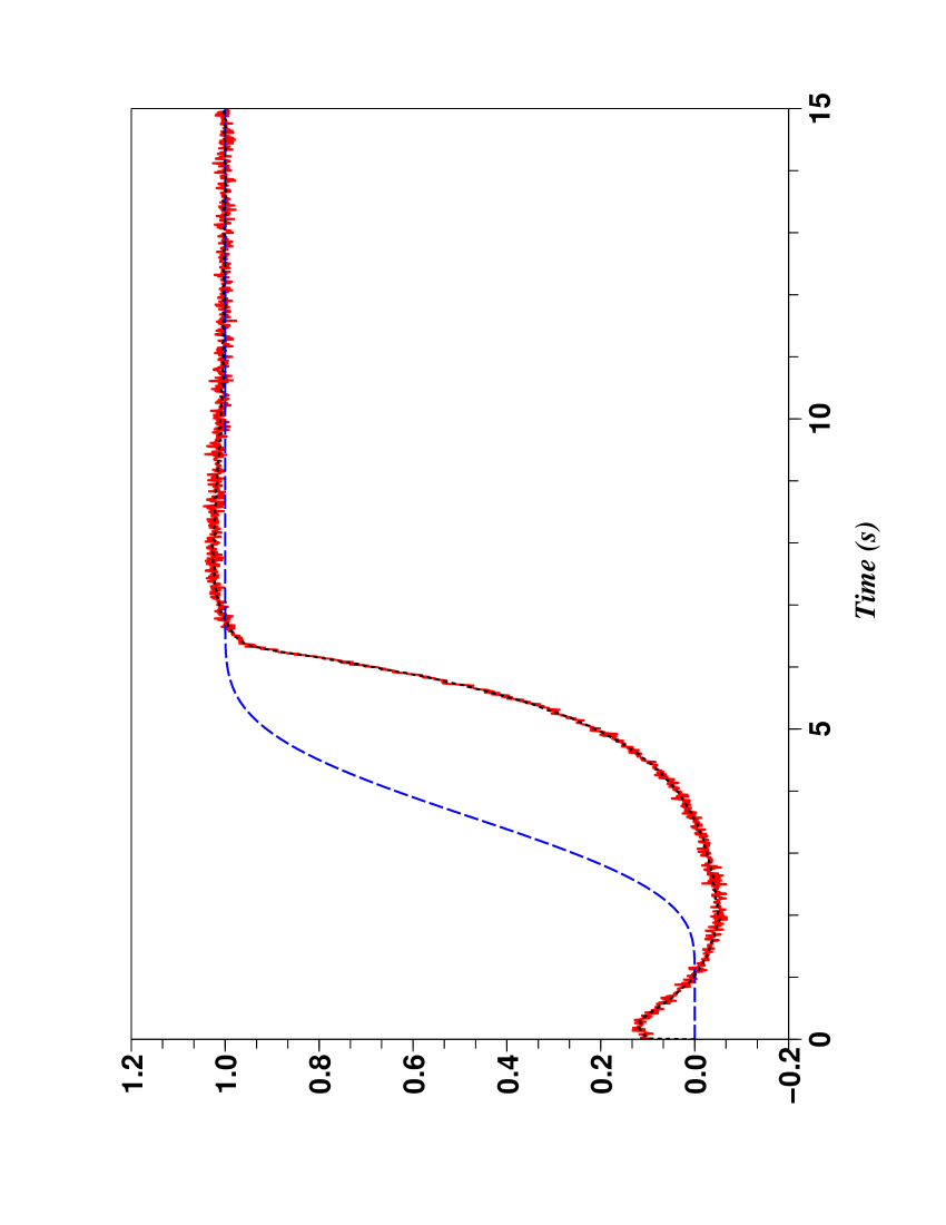
(b) Output (–); reference (- -); denoised output (. .)

Figure 9: Instable nonlinear system: saturated control with anti-windup

(a) $u$ (–); $u^{\star}$ (- -)

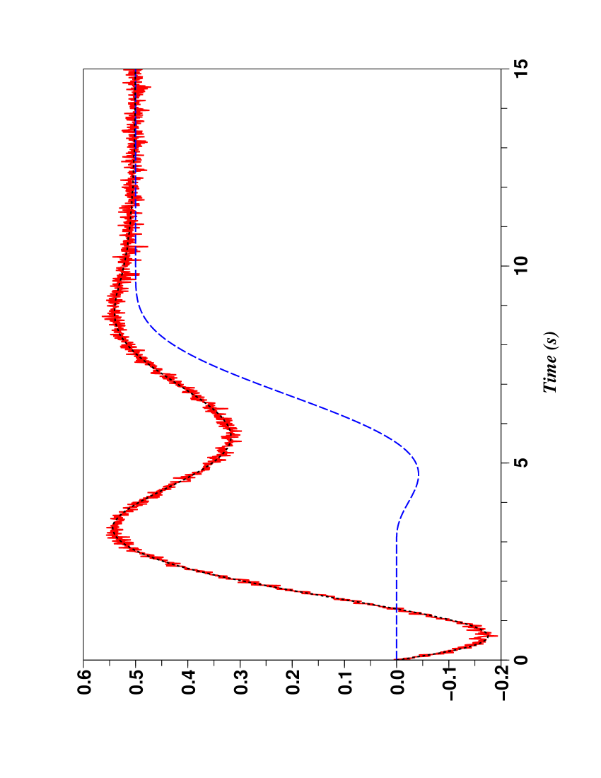
(b) Output (–); reference (- -); denoised output (. .)

(c) Perturbation (- -); estimated perturbation (–)

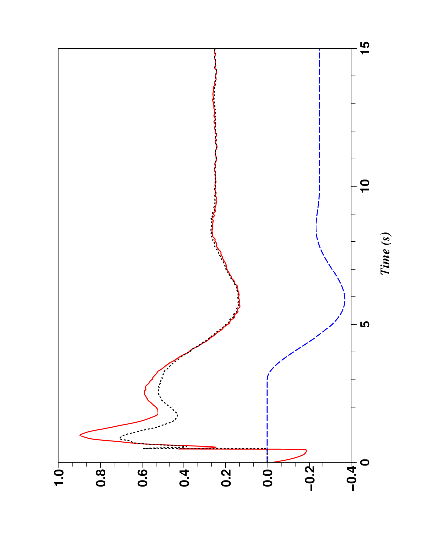
(d) $u$ (–); $u^{\star}$ (- -); $u^{\star}_{\text{pert}}$(. .)

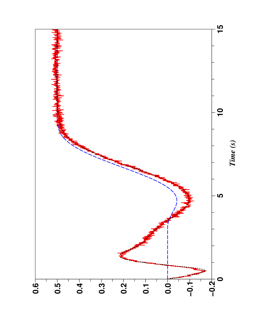
(e) Output (–); reference (- -); denoised output (. .)

Figure 17: The non-minimum phase system where the first effect is not modeled

(a) $u$ (–); $u^{\star}$ (- -)

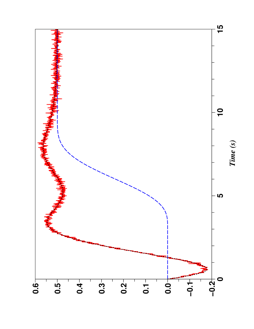
(b) Output (–); reference (- -); denoised output (. .)

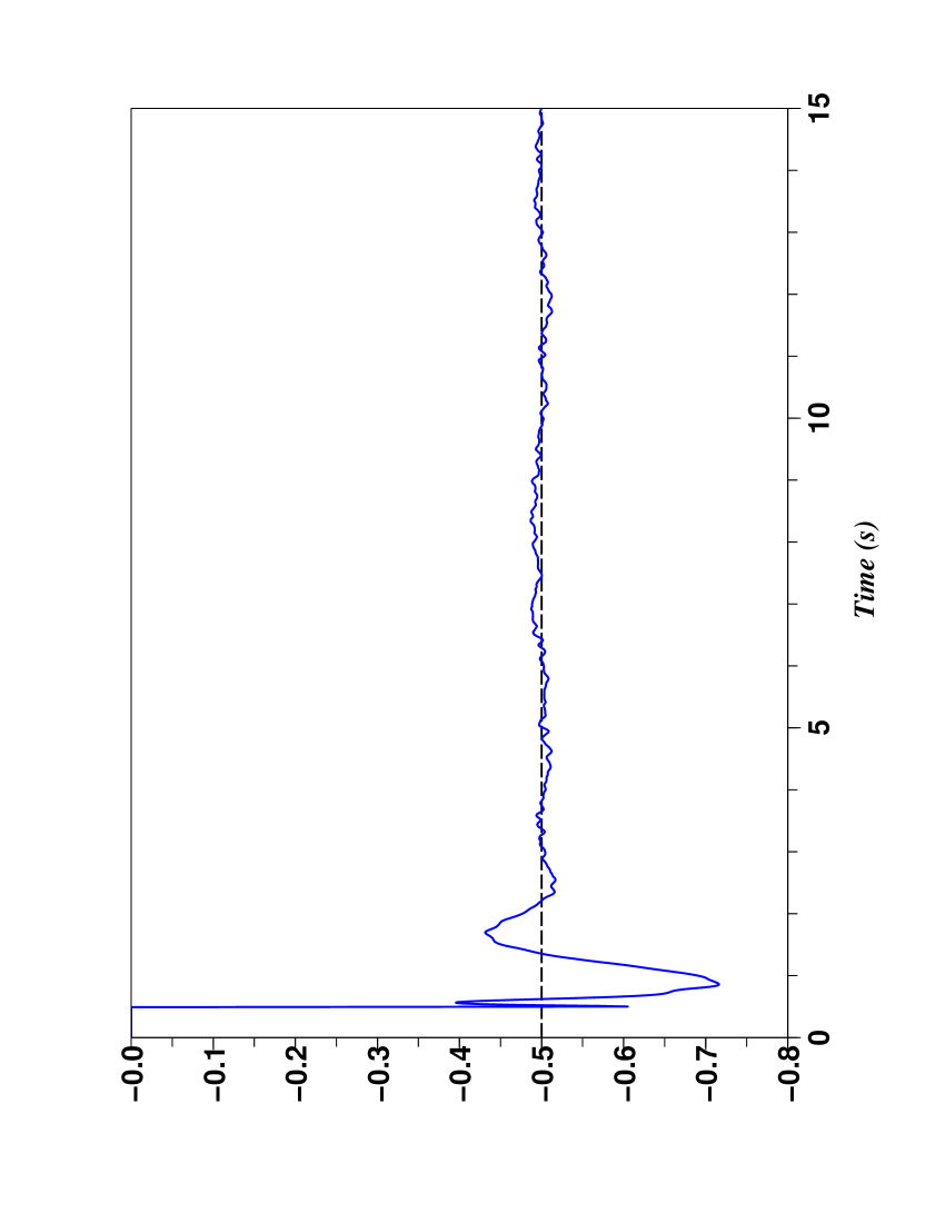
(c) Perturbation (- -); estimated perturbation (–)

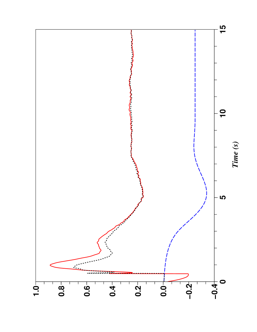
(d) $u$ (–); $u^{\star}$ (- -); $u^{\star}_{\text{pert}}$(. .)

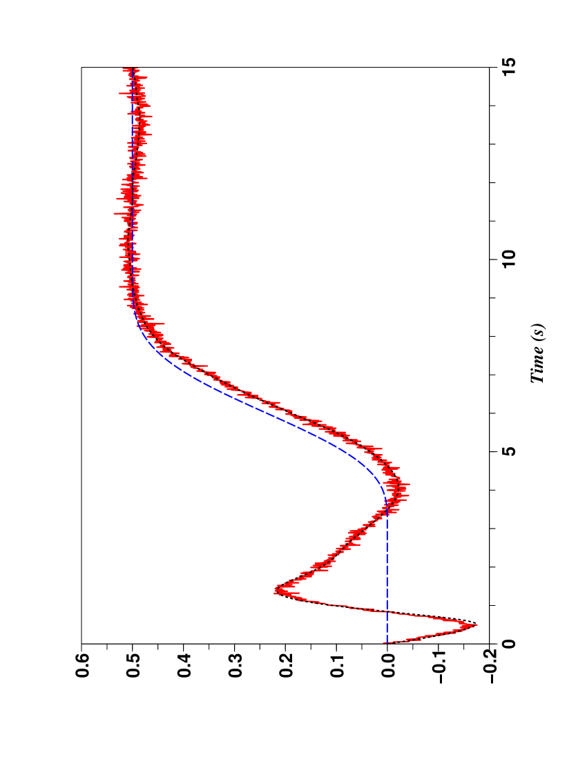
(e) Output (–); reference (- -); denoised output (. .)

Figure 18: The non-minimum phase system where the first effect is not modeled

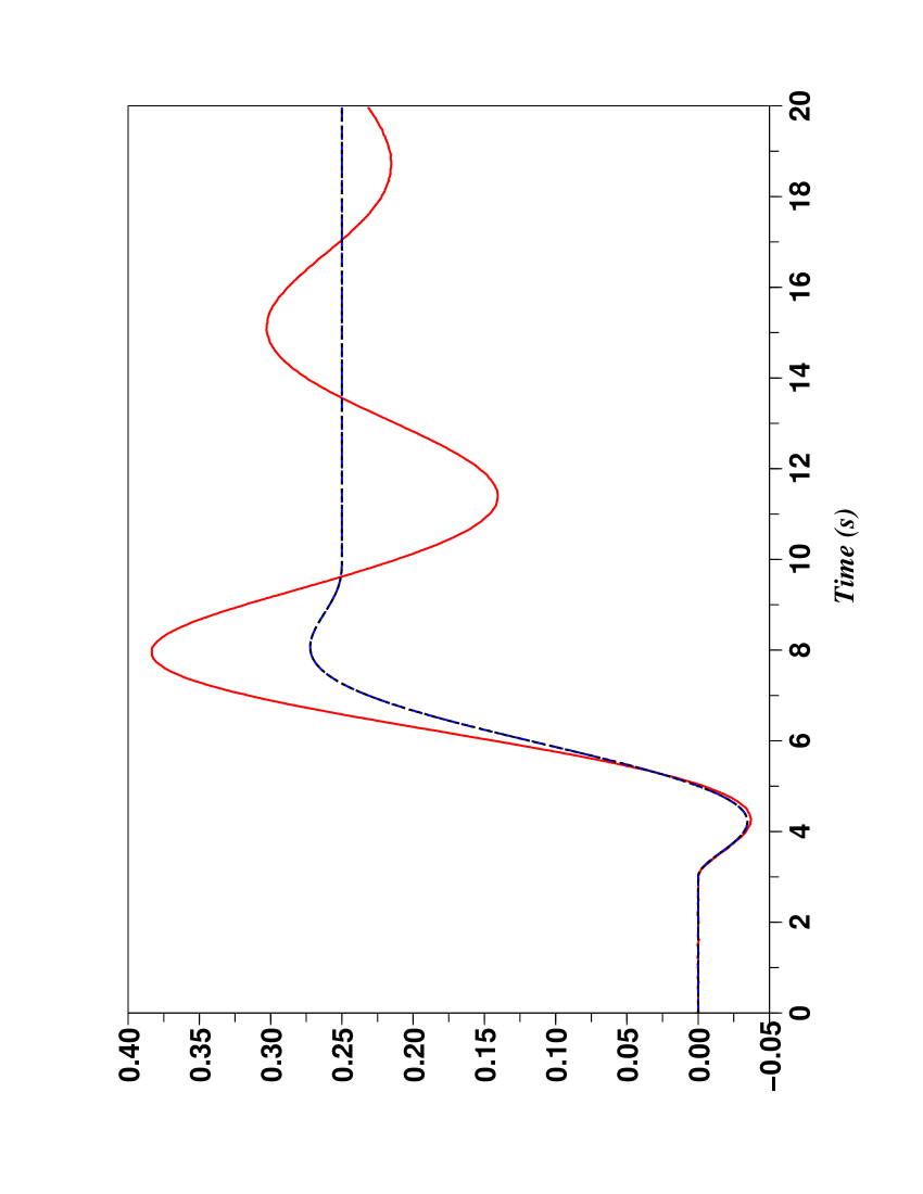
(a) $u$ (–); $u^{\star}$ (- -)

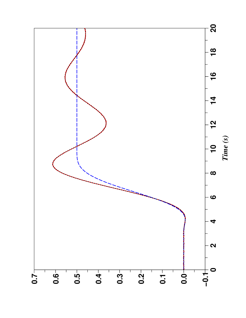
(b) Output (–); reference (- -); denoised output (. .)

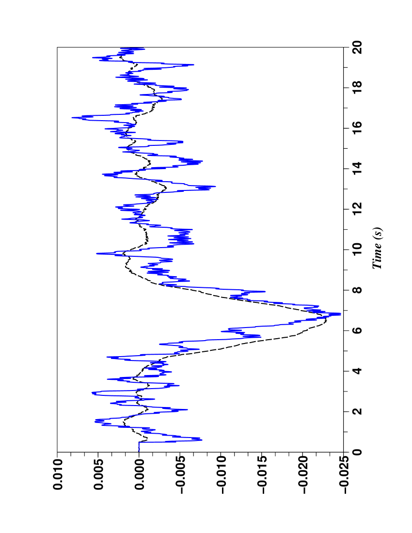
(c) Perturbation (- -); estimated perturbation (–)

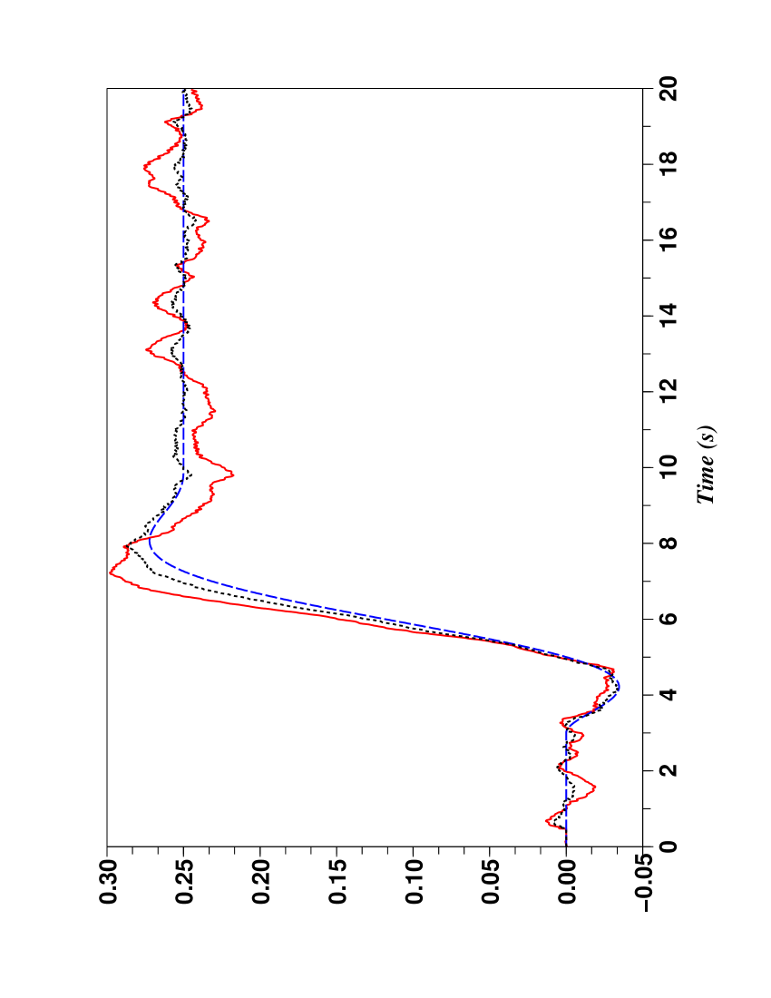
(d) $u$ (–); $u^{\star}$ (- -); $u^{\star}_{\text{pert}}$(. .)

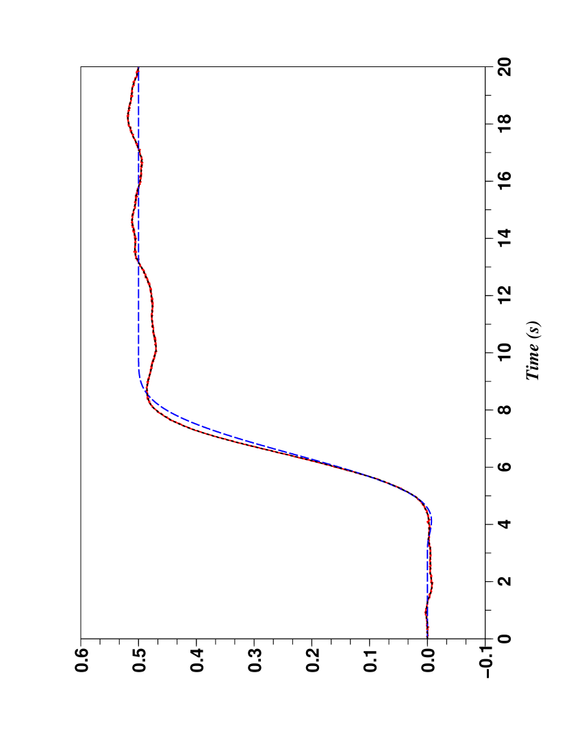
(e) Output (–); reference (- -); denoised output (. .)

Figure 19: The non-minimum phase system where the second effect is not modeled

References

- Antoulas (2005) A.C. Antoulas. Approximation of Large-Scale Dynamical Systems. SIAM, 2005.
- Åström & Hägglund (2006) K.J. Åström, T. Hägglund. Advanced PID Control. Instrument Soc. Amer., 2006.
- Åström, Persson & Hang (1992) K.J. Åström, C.C. Hang, P. Persson, W.K. Ho. Towards intelligent PID control. Automatica, 28:1–9, 1992.
- Åström & Murray (2008) K.J. Åström, R.M. Murray. Feedback Systems: An Introduction for Scientists and Engineers. Princeton University Press, 2008.
- Belkoura, Richard & Fliess (2009) L. Belkoura, J.-P. Richard, M. Fliess. Parameters estimation of systems with delayed and structered entries. Automatica, 2009. Available at http://hal.inria.fr/inria-00343801/en/.
- Besançon-Voda & Gentil (1999) A. Besançon-Voda, S. Gentil. Régulateurs PID analogiques et numériques. Techniques de l’Ingénieur, R7416, 1999.
- Bohn & Atherton (1995) C. Bohn, D.P. Atherton. An analysis package comparing PID anti-windup strategies. IEEE Control Syst. Magaz., 15:34–40, 1995.
- Bourdais, Fliess, Join & Perruquetti (2007) R. Bourdais, M. Fliess, C. Join, W. Perruquetti. Towards a model-free output tracking of switched nonlinear systems Proc. 7th IFAC Symp. Nonlinear Control Systems, Pretoria, 2007. Available at http://hal.inria.fr/inria-00147702/en/.
- Chambert-Loir (2005) A. Chambert-Loir. Algèbre corporelle. Éditions École Polytechnique, 2005. English translation: A Field Guide to Algebra, Springer, 2005.
- Choi, d’Andréa-Novel, Fliess & Mounier (2009) S. Choi, B. d’Andréa-Novel, M. Fliess, H. Mounier. Model-free control of automotive engine and brake for stop-and-go scenario. Proc. 10th IEEE Conf. Europ. Control Conf., Budapest, 2009. Soon available at http://hal.inria.fr/.
- Dattaet, Ho & Bhattacharyya (2000) A. Datta, M.T. Ho, S.P. Bhattacharyya. Structure and Synthesis of PID Controllers. Springer, 2000.
- Delaleau (2002) E. Delaleau. Algèbre différentielle. In J.-P. Richard, editor, Mathématiques pour les systèmes dynamiques, vol. 2, chapter 6, pp. 245–268, Hermès, 2002.
- Delaleau (2008) E. Delaleau. Classical electrical engineering questions in the light of Fliess’s differential algebraic framework of non-linear control systems. Int. J. Control, 81:380–395, 2008.
- Dindeleux (1981) D. Dindeleux. Technique de la regulation industrielle. Eyrolles, 1981.
- Fantoni & Lozano (2002) I. Fantoni, R. Lozano. Non-linear control for underactuated mechanical systems. Springer, 2002.
- Fliess (2006) M. Fliess. Analyse non standard du bruit. C.R. Acad. Sci. Paris Ser. I, 342:797–802, 2006.
- Fliess & Join (2008a) M. Fliess, C. Join. Commande sans modèle et commande à modèle restreint. e-STA, 5 (n∘ 4):1-23, 2008a. Available at http://hal.inria.fr/inria-00288107/en/.
- Fliess & Join (2008b) M. Fliess, C. Join. Time series technical analysis via new fast estimation methods: a preliminary study in mathematical finance. Proc. 23rd IAR Workshop Advanced Control Diagnosis (IAR-ACD08), Coventry, 2008b. Available at http://hal.inria.fr/inria-00338099/en/.
- Fliess & Join (2009a) M. Fliess, C. Join. A mathematical proof of the existence of trends in financial time series. Proc. Int. Conf. Systems Theory: Modelling, Analysis and Control, Fes, 2009a. Available at http://hal.inria.fr/inria-00352834/en/.
- Fliess & Join (2009b) M. Fliess, C. Join. Towards new technical indicators for trading systems and risk management. Proc. 15th IFAC Symp. System Identif. (SYSID 2009), Saint-Malo, 2009b. Available at http://hal.inria.fr/inria-00370168/en/.
- Fliess, Join & Sira-Ramírez (2005) M. Fliess, C. Join, H. Sira-Ramírez. Closed-loop fault-tolerant control for uncertain nonlinear systems. In T. Meurer, K. Graichen and E.D. Gilles editors, Control and Observer Design for Nonlinear Finite and Infinite Dimensional Systems, Lect. Notes Control Informat. Sci., volume 322, pages 217–233, Springer, 2005.
- Fliess, Join & Sira-Ramírez (2008) M. Fliess, C. Join, H. Sira-Ramírez. Non-linear estimation is easy. Int. J. Modelling Identification Control, vol. 4:12–27 (2008). Available at http://hal.inria.fr/inria-00158855/en/.
- Fliess, Lévine, Martin & Rouchon (1995) M. Fliess, J. Lévine, P. Martin, P. Rouchon. Flatness and defect of non-linear systems: introductory theory and examples. Int. J. Control, 61:1327–1361, 1995.
- Fliess & Marquez (2000) M. Fliess, R. Marquez. Continuous-time linear predictive control and flatness: a module-theoretic setting with examples. Int. J. Control, 73:606–623, 2000.
- Fliess, Marquez, Delaleau & Sira-Ramírez (2002) M. Fliess, R. Marquez, E. Delaleau, H. Sira-Ramírez. Correcteurs proportionnels-intégraux généralisés ", ESAIM Control Optim. Calc. Variat., 7:23–41, 2002.
- Fliess, Marquez & Mounier (2002) M. Fliess, R. Marquez, H. Mounier. An extension of predictive control, PID regulators and Smith predictors to some delay systems. Int. J. Control, 75:728–743, 2002.
- Fliess & Sira-Ramírez (2003) M. Fliess, H. Sira-Ramírez. An algebraic framework for linear identification. ESAIM Control Optim. Calc. Variat., 9:151–168, 2003.
- Franklin, Powell & Emami-Naeini (2002) G.F. Franklin, J.D. Powell, A. Emami-Naeini. Feedback Control of Dynamic Systems. 4th edition, Prentice Hall, 2002.
- Gédouin, Join, Delaleau, Bourgeot, Chirani & Calloch (2008) P.-A. Gédouin, C. Join, E. Delaleau, J.-M. Bourgeot, S.A. Chirani, S. Calloch. Model-free control of shape memory alloys antagonistic actuators. Proc. 17th IFAC World Congress (WIFAC-2008), Seoul, 2008. Available at http://hal.inria.fr/inria-00261891/en/.
- Hippe (2006) P. Hippe. Windup in Control - Its Effects and Their Prevention. Springer, 2006.
- Isidori (1999) A. Isidori. Nonlinear Control Systems II. Springer, 1999.
- Johnson & Moradi (2005) M.A. Johnson, M.H. Moradi. PID Control: New Identification and Design Methods. Springer, 2005.
- Join, Masse & Fliess (2008) C. Join, J. Masse, M. Fliess. Étude préliminaire d’une commande sans modèle pour papillon de moteur. J. europ. syst. automat., 42:337–354, 2008. Available at http://hal.inria.fr/inria-00187327/en/.
- Kerschen, Worden, Vakakis & Golinval (2006) G. Kerschen, K. Worden, A.F. Vakakis, J.-C. Golinval. Past, present and future of nonlinear system identification in structural dynamics. Mech. Systems Signal Process., 20:505–592, 2006.
- Hauser, Sastry & Kokotovic (1992) J. Hauser, S. Sastry, P. Kokotović. Nonlinear control via approximate input-output linearization: The ball and beam example. IEEE Trans. Automat. Control, 37:392–398, 1992.
- Kolchin (1973) E.R. Kolchin. Differential Algebra and Algebraic Groups. Academic Press, 1973.
- Lequesne (2006) D. Lequesne. Régulation P.I.D. : analogique - numérique - floue. Hermès, 2006.
- Mboup, Join & Fliess (2009) M. Mboup, C. Join, M. Fliess. Numerical differentiation with annihilators in noisy environment. Numer. Algo., 50, 2009. DOI: 10.1007/s11075-008-9236-1.
- Nuninger, Perruquetti & Richard (2006) W. Nuninger, W. Perruquetti, J.-P. Richard. Bilan et enjeux des modèles de frottements: tribologie et contrôle au service de la sécurité des transports, Actes 5e Journées Europ. Freinage (JEF’2006), Lille, 2006. Available at http://hal.inria.fr/inria-00192425/en/.
- Obinata & Anderson (2001) G. Obinata, B.D.O. Anderson. Model Reduction for Control Systems. Springer, 2001.
- O’Dwyer (2006) A. O’Dwyer. Handbook of PI and PID Controller Tuning Rules. 2nd ed., Imperial College Press, 2006.
- Ollivier, Moutaouakil & Sadik (2007) F. Ollivier, S. Moutaouakil, B. Sadik. Une méthode d’identification pour un système linéaire à retards. C.R. Acad. Sci. Paris Ser. I, 344:709–714, 2007.
- Olsson, Åström, Canudas de Wit, Gäfvert & Lischinsky (1998) H. Olsson, K. J. Åström, C. Canudas de Wit, M. Gäfvert, P. Lischinsky. Friction models and friction compensation. Europ. J. Control, 4:176–195, 1998.
- Peng, Vrancic & Hanus (1996) Y. Peng, D. Vrancic, R. Hanus. Anti-windup, bumpless, and conditioned transfer transfer techniques for PID controllers. IEEE Control Syst. Magaz., 16:48–57,1996.
- Rotella & Zambettakis (2007) F. Rotella, I. Zambettakis. Commande des systèmes par platitude. Techniques de l’ingénieur, S7450, 2007.
- Rotella & Zambettakis (2008) F. Rotella, I. Zambettakis. Automatique élémentaire. Hermès, 2008.
- Rudolph & Woittennek (2007) J. Rudolph, F. Woittennek. Ein algebraischer Zugang zur Parameteridentifkation in linearen unendlichdimensionalen Systemen. at–Automatisierungstechnik, 55:457–467, 2007.
- Sastry (1999) S. Sastry. Nonlinear Systems. Springer, 1999.
- Shinskey (1996) F.G. Shinskey. Process Control Systems - Application, Design, and Tuning. 4th ed., McGraw-Hill, 1996.
- Sira-Ramírez & Agrawal (2004) H. Sira-Ramírez, S. Agrawal. Differentially Flat Systems. Marcel Dekker, 2004.
- Sjöberg, Zhang, Ljung, Benveniste, Delyon, Glorennec, Hjalmarsson & Juditsky (1995) J. Sjöberg, Q. Zhang, L. Ljung, A. Benveniste, B. Delyon, P.-Y. Glorennec, H. Hjalmarsson, A. Juditsky. Nonlinear black-box modeling in system identification: a unified overview. Automatica, 31:1691–1724, 1995.
- Tustin (1947) A. Tustin. The effect of backlash and of speed dependent friction on the stability of closed-cycle control systems. J. Instit. Elec. Eng., 94:143–151, 1947.
- Villagra, d’Andréa-Novel, Fliess & Mounier (2008a) J. Villagra, B. d’Andréa-Novel, M. Fliess, H. Mounier. Estimation of longitudinal and lateral vehicle velocities an algebraic approach. Proc. Amer. Control Conf. (ACC-2008), Seattle, 2008a. Available at http://hal.inria.fr/inria-00263844/en/.
- Villagra, d’Andréa-Novel, Fliess & Mounier (2008b) J. Villagra, B. d’Andréa-Novel, M. Fliess, H. Mounier. Robust grey box closed-loop stop-and-go control. Proc. 47th IEEE Conf. Decision Control, Cancun, 2008. Available at http://hal.inria.fr/inria-00319591/en/.
- Visioli (2006) A. Visioli. Practical PID Control. Springer, 2006.
- Wang, Ye, Cai & Hang (2008) Q.-J. Wang, Z. Ye, W.-J. Cai and C.-C. Hang. PID Control for Multivariable Processes. Springer, 2008.
- Yosida (1984) K. Yosida. Operational Calculus A Theory of Hyperfunctions. Springer, 1984 (translated from the Japanese).
- Yu (1999) C.C. Yu. Autotuning of PID Controllers. Springer, 1999.
- Zhang, Jiang & Wang (2002) Y. Zhang, D. Jiang, J. Wang. A recurrent neural network for solving Sylvester equation with time-varying coefficients. IEEE Trans. Neural Networks, 13:1053–1063, 2002.
- Ziegler & Nichols (1942) J.G. Ziegler, N.B. Nichols. Optimum settings for automatic controllers. Trans. ASME, 64:759–768, 1942.