Superfluid response and the neutrino emissivity of baryon matter: Fermi-liquid effects.

Abstract

The linear response of a nonrelativistic superfluid baryon system on an external weak field is investigated while taking into account of the Fermi-liquid interactions. We generalize the theory developed by Leggett for a superfluid Fermi-liquid at finite temperature to the case of timelike momentum transfer typical of the problem of neutrino emission from neutron stars. A space-like kinematics is also analysed for completeness and compared with known results.

We use the obtained response functions to derive the neutrino energy losses caused by recombination of broken pairs in the electrically neutral superfluid baryon matter. We find that the dominant neutrino radiation occurs through the axial-vector neutral currents. The emissivity is found to be of the same order as in the BCS approximation, but the details of its temperature dependence are modified by the Fermi-liquid interactions.

The role of electromagnetic correlations in the pairing case of protons interacting with the electron background is discussed in the conclusion.

LABEL:FirstPage1

I Introduction

Thermal excitations in superfluid baryon matter of neutron stars, in the form of broken Cooper pairs, can recombine into the condensate by emitting neutrino pairs via neutral weak currents. This process was suggested FRS76 many years ago as an efficient mechanism for cooling of neutron stars in some ranges of temperature and/or matter density. The interest in this process has been recently revived LP06 –SR in connection with the fact that the existing theory of thermal neutrino radiation from superfluid neutron matter leads to a rapid cooling of the neutron star crust, which is in dramatic discrepancy with the observed data of superbursts Cumming , Gupta . It was realized that a better understanding of an efficiency of the neutrino emission in the pair recombination is necessary to explain modern observations.

The relevant input for calculation of neutrino energy losses from the medium is the imaginary part of the retarded weak-polarization tensor intimately connected with the autocorrelation function of weak currents in the medium. Though the theoretical investigation of the autocorrelation functions of strong-interacting superfluid fermions was started more than four decades ago the complete theory of the problem does not yet exist. Leggett’s theory of a superfluid Fermi liquid Leggett is limited to the case when both the transferred energy and momentum are small compared to the superfluid energy gap, i.e., $\omega,\mathrm{q}\ll\Delta$. This theory cannot be applied to calculations of neutrino energy losses because, in this case, we need the medium response onto an external neutrino field in the time-like kinematic domain, $\omega>\mathrm{q}$, and $\omega>2\Delta$, as required by the total energy $\omega=\omega_{1}+\omega_{2}$ and momentum $\mathbf{q=q}_{1}+\mathbf{q}_{2}$ of escaping neutrino pair.

The well-known Larkin-Migdal theory Larkin is restricted to the case of zero temperature. Recently, the calculation of the neutrino energy losses was undertaken in Refs. KV08 , SR , where the imaginary part of the autocorrelation functions was calculated for a superfluid neutron matter at zero temperature. This approach is apparently inconsistent because the imaginary part of retarded polarization functions substantially depends on the temperature [see Eqs. (82), (88), (112), and (113) of this work]. One more inconsistency of the work SR is, that the temporal component of the axial-vector current cannot be discarded, as it is done by the authors. This relativistic correction contributes to the neutrino energy losses of the same order as the spin-density fluctuations, i.e. $\propto V_{F}^{2}$. This was pointed out for the first time in Ref. Kaminker . Below, we will return to the discussion of these works and compare our result with that obtained in Refs. KV08 , SR and in some earlier works.

The appropriate, temperature-dependent approach is developed in Ref. L08 , where the mean-field BCS approximation is used to calculate the superfluid response in the vector channel. To include the Fermi-liquid effects discarded in the BCS approximation, in this paper, we first generalize Leggett’s theory to the case of arbitrary momentum transfer. We evaluate the weak-interaction effective vertices and the autocorrelation functions while taking into account strong residual particle-hole interactions. To obtain a solution of Leggett’s equations in reasonably simple form, we approximate the particle-hole interactions by its first two harmonics with the aid of the usual Landau parameters. Within these constraints we obtain the general expression for the autocorrelation functions and then focus on the superfluid response in the time-like kinematic domain. We investigate both the vector channel and the axial channel of weak interactions to evaluate the rate of neutrino energy loss through neutral weak currents caused by recombination of electrically neutral baryons.

The role of electromagnetic correlations in the pairing case of charged baryons interacting with the electron background deserves a separate consideration. The quantum transitions of charged quasiparticles can excite background electrons, thus inducing the neutrino-pair emission by the electron plasma L00 , L01 . In summary, we briefly discuss this problem in the light of modern theory to understand whether the plasma effects can lead to noticeable neutrino energy losses through the vector channel.

The paper is organized as follows. The next section contains some preliminary notes and outlines some important properties of Green’s functions and the one-loop integrals used below. In Sec. III, we discuss the set of equations derived by Leggett for calculation of correlation functions of a superfluid Fermi liquid at finite temperature. In Sec. IV, we consider the superfluid response in the vector channel. Because of the conservation of the vector weak current it is sufficient to consider only the longitudinal and transverse autocorrelation functions. The correlation functions in the axial channel are evaluated in Sec. V. As an application of our findings, in Sec. VI, we evaluate neutrino energy losses through neutral weak currents caused by the pair recombination in superfluid neutron matter. Some numerical estimates of the neutrino energy losses are represented in Sec. VII. Section VIII contains a short summary of our findings and the conclusion.

In this work we use the standard model of weak interactions, the system of units $\hbar=c=1,$ and the Boltzmann constant $k_{B}=1$.

II Preliminary notes and notation

In our analysis, we will use the fact that the Fermi-liquid interactions do not interfere with the pairing phenomenon if approximate hole-particle symmetry is maintained in the system; i.e. the Fermi-liquid interactions remain unchanged upon pairing. According to Landau’s theory, near the Fermi surface, $\mathsf{p\simeq p}^{\prime}\mathsf{\simeq p}_{F}$, the Fermi-liquid interactions can be reduced to the interactions in the particle-hole channel. We will assume that the effective interaction amplitude is the function of the angle between incoming momenta $\mathbf{p}$ and $\mathbf{p}^{\prime}$ and can be parametrized as the sum of the scalar and exchange terms

$$a^{2}\rho\hat{\Gamma}^{\omega}\left(\mathbf{nn}^{\prime}\right)=f\left(\mathbf{nn}^{\prime}\right)+g\left(\mathbf{nn}^{\prime}\right){\textstyle\sum_{i}}\hat{\sigma}_{i}\hat{\sigma}_{i}^{\prime}.$$ (1)

Here and below, $\rho=\mathrm{p}_{F}M^{\ast}/\pi^{2}$ is the density of states near the Fermi surface; $\mathbf{n}=\mathbf{p/}\mathsf{p}$ and $\mathbf{n}^{\prime}=\mathbf{p}^{\prime}\mathbf{/}\mathsf{p}^{\prime}$ are the unit vectors specifying directions of incoming momenta, $a\simeq 1$ is a usual Green’s function renormalization constant independent of $\omega,\mathbf{q}$, and $T$, and $\hat{\sigma}_{i}$ ($i=1,2,3$) stand for Pauli spin matrices. The pairing interaction, irreducible in the channel of two quasiparticles, is renormalized in the same manner

$$a^{2}\rho\hat{\Gamma}^{\varphi}\left(\mathbf{nn}^{\prime}\right)=\Gamma_{a}^{\varphi}\left(\mathbf{nn}^{\prime}\right)+\Gamma_{b}^{\varphi}\left(\mathbf{nn}^{\prime}\right){\textstyle\sum_{i}}\hat{\sigma}_{i}\hat{\sigma}_{i}^{\prime}.$$ (2)

We will consider the case when the pairing occurs only between two quasiparticles with the total spin $S=0$. Then the irreducible pairing amplitude is to be taken as the singlet,

$$a^{2}\rho\hat{\Gamma}^{\varphi}\left(\mathbf{nn}^{\prime}\right)\rightarrow\Gamma^{\varphi}\left(\mathbf{nn}^{\prime}\right)\equiv\Gamma_{a}^{\varphi}\left(\mathbf{nn}^{\prime}\right)-3\Gamma_{b}^{\varphi}\left(\mathbf{nn}^{\prime}\right).$$ (3)

Since the baryonic component of stellar matter is in thermal equilibrium at some temperature $T$, we adopt the Matsubara Green’s functions for the description of the superfluid condensate and for evaluation of the polarization tensor. In the case of ${}^{1}S_{0}$ pairing, near the Fermi surface, these are given by: AGD :

$$G\left(p_{n},\mathbf{p}\right)=a\frac{-ip_{n}-\varepsilon_{\mathbf{p}}}{p_{n}^{2}+E_{\mathbf{p}}^{2}},\ G_{h}\left(p_{n},\mathbf{p}\right)=a\frac{ip_{n}-\varepsilon_{\mathbf{p}}}{p_{n}^{2}+E_{\mathbf{p}}^{2}},\ F\left(p_{n},\mathbf{p}\right)=a\frac{\Delta}{p_{n}^{2}+E_{\mathbf{p}}^{2}},$$ (4)

where $p_{n}=\pi\left(2n+1\right)T$ with $n=0,\pm 1,\pm 2,...$ is the fermionic Matsubara frequency. In the above equation, $G$ and $G_{h}$ represent the propagators of a particle and of a hole, respectively, and $F$ is the anomalous propagator, i.e. the amplitude of the quasiparticle transition into a hole and a correlated pair. For the inverse process: $F^{\dagger}\left(p_{n},\mathbf{p}\right)=F\left(p_{n},\mathbf{p}\right)$.

We use the momentum representation and the following notation

$$\varepsilon_{\mathbf{p}}=\frac{\mathsf{p}^{2}}{2M^{\ast}}-\frac{\mathsf{p}_{F}^{2}}{2M^{\ast}}\simeq\frac{\mathsf{p}_{F}}{M^{\ast}}(\mathsf{p}-\mathsf{p}_{F}),$$ (5)

where $M^{\ast}=p_{F}/V_{F}$ is the effective mass of a quasiparticle, and the energy of a quasiparticle is

$$E_{\mathbf{p}}=\sqrt{\varepsilon_{\mathbf{p}}^{2}+\Delta^{2}\left(T\right)}.$$ (6)

We designate as $L_{X,X}\left(\omega,\mathbf{q;p}\right)$ the analytical continuation onto the upper-half plane of complex variable $\omega$ of the following Matsubara sums:

$$L_{XX^{\prime}}\left(\omega_{m},\mathbf{p+}\frac{\mathbf{q}}{2}\mathbf{;p-}\frac{\mathbf{q}}{2}\right)=T\sum_{p_{n}}X\left(p_{n}+\omega_{m},\mathbf{p+}\frac{\mathbf{q}}{2}\right)X^{\prime}\left(p_{n},\mathbf{p-}\frac{\mathbf{q}}{2}\right),$$ (7)

where $X,X^{\prime}\in G,F,G^{h}$.

In Leggett’s equations, which we are going to exploit, the spin dependence is already taken into account, and $\sum_{\mathbf{p,\sigma}}$  is everywhere replaced by $2\sum_{\mathbf{p}}$. It is convenient to divide the integration over the momentum space into the integration over the solid angle and over the energy according

$$\int\frac{2d^{3}\mathrm{p}}{\left(2\pi\right)^{3}}\cdot\cdot\cdot=\rho\int\frac{d\mathbf{n}}{4\pi}\int_{-\infty}^{\infty}d\varepsilon_{\mathbf{p}}\cdot\cdot\cdot$$ (8)

and operate with integrals over the quasiparticle energy:

$$\mathcal{I}_{XX^{\prime}}\left(\omega,\mathrm{q}\cos\theta,T\right)\equiv\int_{-\infty}^{\infty}d\varepsilon_{\mathbf{p}}L_{XX^{\prime}}\left(\omega,\mathbf{p+}\frac{\mathbf{q}}{2}\mathbf{,p-}\frac{\mathbf{q}}{2}\right).$$ (9)

These are functions of $\omega$, $\mathrm{q,}$ and $\cos\theta=\mathbf{nn}_{\mathbf{q}}$, which is the polar angle of the direction of the momentum $\mathbf{p}=\mathrm{p}\mathbf{n}$ relative to the direction of $\mathbf{n}_{\mathbf{q}}=\mathbf{q}/\mathrm{q}$ as the $z$ axis.

The functions $\mathcal{I}_{XX^{\prime}}$ possess the following properties, which can be derived by a straightforward calculation Leggett $:$

$$\mathcal{I}_{GF}=-\mathcal{I}_{FG},\ \mathcal{I}_{FG_{h}}=-\mathcal{I}_{G_{h}F},$$ (10)

$$\mathcal{I}_{G_{h}F}+\mathcal{I}_{FG}=\frac{\omega}{\Delta}\mathcal{I}_{FF},$$ (11)

$$\mathcal{I}_{G_{h}F}-\mathcal{I}_{FG}=-\frac{\mathbf{qv}}{\Delta}\mathcal{I}_{FF},$$ (12)

$$-\left(\mathcal{I}_{GG_{h}}+\mathcal{I}_{FF}\right)=A_{0}+\frac{\left(\mathbf{qv}\right)^{2}-\omega^{2}}{2\Delta^{2}}\mathcal{I}_{FF}.$$ (13)

Here $\mathbf{v=}V_{F}\mathbf{n}$, and the quantity $A_{0}=-\left(\mathcal{I}_{GG_{h}}+\mathcal{I}_{FF}\right)_{\mathbf{q}=0,\omega=0}$ satisfies the gap equation

$$1-\Gamma_{0}^{\varphi}A_{0}=0,$$ (14)

where $\Gamma_{0}^{\varphi}$ is the zeroth harmonic of the singlet pairing amplitude (3).

The key role in the medium response theory belongs to the functions defined as the following combinations of the above loop integrals:

$$\lambda\left(\omega,\mathbf{qn}\right)\equiv a^{-2}\mathcal{I}_{FF},$$ (15)

$$\kappa\left(\omega,\mathbf{qn}\right)\equiv a^{-2}\left(\frac{1}{2}\left(\mathcal{I}_{GG}+\mathcal{I}_{G^{h}G^{h}}\right)+\mathcal{I}_{FF}\right),$$ (16)

$$\chi\left(\omega,\mathbf{qn}\right)\equiv a^{-2}\frac{1}{2}\left(\mathcal{I}_{GG}-\mathcal{I}_{G^{h}G^{h}}\right).$$ (17)

These can be derived in the following form:

$$\lambda=-\frac{\Delta^{2}}{4}\int_{-\infty}^{\infty}\frac{d\varepsilon_{\mathbf{p}}}{E_{+}E_{-}}\left[\left(E_{\mathbf{+}}+E_{\mathbf{-}}\right)\Phi_{+}-\left(E_{\mathbf{+}}-E_{\mathbf{-}}\right)\Phi_{-}\right],$$ (18)

$$\kappa=\frac{\mathbf{qv}}{4}\int_{-\infty}^{\infty}\frac{d\varepsilon_{\mathbf{p}}}{E_{+}E_{-}}\left[\left(E_{\mathbf{-}}\varepsilon_{\mathbf{+}}-\varepsilon_{\mathbf{-}}E_{\mathbf{+}}\right)\Phi_{+}+\left(\varepsilon_{\mathbf{-}}E_{\mathbf{+}}+E_{\mathbf{-}}\varepsilon_{\mathbf{+}}\right)\Phi_{-}\right],$$ (19)

$$\chi=\frac{\omega}{4}\int_{-\infty}^{\infty}\frac{d\varepsilon_{\mathbf{p}}}{E_{+}E_{-}}\left[\left(E_{\mathbf{-}}\varepsilon_{\mathbf{+}}-\varepsilon_{\mathbf{-}}E_{\mathbf{+}}\right)\Phi_{+}+\left(\varepsilon_{\mathbf{-}}E_{\mathbf{+}}+E_{\mathbf{-}}\varepsilon_{\mathbf{+}}\right)\Phi_{-}\right].$$ (20)

To shorten the expressions, we use the following notation:

$$\varepsilon_{\pm}\equiv\varepsilon_{\mathbf{p\pm}\frac{\mathbf{q}}{2}},\ E_{\pm}\equiv E_{\mathbf{p\pm}\frac{\mathbf{q}}{2}},$$ (21)

and

$$\Phi_{\pm}=\frac{1}{\left(\omega+i0\right)^{2}-\left(E_{\mathbf{+}}\pm E_{\mathbf{-}}\right)^{2}}\left(\tanh\frac{E_{\mathbf{+}}}{2T}\pm\tanh\frac{E_{\mathbf{-}}}{2T}\right).$$ (22)

It is straightforward to verify that

$$\lambda\left(\omega,\mathbf{qn}\right)=\lambda\left(\omega,-\mathbf{qn}\right),\ \kappa\left(\omega,\mathbf{qn}\right)=\kappa\left(\omega,-\mathbf{qn}\right),$$ (23)

and that the functions $\kappa\left(\omega,\mathbf{qn}\right)$ and $\chi\left(\omega,\mathbf{qn}\right)$ are not independent because

$$\omega\kappa=\mathbf{qv}\chi.$$ (24)

III Leggett’s finite-temperature formalism

The two-particle autocorrelation function is defined as

$$K_{\xi}\left(\omega,\mathbf{q}\right)\equiv\sum_{\mathbf{pp}^{\prime},\sigma\sigma^{\prime}}\xi\left(\mathbf{p,}\sigma\right)\left\langle\left\langle a_{\mathbf{p+q/}2\mathbf{,}\sigma}^{\dagger}a_{\mathbf{p-q/}2\mathbf{,}\sigma}:a_{\mathbf{p}^{\prime}\mathbf{-q/}2\mathbf{,}\sigma^{\prime}}^{\dagger}a_{\mathbf{p}^{\prime}\mathbf{+q/}2\mathbf{,}\sigma^{\prime}}\right\rangle\right\rangle_{\omega}\xi\left(\mathbf{p}^{\prime}\mathbf{,}\sigma^{\prime}\right),$$ (25)

where $\xi\left(\mathbf{p,}\sigma\right)$ is a three-point vertex responsible for the interaction of a free particle with the weak external field. It is some function of the momentum $\mathbf{p}$ and spin variables $\sigma$; $\left\langle\left\langle A:B\right\rangle\right\rangle_{\omega}$ is the Fourier transform of a retarded two-particle Green’s function.

The analytic form of the autocorrelation function can be immediately written, if we know the effective (full) three-point vertices defined via the linear correction to the quasiparticle self-energy $\Xi^{\left(1\right)}\left(V\right)$ in the external field $V$ (see, e.g., Ref. Migdal ):

$$\mathcal{T}=\xi\left(\mathbf{p,}\sigma\right)+\frac{\partial\Xi^{\left(1\right)}}{\partial V}.$$ (26)

Near the Fermi surface, these vertices can be treated as functions of transferred energy and momentum, $q=\left(\omega,\mathbf{q}\right)$, and the direction of nucleon motion $\mathbf{n}$.

In superfluids, we have to distinguish the vertices of a particle and a hole, which are related as $\xi_{h}\left(\mathbf{p,}\sigma\right)=\xi\left(-\mathbf{p,-}\sigma\right)$. Since there are two possible cases, $\xi\left(-\mathbf{p,-}\sigma\right)=\pm\xi\left(\mathbf{p,}\sigma\right)$, it is convenient to consider the ”even” and ”odd” bare vertices

$$\xi_{\pm}\left(\mathbf{n}\right)=\frac{1}{2}\left(\xi\left(\mathbf{p,}\sigma\right)\pm\xi\left(-\mathbf{p,-}\sigma\right)\right).$$ (27)

We denote as

$$\mathcal{T}_{\pm}\left(\mathbf{n}\right)=\frac{1}{2}\left(\mathcal{T}\left(\mathbf{p,}\sigma\right)\pm\mathcal{T}\left(-\mathbf{p,-}\sigma\right)\right)$$ (28)

the corresponding full vertices taking into account the polarization of superfluid Fermi liquid under the influence of the external field.

In Eq. (26), the quasiparticle self-energy consists of the normal part and the anomalous part caused by the pair condensation. In the case of ${}^{1}S_{0}$ pairing, the anomalous self-energy is sensitive only to the longitudinal vector fields, because the only kind of motion possible for the condensate is potential flow, i.e., a density fluctuation Bogoliubov . Therefore for the longitudinal currents, along with the ordinary vertices $\mathcal{T}_{\pm}$, it is necessary to consider the anomalous vertex $\mathcal{\tilde{T}}$, responsible for excitations of the condensate.

As was derived by Leggett (see Eqs. (22) and (23) of Ref. Leggett ), the longitudinal effective vertices $\mathcal{T}_{\pm},\mathcal{\tilde{T}}$ are to be found from the following equations (we omit for brevity the dependence of functions on $\omega$ and $\mathbf{q}$):

$$\mathcal{\tilde{T}}\left(\mathbf{n}\right)-\int\frac{d\mathbf{n}^{\prime}}{4\pi}\Gamma^{\varphi}\left(\mathbf{nn}^{\prime}\right)A_{0}\mathcal{\tilde{T}}\left(\mathbf{n}^{\prime}\right)-\int\frac{d\mathbf{n}^{\prime}}{4\pi}\Gamma^{\varphi}\left(\mathbf{nn}^{\prime}\right)\frac{\left(\mathbf{qv}^{\prime}\right)^{2}-\omega^{2}}{2\Delta^{2}}\lambda\left(\mathbf{n}^{\prime}\right)\mathcal{\tilde{T}}\left(\mathbf{n}^{\prime}\right)$$

$$+\int\frac{d\mathbf{n}^{\prime}}{4\pi}\Gamma^{\varphi}\left(\mathbf{nn}^{\prime}\right)\frac{\mathbf{qv}^{\prime}}{\Delta}\lambda\left(\mathbf{n}^{\prime}\right)\mathcal{T}_{-}\left(\mathbf{n}^{\prime}\right)-\frac{\omega}{\Delta}\int\frac{d\mathbf{n}^{\prime}}{4\pi}\Gamma^{\varphi}\left(\mathbf{nn}^{\prime}\right)\lambda\left(\mathbf{n}^{\prime}\right)\mathcal{T}_{+}\left(\mathbf{n}^{\prime}\right)=0,$$ (29)

$$\mathcal{T}_{-}\left(\mathbf{n}\right)+\int\frac{d\mathbf{n}^{\prime}}{4\pi}f\left(\mathbf{nn}^{\prime}\right)\frac{\mathbf{qv}^{\prime}}{\Delta}\lambda\left(\mathbf{n}^{\prime}\right)\mathcal{\tilde{T}}\left(\mathbf{n}^{\prime}\right)-\int\frac{d\mathbf{n}^{\prime}}{4\pi}f\left(\mathbf{nn}^{\prime}\right)\kappa\left(\mathbf{n}^{\prime}\right)\mathcal{T}_{-}\left(\mathbf{n}^{\prime}\right)$$

$$+\int\frac{d\mathbf{n}^{\prime}}{4\pi}f\left(\mathbf{nn}^{\prime}\right)\frac{\omega}{\mathbf{qv}^{\prime}}\kappa\left(\mathbf{n}^{\prime}\right)\mathcal{T}_{+}\left(\mathbf{n}^{\prime}\right)=\xi_{-}\left(\mathbf{n}\right),$$ (30)

$$\mathcal{T}_{+}\left(\mathbf{n}\right)-\frac{\mathrm{\omega}}{\Delta}\int\frac{d\mathbf{n}^{\prime}}{4\pi}f\left(\mathbf{nn}^{\prime}\right)\lambda\left(\mathbf{n}^{\prime}\right)\mathcal{\tilde{T}}\left(\mathbf{n}^{\prime}\right)+\int\frac{d\mathbf{n}^{\prime}}{4\pi}f\left(\mathbf{nn}^{\prime}\right)\frac{\omega}{\mathbf{qv}^{\prime}}\kappa\left(\mathbf{n}^{\prime}\right)\mathcal{T}_{-}\left(\mathbf{n}^{\prime}\right)$$

$$-\int\frac{d\mathbf{n}^{\prime}}{4\pi}f\left(\mathbf{nn}^{\prime}\right)\left(\kappa\left(\mathbf{n}^{\prime}\right)-2\lambda\left(\mathbf{n}^{\prime}\right)\right)\mathcal{T}_{+}\left(\mathbf{n}^{\prime}\right)=\xi_{+}\left(\mathbf{n}\right).$$ (31)

In Eq. (29), the irreducible pairing amplitude is to be taken as the singlet, as given by Eq. (3).

Once the effective vertices are calculated, the two-particle autocorrelation function can be immediately found using the expressions:

$$K_{\xi}=\rho\int\frac{d\mathbf{n}}{4\pi}\xi_{+}\left(\mathbf{n}\right)\left[\frac{\omega}{\Delta}\lambda\left(\mathbf{n}\right)\mathcal{\tilde{T}}\left(\mathbf{n}\right)+\frac{\omega}{\mathbf{qv}}\kappa\left(\mathbf{n}\right)\mathcal{T}_{-}\left(\mathbf{n}\right)+\left(\kappa\left(\mathbf{n}\right)-2\lambda\left(\mathbf{n}\right)\right)\mathcal{T}_{+}\left(\mathbf{n}\right)\right],$$ (32)

if $\xi=\xi_{+}$, and

$$K_{\xi}=\rho\int\frac{d\mathbf{n}}{4\pi}\xi_{-}\left(\mathbf{n}\right)\left[-\frac{\mathbf{qv}}{\Delta}\lambda\left(\mathbf{n}\right)\mathcal{\tilde{T}}\left(\mathbf{n}\right)+\kappa\left(\mathbf{n}\right)\mathcal{T}_{-}\left(\mathbf{n}\right)-\frac{\omega}{\mathbf{qv}}\kappa\left(\mathbf{n}\right)\mathcal{T}_{+}\left(\mathbf{n}\right)\right]$$ (33)

if $\xi=\xi_{-}$.

One can easily verify that these equations represent a generalization for the case of finite temperatures of the Larkin-Migdal Larkin equations derived in the ladder approximation for the vertices modified by strong interactions in a superfluid Fermi liquid.

Unless we are dealing with a spin-independent longitudinal field only fluctuations of the normal component contribute to the polarization. The corresponding effective vertices should be found from the equations Leggett :

$$\mathcal{T}_{-}\left(\mathbf{n}\right)-\int\frac{d\mathbf{n}^{\prime}}{4\pi}\Gamma^{\omega}\left(\mathbf{nn}^{\prime}\right)\left[\kappa\left(\mathbf{n}^{\prime}\right)\mathcal{T}_{-}\left(\mathbf{n}^{\prime}\right)-\frac{\omega}{\mathbf{qv}^{\prime}}\kappa\left(\mathbf{n}^{\prime}\right)\mathcal{T}_{+}\left(\mathbf{n}^{\prime}\right)\right]=\xi_{-}\left(\mathbf{n}\right),$$ (34)

$$\mathcal{T}_{+}\left(\mathbf{n}\right)+\int\frac{d\mathbf{n}^{\prime}}{4\pi}\Gamma^{\omega}\left(\mathbf{nn}^{\prime}\right)\left[\frac{\omega}{\mathbf{qv}^{\prime}}\kappa\left(\mathbf{n}^{\prime}\right)\mathcal{T}_{-}\left(\mathbf{n}^{\prime}\right)-\left(\kappa\left(\mathbf{n}^{\prime}\right)-2\lambda\left(\mathbf{n}^{\prime}\right)\right)\mathcal{T}_{+}\left(\mathbf{n}^{\prime}\right)\right]=\xi_{+}\left(\mathbf{n}\right),$$ (35)

which represent Dyson’s equations ideally summing the particle-hole irreducible diagrams in the ladder approximation. In these equations, the spin dependence is already taken into account, so $\xi$ is to be taken as a function of only $\mathbf{p}$, i.e. $\xi\left(\mathbf{p}\right)\equiv\xi\left(\mathbf{p,}\sigma\right)=\xi\left(\mathbf{p,-}\sigma\right)$ for $S=0$, and $\xi\left(\mathbf{p}\right)\equiv\xi\left(\mathbf{p,}\sigma\right)=-\xi\left(\mathbf{p,-}\sigma\right)$ for $S=1$. The $c$ number $\Gamma^{\omega}$ refers to the usual Landau ”quasiparticle-irreducible” scattering amplitude $\Gamma^{\omega}\left(\mathbf{n,n}^{\prime}\right)$ as defined in the normal phase; it is to be taken as the spin-independent or spin-dependent part according to $\xi\left(\mathbf{p,}\sigma\right)=\pm\xi\left(\mathbf{p,-}\sigma\right)$.

In this way one may calculate the spin, transverse-current, and helicity-current autocorrelation functions, which are given by the expressions:

$$K_{\xi}=\rho\int\frac{d\mathbf{n}}{4\pi}\xi_{+}\left(\mathbf{n}\right)\left[\frac{\omega}{\mathbf{qv}}\kappa\left(\mathbf{n}\right)\mathcal{T}_{-}\left(\mathbf{n}\right)+\left(\kappa\left(\mathbf{n}\right)-2\lambda\left(\mathbf{n}\right)\right)\mathcal{T}_{+}\left(\mathbf{n}\right)\right],$$ (36)

if $\xi=\xi_{+}$, and

$$K_{\xi}=\rho\int\frac{d\mathbf{n}}{4\pi}\xi_{-}\left(\mathbf{n}\right)\left[\kappa\left(\mathbf{n}\right)\mathcal{T}_{-}\left(\mathbf{n}\right)-\frac{\omega}{\mathbf{qv}}\kappa\left(\mathbf{n}\right)\mathcal{T}_{+}\left(\mathbf{n}\right)\right]$$ (37)

if $\xi=\xi_{-}$.

We are now in a position to evaluate the autocorrelation functions necessary for calculating the energy losses from a hot superfluid baryon matter. We consider the medium response in the vector and axial-vector channels which are responsible for the neutrino interactions with the medium through neutral weak currents.

IV Vector channel

Vector current of a quasiparticle $J^{\mu}$ is a vector in Dirac space $\left(\mu=0,1,2,3\right)$. The corresponding polarization tensor $\Pi_{\mathrm{V}}^{\mu\nu}\left(\omega,\mathbf{q}\right)$ must obey the current conservation conditions:

$$\Pi_{\mathrm{V}}^{\mu\nu}\left(\omega,\mathbf{q}\right)q_{\nu}=0,\ q_{\mu}\Pi_{\mathrm{V}}^{\mu\nu}\left(\omega,\mathbf{q}\right)=0.$$ (38)

These equations imply that the polarization tensor can be represented as the sum of longitudinal (with respect to $\mathbf{q}$) and transverse components

$$\Pi_{\mathrm{V}}^{\mu\nu}\left(\omega,\mathbf{q}\right)=\Pi_{L}\left(\omega,\mathbf{q}\right)\left(1,\frac{\omega}{\mathsf{q}}\mathbf{n}_{\mathbf{q}}\right)^{\mu}\left(1,\frac{\omega}{\mathsf{q}}\mathbf{n}_{\mathbf{q}}\right)^{\nu}+\Pi_{T}\left(\omega,\mathbf{q}\right)g^{\mu i}\left(\delta^{ij}-n_{\mathbf{q}}^{i}n_{\mathbf{q}}^{j}\right)g^{j\nu}.$$ (39)

In this expansion, the longitudinal and transverse polarization functions are defined as

$$\Pi_{L}=\Pi^{00},\ \ \ \ \Pi_{T}=\frac{1}{2}\left(\delta^{ij}-n_{\mathbf{q}}^{i}n_{\mathbf{q}}^{j}\right)\Pi^{ij}.$$ (40)

The transverse polarization function can be conveniently evaluated in the reference frame where the $z$ axis is pointed along the transferred momentum, so that $\mathbf{n}_{\mathbf{q}}=\left(0,0,1\right)$. Then

$$\Pi_{T}\left(\omega,\mathbf{q}\right)=\frac{1}{2}\left(\Pi^{1,1}\left(\omega,\mathbf{q}\right)+\Pi^{2,2}\left(\omega,\mathbf{q}\right)\right).$$ (41)

Thus we actually need to calculate only the temporal and transverse components of the effective vertices.

IV.1 Longitudinal polarization

The vector current of a free particle has the nonrelativistic form

$$j_{V}^{\mu}=\left(1,\bm{v}\right),$$ (42)

where $\bm{v}=\mathbf{p/}M$ is the particle velocity. In this case we find

$$\xi^{0}=\xi_{+}^{0}=1,\ \ \ \ \ \xi_{-}^{0}=0,$$ (43)

$$\mathbf{\xi}_{+}^{i}=0,\ \ \ \ \mathbf{\xi}^{i}=\mathbf{\xi}_{-}^{i}=\bm{v}^{i}.$$ (44)

Then the longitudinal polarization, $\Pi_{L}=K_{1}\left(\omega,\mathbf{q}\right),$can be calculated with the aid of Eqs. (29)-(32) with $\xi_{+}=1$ and $\xi_{-}=0$.

Before proceeding to the detailed solution of these equations, let us note that apart from the ground state, Eq. (29) allows for excitations of the bound pairs with the orbital momentum $l>0$, if these exist. We will consider the simplest case of ${}^{1}S_{0}$ pairing, assuming that the only possible bound state of the pair corresponds to the zero angular momentum $l$. This allows us to consider only the zeroth harmonic of the pairing interaction. In this case the anomalous vertex is independent of the quasiparticle momentum and the use of the gap equation (14) allows us to recast Eq. (29) as follows:

$$\mathcal{\tilde{T}}\int\frac{d\mathbf{n}}{4\pi}\left(\omega^{2}-\left(\mathbf{qv}\right)^{2}\right)\lambda\left(\mathbf{n}\right)=2\Delta\int\frac{d\mathbf{n}}{4\pi}\left(\omega\lambda\left(\mathbf{n}\right)\mathcal{T}_{+}\left(\mathbf{n}^{\prime}\right)-\left(\mathbf{qv}\right)\lambda\left(\mathbf{n}\right)\mathcal{T}_{-}\left(\mathbf{n}\right)\right).$$ (45)

Using Eq. (43), we obtain Eqs. (30) and (31) in the form

$$\mathcal{T}_{-}\left(\mathbf{n}\right)+\int\frac{d\mathbf{n}^{\prime}}{4\pi}f\left(\mathbf{nn}^{\prime}\right)\frac{\mathbf{qv}^{\prime}}{\Delta}\lambda\left(\mathbf{n}^{\prime}\right)\mathcal{\tilde{T}}\left(\mathbf{n}^{\prime}\right)-\int\frac{d\mathbf{n}^{\prime}}{4\pi}f\left(\mathbf{nn}^{\prime}\right)\kappa\left(\mathbf{n}^{\prime}\right)\mathcal{T}_{-}\left(\mathbf{n}^{\prime}\right)$$

$$+\int\frac{d\mathbf{n}^{\prime}}{4\pi}f\left(\mathbf{nn}^{\prime}\right)\frac{\omega}{\mathbf{qv}^{\prime}}\kappa\left(\mathbf{n}^{\prime}\right)\mathcal{T}_{+}\left(\mathbf{n}^{\prime}\right)=0,$$ (46)

$$\mathcal{T}_{+}\left(\mathbf{n}\right)-\frac{\mathrm{\omega}}{\Delta}\int\frac{d\mathbf{n}^{\prime}}{4\pi}f\left(\mathbf{nn}^{\prime}\right)\lambda\left(\mathbf{n}^{\prime}\right)\mathcal{\tilde{T}}\left(\mathbf{n}^{\prime}\right)+\int\frac{d\mathbf{n}^{\prime}}{4\pi}f\left(\mathbf{nn}^{\prime}\right)\frac{\omega}{\mathbf{qv}^{\prime}}\kappa\left(\mathbf{n}^{\prime}\right)\mathcal{T}_{-}\left(\mathbf{n}^{\prime}\right)$$

$$-\int\frac{d\mathbf{n}^{\prime}}{4\pi}f\left(\mathbf{nn}^{\prime}\right)\left(\kappa\left(\mathbf{n}^{\prime}\right)-2\lambda\left(\mathbf{n}^{\prime}\right)\right)\mathcal{T}_{+}\left(\mathbf{n}^{\prime}\right)=1.$$ (47)

The vertex equations can be further simplified in various assumptions about the amplitude of the particle-hole interaction (1), which can be expanded in the Legendre polynomials, according to

$$f\left(\mathbf{nn}^{\prime}\right)=\sum_{l}f_{l}P_{l}\left(\mathbf{nn}^{\prime}\right).$$ (48)

We consider a simplified model with $f_{l}=0$ for $l\geq 2$, when the interaction function is given as

$$f\left(\mathbf{nn}^{\prime}\right)=f_{0}+f_{1}\mathbf{nn}^{\prime}.$$ (49)

Solution to the set of Eqs. (45)–(47) can be written with the aid of the following notation:

$$\alpha\left(\omega,\mathrm{q},T\right) \equiv\int\frac{d\mathbf{n}}{4\pi}\lambda\left(\mathbf{n}\right),\ \gamma\left(\omega,\mathrm{q},T\right)\equiv\int\frac{d\mathbf{n}}{4\pi}\lambda\left(\mathbf{n}\right)\cos^{2}\theta,$$

$$\eta\left(\omega,\mathrm{q},T\right) \equiv\int\frac{d\mathbf{n}}{4\pi}\kappa\left(\mathbf{n}\right),\ \beta\left(\omega,\mathrm{q},T\right)\equiv\int\frac{d\mathbf{n}}{4\pi}\kappa\left(\mathbf{n}\right)\cos^{2}\theta,$$ (50)

$$Q\equiv\eta+\frac{2\alpha\gamma}{s^{2}\alpha-\gamma},\ P\equiv\beta+\frac{2\gamma^{2}}{s^{2}\alpha-\gamma},$$

where

$$s=\frac{\omega}{\mathrm{q}V_{F}}.$$ (51)

After some algebra, we find:

$$\mathcal{T}_{+}=\frac{1-f_{1}P}{1-f_{0}\left(1+f_{1}\left(s^{2}Q-P\right)\right)Q\allowbreak-f_{1}P},$$ (52)

$$\mathcal{T}_{-}=-\frac{sf_{1}Q\cos\theta}{1-f_{0}\left(1+f_{1}\left(s^{2}Q-P\right)\right)Q\allowbreak-f_{1}P},$$ (53)

$$\mathcal{\tilde{T}}=2\frac{\Delta}{\omega}\frac{s^{2}\left(\alpha\left(1-f_{1}\beta\right)+\gamma\eta f_{1}\right)}{\left(s^{2}\alpha-\gamma\right)\left[1-f_{0}\left(1+f_{1}\left(s^{2}Q-P\right)\right)Q\allowbreak-f_{1}P\right]}.$$ (54)

A short calculation of the right-hand side of Eq. (32) with $\xi_{+}=1$ gives the simple result

$$\Pi_{L}\left(\omega,\mathrm{q},T\right)=\rho\frac{\left(1+f_{1}\left(s^{2}Q-P\right)\right)Q\allowbreak}{1-f_{0}\left(1+f_{1}\left(s^{2}Q-P\right)\right)Q\allowbreak-f_{1}P}$$ (55)

IV.1.1 BCS limit.

Notice that the autocorrelation function of the density fluctuations has already been calculated in various limits. Let us take, for example, the BCS limit by setting $f_{0}=f_{1}=0$. We then obtain

$$\Pi_{L}^{\mathrm{BCS}}\left(\omega,\mathrm{q},T\right)=\rho Q\allowbreak\equiv\rho\left(\eta-2\alpha+\frac{2\omega^{2}\alpha^{2}}{\omega^{2}\alpha-\mathrm{q}^{2}V_{F}^{2}\gamma}\right).$$ (56)

This expression is in agreement with Eq. (37) of Ref. L08 if we take into account the relations $\eta-2\alpha=\Lambda_{00}$, $\omega\alpha=-\Delta\Lambda_{0}$, and $\mathrm{q}^{2}V_{F}^{2}\gamma=\Delta q_{i}\Lambda_{i}$ connecting our notations and those of Ref. L08 .

IV.1.2 Limit $\omega,\mathrm{q}V_{F}\ll\Delta$, $T>0$.

In this limiting case, from Eqs. (18), (19), and (50) we find (see also Ref. Leggett )

$$\alpha\simeq\frac{1}{2}+\frac{1}{2}\int\frac{d\mathbf{n}}{4\pi}\int_{0}^{\infty}d\varepsilon\frac{\left(\cos^{2}\theta-s^{2}\right)\varepsilon^{2}/E^{2}}{s^{2}-\left(\cos^{2}\theta\right)\varepsilon^{2}/E^{2}}\frac{dn}{dE},$$ (57)

$$\gamma\simeq\frac{1}{6}+\frac{1}{2}\int\frac{d\mathbf{n}}{4\pi}\int_{0}^{\infty}d\varepsilon\frac{\cos^{2}\theta\ \left(\cos^{2}\theta-s^{2}\right)\varepsilon^{2}/E^{2}}{s^{2}-\left(\cos^{2}\theta\right)\varepsilon^{2}/E^{2}}\frac{dn}{dE},$$ (58)

$$\eta\simeq\int\frac{d\mathbf{n}}{4\pi}\int_{0}^{\infty}d\varepsilon\frac{\left(\cos^{2}\theta\right)\varepsilon^{2}/E^{2}}{s^{2}-\left(\cos^{2}\theta\right)\varepsilon^{2}/E^{2}}\frac{dn}{dE},$$ (59)

$$\beta\simeq 2\gamma+s^{2}\eta-\frac{1}{3},$$ (60)

$$P\simeq s^{2}Q-\frac{1}{3},$$ (61)

where

$$\frac{dn}{dE}=\frac{1}{2T}\cosh^{-2}\frac{E}{2T}.$$ (62)

Then Eq. (55) gives

$$\Pi_{L}\left(\omega,\mathrm{q}V_{F}\ll\Delta,T\right)=\frac{\rho Q\left(s\right)}{1-\left[f_{0}+f_{1}s^{2}/\left(1+f_{1}/3\right)\right]Q\left(s\right)},$$ (63)

in agreement with the result of Leggett Leggett .

IV.1.3 Limit $\omega,\mathrm{q}V_{F}\ll\Delta$, $T=0$.

In the case $T=0$, Eqs. (57)–(60) give

$$\alpha=\frac{1}{2},\ \gamma=\frac{1}{6},\eta=\beta=0,$$ (64)

so

$$Q=\frac{1}{3s^{2}-1},\ P=\frac{1}{3}Q.$$ (65)

We then obtain

$$\Pi_{L}\left(\omega,\mathrm{q}V_{F}\ll\Delta,T=0\right)=\frac{\rho\left(1+f_{1}/3\right)\mathrm{q}^{2}V_{F}^{2}/3.}{\omega^{2}-\left(1+f_{0}\right)\left(1+f_{1}/3\right)\mathrm{q}^{2}V_{F}^{2}/3}.$$ (66)

in agreement with the results obtained in Ref. Larkin .

IV.1.4 Time-like momentum transfer, $0<T<T_{c}$

We are interested in the case of time-like momentum transfer, $\mathrm{q}<\omega,$ and $\omega>2\Delta$ taking place in kinematics of the neutrino-pair emission. Then we deal with the case $\mathrm{q}V_{F}\ll\omega$, i.e., $u\equiv s^{-1}\ll 1$. In this limit, we have

$$\operatorname{Re}\gamma=\frac{1}{3}\operatorname{Re}\alpha,\ \beta\sim\eta\sim u^{2}\alpha,$$ (67)

Using this fact, we find the functions $Q$ and $P$ in the forms

$$Q=\eta+2u^{2}\gamma,$$ (68)

$$s^{2}Q-P=s^{2}\eta-\beta+2\gamma$$ (69)

The real and imaginary parts of the functions can be obtained from Eqs. (18), (19), and (50). The real part can be evaluated to the lowest accuracy. We find:

$$\operatorname{Re}\alpha=-\mathcal{P}\int_{-\infty}^{\infty}\frac{d\varepsilon}{E}\frac{\Delta^{2}}{\omega^{2}-4E^{2}}\tanh\frac{E}{2T},$$ (70)

$$\operatorname{Re}\gamma=-\frac{1}{3}\mathcal{P}\int_{-\infty}^{\infty}\frac{d\varepsilon}{E}\frac{\Delta^{2}}{\omega^{2}-4E^{2}}\tanh\frac{E}{2T},$$ (71)

$$\operatorname{Re}\eta=\frac{u^{2}}{3}\left(1+2\mathcal{P}\int_{-\infty}^{\infty}\frac{d\varepsilon}{E}\frac{\allowbreak\Delta^{2}}{\omega^{2}-4E^{2}}\tanh\frac{E}{2T}\right),$$ (72)

$$\operatorname{Re}\beta=\frac{u^{2}}{5}\left(1+2\mathcal{P}\int_{-\infty}^{\infty}\frac{d\varepsilon}{E}\frac{\allowbreak\Delta^{2}}{\omega^{2}-4E^{2}}\tanh\frac{E}{2T}\right),$$ (73)

where the symbol $\mathcal{P}$ means principal value of the integral. In deriving the last two equalities we used the identity

$$\frac{1}{2}\int_{-\infty}^{\infty}\frac{d\varepsilon}{E}\frac{\Delta^{2}}{E^{2}}\tanh\frac{E}{2T}+\frac{1}{2}\int_{-\infty}^{\infty}d\varepsilon\frac{\varepsilon^{2}}{E^{2}}\frac{dn}{dE}=1.$$ (74)

Within a time-like momentum transfer and $\omega>2\Delta$, the imaginary part of the function arises because of the pole at $\omega=E_{\mathbf{p+q}}+E_{\mathbf{p}}$. We calculate the imaginary contributions up to the higher accuracy and find

$$\operatorname{Im}\alpha =\pi\frac{\Delta^{2}}{\omega\sqrt{\omega^{2}-4\Delta^{2}}}\Theta\left(\omega-2\Delta\right)\tanh\frac{\omega}{4T}$$

$$\times\left(\allowbreak 1+\frac{1}{3}u^{2}\left(\frac{\omega^{2}+4\Delta^{2}}{\omega^{2}-4\Delta^{2}}\allowbreak-\frac{\omega^{2}-4\Delta^{2}}{16T^{2}}\cosh^{-2}\frac{\omega}{4T}\right)\allowbreak\right),$$ (75)

$$\operatorname{Im}\gamma =\frac{\pi}{3}\frac{\Delta^{2}}{\omega\sqrt{\omega^{2}-4\Delta^{2}}}\Theta\left(\omega-2\Delta\right)\tanh\frac{\omega}{4T}$$

$$\times\left(1\allowbreak+\frac{3}{5}u^{2}\left(\frac{8\Delta^{2}+\omega^{2}}{\omega^{2}-4\Delta^{2}}-\frac{\omega^{2}-4\Delta^{2}}{16T^{2}}\cosh^{-2}\frac{\omega}{4T}\allowbreak\right)\allowbreak\allowbreak\right)$$ (76)

$$\operatorname{Im}\eta =-\frac{2\pi}{3}\frac{u^{2}\Delta^{2}}{\omega\sqrt{\omega^{2}-4\Delta^{2}}}\Theta\left(\omega-2\Delta\right)\tanh\frac{\omega}{4T}$$

$$\times\left(1+\frac{6}{5}u^{2}\left(\frac{\omega^{2}+2\Delta^{2}}{\omega^{2}-4\Delta^{2}}-\frac{\omega^{2}-4\Delta^{2}}{32T^{2}}\cosh^{-2}\frac{\omega}{4T}\right)\right)\allowbreak,$$ (77)

$$\operatorname{Im}\beta =-\frac{2\pi}{5}\frac{u^{2}\Delta^{2}}{\omega\sqrt{\omega^{2}-4\Delta^{2}}}\Theta\left(\omega-2\Delta\right)\tanh\frac{\omega}{4T}$$

$$\times\left(\allowbreak 1+\frac{25}{28}u^{2}\left(\allowbreak\frac{\omega^{2}+4\Delta^{2}}{\omega^{2}-4\Delta^{2}}\allowbreak-\allowbreak\frac{\omega^{2}-4\Delta^{2}}{80T^{2}}\cosh^{-2}\frac{\omega}{4T}\allowbreak\allowbreak\allowbreak\allowbreak\right)\right),$$ (78)

where $\Theta\left(x\right)$ is the ordinary Heaviside step function.

We also find:

$$Q=\frac{u^{2}}{3}-i\frac{2\pi}{5}\frac{u^{4}\Delta^{2}\Theta\left(\omega-2\Delta\right)}{\omega\sqrt{\omega^{2}-4\Delta^{2}}}\tanh\frac{\omega}{4T},$$ (79)

$$s^{2}Q-P =\frac{1}{3}+i\frac{5\pi}{14}\frac{u^{4}\Delta^{2}\Theta\left(\omega-2\Delta\right)}{\omega\left(\omega^{2}-4\Delta^{2}\right)\sqrt{\omega^{2}-4\Delta^{2}}}\tanh\frac{\omega}{4T}$$

$$\times\left(\allowbreak\frac{\omega^{2}+4\Delta^{2}}{\omega^{2}-4\Delta^{2}}\allowbreak-\allowbreak\frac{\omega^{2}-4\Delta^{2}}{80T^{2}}\cosh^{-2}\frac{\omega}{4T}\allowbreak\allowbreak\allowbreak\allowbreak\right),$$ (80)

and

$$P =\frac{u^{2}}{5}\left(1+\frac{8}{9}\mathcal{P}\int_{-\infty}^{\infty}\frac{d\varepsilon}{E}\frac{\allowbreak\Delta^{2}}{\omega^{2}-4E^{2}}\tanh\frac{E}{2T}\right)$$

$$-i\frac{2\pi}{5}\frac{u^{2}\Delta^{2}\Theta\left(\omega-2\Delta\right)}{\omega\sqrt{\omega^{2}-4\Delta^{2}}}\tanh\frac{\omega}{4T}.$$ (81)

Having these formulas at hand, we can evaluate the real and imaginary parts of the longitudinal polarization function (55). After a little algebra, we obtain

$$\Pi_{L}\left(\omega,\mathrm{q},T\right) =\rho\frac{1}{3}V_{F}^{2}\left(1+\frac{1}{3}f_{1}\right)\frac{\mathrm{q}^{2}}{\omega^{2}}$$

$$-i\frac{2\pi}{5}\rho V_{F}^{4}\left(1+\frac{1}{3}f_{1}\right)^{2}\frac{\mathrm{q}^{4}\Delta^{2}\Theta\left(\omega-2\Delta\right)}{\omega^{5}\sqrt{\omega^{2}-4\Delta^{2}}}\tanh\frac{\omega}{4T},$$ (82)

As one can see from this expression the spherical harmonic of the pairing interaction does not affect the longitudinal polarization in the high-frequency limit $\omega\gg\mathrm{q}V_{F}$. If we set $f_{1}=0$, this expression reproduces the result of the BCS approximation [see Eq. (48) in Ref. L08 ].

IV.2 Transverse polarization

As explained above, the transverse field does not affect the anomalous self-energy of a quasiparticle. Therefore the transverse-current autocorrelation function

$$K_{T}\left(\omega,\mathrm{q}\right)=\frac{1}{2}\left(K_{\xi_{-}=v_{1}}\left(\omega,\mathrm{q}\right)+K_{\xi_{-}=v_{2}}\left(\omega,\mathrm{q}\right)\right).$$ (83)

can be evaluated with the aid of Eqs. (34), (35), and (37) with $\xi_{+}=0$ and $\xi_{-}^{i}=v_{\perp}^{i}$, where $\bm{v}_{\perp}=\left(v\sin\theta\cos\varphi,v\sin\theta\sin\varphi,0\right)$. The particle-hole interaction (49) can be written as

$$f_{0}+f_{1}\mathbf{nn}^{\prime}\equiv f_{0}+f_{1}\left(\cos\theta\cos\theta^{\prime}+\sin\theta\sin\theta^{\prime}\cos\left(\varphi-\varphi^{\prime}\right)\right).$$ (84)

The sets of equations for different $i=\left(1,2\right)$ are decoupled, and we find:

$$\mathcal{T}_{+}^{\left(i\right)}\left(\mathbf{n}\right)=0,\ \mathcal{T}_{-}^{\left(i\right)}=\frac{v_{\perp}^{\left(i\right)}}{1+f_{1}\left(\eta-\beta\right)/2}$$ (85)

and

$$K_{T}\left(\omega,\mathrm{q}\right)=\frac{\rho}{2}\frac{V_{F}^{2}\left(\eta-\beta\right)}{1+f_{1}\left(\eta-\beta\right)/2}$$ (86)

In the case $\mathrm{q}<\omega,$ and $\omega>2\Delta$, using Eqs. (72), (73), (77), and (78), we find

$$\eta-\beta =\frac{2}{15}u^{2}\left(1+2\mathcal{P}\int_{-\infty}^{\infty}\frac{d\varepsilon}{E}\frac{\allowbreak\Delta^{2}}{\omega^{2}-4E^{2}}\tanh\frac{E}{2T}\right)$$

$$-i\frac{4\pi}{15}\frac{u^{2}\Delta^{2}}{\omega\sqrt{\omega^{2}-4\Delta^{2}}}\tanh\frac{\omega}{4T}.$$ (87)

Up to accuracy $V_{F}^{4}$ from Eq. (86), we obtain

$$K_{T}\left(\omega,\mathrm{q}\right) =\frac{1}{15}\rho V_{F}^{4}\frac{\mathrm{q}^{2}}{\omega^{2}}\left(1+2\mathcal{P}\int_{-\infty}^{\infty}\frac{d\varepsilon}{E}\frac{\allowbreak\Delta^{2}}{\omega^{2}-4E^{2}}\tanh\frac{E}{2T}\right)$$

$$-i\frac{2\pi}{15}\rho V_{F}^{4}\frac{\mathrm{q}^{2}\Delta^{2}}{\omega^{3}\sqrt{\omega^{2}-4\Delta^{2}}}\tanh\frac{\omega}{4T}.$$ (88)

This expression coincides with that of the BCS approximation L08 . We see that in the high-frequency limit, $u\ll 1,$ the first two harmonics of the particle-hole interaction do not affect the transverse polarization of the medium.

V Axial channel

Since only the normal component contributes to the spin fluctuations, the axial effective vertices should be found from Eqs. (34) and (35), and the corresponding correlation functions are given by Eqs. (36) and (37). We now focus on this calculation.

The operator of the axial-vector current is a Dirac pseudovector. For a free particle, it is of the nonrelativistic form $\left(\mu=0,1,2,3\right)$

$$\hat{\jmath}_{A}^{\mu}=\left({\textstyle\sum_{i}}\hat{\sigma}_{i}v_{i}\mathbf{,}\hat{\sigma}_{1}\mathbf{,}\hat{\sigma}_{2}\mathbf{,}\hat{\sigma}_{3}\right),$$ (89)

where $\bm{v}=\mathbf{p}/M$ is the particle velocity, and $\hat{\sigma}_{i}$ are Pauli spin matrices. For $S=1$, the exchange part of the particle-hole interaction is to be taken as

$$g\left(\mathbf{nn}^{\prime}\right){\textstyle\sum_{i}}\hat{\sigma}_{i}\hat{\sigma}_{i}^{\prime}=\frac{1}{4}g\left(\mathbf{nn}^{\prime}\right),$$ (90)

and

$$\xi_{+}^{\mu}=v\delta_{\mu 0},\ \xi_{-}^{\mu}=\delta_{\mu,i}.$$ (91)

Then for a space part of the correlation tensor ($i,j=1,2,3$) we find $K_{A}^{ij}=\delta_{ij}K_{A}$, where

$$K_{A}\left(\omega,\mathrm{q}\right)=\rho\int\frac{d\mathbf{n}}{4\pi}\left[\kappa\left(\mathbf{n}\right)\mathcal{T}_{-}\left(\mathbf{n}\right)-\frac{\omega}{\mathbf{qv}}\kappa\left(\mathbf{n}\right)\mathcal{T}_{+}\left(\mathbf{n}\right)\right],$$ (92)

and the full vertices are to satisfy the equations

$$\mathcal{T}_{-}\left(\mathbf{n}\right)-\frac{1}{4}\int\frac{d\mathbf{n}^{\prime}}{4\pi}g\left(\mathbf{nn}^{\prime}\right)\left[\kappa\left(\mathbf{n}^{\prime}\right)\mathcal{T}_{-}\left(\mathbf{n}^{\prime}\right)-\frac{\omega}{\mathbf{qv}^{\prime}}\kappa\left(\mathbf{n}^{\prime}\right)\mathcal{T}_{+}\left(\mathbf{n}^{\prime}\right)\right]=1,$$ (93)

$$\mathcal{T}_{+}\left(\mathbf{n}\right)+\frac{1}{4}\int\frac{d\mathbf{n}^{\prime}}{4\pi}g\left(\mathbf{nn}^{\prime}\right)\left[\frac{\omega}{\mathbf{qv}^{\prime}}\kappa\left(\mathbf{n}^{\prime}\right)\mathcal{T}_{-}\left(\mathbf{n}^{\prime}\right)-\left(\kappa\left(\mathbf{n}^{\prime}\right)-2\lambda\left(\mathbf{n}^{\prime}\right)\right)\mathcal{T}_{+}\left(\mathbf{n}^{\prime}\right)\right]=0.$$ (94)

The temporal component is of the form:

$$K_{A}^{00}\left(\omega,\mathrm{q}\right)=\rho v\int\frac{d\mathbf{n}}{4\pi}\left[\frac{\omega}{\mathbf{qv}}\kappa\left(\mathbf{n}\right)\mathcal{T}_{-}^{0}\left(\mathbf{n}\right)+\left(\kappa\left(\mathbf{n}\right)-2\lambda\left(\mathbf{n}\right)\right)\mathcal{T}_{+}^{0}\left(\mathbf{n}\right)\right],$$ (95)

where the full vertices should be found from the following set of equations

$$\mathcal{T}_{-}^{0}\left(\mathbf{n}\right)-\frac{1}{4}\int\frac{d\mathbf{n}^{\prime}}{4\pi}g\left(\mathbf{nn}^{\prime}\right)\left[\kappa\left(\mathbf{n}^{\prime}\right)\mathcal{T}_{-}^{0}\left(\mathbf{n}^{\prime}\right)-\frac{\omega}{\mathbf{qv}^{\prime}}\kappa\left(\mathbf{n}^{\prime}\right)\mathcal{T}_{+}^{0}\left(\mathbf{n}^{\prime}\right)\right]=0,$$ (96)

$$\mathcal{T}_{+}^{0}\left(\mathbf{n}\right)+\frac{1}{4}\int\frac{d\mathbf{n}^{\prime}}{4\pi}g\left(\mathbf{nn}^{\prime}\right)\left[\frac{\omega}{\mathbf{qv}^{\prime}}\kappa\left(\mathbf{n}^{\prime}\right)\mathcal{T}_{-}^{0}\left(\mathbf{n}^{\prime}\right)-\left(\kappa\left(\mathbf{n}^{\prime}\right)-2\lambda\left(\mathbf{n}^{\prime}\right)\right)\mathcal{T}_{+}^{0}\left(\mathbf{n}^{\prime}\right)\right]=v.$$ (97)

Mixed space-time components are given by

$$K_{A}^{0i}\left(\omega,\mathrm{q}\right)=\rho v\int\frac{d\mathbf{n}}{4\pi}\left[\frac{\omega}{\mathbf{qv}}\kappa\left(\mathbf{n}\right)\mathcal{T}_{-}\left(\mathbf{n}\right)+\left(\kappa\left(\mathbf{n}\right)-2\lambda\left(\mathbf{n}\right)\right)\mathcal{T}_{+}\left(\mathbf{n}\right)\right],$$ (98)

$$K_{A}^{i0}\left(\omega,\mathrm{q}\right)=\rho\int\frac{d\mathbf{n}}{4\pi}\left[\kappa\left(\mathbf{n}\right)\mathcal{T}_{-}^{0}\left(\mathbf{n}\right)-\frac{\omega}{\mathbf{qv}}\kappa\left(\mathbf{n}\right)\mathcal{T}_{+}^{0}\left(\mathbf{n}\right)\right].$$ (99)

To obtain a solution in reasonably simple form, we approximate the interaction amplitude by its first two harmonics, according $g\left(\mathbf{nn}^{\prime}\right)\equiv g_{0}+g_{1}\mathbf{nn}^{\prime}$. Then we find the full vertices in the form

$$\mathcal{T}_{+}^{0} =\frac{v}{1+g_{0}\left(2\alpha-\eta\left(1+B_{1}s^{2}\eta\right)\right)/4},$$

$$\mathcal{T}_{-}^{0}\left(\mathbf{n}\right) =-\frac{vB_{1}s\eta\cos\theta}{1+g_{0}\left(2\alpha-\eta\left(1+B_{1}s^{2}\eta\right)\right)/4},$$ (100)

$$\mathcal{T}_{+}\left(\mathbf{n}\right) =-\frac{B_{2}\eta s\cos\theta}{1-g_{0}\eta\left(1+B_{2}s^{2}\eta\right)/4},$$

$$\mathcal{T}_{-} =\frac{1}{1-g_{0}\eta\left(1+B_{2}s^{2}\eta\right)/4},$$ (101)

where

$$B_{1}\left(\omega,\mathrm{q}\right)\equiv\frac{1}{4}g_{1}\left(1-\frac{1}{4}g_{1}\beta\right)^{-1},$$ (102)

$$B_{2}\left(\omega,\mathrm{q}\right)\equiv\frac{1}{4}g_{1}\left(1-\frac{1}{4}g_{1}\left(\beta-2\gamma\right)\right)^{-1}.$$ (103)

Simple algebraic calculations yield the following autocorrelation functions:

$$K_{A}^{00}\left(\omega,\mathrm{q}\right)=-\rho v^{2}\frac{2\alpha-\eta\left(1-B_{1}s^{2}\eta\right)}{1+g_{0}\left(2\alpha-\eta\left(1+B_{1}s^{2}\eta\right)\right)/4},$$ (104)

and

$$K_{A}^{ij}\left(\omega,\mathrm{q}\right)=\delta_{ij}\rho\frac{\eta\left(1+B_{2}s^{2}\eta\right)}{1-g_{0}\eta\left(1+B_{2}s^{2}\eta\right)/4},$$ (105)

Mixed components $K_{A}^{0i}$ and $K_{A}^{i0}$ are given by the integrals (95) and (99), where, according to Eqs. (23), (100) and (101), the integrands are odd in $\cos\theta$. Therefore the mixed polarization vanishes:

$$K_{A}^{0i}\left(\omega,\mathrm{q}\right)=K_{A}^{i0}\left(\omega,\mathrm{q}\right)=0.$$ (106)

Let us consider various limits in the expressions obtained above. For arbitrary temperature $T>0$ and $\omega,\mathrm{q}V_{F}\ll\Delta$, according to Eq. (60), we have

$$\beta=2\gamma+s^{2}\eta-\frac{1}{3},$$ (107)

and

$$B_{2}=\frac{1}{4}g_{1}\frac{1}{1-g_{1}\left(s^{2}\eta-\frac{1}{3}\right)/4}.$$ (108)

Then the spin-density autocorrelation function (105) reproduces the result obtained in Ref. Leggett

$$K_{A}^{ij}\left(\omega,\mathrm{q}\right)=\delta_{ij}\rho\frac{\eta\left(s\right)}{1-\eta\left(s\right)J\left(s\right)},$$ (109)

where

$$J\left(s\right)=\frac{1}{4}\left(g_{0}+\frac{s^{2}g_{1}}{1+g_{1}/12}\right),$$ (110)

and $\eta\left(s\right)$ is given by Eq. (59).

Next we consider the case of time-like momentum transfer when $\mathrm{q}V_{F}\ll\Delta$, $\omega>2\Delta$, and thus $u\equiv s^{-1}\ll 1$. From Eqs. (70), (71) and (75), (76), we find in this limit

$$\gamma\left(\omega,T\right)\simeq\frac{1}{3}\alpha\left(\omega,T\right).$$ (111)

For $\omega>0$, we obtain

$$\operatorname{Im}K_{A}^{00}\left(\omega,\mathrm{q}\right)\simeq-2\pi\rho v^{2}\frac{\Delta^{2}}{\omega\sqrt{\omega^{2}-4\Delta^{2}}}\frac{\Theta\left(\omega-2\Delta\right)}{\left|1+g_{0}\alpha\left(\omega,T\right)/2\right|^{2}}\tanh\frac{\omega}{4T},$$ (112)

and

$$\operatorname{Im}K_{A}^{ij}\left(\omega,\mathrm{q}\right)=-\delta_{ij}\frac{2\pi}{3}\rho V_{F}^{2}\frac{\mathrm{q}^{2}\Delta^{2}\Theta\left(\omega-2\Delta\right)}{\omega^{3}\sqrt{\omega^{2}-4\Delta^{2}}}\frac{\left(1+g_{1}/12\right)^{2}}{\left|1+g_{1}\alpha\left(\omega,T\right)/6\right|^{2}}\tanh\frac{\omega}{4T},$$ (113)

where

$$\alpha\left(\omega,T\right)=-\mathcal{P}\int_{-\infty}^{\infty}\frac{d\varepsilon}{E}\frac{\Delta^{2}}{\omega^{2}-4E^{2}}\tanh\frac{E}{2T}+i\pi\frac{\Delta^{2}\Theta\left(\omega-2\Delta\right)}{\omega\sqrt{\omega^{2}-4\Delta^{2}}}\tanh\frac{\omega}{4T}.$$ (114)

VI Neutrino energy losses caused by pair recombination

As an application of the obtained results we consider the neutrino-pair emission through neutral weak currents occurring at the recombination of quasiparticles into the ${}^{1}S_{0}$ condensate. The process is kinematically allowed thanks to the existence of a superfluid energy gap $\Delta$, which admits the quasiparticle transitions with time-like momentum transfer $q=\left(\omega,\mathbf{q}\right)$, as required by the final neutrino pair.

We consider the total energy which is emitted into neutrino pairs per unit volume and time which is given by the following formula (see details, e.g., in Ref. L01 ):

$$\epsilon=-\left(\frac{G_{F}}{2\sqrt{2}}\right)^{2}\sum_{\nu}\int\omega\;\frac{2\ \mathrm{Im}\Pi_{\mathrm{weak}}^{\mu\nu}\left(q\right)\ \mathrm{Tr}\left(l_{\mu}l_{\nu}^{\ast}\right)}{\exp\left(\frac{\omega}{T}\right)-1}\frac{d^{3}q_{1}}{2\omega_{1}(2\pi)^{3}}\frac{d^{3}q_{2}}{2\omega_{2}(2\pi)^{3}},$$ (115)

where $G_{F}$ is the Fermi coupling constant, $l_{\mu}$ is the neutrino weak current, and $\Pi_{\mathrm{weak}}^{\mu\nu}$ is the retarded weak polarization tensor of the medium. The integration goes over the phase volume of neutrinos and antineutrinos of total energy $\omega=\omega_{1}+\omega_{2}$ and total momentum $\mathbf{q=q}_{1}+\mathbf{q}_{2}$. The symbol $\sum_{\nu}$  indicates that summation over the three neutrino types has to be performed.

By inserting $\int d^{4}q\delta^{\left(4\right)}\left(q-q_{1}-q_{2}\right)=1$ in this equation, and making use of the Lenard’s integral

$$\int\frac{d^{3}q_{1}}{2\omega_{1}}\frac{d^{3}q_{2}}{2\omega_{2}}\delta^{\left(4\right)}\left(q-q_{1}-q_{2}\right)\mathrm{Tr}\left(l_{\mu}l_{\nu}^{\ast}\right)=\frac{4\pi}{3}\left(q_{\mu}q_{\nu}-q^{2}g_{\mu\nu}\right)\Theta\left(q^{2}\right)\Theta\left(\omega\right),$$ (116)

where $g_{\mu\nu}=\mathsf{\mathrm{diag}}(1,-1,-1,-1)$ is the signature tensor, we can write

$$\epsilon=-\frac{G_{F}^{2}\mathcal{N}_{\nu}}{48\pi^{4}}\int_{0}^{\infty}d\omega\int_{0}^{\omega}d\mathrm{q}\;\mathrm{q}^{2}\frac{\omega}{\exp\left(\frac{\omega}{T}\right)-1}\mathrm{Im}\Pi_{\mathrm{weak}}^{\mu\nu}\left(q\right)\left(q_{\mu}q_{\nu}-q^{2}g_{\mu\nu}\right),$$ (117)

where $\mathcal{N}_{\nu}=3$ is the number of neutrino flavors.

In general, the weak polarization tensor of the medium is a sum of the vector-vector, axial-axial, and mixed terms. However, the medium polarization in the vector channel can be neglected, because the imaginary part of the longitudinal and transverse polarization functions is proportional to $V_{F}^{4}\lll 1$, as given by Eqs. (82) and (88). (See also Refs. LP06 , L08 for details). The mixed axial-vector polarization has to be an antisymmetric tensor, and its contraction in Eq. (117) with the symmetric tensor $q_{\mu}q_{\nu}-q^{2}g_{\mu\nu}$ vanishes. Thus only polarization in the axial channel should be taken into account.

We then obtain $\mathrm{Im}\Pi_{\mathrm{weak}}^{\mu\nu}\simeq C_{A}^{2}\mathrm{Im}K_{A}^{\mu\nu}$, where $C_{A}$ is the axial weak coupling constant of the baryon. Making use of Eqs. (106), (112), and (113), we find

$$\mathrm{Im}\Pi^{\mu\nu}\left(q\right)\left(q_{\mu}q_{\nu}-q^{2}g_{\mu\nu}\right)=-\frac{2}{\pi}C_{A}^{2}p_{F}M^{\ast}V_{F}^{2}\frac{\Delta^{2}\Theta\left(\omega-2\Delta\right)}{\omega\sqrt{\omega^{2}-4\Delta^{2}}}\tanh\frac{\omega}{4T}$$

$$\times\mathrm{q}^{2}\left(\frac{M^{\ast 2}}{M^{2}}\frac{\left(1+g_{1}/12\right)^{2}}{\left|1+g_{0}\alpha\left(\omega,T\right)/2\right|^{2}}+\frac{1}{\left|1+g_{1}\alpha\left(\omega,T\right)/6\right|^{2}}\left(1-\frac{2}{3}\frac{\mathrm{q}^{2}}{\omega^{2}}\right)\right).$$ (118)

By inserting this into Eq. (117) and performing integration over $d\mathrm{q}$, we obtain the neutrino emissivity in the axial channel, which can be represented in the form

$$\epsilon =\frac{4}{15\pi^{5}}G_{F}^{2}C_{A}^{2}\mathcal{N}_{\nu}p_{F}M^{\ast}V_{F}^{2}T^{7}y^{2}\int_{0}^{\infty}dx\frac{z^{4}}{\left(e^{z}+1\right)^{2}}$$

$$\times\left(\frac{M^{\ast 2}}{M^{2}}\frac{\left(1+g_{1}/12\right)^{2}}{\left|1+g_{0}\alpha\left(y,z\right)/2\right|^{2}}+\frac{11}{21}\frac{1}{\left|1+g_{1}\alpha\left(y,z\right)/6\right|^{2}}\right),$$ (119)

where $y=\Delta/T$ and $z=\sqrt{x^{2}+y^{2}}$. The function $\alpha\left(y,z\right)$ is given by

$$\alpha\left(y,z\right) =-\frac{1}{2}\mathcal{P}\int_{y}^{\infty}\frac{d\upsilon}{\sqrt{\upsilon^{2}-y^{2}}}\frac{y^{2}}{\left(z^{2}-\upsilon^{2}\right)}\tanh\frac{\upsilon}{2}$$

$$+i\frac{\pi}{4}\frac{y^{2}}{z\sqrt{z^{2}-y^{2}}}\tanh\frac{z}{2},$$ (120)

Some comments on the approximations done in previous works would be here appropriate. In Refs. FRS76 , LP06 , L08 , Kaminker , Jaikumar the calculation of the neutrino emissivity is performed in the BCS approximation, i.e. the authors discard Fermi-liquid interactions in a superfluid system. The attempt to take into account the particle-hole interactions was undertaken recently in Ref. KV08 . However, though the authors state the important role of the particle-hole interactions, their final result for neutrino emissivity contains no Landau parameters characterizing this interaction [see Eq.(35) of Ref. KV08 ]. As a matter of fact this means that the Fermi-liquid effects have been discarded in this calculation and the result also corresponds to the BCS approximation.

Thus only the BCS limit of our Eq. (119) can be compared with the previous calculations. Setting $g_{0}=g_{1}=0$, we obtain

$$\epsilon^{\mathrm{BCS}}=\frac{4}{15\pi^{5}}\left(\frac{M^{\ast 2}}{M^{2}}+\frac{11}{21}\right)G_{F}^{2}C_{A}^{2}\mathcal{N}_{\nu}p_{F}M^{\ast}V_{F}^{2}T^{7}y^{2}\int_{0}^{\infty}dx\frac{z^{4}}{\left(e^{z}+1\right)^{2}},$$ (121)

where $y=\Delta/T$ and $z=\sqrt{x^{2}+y^{2}}$.

Although this expression reproduces the known BCS result for the neutrino emissivity in the axial channel, we recall that the total neutrino emissivity, as given by this formula, is suppressed as $V_{F}^{2}$ with respect to the earlier results because the vector channel is practically closed. Second term in the brackets was for the first time obtained in Ref. FRS76 . The first term is the same as in Ref. Kaminker . Notice that this term originating from the temporal component of the axial-vector current is lost in Ref. SR .

We also do not support the result obtained in Ref. KV08 , where one more term is suggested due to the mixed space-temporal polarization of the medium. In our calculations, the mixed contribution, being odd in $\cos\theta$, vanishes on angle integration: see our Eq. (106). This agrees with the results obtained in Refs. FRS76 , Kaminker , Jaikumar .

The temperature dependence of the energy losses, as obtained in Refs. KV08 , SR , also is not convincing, because the imaginary parts of the polarization functions are calculated for zero temperature when no broken Cooper pair exists. The temperature dependence, as given in our Eq. (121), has been repeatedly obtained by many authors before (see, e.g., Refs. FRS76 , Kaminker , Jaikumar ). This dependence follows directly from the kinematics of the reaction and statistics of the pair-correlated fermions.

According to our Eq. (118), the imaginary part of the retarded polarization tensor substantially depends on the temperature. This dependence may be easily understood in the BCS approximation. In this case,

$$\mathrm{Im}\Pi^{\mu\nu}\propto\tanh\frac{\omega}{4T},$$

and (besides the temperature dependence of the energy gap) the temperature-dependent factor in the integrand of Eq. (117),

$$\frac{1}{\exp\frac{\omega}{T}-1}\tanh\frac{\omega}{4T}\equiv\frac{1}{\left(\exp\frac{\omega}{2T}+1\right)^{2}},$$ (122)

represents the product of occupation numbers in the initial state of two recombining quasiparticles. Indeed, the dominant contribution to the phase integral enters from the quasiparticle momenta near the Fermi surface. As the neutrino-pair momentum $\mathrm{q}\sim T_{c}\ll\mathrm{p}_{F}$, one can neglect $\mathbf{q}$ in the momentum conservation $\delta$ function, thus obtaining $\mathbf{p}^{\prime}=-\mathbf{p}$. After this simplification, the energies of initial quasiparticles are $E_{\mathbf{p}^{\prime}}=E_{\mathbf{p}}=\omega/2$.

VII Numerical evaluation

In Eq. (119), the temperature dependence of the emissivity enters by means of parameter

$$y=\frac{\Delta\left(T\right)}{T}=\frac{\Delta\left(0\right)}{T_{c}}\frac{\Delta\left(\tau\right)}{\tau\Delta\left(0\right)}$$ (123)

with $\tau=T/T_{c}$, where T_c is the superfluid transition temperature. For a singlet-state pairing $\Delta\left(0\right)/T_{c}=1.\,\allowbreak 76$ (see, e.g., Ref. AGD ), therefore the function $y$ depends on the dimensionless temperature $\tau$ only. Thus, the emissivity in Eq. (119), in the standard physical units, can be written as

$$\epsilon =\frac{4G_{F}^{2}p_{F}M^{\ast}}{15\pi^{5}\hbar^{10}c^{6}}\left(k_{B}T\right)^{7}\mathcal{N}_{\nu}C_{A}^{2}V_{F}^{2}\left(\frac{\Delta\left(0\right)}{T_{c}}\right)^{2}F\left(\tau\right)$$

$$=1.\,\allowbreak 17\times 10^{21}\mathcal{N}_{\nu}\left(\frac{M^{\ast}}{M_{p}}\right)^{2}\left(\frac{V_{F}}{c}\right)^{3}\left(\frac{T_{c}}{10^{9}\ K}\right)^{7}\,C_{A}^{2}F\left(\tau\right)\ \frac{\mathrm{ergs}}{\mathrm{cm}^{3}\mathrm{s}},$$ (124)

where $M_{p}$ is the bare proton mass, $C_{A}^{2}=g_{A}^{2}\simeq 1.6$ (for neutrons) , and the function $F\left(\tau\right)$ is defined as

$$F\left(\tau\right) =\tau^{7}y^{2}\int_{0}^{\infty}dx\frac{\left(x^{2}+y^{2}\right)^{2}}{\left(e^{\sqrt{x^{2}+y^{2}}}+1\right)^{2}}$$

$$\times\left(\frac{M^{\ast 2}}{M^{2}}\frac{\left(1+g_{1}/12\right)^{2}}{\left|1+g_{0}\alpha\left(x,y\right)/2\right|^{2}}+\frac{11}{21}\frac{1}{\left|1+g_{1}\alpha\left(x,y\right)/6\right|^{2}}\right)$$ (125)

The function $\alpha\left(x,y\right)$ can be recast as

$$\alpha\left(x,y\right) =-\frac{1}{2}\mathcal{P}\int_{0}^{\infty}\frac{d\lambda}{\sqrt{\lambda^{2}+y^{2}}}\frac{y^{2}}{\left(x^{2}-\lambda^{2}\right)}\tanh\frac{\sqrt{\lambda^{2}+y^{2}}}{2}$$

$$+i\frac{\pi}{4}\frac{y^{2}}{x\sqrt{x^{2}+y^{2}}}\tanh\frac{\sqrt{x^{2}+y^{2}}}{2}.$$ (126)

In numerical estimates, we use the fit expression of the energy gap dependence on the temperature (see, e.g., Ref. Kaminker ):

$$y\left(\tau\right)=\sqrt{1-\tau}\left(1.456-\frac{0.157}{\sqrt{\tau}}+\frac{1.764}{\tau}\right).$$ (127)

Unfortunately, the Landau parameters $g_{0},g_{1}$ are poorly known up to now. These are known to depend on the baryon density and could be of the order of unity Sapershtein , Rodin . Extracted from nuclear data, $g_{0}=1.5$, while $g_{1}$ is unknown Migdal . In our estimate, we use three different combinations of these parameters. The result of numerical evaluation is shown in FIG. 1, where we compare the energy losses according Eq. (124) with the BCS expression (121), which can be cast in the same form as Eq. (124) but with the function $F\left(\tau\right)$ replaced by

$$F_{\mathrm{BCS}}\left(\tau\right)=\tau^{7}y^{2}\int_{0}^{\infty}dx\frac{\left(x^{2}+y^{2}\right)^{2}}{\left(e^{\sqrt{x^{2}+y^{2}}}+1\right)^{2}}.$$ (128)

This function is represented by the lowest curve. The upper curves represent the ratio $F\left(\tau\right)/F_{\mathrm{BCS}}\left(\tau\right)$ for three different combinations of the Landau parameters.

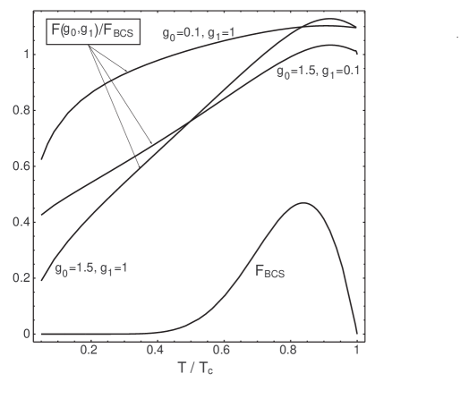
Figure 1: The temperature dependence of neutrino energy losses. Lowest curve – the function $F_{\mathrm{BCS}}$, as given by Eq. (128). Upper curves – the ratio $F/F_{\mathrm{BCS}}$ for three different combinations of Landau parameters $g_{0},g_{1}$ shown near the curves.

VIII Summary and conclusion

In this paper, we have investigated the Fermi-liquid effects in the neutrino emission at the pair recombination of thermal excitations in a superfluid crust of neutron stars. For this purpose, we have calculated the weak response functions of superfluid fermion system at finite temperatures while taking into account the particle-hole interactions near the Fermi surface. For the calculation, we used Leggett approach to strongly interacting Fermi liquid with pairing. In the case $\mathrm{q}V_{F}\ll\mathsf{\Delta}$, typical for the weak processes in the nonrelativistic baryon matter of neutron stars, we have derived the response functions valid at finite temperature and for arbitrary transferred energy $\omega\lessgtr\Delta$. Our general expressions, as given by Eqs. (55), (88), (104), and (105), naturally reproduce the well-known results Leggett , Larkin obtained for the case of small transferred energy, $\omega\ll\Delta,$ as well as the response functions obtained for arbitrary $\omega$ in the BCS approximation L08 .

In the kinematic domain $\omega>2\Delta$ and $\mathrm{q}<\omega$, we have carefully calculated the imaginary part of the response functions up to the necessary accuracy, what allows us to evaluate the neutrino energy losses caused by the pair recombination while taking into account the Fermi-liquid effects.

In the vector channel, we found that the spherical harmonic of the particle-hole interaction does not affect the imaginary parts of polarization functions in the time-like domain. The imaginary part of both the longitudinal and transverse polarization functions are proportional to $V_{F}^{4}$, and thus the particle-hole interactions are not able to increase substantially the intensity of neutrino-pair emission through the vector channel.

The imaginary part of the axial polarization is suppressed as $V_{F}^{2}$, therefore the dominating neutrino emission occurs in the axial channel. We do not support the statement of Ref. KV08 that the particle-hole interactions can be ignored [see the discussion after Eq. (33) of Ref. KV08 ). Our analytic expression (124) and numerical estimates demonstrate the important role of the Fermi liquid effects in the considered process.

IX HERE

Discarding the particle-hole interactions means that the result obtained in Ref. KV08 , as a matter of fact, corresponds to the BCS approximation. This approximation has been used before by several authors. Therefore for comparison, we consider the BCS limit of our Eq. (119) which can be obtained by putting $g_{0}=g_{1}=0$. The detailed analysis of some controversial results of different authors can be found at the end of Sec. VI.

For completeness, it is helpful to discuss additionally the case, when the quasiparticles carry an electric charge. Though the direct neutrino interaction with recombining protons is screened by the proton background LP06 , the proton quantum transitions can excite background electrons, thus inducing the neutrino-pair emission by the electron plasma. This effect has been already studied in Refs. L00 , L01 ; therefore, we only briefly revisit this problem in the light of modern theory to understand whether the plasma effects can lead to noticeable neutrino energy losses through the vector channel. For the sake of simplicity we consider a degenerate plasma consisting of nonrelativistic superfluid protons and relativistic electrons. As found in Refs. L00 , L01 , the role of the electron background, in this case, consists of the effective renormalization of the proton vector weak coupling constant, $c_{V}^{\left(p\right)}/2\rightarrow c_{V}^{\left(e\right)}$.  Thus we find that the electron background strongly increases the effective proton vector weak coupling with the neutrino field, $\left(4c_{V}^{\left(e\right)}/c_{V}^{\left(p\right)}\right)^{2}\simeq\allowbreak 576.$ However, this huge factor should not mislead the reader, because it arises only as a result of a very small proton coupling constant, $c_{V}^{\left(p\right)}\ll c_{V}^{\left(e\right)}$. Since the degenerate electron plasma can be considered in the collisionless approximation, the imaginary part of the medium polarization arises from the proton pair recombination and therefore is proportional to $V_{F}^{4}$, where $V_{F}\ll 1$ is the Fermi velocity of protons. Thus the neutrino emission through the vector channel is suppressed by a small factor $V_{F}^{4}$ and may be ignored in comparison with the dominating neutrino radiation in the axial channel, where the neutrino energy losses are suppressed as $V_{F}^{2}$.

We now return to the Fermi-liquid effects incorporated in Eq. (119). The magnitudes of the Landau parameters $g_{0},g_{1}$ are poorly known and depend on the baryon density. By modern estimates Sapershtein , Rodin , these could be of the order of unity. Thus the Fermi-liquid effects can notably modify the emissivity dependence on the temperature and the matter density as compared to that found in the BCS approximation. This, however, cannot change the main conclusion that the dominating contribution to the neutron and proton emissivity comes from the axial channel of weak interactions L08 . This means that the neutrino energy losses are to be suppressed as compared to that of Ref. FRS76 by a factor of $V_{F}^{2}$. This could serve by a natural explanation of the observed superburst ignition discussed in the Introduction.

References

• (1) E. Flowers, M. Ruderman, and P. Sutherland, Astrophys. J., 205 541 (1976).
• (2) L. B. Leinson and A. Pérez, Phys. Lett. B638 114 (2006).
• (3) A. Sedrakian, H. Müther, and P. Schuck,Phys. Rev. C 76, 055805 (2007).
• (4) L. B. Leinson, Phys. Rev. C 78, 015502 (2008).
• (5) E. E. Kolomeitsev, and D. N. Voskresensky, Phys. Rev. C 77, 065808 (2008).
• (6) A. W. Steiner, and S. Reddy, Phys. Rev. C 79, 015802 (2009).
• (7) A. Cumming, J. Macbeth, J. J. M. I. Zand & D. Page, Astrophys. J., 646, 429 (2006).
• (8) S. Gupta, E. F. Brown, H. Schatz, P. Moller, and K.-L. Kratz, Astrophys. J. 662, 1118, (2007).
• (9) A. J. Leggett, Phys. Rev. 140, 1869 (1965); A. J. Leggett, Phys. Rev. 147, 119 (1966).
• (10) A. I. Larkin and A. B. Migdal, Sov. Phys. JETP 17, 1146 (1963).
• (11) A.D. Kaminker, P. Haensel, D.G. Yakovlev, Astron. Astrophys 345, L14 (1999).
• (12) L. B. Leinson, Phys. Lett. B 473, 318 (2000).
• (13) L. B. Leinson, Nucl. Phys. A 687, 489 (2001).
• (14) A. A. Abrikosov, L. P. Gorkov, I. E. Dzyaloshinkski, Methods of Quantum Field Theory in Statistical Physics, (Dover, New York, 1975).
• (15) A. B. Migdal, Theory of Finite Fermi Systems and Applications to Atomic Nuclei  (Interscience, London, 1967).
• (16) N. N. Bogoliubov, Soviet Phys. Uspekhi 67 236 (1959) [Uspekhi Fiz. Nauk 67, 549 (1959)].
• (17) P. Jaikumar, M. Prakash, Phys.Lett. B 516, 345 (2001).
• (18) E. E. Sapershtein and S. V. Tolokonnikov, JETP Lett. 68, 553 (1998); S. A. Fayans and D. Zawischa, Phys. Lett. B 383, 19 (1996).
• (19) V. A. Rodin, A. Faessler, F. Simkovic, and P. Vogel, Nucl. Phys. A 766, 107 (2006); A 793, 213(E) (2007).