Quantum synchronization and entanglement of two qubits
coupled to a driven dissipative resonator

Abstract

Using method of quantum trajectories we study the behavior of two identical or different superconducting qubits coupled to a quantum dissipative driven resonator. Above a critical coupling strength the qubit rotations become synchronized with the driving field phase and their evolution becomes entangled even if two qubits may significantly differ from one another. Such entangled qubits can radiate entangled photons that opens new opportunities for entangled wireless communication in a microwave range.

Recently, an impressive experimental progress has been reached in realization of a strong coupling regime of superconducting qubits with a microwave resonator wallraff ; majer ; wallraff1 ; wallraff2 ; wallraff3 . The spectroscopy of exchange of one to few microwave photons with one wallraff ; wallraff1 , two majer ; wallraff2 and even three wallraff3 superconducting qubits has been demonstrated to be in agreement with the theoretical predictions of the Jaynes-Cummings and Tavis-Cummings models jaynes ; tavis ; scully even if certain nonlinear corrections have been visible. Thus the ideas of atomic physics and quantum optics find their promising implementations with superconducting macroscopic circuits leading also to achievement of single artificial-atom lasing in a microwave range astafiev .

In comparison to quantum optics models jaynes ; tavis ; scully a new interesting element of superconducting qubits is the dissipative nature of coupled resonator which opens new perspectives for quantum measurements korotkov . At the same time in the strongly coupled regime the driven dissipative resonator becomes effectively nonlinear due to interaction with a qubit that leads to a number of interesting properties shnirman1 ; gambetta ; zhirov2008 . Among them is synchronization of qubit with a driven resonator phase zhirov2008 corresponding to a single artificial-atom lasing realized experimentally in astafiev . The synchronization phenomenon has broad manifestations and applications in physics, engineering, social life and other sciences pikovsky but in the above case we have a striking example of quantum synchronization of a purely quantum qubit with a driven resonator having a semiclassical number of a few tens of photons zhirov2008 . This interesting phenomenon appears above a certain critical coupling threshold zhirov2008 and its investigation is now in progress shnirman2 .

Due to the experimental progress with two and three qubits majer ; wallraff2 ; wallraff3 it is especially interesting to study the case of two qubits where an interplay of quantum synchronization and entanglement opens a new field of interesting questions. The properties of entanglement for two atoms (qubits) coupled to photons in a resonator has been studied recently in the frame of Tavis-Cummings model within the rotating wave approximation (RWA) deutsch ; solano . Compared to them we are interested in the case of dissipative driven resonator strongly coupled to qubits where RWA is not necessarily valid and where the effects of quantum synchronization between qubits and the resonator is of primary importance. In addition we consider also the case of different qubits which is rather unusual for atoms but is very natural for superconducting qubits.

In absence of dissipation the whole system is described by the Hamiltonian

$$\hat{H}=\hbar\omega_{0}(\hat{n}+1/2)+\hbar\Omega_{1}\sigma^{(1)}_{z}/2+\hbar\Omega_{2}\sigma^{(2)}_{z}/2$$ (1)

$$+g\hbar\omega_{0}(\sigma^{(1)}_{x}+\sigma^{(2)}_{x})(\hat{a}+\hat{a}^{+})+f\cos\omega t\cdot(\hat{a}+\hat{a}^{+})$$

where the first three terms represent photons in a resonator and two qubits, $g$-term gives the coupling between qubits and photons and the last term is the driving of resonator. In presence of dissipation the resonator dissipation rate is $\lambda$ and its quality factor is assumed to be $Q=\omega_{0}/\lambda\sim 100$. The decay rate of qubits is supposed to be zero corresponding to a reachable experimental situation wallraff ; majer ; wallraff1 ; wallraff2 ; wallraff3 where their decay rate is much smaller than $\lambda$. The driving force amplitude is expressed as $f=\hbar\lambda\sqrt{n_{p}}$ where $n_{p}$ is a number of photons in a resonator at the resonance $\omega=\omega_{0}$ when $g=0$. The whole dissipative system is described by the master equation for the density matrix $\hat{\rho}$ which has the standard form weiss :

$$\dot{\hat{\rho}}=-\frac{i}{\hbar}[\hat{H},\hat{\rho}]+\lambda(\hat{a}\hat{\rho}\hat{a}^{{\dagger}}-\hat{a}^{{\dagger}}\hat{a}\hat{\rho}/2-\hat{\rho}\hat{a}^{{\dagger}}\hat{a}/2).$$ (2)

The numerical simulations are done by the method of quantum trajectories percival with the numerical parameters and techniques described in zhirov2008 .

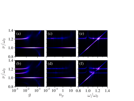
Figure 1: (Color online) Spectral density $S(\nu)$ of two driven qubits as a function of system parameters for identical $\Omega_{1}/\omega_{0}=\Omega_{2}/\omega_{0}=1.2$ (top row) and different $\Omega_{1}/\omega_{0}=1.1$, $\Omega_{2}/\omega_{0}=1.2$ (bottom row) qubits: (a,b) $n_{p}=15$, $\omega/\omega_{0}=1$; (c,d) $g=0.04$, $\omega/\omega_{0}=1$; (e,f) $n_{p}=15$, $g=0.04$. Here and below $\lambda/\omega_{0}=0.02$.

To analyze the system properties we determine the spectral density of driven qubits defined as $S(\nu)=\left|\int dt\exp\{-i\nu t\}{\rm Tr}(\hat{\rho}(\sigma^{(1)}_{x}+\sigma^{(2)}_{x})/2)\right|^{2}$. Its dependence on system parameters for identical and different qubits is shown in Fig. 1. At small couplings $g$ the spectrum of qubits $S(\nu)$ shows the lines at the internal qubit frequencies $\Omega_{1,2}$ but above a certain critical coupling strength $g>g_{c}$ the quantum synchronization of qubits with the driven resonator takes place and the unperturbed spectral lines are replaced by one dominant spectral line at the driving frequency with $\nu=\omega$ (Fig. 1a,b). A similar phenomenon takes place for $g>g_{c}(f)$ when the strength of resonator driving $f\propto\sqrt{n_{p}}$ is increased (Fig. 1c,d). Indeed, with the growth of $n_{p}$ the number of photons in the resonator increases that leads to a stronger coupling between photons and qubits and eventual synchronization. The synchronization of qubits with the resonator is also clearly seen from Fig. 1e,f, where the spectral line of $S(\nu)$ follows firmly the variation of driving frequency $\omega$. The striking feature of Fig. 1 is that even rather different qubits with significant frequency detunings $|\Omega_{1,2}-\omega_{0}|\gg\lambda$ become synchronized due to their coupling with the resonator getting the same lasing frequency $\nu\approx\omega$.

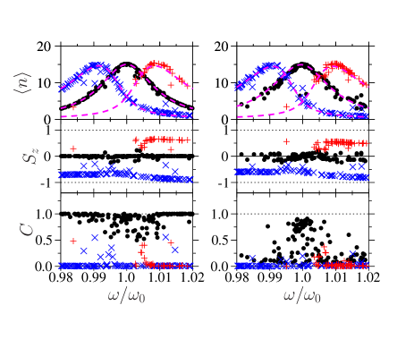
Figure 2: (Color online) The average quantities of number of photons in the resonator $<n>$ (top), total spin polarization $S_{z}$ (middle), and the concurrence of two qubits $C$ (bottom) vs. the driving frequency $\omega$. Left: identical qubits with $\Omega_{1}/\omega_{0}=\Omega_{2}/\omega_{0}=1.2$, right: different qubits with $\Omega_{1}/\omega_{0}=1.1$, $\Omega_{2}/\omega_{0}=1.2$. Other parameters are $\lambda/\omega_{0}=0.02$, $n_{p}=15$, $g=0.04$. Symbols mark the values of the total spin $S_{z}$: $S_{z}>0.2$ (red/gray $+$), $|S_{z}|\leq 0.2$ (black dots), $S_{z}<-0.2$ (blue/black $\times$). Dashed curves on top panels show the resonance dependence $n_{S_{z}}(\omega)$ (see text) with the resonance shift $\Delta\omega_{S_{z}}=1.35S_{z}g\omega_{0}\sqrt{(1-<S_{z}>^{2})/(n_{S_{z}}+1)}$.

For a better understanding of this phenomenon we analyze the dependence of the average number of photons in the resonator $<n>$ on driving frequency $\omega$ (see Fig. 2, top panels). It has three pronounced maxima which up to quantum fluctuations correspond to three values of the total spin component $S_{z}={\rm Tr}(\hat{\rho}(\sigma^{(1)}_{z}+\sigma^{(2)}_{z})/2)$ being close to the values $S_{z}=-1,0,1$ with the total spin $S=1$ (triplet state) as it is clearly seen from the data shown in the middle panels of Fig. 2. The whole dependence of $<n>$ on $\omega$ is well fitted by the resonance curves $n_{S_{z}}=n_{p}\lambda^{2}/[4(\omega-\omega_{0}-\Delta\omega_{S_{z}})^{2}+\lambda^{2}]$ where the frequency shift $\Delta\omega_{S_{z}}$ appears due to the effective Rabi frequency $\Omega_{R}$ which gives oscillations between the resonant states. The value of $\Omega_{R}$ is induced by the coupling between qubits and photons in Eq.(1) jaynes ; tavis ; scully and can be approximated obtained as an average value of coupling that gives $\Omega_{R}=2aS_{z}g\omega_{0}\sqrt{(1-<S_{z}>^{2})(n_{S_{z}}+1)}\approx 2S_{z}a\Omega_{R0}$ with $\Omega_{R0}=g\omega_{0}\sqrt{n_{S_{z}}+1}$. This gives the frequency shift $\Delta\omega_{S_{z}}=d\Omega_{R}/dn_{S_{z}}$ which determines the resonant dependence $n_{S_{z}}(\omega)$ in a self consistent way. Such a theory gives a good description of numerical data as it is shown in Fig. 2 (top panel) where the corresponding values of $<S_{z}>$ are taken from the middle panel. The numerical coefficient $a$ smoothly varies between $1.14$ and $1.57$ for $0.01\leq g\leq 0.06$. This resonance dependence is similar to the one qubit case discussed in zhirov2008 but the effects of quantum fluctuations are larger due to mutual effective coupling between qubits via the dissipative resonator. On the basis of these estimates it is natural to assume that the quantum synchronization of a qubit with a driving phase takes place under the condition that the detuning is smaller than the typical value of Rabi frequency

$$\left|\Omega_{1,2}-\omega\right|<\Omega_{R0}=g\omega_{0}\sqrt{n_{S_{z}}+1}\approx g\omega_{0}\sqrt{n_{p}+1}.$$ (3)

This criterion assumes a semiclassical nature of photon field with the number of photons $n_{p}>1$. Its structure is similar to the classical expression for the synchronization tongue which is proportional to the driving amplitude being independent of dissipation rate pikovsky . The relation (3) determines the border for quantum synchronization $g_{c}\approx\left|\Omega_{1,2}-\omega\right|/\omega_{0}\sqrt{n_{p}+1}$.

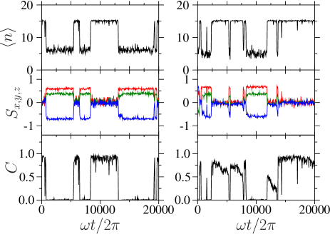
Figure 3: (Color online) Time evolution of system quantities: average photon number $<n>$ (top); components of total spin polarization $S_{x,y,z}$ (middle) where $x,y,z$-components correspond to red, green, blue colors (curves from top to bottom at $\omega t/2\pi=1.5\times 10^{4}$ (left) and $\omega t/2\pi=10^{4}$ (right)); concurrence $C$ (bottom). Left: two identical qubits with $\Omega_{1,2}/\omega_{0}=1.2$, right: two different qubits with $\Omega_{1}/\omega_{0}=1.1$ and $\Omega_{1}/\omega_{0}=1.2$. Data are shown at stroboscopic moments of time with driving phase $\varphi=\omega t\;({\rm mod}\;2\pi)=0$, Here $\omega/\omega_{0}=1$, other parameters are as in Fig. 2.

The entanglement between qubits is characterized by concurrence $C$ (see e.g. the definition in deutsch ). Its dependence on $\omega$ is shown in the bottom panels of Fig. 2. It is striking that the concurrence $C$ can be close to unity not only for identical qubits but also for different qubits. Qualitatively, this happens due to synchronization of qubits induced by the resonator driving which makes them “quasi-identical” and allows to create the entangled state with $S_{z}=0$.

To understand the properties of the system in a better way we show the time evolution of its characteristics along a typical quantum trajectory in Fig. 3. Average number of photons in the resonator $<n>$ shows tunneling transitions between two metastable states induced by quantum fluctuations (top panels). There are no transitions to the third metastable state, seeing in Fig. 2 with three resonant curves, but we had them on longer times or for other realizations of quantum trajectories (see also Fig. 4). The life time inside each metastable state is of the order of thousands of driving periods and the change of $<n>$ is macroscopically large (about a ten of photons). The transition leads also to a change of total spin polarization components $S_{x,y,z}={\rm Tr}(\hat{\rho}(\sigma^{(1)}_{x,y,z}+\sigma^{(2)}_{x,y,z})/2)$ (middle panels). It takes place on a relatively short time scale $\sim 1/\lambda$. The transition also generates emergence or death of concurrence $C$ (or entanglement) which happens on the same time scale $1/\lambda$ (bottom panels). Naturally, $C$ is maximal when $S_{x}\approx 0$. Remarkably, during long time intervals $C$ remains to be close to its maximal value $C=1$ even for the case of different qubits. We attribute this phenomenon to synchronization of two qubits by driven resonator.

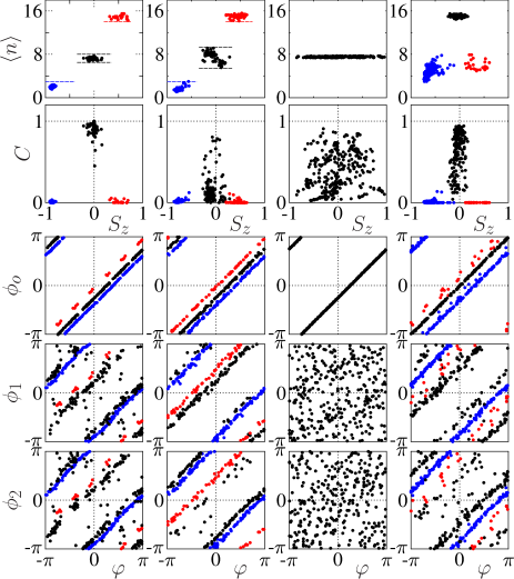
Figure 4: (Color online) Rows from top to bottom: average photon number $\left\langle n\right\rangle$ vs. $S_{z}$; concurrence $C$ vs. $S_{z}$; resonator phase $\phi_{o}$, and qubits phases $\phi_{1,2}$ vs. the driving force phase $\varphi$. Columns from left to right: (i) two identical qubits with $\Omega_{1,2}/\omega_{0}=1.2$, $g=0.04$, (ii-iii) two different qubits, with $\Omega_{1}/\omega_{0}=1.1$, $\Omega_{2}/\omega_{0}=1.2$, $g=0.04$ and $g=0.001$, all tree columns correspond to driving frequency $\omega/\omega_{0}=1.01$. The last column (iv) shows data for two different qubits with $\Omega_{1}/\omega_{0}=1.1$, $\Omega_{2}/\omega_{0}=1.2$, $g=0.04$ but the driving frequency $\omega/\omega_{0}=1$ (cf. (ii)). Colors of points are explained in the text. Other parameters of simulations are: $\lambda/\omega_{0}=0.02$, $n_{p}=15$.

To display and characterize this phenomenon in more detail we determine the phases of oscillator and qubits via relations $\phi_{0}=\arctan({\rm Im}\langle\hat{a}\rangle/{\rm Re}\langle\hat{a}\rangle)$, $\phi_{1,2}=\arctan(<s^{(1,2)}_{x}>/<s^{(1,2)}_{y}>)$ respectively. The variation of these phases with the driving phase $\varphi=\omega t\;({\rm mod}\;2\pi)$ is shown in Fig. 4 for different values of system parameters corresponding to columns (i, ii, iii, iv). For identical qubits (column (i)) the numerical data obtained along one long quantum trajectory form three well defined groups of points in the plane of $<n>$ and $S_{z}$ (data are taken at stroboscopic moments of time $t$ with a certain frequency comparable but incommensurate with $\omega$ to sweep all phases $\varphi$). It is convenient to mark these groups by three different colors corresponding to small (blue or dark grey), medium (black) and large (red or light grey) values of $<n>$ (the groups are also marked by horizontal lines). Such a classification shows that three groups have not only distinct values of $<n>$ but also three distinct locations in concurrence $C$ and spin $S_{z}$. Also these groups show three lines in the phase plane for oscillator $(\phi_{0},\varphi)$ and for each qubit $(\phi_{1,2},\varphi)$. Of course, due to quantum fluctuations there are certain fluctuations for qubit phases but the linear dependence between phases is seen very clearly, thus showing the quantum synchronization of system phases with the driving phase $\varphi$. Physically, the three groups correspond to the three triplet states of total spin $S=1$. Indeed, for identical qubits the states with total spin values $S=1$ and $S=0$ are decoupled and the dynamics of $S=0$ state is trivial (see Eq. (1)). For different qubits (columns (ii), (iv)) the quantum synchronization between phases is also clearly seen even if two qubits have rather different frequency detunings. For the case (ii) the concurrence is smaller compared to the case of identical qubits (i) but by a change of driving frequency $\omega$ it can be increased (see the case (iv)) to the values as high as for identical qubits in (i). We note that for different qubits (e.g. for (ii)) there is a visible splitting of the middle group of black points in $(<n>,S_{z})$ plane which corresponds to states with mixed components of total spin $S=1$ and $S=0$: indeed, for different qubits the coupling between the states $S=1$ and $S=0$ is nonzero and such transitions can take place (however, on the phase planes the splitting of black points is too weak to be seen in presence of quantum fluctuations). Of course, the numerical data show the presence of quantum fluctuations around straight lines in the phase planes. Nevertheless, this regime of quantum synchronization at $g>g_{c}$ is qualitatively different from the regime below the synchronization border $g<g_{c}$ where the points are completely scattered over the whole phase plane (column (iii)). In this regime (iii) the qubits rotate independently from the resonator which stays at fixed number of photons. In contrast, for $g>g_{c}$ two qubits move in quantum synchrony during a large number of oscillations being entangled. A single superconducting qubit lasing has been already achieved in experiments astafiev . Our theoretical studies show that such two qubits, which in practice are always non-identical, can be made entangled and produce lasing in synchrony with each other. Being entangled such qubits can radiate entangled photons in a microwave range. Therefore, the experiments similar to astafiev but with two single-atoms lasing would be of great interest for entangled microwave photons generation.

In conclusion, our numerical simulations show that even two different superconducting qubits can move in quantum synchrony induced by coupling to a driven dissipative resonator, which can make them entangled. Such entangled qubits can radiate entangled microwave photons that opens interesting opportunities for wireless entangled communication in a microwave domain.

The work is funded by EC project EuroSQIP and RAS grant ”Fundamental problems of nonlinear dynamics”.

References

- (1) A. Wallraff, D. I. Schuster, A. Blais, L. Frunzio, R. S. Huang, J. Majer, S. Kumar, S. M. Girvin and R. J. Schoelkopf, Nature 431, 162 (2004).
- (2) J. Majer, J. M. Chow, J. M. Gambetta, J. Koch, B. R. Johnson, J. A. Schreier, L. Frunzio, D. I. Schuster, A. A. Houck, A. Wallraff, A. Blais, M. H. Devoret, S. M. Girvin and R. J. Schoelkopf, Nature 449, 443 (2007).
- (3) J. M. Fink, M. Göppl, M. Baur, R. Bianchetti, P. J. Leek, A. Blais and A. Wallraff, Nature 454, 315 (2008).
- (4) S. Filipp, P. Maurer, P. J. Leek, M. Baur, R. Bianchetti, J. M. Fink, M. Göppl, L. Steffen, J. M. Gambetta, A. Blais and A. Wallraff, arXiv:0812.2485[cond-mat] (2008).
- (5) J. M. Fink, R. Bianchetti, M. Baur, M. Goeppl, L. Steffen, S. Filipp, P. J. Leek, A. Blais and A. Wallraff, arXiv:0812.2651[cond-mat] (2008).
- (6) E. T. Jaynes and F. W. Cummings, Proc. IEEE 51, 89 (1963).
- (7) M. Tavis and F. W. Cummings, Phys. Rev. 170, 379 (1968).
- (8) M.O. Scully and M.S. Zubairy, Quantum optics, Cambridge Univ. Press, Cambridge (1997).
- (9) O. Astafiev, K. Inomata, A. O. Niskanen, T. Yamamoto, Yu. A. Pashkin, Y. Nakamura and J. S. Tsai, Nature 449, 588 (2007).
- (10) A.N. Korotkov, Phys. Rev. B 60, 5737 (1999); ibid. 67, 235408 (2003); A.N. Korotkov and D.V. Averin, ibid. 64, 165310 (2001).
- (11) J. Hauss, A. Fedorov, C. Hutter, A. Shnirman, and G. Schön, Phys. Rev. Lett. 100, 037003 (2008).
- (12) J. Gambetta, A. Blais, M. Boissonneault, A. A. Houck, D. I. Schuster and S. M. Girvin, Phys. Rev. A 77, 012112 (2008).
- (13) O.V.Zhirov and D.L.Shepelyansky, Phys. Rev. Lett. 100, 014101 (2008).
- (14) A. Pikovsky, M. Rosenblum, and J. Kurths, Synchronization: A Universal Concept in Nonlinear Sciences, Cambridge Univ. Press (2001).
- (15) S. André, V. Brosco, A. Shnirman, and G. Schön, arXiv:0807.4607v2 (2008).
- (16) T.E. Tessier, I. H. Deutsch, A. Delgado, and I. Fuentes-Guridi, Phys. Rev. A 68, 062316 (2003).
- (17) A. Retzker, E. Solano, and B. Reznik, Phys. Rev. A 75, 022312 (2007).
- (18) U. Weiss, Dissipative quantum mechanics. World Sci., Singapore (1999).
- (19) T.A. Brun, I.C. Percival, and R. Schack, J. Phys. A 29, 2077 (1996); T.A. Brun, Am. J. Phys. 70, 719 (2002).