Spin-fluctuation drag thermopower of nearly ferromagnetic metals

Abstract

We investigate theoretically the Seebeck effect in materials close to a ferromagnetic quantum critical point to explain anomalous behaviour at low temperatures. It is found that the main effect of spin fluctuations is to enhance the coefficient of the leading $T$-linear term, and a quantum critical behaviour characterized by a spin-fluctuation temperature appears in the temperature dependence of correction terms as in the specific heat.

1 Introduction

Experiments on clean materials near ferromagnetic quantum critical point (QCP) have revealed unusual properties, including non Fermi liquid transport and unconventional superconductivity.[1, 2] The effects caused by quantum critical dynamics of spin fluctuations on the specific heat coefficient, the spin susceptibility, the resistivity, and so on, have been elucidated analytically at low temperatures.[3, 4, 5, 6, 7] In most of such theoretical analyses made so far, critical spin fluctuations are regarded to stay in thermal equilibrium. On the other hand, one may conceive of its inequilibrium counterpart of anomalous behaviours as well, which would be of fundamental interest too and should be paid due attention theoretically. As a representative of such phenomena, there are observations suggesting spin-fluctuation (or paramagnon) drag thermopower. In the Seebeck coefficient $S(T)$ of ${\rm UAl_{2}}$, for example, there have remained a structure at low temperature, which is observed experimentally,[8, 9] but left unexplained theoretically.[10, 11] Among others, the most typical clear-cut experimental evidence would be those reported by Gratz $et$ $al$.,[12, 13, 14] where the pronounced low-temperature minimum in $S(T)$ of strong paramagnet $\rm RCo_{2}$ (R$=$Sc, Y and Lu) was attributed to the paramagnon drag effect. Recently, Matsuoka $et$ $al$.[15] found a similar structure for $\rm AFe_{4}Sb_{12}$ (A$=$Ca, Sr and Ba). In effect, Takabatake $et$ $al$.[16] made it clear that the anomaly in $S(T)$ is indeed caused by the ferromagnetic spin fluctuations prevalent in the materials by showing that those structure is completely suppressed by applying a uniform magnetic field. In contrast with the accumulating experimental evidence, there seems no theory to compare with the experiments available so far, with the exception of a brief account on a qualitative effect expected for localized spin fluctuations around impurity sites of alloys.[17] In this paper, we discuss an effect of uniform spin fluctuations in a translationally invariant system, and intend to provide a more solid footing on which to discuss the phenomenon.

In section 2, we give an outline of a two-band model, which we adopt as a relevant model, along with approximations and assumptions conventionally made. In section 3, we introduce a function $\Phi_{k}^{d}$ to represent inequilibrium displacement of spin fluctuations. In section 4, we discuss that the leading effect of spin fluctuations appears on the $T$-linear term of $S(T)$. In effect, in section 4.2, we discuss that the leading term contribution follows a universal relation to the specific heat, that is, $q\equiv eS/C\simeq\pm 1$ revealed by Behnia $et$ $al$.[18] In the higher order terms, we have to consider not only a critical effect originating from equilibrium quantities, but also a genuinely non-equilibrium effect which has not been investigated before. In section 5, we investigate the latter contributions to find a characteristic temperature dependence, and the results are summarized in the last subsection 5.4. In section 6, we discuss the results and comparison is made with experiment.

2 Model

Let us introduce a two-band paramagnon model, which is conventionally employed to explain an enhanced resistivity of transition metals at low temperature.[5, 19, 20] The model has been applied successfully to explain, e.g., a saturation behaviour at elevated temperatures by taking into account a proper temperature dependence of spin susceptibility.[21, 22]

The model is comprised of two types of electrons, i.e., wide-band conduction electrons and narrow-band itinerant electrons on the border of ferromagnetism. We denote the former as the $s$ electron and the latter as the $d$ electrons, representatively. The Hamiltonian consists of three parts,

$$H=H_{s}+H_{sd}+H_{d}.$$

The free Hamiltonian of the $s$ electron is given by

$$H_{s}=\sum_{k\sigma}\varepsilon_{s}(k)c^{\dagger}_{k\sigma}c_{k\sigma},$$

where $c^{\dagger}_{k\sigma}$ and $c_{k\sigma}$ are the creation and annihilation operators for the electron with momentum $k$ and spin $\sigma$. For simplicity, it is often assumed that the $s$ electrons make a parabolic band with mass $m_{s}$, i.e.,

$$\varepsilon_{s}(k)=\frac{k^{2}}{2m_{s}}.$$ (1)

At each site $i$, they are scattered by the spin ${\bi S}_{i}$ of the $d$ electron at the same site through the Kondo $s$-$d$ coupling,

$$H_{sd}=J\sum_{i}{\bi s}_{i}\cdot{\bi S}_{i},$$ (2)

where $J$ denotes a coupling constant, and ${\bi s}_{i}=\frac{1}{2}\sum_{\sigma\sigma^{\prime}}c^{\dagger}_{i\sigma}{\bi\tau}_{\sigma\sigma^{\prime}}c_{i\sigma}$ is the spin of the $s$ electron at the site $i$ expressed in terms of the Pauli matrix vector ${\bi\tau}_{\sigma\sigma^{\prime}}$. Similarly, the $d$ electron spin at the site $i$ is given by ${\bi S}_{i}=\frac{1}{2}\sum_{\sigma\sigma^{\prime}}d^{\dagger}_{i\sigma}{\bi\tau}_{\sigma\sigma^{\prime}}d_{i\sigma}$ in terms of the creation and annihilation operators $d^{\dagger}_{i\sigma}$ and $d_{i\sigma}$ for the $d$ electron. Spin dynamics of the $d$ electrons is described by the Hubbard Hamiltonian,

$$H_{d}=\sum_{k\sigma}\varepsilon_{d}(k)d^{\dagger}_{k\sigma}d_{k\sigma}+U\sum_{i}n_{i\uparrow}n_{i\downarrow},$$ (3)

where $n_{i\sigma}=d^{\dagger}_{i\sigma}d_{i\sigma}$ $(\sigma=\uparrow,\downarrow)$ is the number operator of the $d$ electron at the site $i$. The on-site repulsion $U$ is fixed such that the $d$ band is nearly ferromagnetic. To make analytical evaluation feasible, it is often assumed further that the $d$ electrons are also parabolic with a different mass $m_{d}$ heavier than $m_{s}$, i.e.,

$$\varepsilon_{d}(k)=\frac{k^{2}}{2m_{d}},$$ (4)

and $m_{d}\gg m_{s}$. The latter inequality is regarded as the basic ingredient of the model. Hence the $d$ electrons act as heavy and fluctuating scatterers against the $s$ electrons through the coupling of (2). In effect, this is taken into account as the second order effect with respect to the coupling $J$, i.e., through the Born approximation.[19] Then, the $d$ electron comes into play through the (transverse) spin susceptibility $\chi(q,\omega)$. In the random phase approximation, it is given by

$$\chi(q,\omega)=\frac{\chi_{0}(q,\omega)}{1-U\chi_{0}(q,\omega)},$$ (5)

where

$$\chi_{0}(q,\omega)=\sum_{k}\frac{f^{0}_{k}-f^{0}_{k+q}}{\varepsilon_{d}(k+q)-\varepsilon_{d}(k)-\omega-{\rm i}\delta}.$$ (6)

Here, $f_{k}^{0}\equiv f^{0}(\varepsilon_{d}(k))=1/({\rm e}^{(\varepsilon_{d}(k)-\mu)/T}+1)$ is the Fermi distribution function, and $\delta$ is a positive infinitesimal. To investigate critical properties at low temperatures,[23] (6) is expanded for small $q$ and $\omega/q$ as

$$\chi_{0}(q,\omega)=\rho_{F,d}\left(1-\frac{1}{12}\bar{q}^{2}+{\rm i}\frac{\pi}{4}\frac{\bar{\omega}}{\bar{q}}\right),$$ (7)

for $\bar{\omega}<2\bar{q}$, where $\bar{q}=q/k_{F,d}$ and $\bar{\omega}=\omega/\varepsilon_{F,d}$ are the momentum and energy normalized by the Fermi momentum $k_{F,d}$ and the Fermi energy $\varepsilon_{F,d}$ of the $d$ electron. $\rho_{F,d}=m_{d}k_{F,d}/2\pi^{2}$ is the density of states (DOS) at the Fermi level of the $d$ electron per spin. Substituting (7) into (5), we obtain

$$\chi(q,\omega)=\frac{\rho_{F,d}}{K_{0}^{2}+\frac{\bar{U}}{12}\bar{q}^{2}-{\rm i}\frac{\pi\bar{U}}{4}\frac{\bar{\omega}}{\bar{q}}},$$ (8)

for $\bar{\omega}<2\bar{q}$, where $\bar{U}=\rho_{F,d}U$, and $K_{0}^{2}=1-\bar{U}(\ll 1)$ represents the distance to the QCP.

The intrinsic transition probability ${\cal Q}_{k,q}^{k+q}$ that an $s$ electron with momentum $k$ is scattered to $k+q$ by absorbing a spin fluctuation with $q$ and $\omega$ via the coupling in (2) is given by

$${\cal Q}_{k,q}^{k+q}(\omega)=\frac{3J^{2}}{4}S(q,\omega),$$ (9)

where $S(q,\omega)$ denotes the Fourier transform of the spin density correlation function, which is related to the dynamical susceptibility by the fluctuation dissipation theorem.[23]

$$S(q,\omega)=\frac{2}{1-{\rm e}^{-\omega/T}}{\rm Im}\chi(q,\omega).$$ (10)

The equilibrium transition rate is given by

$${\cal P}_{k,q}^{k+q}=\int{\rm d}\omega(1-f^{0}(\varepsilon_{s}({k+q})))f^{0}(\varepsilon_{s}(k))n^{0}(\omega){\cal Q}_{k,q}^{k+q}(\omega)\delta(\omega+\varepsilon_{s}(k)-\varepsilon_{s}({k+q})),$$ (11)

where $f^{0}(\varepsilon_{s}(k))$ is the Fermi factor for the $s$ electron, and $n^{0}(\omega)=1/({\rm e}^{\omega/T}-1)$ is the Bose function. With this ${\cal P}_{k,q}^{k+q}$, transport coefficients are derived by following the formal transport theory of Ziman[24] (cf. A). Transport properties of the $s$ electrons in an electric field ${\bi E}$ and a gradient of temperature $\nabla T$ are described by the Boltzmann transport equation,

$$-{\bi v}_{s}(k)\cdot\nabla T\frac{\partial f^{0}(\varepsilon_{s}(k))}{\partial T}-e{\bi v}_{s}(k)\cdot{\bi E}\frac{\partial f^{0}(\varepsilon_{s}(k))}{\partial\varepsilon_{s}(k)}=-\dot{f}_{k},$$ (12)

where ${\bi v}_{s}(k)=\nabla_{k}\varepsilon_{s}(k)$ is the velocity of the $s$ electron, and $e(<0)$ is the electronic charge. The right-hand side in (12) is the collision integral for the $s$ electron.

To linearize the transport equation for the conduction electrons, a function $\Phi_{k}^{s}$ to represent the displacement of the distribution function $f(\varepsilon_{s}(k))$ from the equilibrium one $f^{0}(\varepsilon_{s}(k))$ is introduced, i.e., by

$$f(\varepsilon_{s}(k))=f^{0}(\varepsilon_{s}(k))-\frac{\partial f^{0}(\varepsilon_{s}(k))}{\partial\varepsilon_{s}(k)}\Phi_{k}^{s}.$$ (13)

On the contrary, the $d$ electrons are commonly assumed to stay in equilibrium, despite the applied fields. Then, for the collision integral in (12), we obtain

$$\dot{f}_{k}=-\frac{1}{T}\sum_{q}\left(\Phi_{k}^{s}-\Phi_{k+q}^{s}\right){\cal P}_{k,q}^{k+q}.$$ (14)

For definiteness, let the fields ${\bi E}$ and $\nabla T$ be in the direction parallel to a unit vector ${\bi u}$. For the isotropic model, the magnitudes of the electric and heat currents due to the $s$ electrons are given by

$${J}_{s}[\Phi^{s}]=2e\sum_{k}{\bi u}\cdot{\bi v}_{s}(k)\left(-\frac{\partial f^{0}(\varepsilon_{s}(k))}{\partial\varepsilon_{s}(k)}\right)\Phi_{k}^{s},$$ (15)

and

$${U}_{s}[\Phi^{s}]=2\sum_{k}{\bi u}\cdot{\bi v}_{s}(k)(\varepsilon_{s}(k)-\mu)\left(-\frac{\partial f^{0}(\varepsilon_{s}(k))}{\partial\varepsilon_{s}(k)}\right)\Phi_{k}^{s}.$$ (16)

The factor 2 in front of the $k$ sum accounts for the two spin components. As noted below (13), it is conventionally assumed that the corresponding currents due to the $d$ electrons are neglected against the $s$ electron currents.

To obtain a solution $\Phi_{k}^{s}$, one may set $\Phi_{k}^{s}=\tau{\bi u}\cdot{\bi v}_{s}(k)$, while the constant $\tau$ is fixed by the equation. Consequently, for the electric resistivity $R=R_{0}(T)$ and the diffusion thermopower coefficient $S=S_{0}^{s}(T)$, we obtain

$$R_{0}(T)=\frac{P_{ss}}{({J_{s}}[\Phi^{s}])^{2}},$$ (17)

and

$$S_{0}^{s}(T)=\frac{1}{T}\frac{{U_{s}}[\Phi^{s}]}{{J_{s}}[\Phi^{s}]},$$ (18)

where

$$P_{ss}=\frac{1}{T}\sum_{k,q}{\cal P}^{k+q}_{kq}\left(\Phi_{k}^{s}-\Phi_{k+q}^{s}\right)^{2}.$$ (19)

The ordinary diffusion thermopower in (18) is linear in $T$ at low temperature, and is often expressed as

$$S_{0}^{s}(T)=\frac{\pi^{2}T}{3e}\frac{\partial\log\sigma_{s}(\varepsilon_{F,s})}{\partial\varepsilon},$$

in terms of the spectral conductivity $\sigma_{s}(\varepsilon)$ of the conduction electron.

3 Spin-fluctuation drag

As remarked above, the $d$ electrons are customarily assumed to stay in equilibrium regardless of the applied fields. To generalize the above framework to describe spin fluctuations with a shifted distribution theoretically, let us consider a bare dragged susceptibility $\chi^{q_{0}}_{0}(q,\omega)$, which is obtained by shifting uniformly the equilibrium bare susceptibility $\chi_{0}(q,\omega)$ in (6) by a small but finite amount ${\bi q}_{0}$ in momentum space. Similarly, we may define $\chi^{q_{0}}(q,\omega)$ for the full susceptibility $\chi(q,\omega)$ as well. Hence, $\chi^{q_{0}}(q,\omega)$ is strongly peaked at ${\bi q}={\bi q}_{0}$.

First we derive a simple relation between $\chi^{q_{0}}_{0}(q,\omega)$ and $\chi_{0}(q,\omega)$. According to (5), we will obtain a similar relation for the full susceptibility. For the derivation, we introduce a shifted energy of the $d$ electron,

$$\varepsilon_{d}^{q_{0}}(k)=\varepsilon_{d}(k-q_{0})\simeq\varepsilon_{d}(k)-{\bi q}_{0}\cdot{\bi v}_{d}(k),$$ (20)

where ${\bi v}_{d}(k)=\nabla_{k}\varepsilon_{d}$. Then, $\chi^{q_{0}}_{0}(q,\omega)$ is obtained by distributing the $d$ electron with momentum $k$ according to the shifted distribution $f^{0}(\varepsilon^{q_{0}}_{k})$, that is to say, by

$$\chi^{q_{0}}_{0}(q,\omega) = \sum_{k}\frac{f^{0}(\varepsilon_{d}^{q_{0}}({k}))-f^{0}(\varepsilon_{d}^{q_{0}}({k+q}))}{\varepsilon_{d}(k+q)-\varepsilon_{d}({k})-\omega}$$ (21)

$$= \sum_{k}\frac{f^{0}(\varepsilon_{d}({k}))-f^{0}(\varepsilon_{d}({k+q}))}{\varepsilon^{-q_{0}}_{d}(k+q)-\varepsilon^{-q_{0}}_{d}(k)-\omega}.$$ (22)

Thus, by (20), we obtain the relation

$$\chi_{0}^{q_{0}}(q,\omega)\simeq\chi_{0}(q,\omega+{\bi q}_{0}\cdot{\bi v}_{d}(q)).$$ (23)

This is the result on which we base ourselves in the following.

According to (23), the drag effect is described by a function $\Phi_{q}^{d}\equiv{\bi q}_{0}\cdot{\bi v}_{d}(q)$. To understand what this represents, it is instructive to consider the isotropic case of (4), where ${\bi v}_{d}(q)={\bi q}/m_{d}$. In this case, we obtain $\Phi_{q}^{d}={\bi V}\cdot{\bi q}$ where ${\bi V}={\bi q}_{0}/m_{d}$ denotes a uniform drift velocity of the $d$ electrons, or the spin fluctuations. In effect, the energy $\varepsilon^{-q_{0}}_{d}(k)$ represents the excitation energy of the $d$ electron in the moving frame drifting with the velocity ${\bi V}$. This is just a Galilean transformation. Indeed, noting that we can write

$$f^{0}(\varepsilon_{d}^{q_{0}}({k}))=f^{0}(\varepsilon_{d}({k}))-\frac{\partial f^{0}(\varepsilon_{d}(k))}{\partial\varepsilon_{d}(k)}\Phi_{k}^{d},$$

and comparing this with (13), it would be clear that the new function $\Phi_{k}^{d}$ represents the distribution shift of the $d$ electrons, just as $\Phi_{k}^{s}$ does for the $s$ electrons. Thus, we argue that the drag effect of spin fluctuations is described in terms of $\Phi_{q}^{d}$ in the way that $\chi_{\rm drag}(q,\omega)$ of the dragged fluctuations is represented as

$$\chi_{\rm drag}(q,\omega)=\chi(q,\omega+\Phi_{q}^{d}),$$ (24)

in terms of the equilibrium susceptibility $\chi(q,\omega)$.

Given the above argument, we have next to investigate how the formalism in the last section should be affected by a non-vanishing $\Phi_{q}^{d}$. The first effect is to modify the collision integral in (14). To see this, here we follow how (14) is derived. The collision term in the right-hand side of (12) is explicitly given by

$$\dot{f}_{k}=-\sum_{q}\int{\rm d}\omega\left[(1-f_{k+q})f_{k}n^{0}(\omega)-f_{k+q}(1-f_{k})(n^{0}(\omega)+1)\right]$$ (25)

$$\times{\cal Q}_{k,q}^{k+q}(\omega)\delta(\omega+\varepsilon_{s}(k)-\varepsilon_{s}({k+q})),$$ (26)

where we denoted $f_{k}=f(\varepsilon_{s}(k))$ for the distribution function. According to the condition of detailed balance, the equilibrium distribution functions $f^{0}_{k}$ and $n^{0}(\omega)$ satisfy the relation

$$(1-f^{0}_{k+q})f^{0}_{k}n^{0}(\omega)-f^{0}_{k+q}(1-f^{0}_{k})(n^{0}(\omega)+1)=0.$$ (27)

Accordingly, by substituting (13) into (26), we obtain (14) to the linear order in $\Phi_{k}^{s}$. To go further to take into account the inequilibrium shift of the $d$ electrons, we regard that ${\cal Q}_{k,q}^{k+q}(\omega)$ in (26), or ${\cal P}_{k,q}^{k+q}$ of (11), depends on $\chi_{\rm drag}(q,\omega)$ in place of $\chi(q,\omega)$. Then we can make use of (24). The first effect of $\Phi_{q}^{d}$ is to change the scattering probability ${\cal P}_{k,q}^{k+q}$, which eventually has no effect owing to (27). The second is to replace $n^{0}(\omega)$ in (26) by

$$n^{0}(\omega-\Phi_{q}^{d})\simeq n^{0}(\omega)-\frac{\partial n^{0}}{\partial\omega}\Phi_{q}^{d}.$$ (28)

As a result, we obtain

$$\dot{f}_{k}=-\frac{1}{T}\sum_{q}\left(\Phi_{k}^{s}+\Phi_{q}^{d}-\Phi_{k+q}^{s}\right){\cal P}_{k,q}^{k+q}.$$ (29)

At this point, (29) clearly indicates a close analogy to the similar problem of phonon drag.[24] On the one hand, we can reproduce the previous results under the assumption $\Phi_{q}^{d}=0$ of no drag. On the other hand, owing to $\Phi_{q}^{d}$ in (29), we can recover the correct identity $\dot{f}_{k}=0$ when the model is genuinely isotropic as implied by (1) and (4). In fact, in this case, we may set

$$\Phi_{k}^{s}=\Phi_{k}^{d}={\bi u}\cdot{\bi k},$$ (30)

where we put ${\bi V}={\bi u}$ without loss of generality. Then the null result for (29) obtains from the total momentum conservation. This means that, if properly treated, the model should give no resistivity at all, irrespective of strong scatterings with spin fluctuations. In effect, the spin fluctuations in the inequilibrium state represented by (30) are completely dragged along with the conduction electron currents. It is the fully dragged state in which all the $s$ and $d$ electrons drift with the same uniform velocity ${\bi V}$, independently of the electric field ${\bi E}$. This is the opposite limit to the case $\Phi_{q}^{d}=0$ without drag. In practice, in any case, we should have a finite rate $\dot{f}_{k}$ by some mechanism neglected in the simple model, e.g., by Umklapp scatterings or by scatterings with extraneous agents. Moreover, generally, in order to investigate the degree of drag quantitatively, e.g., the temperature dependence through a wide range over a characteristic spin fluctuation temperature, $\Phi_{q}^{d}$ should be determined consistently on the basis of its own transport equation. In general, the $k$ dependence of $\Phi_{k}^{s}$ and $\Phi_{k}^{d}$ may not be as simple as in (30).

For definiteness, however, we restrict ourselves to the low temperature regime, where we make use of the full drag assumption, (30), to elucidate non-trivial effects arising from our extra degree of freedom, $\Phi_{q}^{d}$. A formal theory to discuss a general case is given in A.

4 Leading effect

4.1 Limiting cases

In the original model, the $d$ electron currents are neglected on the basis of the basic inequality $|{\bi v}_{s}(k)|\gg|{\bi v}_{d}(k)|$, or $m_{d}\gg m_{s}$.[24, 26] Close inspection indicates that this is concluded through the additional implicit assumption $\Phi_{k}^{i}={\bi u}\cdot{\bi v}_{i}(k)$ $(i=s,d)$ on the solutions of the transport equations, namely, by $\Phi_{k}^{s}\gg\Phi_{k}^{d}\simeq 0$. As we saw above in (30), this does not hold true in the presence of the $d$ electron drag. In effect, the leading term contribution to the thermopower will arise from those dragged $d$ electron currents, which would outweigh the normal diffusion term $S_{0}^{s}(T)$ in (18) due to the conduction electrons by a factor of $m_{d}/m_{s}\gg 1$.

We obtain from (1), (15), and $\Phi_{k}^{s}={\bi u}\cdot{\bi k}$,

$$J_{s}^{s}\equiv{J}_{s}[\Phi^{s}]=\frac{2e}{3}v_{F,s}k_{F,s}\rho_{F,s},$$ (31)

where $v_{F,s}=k_{F,s}/m_{s}$ is the Fermi velocity. Similarly, (16) may be written as

$$U_{s}^{s}\equiv{U}_{s}[\Phi^{s}]=\frac{\pi^{2}}{3e}T^{2}\frac{\partial{J}_{s}^{s}}{\partial\varepsilon_{F,s}}.$$ (32)

where $\varepsilon_{F,s}$ is the Fermi energy. The latter is obtained by expanding the integrand in (16) with respect to the excitation energy $\varepsilon_{s}(k)-\mu$. The factor of ${\pi^{2}}T^{2}/3$ derives from the energy integral over $\varepsilon_{s}(k)$ to replace the $k$ sum. Hence, from (18) we obtain the ordinary $T$-linear Seebeck coefficient

$$S_{0}^{s}=\frac{\pi^{2}}{3e}\frac{\partial\log{J}_{s}^{s}}{\partial\varepsilon_{F,s}}T.$$ (33)

In the same manner, the $d$ electron currents are evaluated. We may use

$$J_{d}^{d}\equiv{J}_{d}[\Phi^{d}]=2e\sum_{k}{\bi u}\cdot{\bi v}_{d}(k)\left(-\frac{\partial f^{0}(\varepsilon_{d}(k))}{\partial\varepsilon_{d}(k)}\right)\Phi_{k}^{d},$$ (34)

in place of (15), and $U_{d}^{d}\equiv{U}_{d}[\Phi^{d}]$ as in (16), with which we obtain

$$S_{0}^{d}\equiv\frac{U_{d}^{d}}{T{J_{d}^{d}}}=\frac{\pi^{2}}{3e}\frac{\partial\log{J}_{d}^{d}}{\partial\varepsilon_{F,d}}T,$$ (35)

as in (33). Formally, this represents the diffusion thermopower due to the $d$ electrons, as $S_{0}^{s}$ does for the $s$ electrons. Therefore, we should expect

$$|S_{0}^{d}|\gg|S_{0}^{s}|,$$ (36)

for $S_{0}^{i}$ is proportional to the mass $m_{i}$. Still, it is remarked that $S_{0}^{d}$ in (35) is not a directly observable quantity in general. In fact, from (94), the total thermopower is given by

$$S_{0}=\frac{U_{s}^{s}+U_{d}^{d}}{T\left(J_{s}^{s}+J_{d}^{d}\right)}.$$ (37)

Therefore, on the one hand, in the conventional case without $d$ electron drag, where $|J_{s}^{s}|\gg|J_{d}^{d}|$ and $|U_{s}^{s}|\gg|U_{d}^{d}|$, we recover the normal result $S_{0}\simeq S_{0}^{s}$. On the other hand, in the opposite limiting case of the full drag, as the two currents $J_{s}^{s}$ and $J_{d}^{d}$ become comparable with each other, we expect a sizable modification from the normal result.

To make this explicit, we remark that the currents are conveniently expressed in terms of their electron numbers $n_{s}$ and $n_{d}$. In effect, it is straightforward to show $J_{s}^{s}=2n_{s}e$ from (31), or more generally, we get it by a partial integration as follows.

$$J_{s}^{s} = 2e\sum_{k}{\bi u}\cdot{\bi v}_{s}(k)\left(-\frac{\partial f^{0}(\varepsilon_{s}(k))}{\partial\varepsilon_{s}(k)}\right){\bi u}\cdot{\bi k}$$

$$= -2e\sum_{k}{\bi u}\cdot\nabla_{\bi k}\left({\bi u}\cdot{\bi k}f^{0}(\varepsilon_{s}(k))\right)+2e\sum_{k}f^{0}(\varepsilon_{s}(k)).$$

The first term represents the contribution from the Brillouin zone boundary of the $k$ sum, which vanishes when the states there are unfilled. The second sum gives the result of the total number times $e$. Similarly, we obtain $J_{d}^{d}=2n_{d}e$ for the $d$ electron. These results simply represent that the whole electrons are drifting all together, as noted in the last section. Hence, from (37) we get

$$S_{0}=\frac{\displaystyle{n_{s}}S_{0}^{s}+{n_{d}}S_{0}^{d}}{\displaystyle{n_{s}}+{n_{d}}}.$$ (39)

Especially, in the limit $n_{d}\gg n_{s}$, we obtain the enhanced diffusion thermopower $S_{0}\simeq S_{0}^{d}$ given in (35), which is wholly due to the $d$ electrons carrying the spin fluctuations.

4.2 Equilibrium effect

To the extent that we make use of an approximate expression $J_{d}^{d}\simeq 2n_{d}e$ as above, one may obtain $U_{d}^{d}\simeq 2e_{d}$ correspondingly similarly, where $e_{d}$ generally represents free energy of the $d$ electrons. Then we obtain

$$S_{0}^{d}\simeq{e_{d}}/(Tn_{d}e).$$ (40)

This expression may be valuable as it is expressed in terms of the equilibrium quantities, which have been vigorously investigated. For example, one may have recourse to scaling argument for $e_{d}$.[7] We obtain $S_{0}^{d}\propto T$ by $e_{d}\propto T^{2}$ normally, while at the QCP, $S_{0}^{d}\propto T\log T^{-1}$ according to $e_{d}\propto T^{2}\log T^{-1}$. In terms of the electronic heat capacity $C$, one may substitute $e_{d}=CT$ to obtain $S_{0}^{d}\simeq C/(n_{d}e)$, or

$$q\equiv\frac{eS}{C}=\frac{1}{n},$$ (41)

where $n\equiv n_{s}+n_{d}$ and $S\simeq S_{0}\simeq n_{d}S_{0}^{d}/n$ under (36). For hole like carriers, following as in (4.1), we find that the number $n_{d}$ becomes negative with the absolute value $|n_{d}|$ representing the hole number. Thus our drag mechanism supports the material-independent universality in $q$ as revealed by Behnia $et$ $al$.[18] This is contrasted with the explanation by resorting to dominant impurity scatterings.[27]

To go further to investigate the next order contributions, we have to consider not only those originating from the equilibrium quantities, which may be related to singular behaviour of the specific heat, but also the non-equilibrium effect which manifest itself in linear response to an applied field. The latter, though potentially important, has not been investigated before. In the next section, we focus ourselves to such singular contributions which vanish at zero field ${\bi E}=0$. We find similar temperature dependences as that expected from the equilibrium effect through (40).

5 Sub-leading corrections

5.1 Extra currents

The effect of spin fluctuations on the single particle excitation of conduction electron is described by a particle self-energy $\Sigma({\bi k},\varepsilon)$. The dragged spin fluctuations bring about a similar effect as those in equilibrium affect the thermodynamical properties.[3, 4] We pay attention to the extra quasiparticle currents induced by the change of states at the Fermi level, as they are expected to make dominant contributions. We write an energy shift caused by a non-vanishing factor $\Phi^{d}_{k}$ as $\delta\varepsilon_{s}(k)$. Then the extra currents are given by

$${J}_{s}[\Phi^{d}]=2e\sum_{k}{\bi u}\cdot{\bi v}_{s}(k)\frac{\partial f^{0}}{\partial\varepsilon_{s}(k)}\delta\varepsilon_{s}(k),$$ (42)

and

$${U}_{s}[\Phi^{d}]=2\sum_{k}{\bi u}\cdot{\bi v}_{s}(k)(\varepsilon_{s}(k)-\mu)\frac{\partial f^{0}}{\partial\varepsilon_{s}(k)}\delta\varepsilon_{s}(k).$$ (43)

The effective energy of the conduction electron at the Fermi level is given in terms of the real part of the self-energy ${\rm Re}\Sigma(k,\varepsilon)$ by

$$\varepsilon^{*}_{s}(k)=\frac{\varepsilon_{s}(k)+{\rm Re}\Sigma(k,0)}{\displaystyle 1-\frac{\partial}{\partial\varepsilon}{\rm Re}\Sigma(k,0)}.$$

For the self-energy, we are interested in those part induced by the dragged spin fluctuations, which we denote as $\delta\left({\rm Re}\Sigma(k,0)\right)$. Thus we have

$$\delta\varepsilon_{s}(k)\simeq\delta\left({\rm Re}\Sigma(k,0)\right)+(\varepsilon_{s}(k)-\mu)\frac{\partial}{\partial\varepsilon}\delta\left({\rm Re}\Sigma(k,0)\right),$$ (44)

as we need $\delta\varepsilon_{s}(k)$ and $\delta\left({\rm Re}\Sigma(k,0)\right)$ only to the linear order in $\Phi^{d}_{k}$. The first and the second terms in (44) contribute mainly to ${J}_{s}[\Phi^{d}]$ and ${U}_{s}[\Phi^{d}]$, respectively. In effect, we find

$${U}_{s}[\Phi^{d}]=2\sum_{k}{\bi u}\cdot{\bi v}_{s}(k)(\varepsilon_{s}(k)-\mu)^{2}\frac{\partial f^{0}}{\partial\varepsilon_{s}(k)}\frac{\partial}{\partial\varepsilon}\delta\left({\rm Re}\Sigma(k,0)\right)$$

$$\simeq 2\langle\left({\bi v}_{s}(k)\cdot{\bi u}\right)\frac{\partial}{\partial\varepsilon}\delta\left({\rm Re}\Sigma(k,0)\right)\rangle_{k_{F,s}}\int_{0}^{\infty}\rho_{s}(\varepsilon){\rm d}\varepsilon(\varepsilon_{s,k}-\mu)^{2}\frac{\partial f^{0}}{\partial\varepsilon_{s,k}}$$ (45)

$$=-\frac{2\pi^{2}}{3}\rho_{F,s}I^{\prime}(0)T^{2},$$ (46)

where $I^{\prime}(0)$ is the derivative at $\varepsilon=0$ of

$$I(\varepsilon)=\langle{\bi u}\cdot{\bi v}_{s}(k)\delta\left({\rm Re}\Sigma({k},\varepsilon)\right)\rangle_{k_{F,s}}.$$ (47)

The angular bracket in (47) represents the average over the Fermi surface. In (45), $\rho_{s}(\varepsilon)$ is the DOS per spin of the $s$ electron, and $\rho_{F,s}=\rho_{s}(\varepsilon_{F,s})$. Furthermore, we used

$$\int_{0}^{\infty}\rho_{s}(\varepsilon){\rm d}\varepsilon(\varepsilon_{s,k}-\mu)^{2}\frac{\partial f^{0}}{\partial\varepsilon_{s,k}}=-\frac{\pi^{2}}{3}\rho_{F,s}T^{2}.$$

Similarly as (46), we obtain

$${J}_{s}[\Phi^{d}]=-2\rho_{F,s}I(0),$$ (48)

using $I(\varepsilon)$ in (47). As we find $I(0)$ is insignificant, a correction to the thermopower due to the $s$ electrons affected by the spin fluctuations is given by

$$\Delta S_{s}=\frac{{U}_{s}[\Phi^{d}]}{T({J}_{s}^{s}+{J}_{d}^{d})}=-\frac{\pi^{2}}{3e}\frac{\rho_{F,s}I^{\prime}(0)}{n_{s}+n_{d}}T.$$ (49)

5.2 Self-energy

We employ the self-energy in which a spin fluctuation excitation is emitted at one vertex and absorbed at the other one. It is given by

$$\Sigma({\bi k},\varepsilon_{n})=-\frac{3}{2}J^{2}T\sum_{\varepsilon_{n}^{\prime}}\sum_{k^{\prime}}{G}({\bi k}^{\prime},\varepsilon_{n}^{\prime})\chi({\bi k}-{\bi k}^{\prime},\varepsilon_{n}-\varepsilon_{n}^{\prime})$$ (50)

where $\varepsilon_{n}=(2n+1)\pi T$ and $\varepsilon_{n}^{\prime}=(2n^{\prime}+1)\pi T$ are the fermion Matsubara frequencies, ${G}({\bi k},\varepsilon_{n})$ is the temperature Green’s function for the $s$ electron, and $\chi({\bi q},\omega_{n})$ is related to the $d$ electron susceptibility $\chi({\bi q},\omega)$ at the imaginary frequency $\omega={\rm i}\omega_{n}$, where $\omega_{n}=2n\pi T$ is the boson Matsubara frequency. By an analytic continuation, we obtain the following relation for the retarded functions, denoted below with the subscript $R$, which are analytic in the upper half plane of the complex frequencies;

$${\rm Re}\Sigma_{R}({\bi k},\varepsilon)=-\frac{3}{2}J^{2}\sum_{k^{\prime}}\int^{\infty}_{-\infty}\frac{{\rm d}\omega}{2\pi}{\rm Im}G_{R}({\bi k}^{\prime},\omega){\rm Re}\chi_{R}({\bi k}-{\bi k}^{\prime},\varepsilon-\omega)\tanh\frac{\omega}{2T}$$

$$-\frac{3}{2}J^{2}\sum_{k^{\prime}}\int^{\infty}_{-\infty}\frac{{\rm d}\omega}{2\pi}{\rm Re}G_{R}({\bi k}^{\prime},\varepsilon-\omega){\rm Im}\chi_{R}({\bi k}-{\bi k}^{\prime},\omega)\coth\frac{\omega}{2T}.$$ (51)

To obtain the effect of $\Phi^{d}_{k}$, we substitute $\chi_{R}(q,\omega)=\chi_{\rm drag}(q,\omega+{\rm i}\delta)$ from (24). Hence the shift $\delta\left({\rm Re}\Sigma_{R}({\bi k},\varepsilon)\right)$ is obtained from (51) by substituting $\frac{\partial\chi_{R}(q,\omega)}{\partial\omega}\Phi_{q}^{d}$ in place of $\chi_{R}(q,\omega)$. For $G_{R}({\bi k}^{\prime},\omega)$, we use a free propagator $G_{R}({\bi k},\omega)={1}/({\omega-\xi_{k}+{\rm i}\delta}),$ where $\xi_{k}=\varepsilon_{s}(k)-\mu$. Owing to ${\rm Im}G_{R}({\bi k}^{\prime},\omega)=-\pi\delta(\omega-\xi_{k^{\prime}})$ and (8) for $\chi_{R}({\bi q},\omega)$, the first term of (51) gives

$${\sum_{k^{\prime}}\int^{\infty}_{-\infty}\frac{{\rm d}\omega}{2\pi}{\rm Im}G_{R}({\bi k}^{\prime},\omega)\frac{\partial}{\partial\varepsilon}{\rm Re}\chi_{R}({\bi k}-{\bi k}^{\prime},\varepsilon-\omega)\tanh\frac{\omega}{2T}\Phi_{k-k^{\prime}}^{d}}$$

$$=-\frac{1}{2}\sum_{q}\frac{\partial}{\partial\varepsilon}{\rm Re}\chi_{R}({\bi q},\varepsilon-\xi_{k-q})\left(1-2f^{0}(\xi_{k-q})\right)\Phi_{q}^{d}.$$

As this give only a convergent result, we neglect this part. Using (30) for $\Phi_{q}^{d}$, for (47) we find

$$I(\varepsilon)=-\frac{J^{2}}{2(2\pi)^{4}}\int{\rm d}{\bi q}\int^{\infty}_{-\infty}\frac{{\rm d}\omega}{\varepsilon-\omega+{\bi v}_{s}(k)\cdot{\bi q}}\frac{\partial{\rm Im}\chi_{R}({\bi q},\omega)}{\partial\omega}\coth\frac{\omega}{2T}\langle{\bi v}_{s}(k_{F,s})\cdot{\bi q}\rangle_{k_{F,s}},$$ (52)

where we substituted $\xi_{k-q}\simeq-{\bi v}_{s}(k_{F,s})\cdot{\bi q}$, which holds in the important integral region of small $|{\bi q}|$. Integrating over the angle between ${\bi v}_{s}(k_{F,s})$ and ${\bi q}$, we obtain

$$I(\varepsilon)=-\frac{J^{2}}{2(2\pi)^{3}}\int_{0}^{2k_{F,s}}q^{2}{\rm d}q\int^{\infty}_{-\infty}{\rm d}\omega\left(2-\frac{\varepsilon-\omega}{{v}_{F,s}q}\log\left|\frac{\varepsilon-\omega+{v}_{F,s}q}{\varepsilon-\omega-{v}_{F,s}q}\right|\right)$$

$$\times\frac{\partial{\rm Im}\chi_{R}({q},\omega)}{\partial\omega}\coth\frac{\omega}{2T}.$$ (53)

In the parenthesis, only those terms odd in $\omega$ contribute to the integral over $\omega$. Hence we find $I(0)=0,$ and the leading term in $|\omega/(v_{F,s}q)|$ gives

$$I^{\prime}(0)\simeq-\frac{J^{2}}{2\pi^{3}{v}_{F,s}^{2}}\int_{0}^{2k_{F,s}}{\rm d}q\int^{\infty}_{0}\omega{{\rm d}\omega}\frac{\partial{\rm Im}\chi_{R}({q},\omega)}{\partial\omega}\coth\frac{\omega}{2T}$$ (54)

$$=-\frac{J^{2}k_{F,d}\varepsilon_{F,d}}{{2\pi^{3}}{{v}_{F,s}^{2}}}\int_{0}^{2k_{F,s}/k_{F,d}}{\rm d}\bar{q}\int^{\infty}_{0}\bar{\omega}{{\rm d}\bar{\omega}}\frac{\partial{\rm Im}\chi_{R}(\bar{q},\bar{\omega})}{\partial\bar{\omega}}\coth\frac{\varepsilon_{F,d}\bar{\omega}}{2T}.$$ (55)

To put in this expression, we may write the susceptibility in (8) as

$$\frac{\partial}{\partial\bar{\omega}}{\rm Im}\chi_{R}({q},{\omega})=\frac{\partial}{\partial\bar{\omega}}\left(\frac{\bar{\omega}}{\bar{q}}\frac{A}{\left(\bar{\kappa}^{2}+\bar{q}^{2}\right)^{2}+\left(C\bar{\omega}/\bar{q}\right)^{2}}\right)$$

for $\bar{\omega}<2\bar{q},$ where $A={36\pi\rho_{F,d}}/{\bar{U}^{2}}$, $C=3{\pi}$, and

$$\bar{\kappa}^{2}=12K_{0}^{2}/{\bar{U}}=12(1-{\bar{U}})/{\bar{U}}.$$ (56)

We find

$$I^{\prime}(0)=-\frac{J^{2}k_{F,d}\varepsilon_{F,d}A}{{\pi^{3}}{{v}_{F,s}^{2}}}\left({\cal I}_{0}+{\cal I}(T)\right)=-36\left(\frac{\bar{J}}{\bar{U}}\right)^{2}\left(\frac{k_{F,d}}{k_{F,s}}\right)^{4}\left({\cal I}_{0}+{\cal I}(T)\right),$$ (57)

where $\bar{J}\equiv\rho_{F,s}J,$

$${\cal I}_{0}=\frac{1}{2}\int_{0}^{2k_{F,s}/k_{F,d}}\frac{{\rm d}\bar{q}}{{\bar{q}}}\int^{2\bar{q}}_{0}\bar{\omega}{{\rm d}\bar{\omega}}\frac{\partial}{\partial\bar{\omega}}\left(\frac{{\bar{\omega}}}{\left(\bar{\kappa}^{2}+\bar{q}^{2}\right)^{2}+\left(C\bar{\omega}/\bar{q}\right)^{2}}\right),$$ (58)

and

$${\cal I}(T)=\int_{0}^{2k_{F,s}/k_{F,d}}\frac{{\rm d}\bar{q}}{{\bar{q}}}\int^{2\bar{q}}_{0}\bar{\omega}{{\rm d}\bar{\omega}}\frac{\partial}{\partial\bar{\omega}}\left(\frac{{\bar{\omega}}}{\left(\bar{\kappa}^{2}+\bar{q}^{2}\right)^{2}+\left(C\bar{\omega}/\bar{q}\right)^{2}}\right)n^{0}(\varepsilon_{F,d}\bar{\omega}).$$ (59)

The former ${\cal I}_{0}$ is the part independent of temperature $T$, while the temperature dependence in the latter ${\cal I}(T)$ arises from the Bose factor $n^{0}(\omega)$. In particular, for $\bar{\kappa}=0$, we obtain

$${\cal I}_{0} = \frac{1}{4}\int_{0}^{(2k_{F,s}/k_{F,d})^{2}}{{\rm d}\bar{q}^{2}}\int^{2\bar{q}}_{0}\bar{\omega}{{\rm d}\bar{\omega}}\frac{\partial}{\partial\bar{\omega}}\left(\frac{{\bar{\omega}}}{\bar{q}^{6}+\left(C\bar{\omega}\right)^{2}}\right)$$ (60)

$$= \int_{0}^{(2k_{F,s}/k_{F,d})^{2}}{{\rm d}\bar{q}^{2}}\left(\frac{1}{\bar{q}^{4}+(2C)^{2}}+\frac{1}{8C^{2}}\log\frac{\bar{q}^{4}}{\bar{q}^{4}+(2C)^{2}}\right)$$

$$= \frac{(k_{F,s}/k_{F,d})}{4C^{2}}\log\frac{(k_{F,s}/k_{F,d})^{2}}{(k_{F,s}/k_{F,d})^{2}+C^{2}}.$$

5.3 Temperature dependence: ${\cal I}(T)$

To obtain an explicit expression for the temperature dependent part ${\cal I}(T)$, we adopt an approximation to set

$$n^{0}(\omega)=\left\{\begin{array}[]{ll}\displaystyle{T}/{\omega},&\omega<cT\\ 0,&\omega>cT\\ \end{array}\right.$$ (61)

where $c$ is a constant of order unity (cf. (97)). Consequently, we obtain

$${\cal I}(T)={\cal I}_{a}(T)+{\cal I}_{b}(T),$$ (62)

where

$${\cal I}_{a}(T)=\frac{1}{2}\left(\frac{T}{\varepsilon_{F,d}}\right)^{2}\int_{0}^{\bar{q}_{0}^{2}}{{\rm d}\bar{q}^{2}}\int^{2\bar{q}\varepsilon_{F,d}/T}_{0}{{\rm d}u}\frac{\partial}{\partial u}\left(\frac{{u}}{\bar{q}^{2}\left(\bar{\kappa}^{2}+\bar{q}^{2}\right)^{2}+\left(CTu/\varepsilon_{F,d}\right)^{2}}\right),$$ (63)

and

$${\cal I}_{b}(T)=\frac{1}{2}\left(\frac{T}{\varepsilon_{F,d}}\right)^{2}\int_{\bar{q}_{0}^{2}}^{(2k_{F,s}/k_{F,d})^{2}}{{\rm d}\bar{q}^{2}}\int^{c}_{0}{{\rm d}u}\frac{\partial}{\partial u}\left(\frac{{u}}{\bar{q}^{2}\left(\bar{\kappa}^{2}+\bar{q}^{2}\right)^{2}+\left(CTu/\varepsilon_{F,d}\right)^{2}}\right).$$ (64)

Here we introduced a characteristic scale for the normalized momentum,

$$\bar{q}_{0}\equiv\frac{cT}{2\varepsilon_{F,d}}.$$ (65)

We may take the limit $\bar{\kappa}=0$ for (63) to obtain

$${\cal I}_{a}(T)\simeq\frac{2T}{\varepsilon_{F,d}}\int_{0}^{\bar{q}_{0}}\frac{{{{\rm d}\bar{q}}}}{\bar{q}^{4}+\left(2C\right)^{2}}\simeq\frac{{\bar{q}_{0}}T}{2C^{2}\varepsilon_{F,d}}=c\left(\frac{T}{2C\varepsilon_{F,d}}\right)^{2}.$$ (66)

On the other hand, for (64), we obtain

$${\cal I}_{b}(T)=\frac{c}{2}\left(\frac{T}{\varepsilon_{F,d}}\right)^{2}\int_{\bar{q}_{0}^{2}}^{(2k_{F,s}/k_{F,d})^{2}}\frac{{{\rm d}\bar{q}^{2}}}{\bar{q}^{2}\left(\bar{\kappa}^{2}+\bar{q}^{2}\right)^{2}+\left(2C\bar{q}_{0}\right)^{2}},$$ (67)

for which the main contribution comes from around the lower limit of the integral. Let us discuss two cases depending on the relative size of $\bar{\kappa}$ and $\bar{q}_{0}$, separately.

First we consider the case $\bar{\kappa}/\bar{q}_{0}\gg 1$, which is the low temperature limit for $\bar{\kappa}>0$. In this case, we obtain

$${\cal I}_{b}(T) \simeq \frac{c}{2}\left(\frac{T}{\varepsilon_{F,d}}\right)^{2}\frac{1}{\bar{\kappa}^{4}}\int_{\bar{q}_{0}^{2}}^{(2k_{F,s}/k_{F,d})^{2}}\frac{{{\rm d}\bar{q}^{2}}}{\bar{q}^{2}+\left(2C\bar{q}_{0}/\bar{\kappa}^{2}\right)^{2}}$$ (68)

$$\simeq \frac{c}{2}\left(\frac{T}{\varepsilon_{F,d}}\right)^{2}\frac{1}{\bar{\kappa}^{4}}\log\frac{{(k_{F,s}/k_{F,d})^{2}}+\left(C\bar{q}_{0}/\bar{\kappa}^{2}\right)^{2}}{\left(C\bar{q}_{0}/\bar{\kappa}^{2}\right)^{2}}.$$

In terms of a characteristic temperature of spin fluctuations defined by

$$\bar{T}\equiv\frac{\varepsilon_{F,d}\bar{\kappa}^{2}}{C}=\frac{4\varepsilon_{F,d}K_{0}^{2}}{\pi{\bar{U}}},$$ (69)

we find

$${\cal I}_{b}(T)\simeq\frac{c}{2C^{2}}\left(\frac{T}{\bar{T}}\right)^{2}\log\frac{{(2k_{F,s}/k_{F,d})^{2}}+\left(cT/\bar{T}\right)^{2}}{\left(cT/\bar{T}\right)^{2}}.$$ (70)

In the literature, a spin fluctuation temperature,

$${T}_{\rm sf}=\varepsilon_{F,d}K_{0}^{2}={\varepsilon_{F,d}}({1-\bar{U}}),$$ (71)

is commonly used as well. Indeed we have $\bar{T}\simeq{T}_{\rm sf}$ for $\bar{U}\simeq 1$. Lastly, in the quantum critical limit $\bar{\kappa}/\bar{q}_{0}\ll 1$, we obtain

$${\cal I}_{b}(T) \simeq \frac{1}{2}\left(\frac{T}{\varepsilon_{F,d}}\right)^{2}\int_{\bar{q}_{0}^{2}}^{(2k_{F,s}/k_{F,d})^{2}}\frac{{{\rm d}\bar{q}^{2}}}{\bar{q}^{6}+\left(2C\bar{q}_{0}\right)^{2}}$$ (72)

$$\simeq \frac{\sqrt{3}{\pi}}{9(2C\bar{q}_{0})^{4/3}}\left(\frac{T}{\varepsilon_{F,d}}\right)^{2}=\frac{{\pi}}{3\sqrt{3}(C{c})^{4/3}}\left(\frac{T}{\varepsilon_{F,d}}\right)^{2/3}.$$

5.4 Results

We may neglect ${\cal I}_{a}(T)$ against ${\cal I}_{b}(T)$, for $\bar{T}\ll\varepsilon_{F,d}$. For (49), we obtain

$$\Delta S_{s}\simeq\Delta S_{0}^{s}+\Delta S_{s}(T),$$ (73)

where

$$\Delta S_{0}^{s}=\frac{\rho_{F,s}T}{3e(n_{s}+n_{d})}\left(\frac{\bar{J}}{\bar{U}}\right)^{2}\left(\frac{k_{F,d}}{k_{F,s}}\right)^{3}\log\frac{(k_{F,s}/k_{F,d})^{2}}{(k_{F,s}/k_{F,d})^{2}+(3\pi)^{2}},$$ (74)

and

$$\Delta S_{s}(T)=\frac{12\pi^{2}}{e(n_{s}+n_{d})}\left(\frac{\bar{J}}{\bar{U}}\right)^{2}\left(\frac{k_{F,d}}{k_{F,s}}\right)^{4}\rho_{F,s}{\cal I}_{b}(T)T.$$ (75)

The former $\Delta S_{0}^{s}$ to modify the $T$ linear term may be effectively neglected, while the latter $\Delta S_{s}(T)$ gives a sub-leading correction. At the low temperature $T\ll\bar{T}$, with (70), we get

$$\Delta S_{s}(T) \simeq \frac{2}{3e(n_{s}+n_{d})}\left(\frac{\bar{J}}{\bar{U}}\right)^{2}\left(\frac{k_{F,d}}{k_{F,s}}\right)^{4}\rho_{F,s}T\left(\frac{T}{\bar{T}}\right)^{2}\log\frac{{(2k_{F,s}/k_{F,d})^{2}}+\left(T/\bar{T}\right)^{2}}{\left(T/\bar{T}\right)^{2}},$$ (76)

where we set $c\simeq 1$ for simplicity (instead of (97)). In the opposite limit, from (72), we obtain

$$\Delta S_{s}(T) \simeq \frac{4\pi^{5/3}}{{3}^{11/6}e(n_{s}+n_{d})}\left(\frac{\bar{J}}{\bar{U}}\right)^{2}\left(\frac{k_{F,d}}{k_{F,s}}\right)^{4}\rho_{F,s}T\frac{}{}\left(\frac{T}{\varepsilon_{F,d}}\right)^{2/3}.$$ (77)

In the same manner as $U_{s}[\Phi^{d}]$ discussed above, one can think of an additional heat current $\Delta U_{d}[\Phi^{d}]$ caused by the intraband many-body effect due to the on-site repulsion $U$ in the $d$ band. Formally, the corresponding results are obtained straightforwardly by replacing $k_{F,s}$, $\rho_{F,s}$, and $3J^{2}/2$ in the above results by $k_{F,d}$, $\rho_{F,d}$, and $U^{2}$, respectively, i.e.,

$$\Delta S_{d}(T)\simeq\frac{4}{9e(n_{s}+n_{d})}\rho_{F,d}T\left(\frac{T}{\bar{T}}\right)^{2}\log\frac{4+\left(T/\bar{T}\right)^{2}}{\left(T/\bar{T}\right)^{2}},$$ (78)

in place of (76). The results are modified in some ways in generalizing the model. The constant of 4 in the logarithm of (78) stems from $(2k_{F,d}/k_{F,d})^{2}$, where $2k_{F,d}$ sets the upper cutoff for the momentum $q$ of spin fluctuations. If we should have set a cutoff parameter $q_{c}$ differently, the factor should be replaced by $\bar{q}_{c}^{2}$, where $\bar{q}_{c}\equiv q_{c}/k_{F,d}$. Moreover, if we had assumed a phenomenological coupling $g$ between electrons and spin fluctuations instead of $U$, the results will be reduced by a factor of $(g/U)^{2}$.

6 Discussion: comparison with experiment

To compare the theoretical result $S(T)$ with experiment, some assumptions like the free dispersions in (1) and (4) should not be taken literally. In particular, the $T$-linear terms $S_{0}^{i}$ ($i=s,d$) for $S_{0}$ would be able to have either positive or negative sign, depending on the energy dependence of the respective DOS at the Fermi level, while the relation $|S_{0}^{d}|\gg|S_{0}^{s}|$ will always hold true for their relative magnitudes. Therefore, as the leading effect at low temperature, we generally expect an enhanced $T$-linear term,

$$S_{0}\simeq\bar{S}_{0}^{d}\equiv\frac{\displaystyle{n_{d}}}{\displaystyle{n_{s}}+{n_{d}}}S_{0}^{d},$$ (79)

unless $n_{s}\gg n_{d}$. Effectively, this term is indistinguishable from the diffusion term contribution, as discussed below (35). It is indeed due to the drag current of the heavy $d$ electrons. Without drag, we recover the conventional result $S\simeq S_{0}\simeq S_{0}^{s}$ of the diffusion thermopower due to the conduction electrons. We expect that the latter holds true at high temperature $T\mathrel{\mathchoice{\lower 3.0pt\vbox{\halign{$\m@th \displaystyle\hfill#\hfil$\cr>\crcr\sim\crcr}}}{\lower 3.0pt\vbox{\halign{$\m@th \textstyle\hfill#\hfil$\cr>\crcr\sim\crcr}}}{\lower 3.0pt\vbox{\halign{$\m@th \scriptstyle\hfill#\hfil$\cr>\crcr\sim\crcr}}}{\lower 3.0pt\vbox{\halign{$\m@th \scriptscriptstyle\hfill#\hfil$\cr>\crcr\sim\crcr}}}}\bar{T}$ where the $s$-$d$ scatterings become too weak to sustain the $d$ electron drag. Therefore, it is reasonably expected that we should find some structure in the temperature dependence of the thermopower $S(T)$ around $T\mathrel{\mathchoice{\lower 3.0pt\vbox{\halign{$\m@th \displaystyle\hfill#\hfil$\cr<\crcr\sim\crcr}}}{\lower 3.0pt\vbox{\halign{$\m@th \textstyle\hfill#\hfil$\cr<\crcr\sim\crcr}}}{\lower 3.0pt\vbox{\halign{$\m@th \scriptstyle\hfill#\hfil$\cr<\crcr\sim\crcr}}}{\lower 3.0pt\vbox{\halign{$\m@th \scriptscriptstyle\hfill#\hfil$\cr<\crcr\sim\crcr}}}}\bar{T}$, which is brought about by the crossover between the $T$-linear terms with different magnitudes of coefficients. This is schematically shown in figure 1.

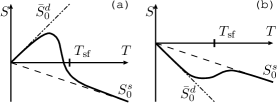
Figure 1: The effect of spin-fluctuation drag on the thermopower $S(T)$ is schematically shown. The bold lines are drawn to interpolate the two linear relations, $S(T)=\bar{S}_{0}^{d}$ and $\bar{S}_{0}^{s}$. The low temperature $\bar{S}_{0}^{d}$ in (79) is due to drag of those heavy electrons pertaining to the spin fluctuations, while the normal diffusion term $S\simeq{S}_{0}^{s}$ due to light conduction electrons appear at high temperature $T\gg\bar{T}\simeq T_{\rm sf}$, a spin-fluctuation temperature. The left (a) is for $\bar{S}_{0}^{d}>0$, while (b) for $\bar{S}_{0}^{d}<0$. The latter is compared with ${\rm RCo_{2}}$ (R=Sc, Y and Lu) by Gratz $et$ $al$.[12, 13, 14]

Takabatake $et$ $al$.[16] have shown experimentally by applying the magnetic field of 15T that an S-shaped structure in $S(T)$ of ${\rm CaFe_{4}Sb_{12}}$ observed at low $T<\bar{T}\simeq 50$K is suppressed to yield a normal $T$-linear diffusion term. This is consistent with our result for $\bar{S}_{0}^{d}<0$, $S_{0}^{s}>0$ and $|\bar{S}_{0}^{d}/S_{0}^{s}|\simeq 8$. In this case, the conduction band for $S_{0}^{s}$ consists mainly of 5$p$ states of antimony. Moreover, they have shown that the temperature dependence of the spin-fluctuation contribution $\Delta S=S-S_{0}^{s}$ is not monotonic. To explain this theoretically goes beyond the scope of this paper, as it requires us to solve the transport equations concretely. Similarly known before were the low temperature minima in the thermopower of ${\rm RCo_{2}}$ (R=Sc, Y and Lu), which had been stressed by Gratz $et$ $al$.[12, 13, 14] as the experimental evidence of paramagnon drag. Their results can be compared with our result for $\bar{S}_{0}^{d}\ll S_{0}^{s}<0$ in figure 1 (b).

On the correction terms, it is generally expected that the $d$ electron contribution $\Delta S_{d}$ will become more important than $\Delta S_{s}$ when the $d$ electron current becomes relevant indeed. As discussed in section 4.2, we have to consider two sources of contributions, one due to the equilibrium effect and the other due to the non-equilibrium effect in section 5. Interestingly, we find that both give the same temperature dependence, $S(T)=\alpha T+\beta T^{3}\log T^{-1}$ away from the QCP. Nevertheless, we notice an important difference. While we observe $\beta\propto 1/K_{0}^{4}$ from the results of the last section, $\beta$ expected from a correction term in (40) has an extra factor of $1/K_{0}^{2}$.[3] This means that the equilibrium effect becomes more important. We suspect that this would hold true at the QCP too, although there has been no definite calculation deriving the corresponding free energy correction $\propto T^{5/3}$ in accordance with our result.

In any case, we remark that the relative magnitude of the electron numbers $n_{s}$ and $n_{d}$ may have an effect on the correction terms, the sign of which will depend on the factor $en=e(n_{s}+n_{d})$, that is, the direction of the net current. In most cases where the model applies, the current carrier in the heavy-electron band will be hole like. Moreover, we generally expect that $|n_{s}|$ will not exceed $|n_{d}|$, or the net current would be hole-like, $e(n_{s}+n_{d})>0$. Accordingly, $\Delta S_{i}>0$ (cf. (41)). This is consistent with a model calculation of the spin fluctuation effect on the resistivity, where Jullien $et$ $al.$[21, 11] pointed out the important role of the parameter $\xi=k_{F,c}/k_{F,d}$ on the transport properties of spin fluctuations systems. We observe the dependence in our results of (76) and (77). To compare their numerical results with experiments, they should choose $\xi\leq 1$ generically, that is, $|n_{s}|\mathrel{\mathchoice{\lower 3.0pt\vbox{\halign{$\m@th \displaystyle\hfill#\hfil$\cr<\crcr\sim\crcr}}}{\lower 3.0pt\vbox{\halign{$\m@th \textstyle\hfill#\hfil$\cr<\crcr\sim\crcr}}}{\lower 3.0pt\vbox{\halign{$\m@th \scriptstyle\hfill#\hfil$\cr<\crcr\sim\crcr}}}{\lower 3.0pt\vbox{\halign{$\m@th \scriptscriptstyle\hfill#\hfil$\cr<\crcr\sim\crcr}}}}|n_{d}|$.

To conclude, let us fit the low-temperature experimental data for $S(T)$ of $\rm AFe_{4}Sb_{12}$ $\rm(A=Ba,Sr,Ca)$ reported by Matsuoka $et$ $al.$[15] with

$$S(T)=\alpha T+\beta T\left(\frac{T}{\bar{T}}\right)^{2}\log\frac{\delta+\left(T/\bar{T}\right)^{2}}{\left(T/\bar{T}\right)^{2}},$$ (80)

where $\alpha$, $\beta$, $\bar{T}$ and $\delta$ are regarded as parameters. In table 1, we present the fitting parameters obtained for $\delta=4$ by the least squares fits of the low temperature part of the data for $T\mathrel{\mathchoice{\lower 3.0pt\vbox{\halign{$\m@th \displaystyle\hfill#\hfil$\cr<\crcr\sim\crcr}}}{\lower 3.0pt\vbox{\halign{$\m@th \textstyle\hfill#\hfil$\cr<\crcr\sim\crcr}}}{\lower 3.0pt\vbox{\halign{$\m@th \scriptstyle\hfill#\hfil$\cr<\crcr\sim\crcr}}}{\lower 3.0pt\vbox{\halign{$\m@th \scriptscriptstyle\hfill#\hfil$\cr<\crcr\sim\crcr}}}}17$K $(<\bar{T})$. The results are shown in figure 2, along with the experimental data points. We find that $\alpha$’s do not depend much on the other parameters, and the ratios of $\beta$ and $\bar{T}$ between materials are nearly independent of $\delta$. The relatively large values for $\alpha$ and $\beta$ will be more properly ascribed to the heavier $d$ band than to the conduction band, in accordance with our result. Note that these coefficients are susceptible to the equilibrium effect of mass enhancement,[3, 4] which we did not take into account explicitly (cf. section 4.2). The positive $\beta$ implies that the net current is in the hole-like direction. The relative material dependence of $\beta$ in table 1 may be qualitatively compared with the observed static uniform susceptibility $\chi_{0}\propto\rho_{d}/K_{0}^{2}$, that is, $\chi_{0}({\rm BaFe_{4}Sb_{12}}):\chi_{0}({\rm SrFe_{4}Sb_{12}}):\chi_{0}({\rm CaFe_{4}Sb_{12}})\simeq 1:1.6:2.5$.

Figure 2: The points are the experimental data of $S(T)$ for $\rm AFe_{4}Sb_{12}$ $\rm(A=Ba,Sr,Ca)$.[15] The lines are the least squares fits by the theoretical expression in (80) with the parameters given in table 1.

Table 1: Parameters to fit the thermopower of $\rm AFe_{4}Sr_{12}$ in figure 2.

• 	$\alpha$ [$\rm\mu V/K^{2}$]	$\beta$ [$\rm\mu V/K^{2}$]	$\bar{T}$ [K]
  $\rm BaFe_{4}Sb_{12}$	$-0.35$	1.5	48
  $\rm SrFe_{4}Sb_{12}$	$-0.74$	1.6	37
  $\rm CaFe_{4}Sb_{12}$	$-1.4\hbox{\phantom{\footnotesize\rm 0}}$	3.7	58

Appendix A Formal transport theory

The formal expressions for resistivity and thermopower referred to in the main text are derived by adapting a general variational method of Ziman,[24] according to which $\Phi^{s}$ in (13) and $\Phi^{d}$ in (24) are regarded as variational trial functions. Below we substitute $\eta_{i}\Phi^{i}$ for $\Phi^{i}$ ($i=s,d$), and take variation with respect to the arbitrary parameters $\eta_{i}$.

On the one hand, the microscopic entropy production rate corresponding to (29) is given by

$$\dot{S}_{\rm scatt} = \frac{1}{T^{2}}\sum_{k,q}\left(\eta_{s}\Phi_{k}^{s}-\eta_{s}\Phi_{k+q}^{s}+\eta_{d}\Phi_{q}^{d}\right)^{2}{\cal P}^{k+q}_{kq}$$ (81)

$$\equiv\frac{1}{T}\sum_{i,j=s,d}P_{ij}\eta_{i}\eta_{j}.$$

The components of the matrix $P_{ij}$ defined in (81) are explicitly given by

$$P_{ss} = \frac{1}{T}\sum_{k,q}{\cal P}^{k+q}_{kq}\left(\Phi_{k}^{s}-\Phi_{k+q}^{s}\right)^{2},$$ (82)

$$P_{sd}=P_{ds} = \frac{1}{T}\sum_{k,q}{\cal P}^{k+q}_{kq}\left(\Phi_{k}^{s}-\Phi_{k+q}^{s}\right)\Phi_{q}^{d},$$ (83)

$$P_{dd} = \frac{1}{T}\sum_{k,q}{\cal P}^{k+q}_{kq}(\Phi_{q}^{d})^{2}.$$ (84)

In (81), not only emission of a paramagnon corresponding to (29), but the reverse absorption process is also taken into account. In the special case of the full drag without Umklapp processes, there holds the relation $\Phi_{k+q}^{s}-\Phi_{k}^{s}=\Phi_{q}^{d}$ by (30), so that we get the following identities,

$$P_{ss}=P_{dd}=-P_{sd}.$$ (85)

On the other hand, the macroscopic entropy production is given by

$$\dot{S}_{\rm macro}=\frac{{\bi J}\cdot{\bi E}}{T}+{\bi U}\cdot\nabla\frac{1}{T}.$$ (86)

In the linear response regime, the electric current ${\bi J}$ and the heat current ${\bi U}$ are written as

$${\bi J} = \eta_{s}{\bi J}[\Phi^{s}]+\eta_{d}{\bi J}[\Phi^{d}],$$ (87)

$${\bi U} = \eta_{s}{\bi U}[\Phi^{s}]+\eta_{d}{\bi U}[\Phi^{d}],$$ (88)

where ${\bi J}[\Phi^{i}]$ denotes the current flow caused by $\Phi^{i}$ ($i=s,d$), i.e., ${\bi J}[\Phi^{i}]$ formally represents the part of the total current which depends linearly on $\Phi^{i}$. ${\bi U}[\Phi^{i}]$ is similarly defined. In general, these currents have different functional forms. It is remarked that ${\bi J}[\Phi^{i}]$ is not to be identified with the current in the $i$ band. Owing to the interband interaction, the distribution shift $\Phi^{i}$ in the $i$ band can induce a current in the other band.

The variational parameters $\eta_{i}$ are determined so as to maximize $\dot{S}_{\rm scatt}$ after equating $\dot{S}_{\rm scatt}$ and $\dot{S}_{\rm macro}$.[24] Substituting the solutions into (87) and (88), we obtain

$${\bi J}=\sum_{i,j=s,d}{\bi J}[\Phi^{i}](P^{-1})_{ij}\left({{\bi J}[\Phi^{j}]\cdot{\bi E}}-\frac{1}{T}{\bi U}[\Phi^{j}]\cdot\nabla T\right),$$ (89)

and

$${\bi U}=\sum_{i,j=s,d}{\bi U}[\Phi^{i}](P^{-1})_{ij}\left({{\bi J}[\Phi^{j}]\cdot{\bi E}}-\frac{1}{T}{\bi U}[\Phi^{j}]\cdot\nabla T\right),$$ (90)

where $(P^{-1})_{ij}$ is the inverse matrix of $P_{ij}$. For definiteness, let the applied field ${\bi E}$ and $\nabla T$ be in the direction of a unit vector ${\bi u}$. In an isotropic system, or in cubic symmetry, the results are expressed with the magnitudes $J[\Phi^{i}]={\bi J}[\Phi^{i}]\cdot{\bi u}$ and $U[\Phi^{i}]={\bi U}[\Phi^{i}]\cdot{\bi u}$. From (89), we obtain the electrical conductivity,

$$\sigma=\sum_{l,m=s,d}{J}[\Phi^{l}](P^{-1})_{lm}{J}[\Phi^{m}].$$

The resistivity $R=\sigma^{-1}$ is given by

$$R=R_{0}(T)\frac{\displaystyle{1-\frac{P_{sd}P_{ds}}{P_{ss}P_{dd}}}}{\displaystyle 1+\left(\frac{{J}[\Phi^{d}]}{{J}[\Phi^{s}]}\right)^{2}\frac{P_{ss}}{P_{dd}}},$$ (91)

where

$$R_{0}(T)=\frac{P_{ss}}{({J}[\Phi^{s}])^{2}}.$$ (92)

The latter, given in (17), is the resistivity that we obtain when we have no spin-fluctuation drag. In fact, this is the central formula to explain an enhanced resistivity of a spin fluctuation system due to normal scattering processes with long-lived spin fluctuations.[19, 20, 5] According to (91), the $d$ electron drag modifies the resistivity in two ways. First, we note that the numerator in (91) vanishes in the full drag case, (85). This represents physically that a finite resistivity is brought about only with those scattering processes which can degrade the total net current. On the basis of a more realistic model, a proper treatment of Umklapp scattering processes could make the numerator a non-vanishing factor of order unity. Secondly, the positive factor in the denominator has the effect of suppressing the resistivity. This is due to an additional drag current of the $d$ electrons. When fully dragged, the $d$ electrons carry $n_{d}/n_{s}$ times as large current as the $s$ electrons, where $n_{d}/n_{s}$ is the ratio of the electron densities. In general, this would not be negligible quantitatively, and it might be so even qualitatively.

From the condition of no heat flow ${\bi U}=0$ for (90), we obtain the Seebeck coefficient,

$$S=\frac{1}{T}\frac{\displaystyle\sum_{l,m=s,d}{J}[\Phi^{l}](P^{-1})_{lm}{U}[\Phi^{m}]}{\displaystyle\sum_{l,m=s,d}{J}[\Phi^{l}](P^{-1})_{lm}{J}[\Phi^{m}]}.$$ (93)

From this we can obtain the result for the the full drag case of (85) formally as a special limit. It is expressed simply by the ratio of the total energy current to the total momentum current as

$$S=\frac{1}{T}\frac{{U}[\Phi^{s}]+{U}[\Phi^{d}]}{{J}[\Phi^{s}]+{J}[\Phi^{d}]}.$$ (94)

Indeed, the simple result in this limit is straightforwardly generalized to many-band models. It is owing to this simple property that we investigated this limit devotedly in the main text.

On the other side, the case without drag is obtained for ${U}[\Phi^{d}]={J}[\Phi^{d}]=0$ as

$$S_{0}^{s}=\frac{1}{T}\frac{{U}[\Phi^{s}]}{{J}[\Phi^{s}]},$$ (95)

as presented in (18). As a matter of fact, the no-drag results of (92) and (95) are directly derived without taking $\Phi^{d}$ into account from the beginning.

Appendix B Temperature dependence of ${\cal I}(T)$ at $\bar{\kappa}=0$

To evaluate ${\cal I}(T)$ in (59), we made the approximation as given in (61). We obtained (72) for ${\cal I}_{b}(T)$ in (64), which signifies the main correction term of $\Delta S\propto T^{5/3}$ in the quantum critical regime. The exponent 5/3 is the same as for the resistivity.[5] The derivation in section 5.3 indicates that the important contributions come from $\omega\simeq T$. In effect, this is the upper limit of the $\omega$ integral for $\bar{q}\mathrel{\mathchoice{\lower 3.0pt\vbox{\halign{$\m@th \displaystyle\hfill#\hfil$\cr>\crcr\sim\crcr}}}{\lower 3.0pt\vbox{\halign{$\m@th \textstyle\hfill#\hfil$\cr>\crcr\sim\crcr}}}{\lower 3.0pt\vbox{\halign{$\m@th \scriptstyle\hfill#\hfil$\cr>\crcr\sim\crcr}}}{\lower 3.0pt\vbox{\halign{$\m@th \scriptscriptstyle\hfill#\hfil$\cr>\crcr\sim\crcr}}}}\bar{q}_{0}$, and the high-energy cutoff is naturally provided by the Bose factor $n^{0}(\omega)$ in the integrand, without employing the approximation in (61). With this in mind, we can obtain the result for $\bar{\kappa}=0$ directly by transforming the integral and taking the limits for the bounds of integration as follows.

$${\cal I}_{b}(T)=\frac{1}{2\varepsilon_{F,d}^{2}}\int_{\bar{q}_{0}^{2}}^{2k_{F,s}/k_{F,d}}{{\rm d}\bar{q}^{2}}\int^{2\bar{q}}_{0}{\omega}{{\rm d}{\omega}}\frac{\partial}{\partial{\omega}}\left(\frac{{{\omega}}}{\bar{q}^{6}+\left(C{\omega}/\varepsilon_{F,d}\right)^{2}}\right)n^{0}(\omega)$$

$$\simeq\frac{1}{2\varepsilon_{F,d}^{2}}\int_{\bar{q}_{0}^{2}}^{2k_{F,s}/k_{F,d}}{{\rm d}\bar{q}^{2}}\int^{\infty}_{0}{\omega}{{\rm d}{\omega}}\frac{\partial}{\partial{\omega}}\left(\frac{{{\omega}}}{\bar{q}^{6}+\left(C{\omega}/\varepsilon_{F,d}\right)^{2}}\right)n^{0}(\omega)$$

$$=-\frac{T^{2/3}}{2\varepsilon_{F,d}^{2}}\int_{\bar{q}_{0}^{2}/T^{2/3}}^{2k_{F,s}/k_{F,d}/T^{2/3}}{{\rm d}v}\int^{\infty}_{0}\frac{{u}{{\rm d}u}}{v^{3}+\left(Cu/\varepsilon_{F,d}\right)^{2}}\frac{\partial}{\partial u}\left(\frac{u}{{\rm e}^{u}-1}\right)$$

$$\simeq-\frac{T^{2/3}}{2\varepsilon_{F,d}^{2}}\int_{0}^{\infty}{{\rm d}v}\int^{\infty}_{0}\frac{{u}{{\rm d}u}}{v^{3}+\left(Cu/\varepsilon_{F,d}\right)^{2}}\frac{\partial}{\partial u}\left(\frac{u}{{\rm e}^{u}-1}\right)$$

$$=-\frac{\pi}{3\sqrt{3}C^{4/3}}\left(\frac{T}{\varepsilon_{F,d}}\right)^{2/3}\int^{\infty}_{0}{{\rm d}u}u^{-1/3}\frac{\partial}{\partial u}\left(\frac{u}{{\rm e}^{u}-1}\right)$$

$$=1.10\frac{\pi}{3\sqrt{3}C^{4/3}}\left(\frac{T}{\varepsilon_{F,d}}\right)^{2/3}.$$ (96)

By comparing (96) and (72), we obtain ${c}^{-4/3}\simeq 1.10$, or

$${c}\simeq 0.928.$$ (97)

References

References

- [1] Saxena S S, Agarwal P, Ahhilan K, Grosche F M, Haselwimmer R K W, Steiner M J, Pugh E, Walker I R, Jullian S R, Monthoux P, Lonzarich G G, Huxley A, Sheikin I, Braithwaite D and Flouquet J 2000 Nature 406 587
- [2] Niklowitz P G, Beckers F, Lonzarich G G, Knebel G, Salce B, Thomasson J, Bernhoeft N, Braithwaite D and Flouquet J 2005 Phys. Rev. B 72 024424
- [3] Doniach S and Engelsberg S 1966 Phys. Rev. Lett. 17 750
- [4] Béal-Monod M T, Ma S K and Fredkin D R 1968 Phys. Rev. Lett. 20 929
- [5] Mathon J 1968 Proc. Roy. Soc. A 306 355
- [6] Moriya T 1985 Spin Fluctuations in Itinerant Electron Magnetism (Berin: Springer)
- [7] v Löhneysen H, Rosch A, Vojta M and Wölfle P 2007 Rev. Mod. Phys. 79 1015
- [8] Armbrüster H, Franz W, Schlabitz W and Steglich F 1979 J. Physique Colloq. 40 C4–150
- [9] Park J G and Očko M 1997 J. Phys.: Condens. Matter 9 4627
- [10] Iglesias-Sicardi J R, Jullien R and Coqblin B 1978 Phys. Rev. B 17 2366
- [11] Coqblin B, Iglesias-Sicardi J R and Jullien R 1978 Contemp. Phys. 19 327
- [12] Gratz E, Resel R, Burkov A T, Bauer E, Markosyan S S and Galatanu A 1995 J. Phys.: Condens. Matter 7 6687
- [13] Gratz E 1997 Physica B 237-238 470
- [14] Gratz E and Markosyan A S 2001 J. Phys.: Condens. Matter 13 R385
- [15] Matsuoka E, Hayashi K, Ikeda A, Tanaka K, Takabatake T and Matsumura M 2005 J. Phys. Soc. Jpn. 74 1382
- [16] Takabatake T, Matsuoka E, Narazu S, Hayashi K, Morimoto S, Sasakawa T, Umeo K and Sera M 2006 Physica B 383 93
- [17] Kaiser A B 1976 AIP Conf. Proc. 29 364
- [18] Behnia K, Jaccard D and Flouquet J 2004 J. Phys.: Condens. Matter 16 5187
- [19] Mills D L and Lederer P 1966 J. Phys. Chem. Solids 27 1805
- [20] Rice M J 1968 J. Appl. Phys. 39 958
- [21] Jullien R, B’eal-Monod M T and Coqblin B 1974 Phys. Rev. B 9 1441
- [22] Ueda K and Moriya T 1975 J. Phys. Soc. Jpn. 39 605
- [23] Izuyama T, Kim D J and Kubo R 1963 J. Phys. Soc. Jpn. 18 1025
- [24] Ziman J M 1960 Electrons and Phonons (Oxford: Clarendon Press)
- [25] Okabe T 1998 J. Phys. Soc. Jpn. 67 2792
- [26] Mott N F 1935 Proc. Roy. Soc. 47 571
- [27] Miyake K and Kohno H 2005 J. Phys. Soc. Jpn. 74 254