Thermodynamics of driven collisionless systems

Abstract

A statistical theory is presented which allows to calculate the stationary state achieved by a driven system after a process of collisionless relaxation. The theory is applied to study an electron beam driven by an external electric field. The Vlasov equation with appropriate boundary conditions is solved analytically and compared with the molecular dynamics simulation. A perfect agreement is found between the theory and the simulations. The full current-voltage phase diagram is constructed.

I Introduction

Unlike the equilibrium thermodynamics and statistical mechanics, which are well developed after the pioneering works of Boltzmann and Gibbs, our understanding of non-equilibrium thermodynamics is restricted to some special models and cases. Stochastic lattice gases have provided a fertile testing ground for studying non-equilibrium stationary states in driven systems MaDi99 ; derrida92 ; derrida93 . These models exhibit a variety of phase transition arising from a diffusive (collisional) relaxation. For some of these models local equilibrium and hydrodynamic equations have been derived rigorously BeSo07 .

There are, however, other physical systems for which the approach to final stationary state is through a process of collisionless relaxation Ly67 ; Pa90 ; ChSo98 ; Ch06 ; AnFa07 ; levin08 ; LePa08 . Gravitational systems and confined one component plasmas are just two such examples. For these systems the collision duration time diverges and the relaxation is governed by the collisionless Boltzmann (Vlasov) equation davidson01 . In the thermodynamic limit, the collisionless relaxation process leads to non-Maxwell-Boltzmann velocity distributions, even for stationary states without macroscopic currents. Unlike normal thermodynamic equilibrium, the stationary state which follows the collisionless relaxation depends explicitly on the initial distribution of particle positions and velocities. In spite of this complication, it was recently shown that it is possible to construct a statistical theory that quantitatively describes these states levin08 ; LePa08 .

Beams of electrons driven by accelerating vacuum devices, like the thermionic valves, diodes, and magnetrons, also do not relax to the Maxwell-Boltzmann distribution reiser94 . Unlike the driven stochastic lattice gases, these systems, however, are intrinsically collisionless. An important practical question concerns the kinetic temperature distribution in thermionic devices in which the directed velocity produced by the electric field is comparable to the thermal velocity chip06 . This is particularly the case for the transitional region between Child-Langmuir and no-cutoff regimes in magnetrons, where the electric potential becomes comparable to the thermal energy chip06 . Even when the final directed velocity is larger than the thermal velocity, there is a region near the emitting cathode where thermal effects are important. It is of great practical interest to determine the extent of these regions diode1 ; diode2 . Furthermore, since in these systems the collision duration time diverges, there is no local equilibrium, and one can not a priori postulate an equation of state relating the beam density and the beam temperature, as for adiabatic or isothermal processes. Instead, given the properties of thermionic filaments — such as say the velocity distribution of the emitted electrons — one should solve the boundary value problem posed by the Vlasov equation. The purpose of this Letter is to develop a theoretical framework which will allow us to study the relaxation dynamics and the stationary states of collisionless driven systems.

As a prototype of a collisionless driven system, we consider a beam of electrons, accelerated by an external electric field, traveling from an emitting (planar) cathode to a collecting (planar) anode across the device gap. The cathode, located at position $x=0$, is kept at electrostatic potential $\varphi(x=0)=0$ and is heated to temperature $T_{c}$, resulting in the emission of electrons. After traversing the device gap, these electrons are collected at the cold anode ($T_{a}\approx 0$) located at $x=L$ and kept at potential $\varphi(x=L)=V>0$. During the steady state operation, the region between the cathode and anode contains a total of $N$ electrons, resulting in a current density $j$. Our goal is to relate $j$, to the potential difference $V$, the number of electrons $N$, the device width $L$, and the cathode temperature $T_{c}$.

For planar electrodes, particle distribution transverse to the $x$ axis can be taken to be uniform. Furthermore, the one particle distribution function for a collisionless system in a steady state must satisfy the stationary Vlasov equation,

$$v{\partial f\over\partial x}+{e\over m}\nabla\varphi(x)\,{\partial f\over\partial v}=0,$$ (1)

where $e$ is the elementary charge, $m$ is the electron mass, and $f=f(x,v)$ is the static distribution function. In the thermodynamic limit, Vlasov equation becomes exact for particles interacting by long range potentials Br77 .

It can be readily seen that the distribution functions of the form $f(x,v)=f[\varepsilon(x,v)]$, where $\varepsilon$ is the mean particle energy, $\varepsilon\equiv mv^{2}/2-e\varphi(x)$, satisfy Eq. (1). Therefore, if $f(\varepsilon)$ is specified at $x=0$, $f$ is then also determined for any other position, provided that the electrostatic potential $\varphi(x)$ is known. This potential can, in turn, be calculated self-consistently from the solution of the Poisson equation

$$\frac{d^{2}\varphi(x)}{d\,x^{2}}={e\over\epsilon_{0}}\>n(x),$$ (2)

where the particle density $n(x)$ is given by $n(x)=\int_{v}f(\varepsilon)\,dv=\int_{v}f(mv^{2}/2-e\varphi(x))\,dv$, the total particle number is $N=A\int_{v}\int_{0}^{L}f\,dx\,dv$, and the transverse cross sectional area of the essentially 1D device is $A$. To represent both the thermal distribution near the cathode, and the fact that only particles with positive velocities actually move into the device gap, we choose at $x=0$ a unidirectional Maxwellian distribution of the form

$$f(x=0,v)=\>\cases{n_{0}\sqrt{2m\over\pi k_{B}T_{c}}\,\exp\left(-{m\,v^{2}\over 2k_{B}T_{c}}\right)\>\>{\rm if}\>\>v\geq 0,\cr 0\>\>{\rm if}\>\>v<0.}$$ (3)

where $k_{B}$ is the Boltzmann constant, $T_{c}$ is the cathode temperature, and $n_{0}$ is the beam density at the cathode after the stationary state is achieved. The value of $n_{0}$ can only be obtained once the full problem has been resolved. The distribution function over the length of the whole diode is then

$$f(x,v)=\>\cases{n_{0}\sqrt{2m\over\pi k_{B}T_{c}}\,\exp\left(-\frac{m\,v^{2}}{2k_{B}T_{c}}+\frac{e\varphi(x)}{k_{B}T_{c}}\right)\>{\rm if}\>v\geq v_{min}(x),\cr 0\>\>{\rm if}\>\>v<v_{min}(x).}$$ (4)

where $v_{min}(x)=\sqrt{2e\varphi(x)\over m}$.

Integrating the distribution function $f[\varepsilon(x,v)]$ over the possible values of velocity, we arrive at a nonlinear integro-differential equation for the electrostatic potential,

$$\frac{d^{2}\varphi}{d\,x^{2}}={Ne\over\varepsilon_{0}A}{e^{{e\varphi(x)\over k_{B}T_{c}}\,}{\rm Erfc}\left(\sqrt{e\varphi(x)\over k_{B}T_{c}}\right)\over\int e^{{e\varphi(x)\over k_{B}T_{c}}\,}{\rm Erfc}\left(\sqrt{e\varphi(x)\over k_{B}T_{c}}\right)dx}.$$ (5)

It is important to note the difference between this equation and the Poisson-Boltzmann equation obtained for usual collisional plasmas and electrolytes in the mean-field limit Le02 . Equation (5) can be solved numerically, to yield the electrostatic potential and the distribution function for the electron beam in the stationary state.

For systems with long range interactions, Vlasov equation should become exact in the thermodynamic limit. To confirm this for our system, we have performed molecular dynamics simulation of an equivalent one dimensional model. The simulated system consists of $N_{s}$ mutually interacting charged sheets of area $A$ — each containing $n_{s}$ electrons of the same velocity — moving along the $x$ axis, under the action of the external electric field produced by the grounded cathode $\varphi(0)=0$ and an anode kept at a fixed potential $\varphi(L)=V$. The interaction potential between the two sheets $G(x_{i},x_{j})$ is the Green’s function jack99 of the Laplace equation, $d^{2}G(x,y)/dx^{2}=1/L\>\delta(x-y)$ with the boundary conditions $G(x=0,y)=G(x=L,y)=0$. Solving this equation we obtain $G(x_{i},x_{j})=x_{{}_{<}}/L\>\big{(}x_{{}_{>}}/L-1\big{)}$, where $x_{<}$ and $x_{>}$ are the smaller and the larger of the two particle coordinates $x_{i}$ and $x_{j}$. The effective Hamiltonian for the sheet dynamics is then

$$H=\sum_{i}\left({m_{s}v_{i}^{2}\over 2}-{e_{s}V\over L}x_{i}\right)-{1\over 2}\>{e_{s}^{2}L\over\varepsilon_{0}A}\>\sum_{i,j}G(x_{i},x_{j}),$$ (6)

where $e_{s}=n_{s}e$ and $m_{s}=n_{s}m$ are the charge and mass of each sheet respectively. The acceleration of each simulated sheet then follows from the canonical equations of motion,

$$\dot{v}={eV\over mL}+{Ne^{2}\over 2\varepsilon_{0}mA}\left[\left({n^{[left]}-n^{[right]}\over N_{s}}\right)-\left(1-2\,{\overline{x}\over L}\right)\right],$$ (7)

where $n^{[left(right)]}$ is the number of sheets to the left(right) of the one considered, and $\overline{x}$ denotes the positional average $\overline{x}=\sum_{j}x_{j}/N_{s}$. Since $0\leq\overline{x}\leq L$, from Eq. (7) one sees that the electron acceleration at the device entrance where $n^{[left]}\rightarrow 0$ and $n^{[right]}\rightarrow N_{s}$ satisfies $eV/mL-Ne^{2}/2\varepsilon_{0}mA<\dot{v}(x=0)<eV/mL$, which reveals that in space-charge dominated devices where $eV/mL<Ne^{2}/2\varepsilon_{0}mA$, acceleration at beam entrance may be zero or even negative pak01 . When the acceleration vanishes, the associated current is denoted as the limiting one. Since we wish to describe a hot cathode and a cycling current inside the device, we adopt the following strategy. We advance the simulation in small time steps, always obeying Eq. (7). Whenever a particle crosses the anode and exits the system, it is re-injected at the cathode position. At this point all the particles in a small region $\delta_{s}$ around the cathode are re-thermalized, so as to ensure that the distribution there keeps its original form of a truncated Maxwellian. The width $\delta_{s}$ must be sufficiently small, $\delta_{s}\ll L$, but apart from this condition its precise value is arbitrary. The simulations were performed with $\delta_{s}/L=0.01$ and $N_{s}=50,000$. In all cases we start with a uniform distribution of sheets and compute the observables only after the system reaches its final stationary state.

To compare the predictions of the theory with the results of the simulations, we consider the density and the temperature distributions inside the diode. The kinetic temperature is defined as

$$k_{B}\,T(x)=\overline{v^{2}}(x)-\overline{v}^{2}(x).$$ (8)

where the over-bar denotes the velocity average at a given position $x$. The theoretical averages are calculated using the distribution function $f[\varepsilon(x,v)]$, while in the simulations, the averages are performed over the particle velocities within narrow bins along the $x$ axis. Note that because of the asymmetry of the velocity distribution at $x=0$, $T(0)\neq T_{c}$.

It is convenient to scale space and time with the diode length $L$ and the plasma frequency $\omega_{p}^{2}\equiv Ne^{2}/\epsilon_{0}mLA$, respectively. Dimensionless coordinate and velocity can then be defined as $x^{*}=x/L$ and $v^{*}=v/L\omega_{p}$. In addition, Eqs. (7) and (4) show that adimensional voltage and adimensional temperature can be defined as $V^{*}=eV/mL^{2}\omega_{p}^{2}$ and $T^{*}=k_{B}T/mL^{2}\omega_{p}^{2}$, respectively, and serve as the control parameters for the system.

In Fig. 1(a) the scaled temperature $T^{*}$ is plotted against the scaled coordinate $x^{*}$. We consider $T_{c}^{*}=0.05$ and also consider a device operating at its limiting current, $\dot{v}(x=0)=0$. A striking feature of this plot is that the temperature drops rapidly as one moves away from cathode towards anode. We next study the dependence of scaled density $n^{*}(x^{*})=n(x)A\,L/N$ along the length of the diode. The density is very high near the cathode, where the average velocity is small. It then drops rapidly towards the anode, where particles are accelerated up to high speeds, see Fig. 1(b). Agreement between the simulations and the theory for both the kinetic temperature and density is excellent.

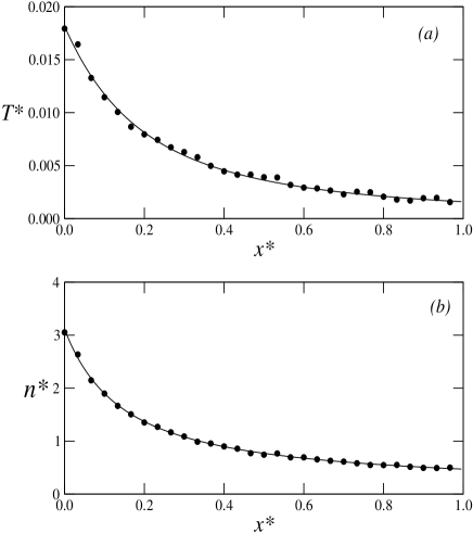
Figure 1: (a) Temperature and (b) density versus position in the case of the limiting current and $T_{c}^{*}=0.05$. Solid lines represent the theoretical results, while the circles are the results of the simulations.

We now study the current-voltage phase diagram of the device. In general, current is a function of the voltage drop, the temperature, the gap length, and the total charge of the device. However, by measuring the time in units of one over the plasma frequency $\omega_{p}^{-1}$, and the length in units of the gap length $L$, we can scale away two of these variables. The current density can be calculated using

$$j=-\,e\int v\,f\,dv.$$ (9)

Since in the steady state the current does not depend on either time or coordinate, integration along the $x$ axis and over the cross sectional area $A$ yields

$$jLA=-\,e\int v\,f\,dvdxd^{2}r_{\perp}.$$ (10)

Furthermore, since the current density is measured in units $[j]\sim[Nev/AL]$, rescaling it in terms of the gap length and the plasma frequency, we can write the reduced current density as $j^{*}=-ej/\varepsilon_{0}mL\omega_{p}^{3}$, which then satisfies

$$j^{*}=\overline{\overline{v^{*}}}\>\left(V^{*},T^{*}\right),$$ (11)

where $\overline{\overline{v^{*}}}$ is the reduced velocity averaged over all the particles. The reduced average velocity, in turn, must be a function of the two previously introduced control parameters: the reduced voltage and temperature. Eq.(11) is in fact a similarity transformation relating systems with different charge, length, temperature, and potential difference. In Fig. 2 we plot $j^{*}$ vs. $V^{*}$ for various $T^{*}$. The phase diagram provides all the information about the current-voltage characteristics for all possible planar diodes. The first feature to note is that all the different curves emanate from the limiting current backbone, which traces a temperature dependent path in the $j^{*}\times V^{*}$ plane. To the left of the limiting current border, indicated by the solid line in Fig. 2, the distribution function can no longer be described by a unidirectional Maxwellian, such as the expression (4). The transition resembles Bose-Einstein condensation (BEC). In the case of BEC — below the critical temperature — a macroscopically populated ground state appears, and only a fraction of particles remains in the excited states. Similarly, in the case of our diode, to the left of the limiting curve, part of the charge must be expelled from the system before a stationary state can be achieved. As $T_{c}^{*}\rightarrow\infty$, the voltage effects become negligible compared to the thermal ones, and the beam density becomes uniform across the gap. In this limit, it is possible to show that the dimensionless backbone curve asymptotes to a vertical line, $V^{*}=0.5$, Fig. 2.

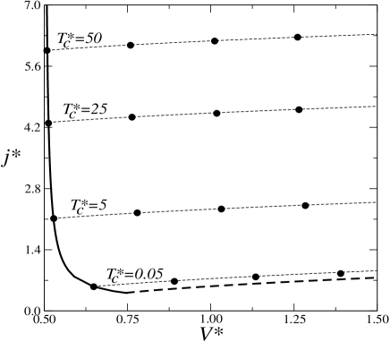
Figure 2: Characteristic curves of $j^{*}$ vs. $V^{*}$. The thick solid line represents the limiting current and the thick dashed line, the zero temperature limit. To the left of the solid curve, charge must be expelled from the system before a stationary state can be achieved. Dotted lines represent the theoretical results for the indicated temperatures. The circles are the results of the simulations at the same temperatures.

To conclude, we have studied the dynamics of collisionless driven systems. Unlike the stochastic lattice gasses which are significantly abstracted from reality, the models studied in this paper are very similar to real electronic devises, such as the thermionic valves, diodes, and magnetrons. Furthermore, differently from the lattice gases whose dynamics is diffusive, the distribution function of collisionless systems satisfies the Vlasov equation. For the class of driven systems introduced in this letter, the stationary state Vlasov equation can be solved exactly. The theory developed in this paper should, therefore, be relevant to the design and operation of real electronic devises.

It is important to stress that in the absence of collisions, a charged beam does not relax to an equilibrium with a known equation of state. In fact, the thermodynamic temperature is defined only in the vicinity of the hot emitting cathode. Away from the cathode, dynamics is controlled by the collisionless Vlasov equation, which has to be solved as a boundary value problem. Once the solution is obtained, all the macroscopic quantities can be determined via appropriate averages. The kinetic temperature is found to vary strongly across the device gap, precluding the use of conventional isothermal or adiabatic assumptions and of the hydrodynamic formalisms.

- (1) J. Marro and R. Dickman, Nonequilibrium phase transitions in lattice models, (Cambridge University Press, 1999).
- (2) B. Derrida, E. Domany, and D. Mukamel, J. Stat. Phys. 69, 667 (1992).
- (3) B. Derrida, S. A. Janowsky, J. L. Lebowitz, and E. R. Speer, J. Stat. Phys. 73, 813 (1993).
- (4) L. Bertini et al., J. Stat. Mech.: Theory and Experiment, P07014 (2007).
- (5) D. Lynden-Bell, Mon. Not. R. Astron. Soc. 136, 101 (1967).
- (6) T. Padmanabhan, Physics Reports 188, 285 (1990).
- (7) P.-H. Chavanis and J. Sommeria, Mon. Not. R. Astron. Soc. 296, 569 (1998).
- (8) P.-H. Chavanis, Physica A 359, 177 (2006).
- (9) A. Antoniazzi,1 D. Fanelli, J. Barré, P.-H. Chavanis, T. Dauxois, and S. Ruffo, Phys. Rev. E 75, 011112 (2007).
- (10) Y. Levin, R. Pakter, and T.N. Telles, Phys. Rev. Lett. 100, 040604, (2008).
- (11) Y. Levin, R. Pakter and F.B. Rizzato, Phys. Rev. E 78, 021130 (2008).
- (12) R.C. Davidson and H. Qin, Physics of Intense Charged Particle Beams in High Energy Accelerators (World Scientific, Singapore, 2001).
- (13) M. Reiser, Theory and Design of Charged Particle Beams, (Wiley-Interscience, 1994).
- (14) G.H. Goedecke, B.T. Davis, C. Chen, and C.V. Baker, Phys. Plasmas 12, 113104-1 (2005).
- (15) P. Martin and G. Donoso, Phys. Fluids B 1, 247 (1989).
- (16) N. Jelić, R. Schrittwieser, and S. Kuhn, Phys. Lett. A 246, 319 (1998).
- (17) W. Braun and K. Hepp, Comm. Math. Phys. 56, 101 (1977); A. Antoniazzi,1 F. Califano, D. Fanelli, and S. Ruffo, Phys. Rev. Lett. 98. 150602 (2007)
- (18) Y. Levin, Rep. Prog. Phys. 65, 1577 (2002).
- (19) J.D. Jackson, Classical Electrodynamics, (John Willey, New York, 1975).
- (20) F.B. Rizzato, R. Pakter, and Y. Levin, Phys. Plasmas 14, 110701 (2007); R. Pakter and F.B. Rizzato, Phys. Rev. Lett. 87, 04480 (2001).