Simulation study of shock reaction on porous material

Abstract

Direct modeling of porous materials under shock is a complex issue. We investigate such a system via the newly developed material-point method. The effects of shock strength and porosity size are the main concerns. For the same porosity, the effects of mean-void-size are checked. It is found that, local turbulence mixing and volume dissipation are two important mechanisms for transformation of kinetic energy to heat. When the porosity is very small, the shocked portion may arrive at a dynamical steady state; the voids in the downstream portion reflect back rarefactive waves and result in slight oscillations of mean density and pressure; for the same value of porosity, a larger mean-void-size makes a higher mean temperature. When the porosity becomes large, hydrodynamic quantities vary with time during the whole shock-loading procedure: after the initial stage, the mean density and pressure decrease, but the temperature increases with a higher rate. The distributions of local density, pressure, temperature and particle-velocity are generally non-Gaussian and vary with time. The changing rates depend on the porosity value, mean-void-size and shock strength. The stronger the loaded shock, the stronger the porosity effects. This work provides a supplement to experiments for the very quick procedures and reveals more fundamental mechanisms in energy and momentum transportation.

I Introduction

Porous materials have extensive applications in industrial and military fields as well as in our daily life. For example, people have long been using porous material to shield delicate objects, to protect things from impact. The porosity characteristics of the material may significantly influences its dynamical and thermodynamical behaviors. When a porous material is shocked, the cavities inside the sample may result in jets and influence its back velocityn1 . Cavity nucleation due to tension waves controls the spallation behavior of the materialn3 . Cavity collapse plays a prominent role in the initiation of energetic reactions in explosivesB2002 . Most studies on shocked porous materials in literature were experimentalP1 ; Porous1 ; Porous2 ; Porous4 ; Gray2003 ; Porous8 and theoretical investigationsPastine1970 ; Porous3 ; Porous5 ; Porous6 ; Porous8 ; WuJing1995 ; WuJing1996 ; GengWuTanCaiJing . Most of them were focused on the Hugoniots and equations of state. Due to the inhomogeneities of the material, the underlying thermodynamical processes in the shocked body are very complex and far from well-understanding. Understanding these processes plays a fundamental role in the field and may present helpful information in material preparation.

From the simulation side, molecular dynamics can discover some atomistic mechanisms of shock-induced void collapsePorous7 ; Yang , but the spatial and temporal scales it may cover are too small compared with experimentally measurable ones. When treating with the dynamics of structured and/or porous materials, traditional simulation methods, both the Eulerian and Lagrangian ones, encountered severe difficulties. The material under investigation is generally highly distorted during the collapsing of cavities. The Eulerian description is not convenient to tracking interfaces. When the Lagrangian formulation is used, the original element mesh becomes distorted so significantly that the mesh has to be re-zoned to restore proper shapes of elements. The state fields of mass density, velocities and stresses must be mapped from the distorted mesh to the newly generated one. This mapping procedure is not a straightforward task, and introduces errors. In this study, we will use a newly developed mixed method, material-point method, to investigate the shock properties of porous materials.

The material-point method was originally introduced in fluid dynamics by Harlow, et alH1964 and extended to solid mechanics by Burgess, et al MPM , then developed by various researchers, including usJPCM2007 ; CTP2008 ; JPD2008 . At each time step, calculations consist of two parts: a Lagrangian part and a convective one. Firstly, the computational mesh deforms with the body, and is used to determine the strain increment, and the stresses in the sequel. Then, the new position of the computational mesh is chosen (particularly, it may be the previous one), and the velocity field is mapped from the particles to the mesh nodes. Nodal velocities are determined using the equivalence of momentum calculated for the particles and for the computational grid. The method not only takes advantages of both the Lagrangian and Eulerian algorithms but makes it possible to avoid their drawbacks as well.

The following part of the paper is planned as follows. Section II presents the theoretical model of the material under consideration. Section III describes briefly the numerical scheme. Simulation results are shown and analyzed in section IV. Section V makes the conclusion.

II Theoretical model of the material

In this study the material is assumed to follow an associative von Mises plasticity model with linear kinematic and isotropic hardeningCModel . Introducing a linear isotropic elastic relation, the volumetric plastic strain is zero, leading to a deviatoric-volumetric decoupling. So, it is convenient to split the stress and strain tensors, $\bm{\sigma}$ and $\bm{\varepsilon}$, as

$$\bm{\sigma} = \mathbf{s}-P\mathbf{I},P=-\frac{1}{3}\verb|Tr|(\bm{\sigma})\mathtt{,}$$ (1)

$$\bm{\varepsilon} = \mathbf{e}+\frac{1}{3}\theta\mathbf{I},\theta=\frac{1}{3}\verb|Tr|(\bm{\varepsilon})\mathtt{,}$$ (2)

where $P$ is the pressure scalar, $\mathbf{s}$ the deviatoric stress tensor, and $\mathbf{e}$ the deviatoric strain. The strain $\mathbf{e}$ is generally decomposed as $\mathbf{e}=\mathbf{e}^{e}+\mathbf{e}^{p}$, where $\mathbf{e}^{e}$ and $\mathbf{e}^{p}$ are the traceless elastic and plastic components, respectively. The material shows a linear elastic response until the von Mises yield criterion,

$$\sqrt{\frac{3}{2}}\left\|\mathbf{s}\right\|=\sigma_{Y}\mathtt{,}$$ (3)

is reached, where $\sigma_{Y}$ is the plastic yield stress. The yield $\sigma_{Y}$ increases linearly with the second invariant of the plastic strain tensor $\mathbf{e}^{p}$, i.e.,

$$\sigma_{Y}=\sigma_{Y0}+E_{\tan}\left\|\mathbf{e}^{p}\right\|\mathtt{,}$$ (4)

where $\sigma_{Y0}$ is the initial yield stress and $E_{\tan}$ the tangential module. The deviatoric stress $\mathbf{s}$ is calculated by

$$\mathbf{s}=\frac{E}{1+\nu}\mathbf{e}^{e}\mathtt{,}$$ (5)

where $E$ is the Yang’s module and $\nu$ the Poisson’s ratio. Denote the initial material density and sound speed by $\rho_{0}$ and $c_{0}$, respectively. The shock speed $U_{s}$ and the particle speed $U_{p}$ after the shock follows a linear relation, $U_{s}=c_{0}+\lambda U_{p}$, where $\lambda$ is a characteristic coefficient of material. The pressure $P$ is calculated by using the Mie-Grüneissen state of equation which can be written as

$$P-P_{H}=\frac{\gamma(V)}{V}[E-E_{H}(V_{H})]$$ (6)

This description consults the Rankine-Hugoniot curve. In Eq.(6), $P_{H}$, $V_{H}$ and $E_{H}$ are pressure, specific volume and energy on the Rankine-Hugoniot curve, respectively. The relation between $P_{H}$ and $V_{H}$ can be estimated by experiment and can be written as

$$P_{H}=\left\{\begin{array}[]{ll}\frac{\rho_{0}c_{0}^{2}(1-\frac{V_{H}}{V_{0}})}{(\lambda-1)^{2}(\frac{\lambda}{\lambda-1}\times\frac{V_{H}}{V_{0}}-1)^{2}},&V_{H}\leq V_{0}\\ \rho_{0}c_{0}^{2}(\frac{V_{H}}{V_{0}}-1),&V_{H}>V_{0}\end{array}\right.$$ (7)

In this paper, the transformation of specific internal energy $E-E_{H}(V_{H})$ is taken as the plastic energy. Both the shock compression and the plastic work cause the increasing of temperature. The increasing of temperature from shock compression can be calculated as:

$$\frac{\mathrm{d}T_{H}}{\mathrm{d}V_{H}}=\frac{c_{0}^{2}\cdot\lambda(V_{0}-V_{H})^{2}}{c_{v}\big{[}(\lambda-1)V_{0}-\lambda V_{H}\big{]}^{3}}-\frac{\gamma(V)}{V_{H}}T_{H}.$$ (8)

where $c_{v}$ is the specific heat. Eq.(8) can be resulted with thermal equation and the Mie-Grüneissen state of equationexplosion . The increasing of temperature from plastic work can be calculated as:

$$\mathrm{d}T_{p}=\frac{\mathrm{d}W_{p}}{c_{v}}$$ (9)

Both the Eq.(8) and the Eq.(9) can be written as the form of increment.

In this paper the sample material is aluminum. The corresponding parameters are $\rho_{0}=2700$ kg/m³, $E=69$ Mpa, $\nu=0.33$, $\sigma_{Y0}=120$ Mpa, $E_{\tan}=384$ MPa, $c_{0}=5.35$ km/s, $\lambda=1.34$, $c_{v}=880$ J/(Kg$\cdot$K), $k=237$ W/(m$\cdot$K) and $\gamma_{0}=1.96$ when the pressure is below $270$ GPa. The initial temperature of the material is 300 K.

III Outline of the numerical scheme

As a particle method, the material point method discretizes the continuum bodies with $N_{p}$ material particles. Each material particle carries the information of position $\mathbf{x}_{p}$, velocity $\mathbf{v}_{p}$, mass $m_{p}$, density $\rho_{p}$, stress tensor $\bm{\sigma}_{p}$ , strain tensor $\bm{\varepsilon}_{p}$ and all other internal state variables necessary for the constitutive model, where $p$ is the index of particle. At each time step, the mass and velocities of the material particles are mapped onto the background computational mesh. The mapped momentum at node $i$ is obtained by $m_{i}\mathbf{v}_{i}=\sum_{p}m_{p}\mathbf{v}_{p}N_{i}(\mathbf{x}_{p})$, where $N_{i}$ is the element shape function and the nodal mass $m_{i}$ reads $m_{i}=\sum_{p}m_{p}N_{i}(\mathbf{x}_{p}).$ Suppose that a computational mesh is constructed of eight-node cells for three-dimensional problems, then the shape function is defined as

$$N_{i}=\frac{1}{8}(1+\xi\xi_{i})(1+\eta\eta_{i})(1+\varsigma\varsigma_{i})\mathtt{,}$$ (10)

where $\xi$,$\eta$,$\varsigma$ are the natural coordinates of the material particle in the cell along the x-, y-, and z-directions, respectively, $\xi_{i}$,$\eta_{i}$,$\varsigma_{i}$ take corresponding nodal values $\pm 1$. The mass of each particle is equal and fixed, so the mass conservation equation, $\mathrm{d}\rho/\mathrm{d}t+\rho\nabla\cdot\mathbf{v}=0$, is automatically satisfied. The momentum equation reads,

$$\rho\mathrm{d}\mathbf{v/}\mathrm{d}t=\nabla\cdot\bm{\sigma}+\rho\mathbf{b}\mathtt{,}$$ (11)

where $\rho$ is the mass density, $\mathbf{v}$ the velocity, $\bm{\sigma}$ the stress tensor and $\mathbf{b}$ the body force. Equation (11) is solved on a finite element mesh in a lagrangian frame. Its weak form is

$$\begin{array}[]{ll}&\int_{\Omega}{\rho\delta\mathbf{v}\cdot\mathrm{d}\mathbf{v/}\mathrm{d}t\mathrm{d}\Omega}+\int_{\Omega}{\delta(\mathbf{v}\nabla)\cdot\bm{\sigma}\mathrm{d}\Omega}-\int_{\Gamma_{t}}{\ \delta\mathbf{v}\cdot\mathbf{t}\mathrm{d}\Gamma}\\ &-\int_{\Omega}{\ \rho\delta\mathbf{v}\cdot\mathbf{b}\mathrm{d}\Omega}=0\mathtt{.}\end{array}$$ (12)

Since the continuum bodies is described with the use of a finite set of material particles, the mass density can be written as $\rho(\mathbf{x})=\sum_{p=1}^{N_{p}}{\ m_{p}\delta(\mathbf{x}-\mathbf{x}_{p})}$, where $\delta$ is the Dirac delta function with dimension of the inverse of volume. The substitution of $\rho(\mathbf{x})$ into the weak form of the momentum equation converts the integral to the sums of quantities evaluated at the material particles, namely,

$$m_{i}\mathrm{d}\mathbf{v}_{i}/\mathrm{d}t=(\mathbf{f}_{i})^{\mathrm{int}}+(\mathbf{f}_{i})^{\mathrm{ext}}\mathtt{,}$$ (13)

where the internal force vector is given by $\mathbf{f}_{i}{}^{\mathrm{int}}=-\sum_{p}^{N_{p}}{m_{p}\bm{\sigma}}_{p}{\cdot(\nabla N_{i})/\rho_{p}}$, and the external force vector reads $\mathbf{f}_{i}{}^{\mathrm{ext}}=\sum_{p=1}^{N_{p}}{N_{i}\mathbf{b}_{p}+\mathbf{f}_{i}^{c}}$, where the vector $\mathbf{f}_{i}^{c}$ is the contacting force between two bodies. In present paper, all colliding bodies are composed of the same material, and $\mathbf{f}_{i}^{c}$ is treated with in the same way as the internal force.

The nodal accelerations are calculated by Eq. (13) with an explicit time integrator. The critical time step satisfying the stability conditions is the ratio of the smallest cell size to the wave speed. Once the motion equations are solved on the cell nodes, the new nodal values of acceleration are used to update the velocity of the material particles. The strain increment for each material particle is determined using the gradient of nodal basis function evaluated at the position of the material particle. The corresponding stress increment can be found from the constitutive model. The internal state variables can also be completely updated. The computational mesh may be the original one or a newly defined one, choose for convenience, for the next time step. More details of the algorithm is referred to JPD2008 ; CTP2008 .

Figure 1: (in JPG format) Snapshots of the shocked porous metal. $\delta=1.03$, t=250 ns. (a) Contour of pressure, (b) contour of temperature. The unit of length in this figure is 10 $\mu$m. From blue to red, the contour value increases. The unit of contour is Mpa in (a) and is K in (b). The initial velocities of the flyer and target are $\pm v_{init}=\pm 1000$ m/s in this case.

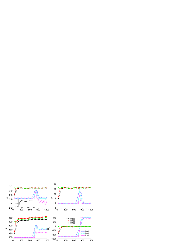
Figure 2: (Color online) Variations of mean density, pressure, temperature and particle velocity with time. The height of the measured domain are h= 800 $\mu$m, 400$\mu$m and 100 $\mu$m, respectively, as shown in the legends. “B" and “T" in the legends means the measured domains are at the bottom and top of the target body, respectively. The units of density, pressure, temperature, particle velocity and time are g/cm³, Gpa, K, m/s and ns, respectively.

Figure 3: (in JPG format) Configuration with temperature contour at time t=1.15 $\mu$s. Other parameters are referred to Fig.1 and Fig.2. The unit of temperature is K.

IV Results of numerical experiments

In the present study the porous material is fabricated by a solid material body with an amount of voids randomly embedded. The porosity $\delta$ is defined as $\delta=\rho_{0}/\rho$, where $\rho_{0}$ is the original density of the solid body and $\rho$ is the mean density of porous material. The porosity $\delta$ in the simulated system is controlled by the total number $N_{void}$ and mean size $r_{void}$ of voids embedded. The shock wave to the target porous metal is loaded via colliding by a second body. For the convenience of analysis, we set the configurations and velocities of the two colliding porous bodies symmetric about their impact interface. The initial velocities of the two colliding bodies are along the vertical direction and denoted as $\pm v_{init}$. The impact interface is set at $y=0$. Periodic boundary conditions are used in the horizontal directions, which means the investigated real system is composed of many of the simulated ones aligned periodically in the horizontal direction. We regarded the upper porous body as the target, the lower one as the flyer. Compared with experiments where the target is initially static, the initial velocity of the flyer is $2v_{init}$. In this study we focus on the two-dimensional case. The computational unit is 2 mm in width, as shown in Fig.1. When we are mainly interested in the loading procedure of shock wave to porous body, we require that each simulated body has an enough height so that the rarefactive waves from the upper and lower free surfaces do not affect the physical procedure within the time scale under investigation.

Figure 1 shows two snapshots of such a process, where Fig.1(a) shows the contour of pressure and Fig.1(b) shows the contour of temperature. The snapshots show clearly that, different from the case with perfect solid material, there is no stable shock wave in the porous materials. When the compressive waves arrive at a cavity, rarefactive waves are reflected back and propagate within the compressed portion, which destroys the original possible equilibrium state there. Even thus, for the convenience of description, we still refer the compressive waves to shock waves. Correspondingly, the values of physical quantities, such as the particle velocity, density, pressure, temperature, etc, are corresponding mean values calculated in a region $\Omega$ with $y_{1}\leq y\leq y_{2}$. We will investigate the effects of initial shock strength and porosity value.

IV.1 Cases with porosity $\delta$=1.03

We first study the case with $r_{void}$ =50 $\mu$m and the velocity $v_{init}$ = 1000 m/s, which means the flyer velocity relative to the target is 2000 m/s. The flyer begins to contact the target at the time t = 0. Figure 2 shows the variations of mean density, pressure, temperature and particle velocity with time. These values are dynamically measured in a bottom and a top domains, respectively. The height of the target body is 5 mm in this case. The height of the measured domains are h=800 $\mu$m, 400 $\mu$m and 100 $\mu$m, respectively. For the bottom domain, we choose $y_{1}=100\mu$m. For the top domain, $y_{2}$ takes the y-coordinate of the highest material-particle. The lines with solid symbols are measured values from the bottom and the lines with empty symbols are measured values from the top. From the figure, we get the following information: When the shock waves propagate within the bottom domain $\Omega_{b}$, the measured mean density, pressure and temperature increase nearly linearly with time, up to about t= 150 ns for the case of h=800 $\mu$m, then further to increase with a decreasing changing rate. The three quantities arrive at their first maximum values, 3.14g/cm³, 16.7GPa, and 432K, at the time t=250 ns. At this time the shock front has passed the downstream boundary, $y=810\mu$m, of the measured domain. (See Fig. 1.) The time delay is due to dispersion of shock wave in porous media. The followed concave in either of the $\rho$-,P-,T-curves at about t = 450 ns shows a downloading phenomenon. The phenomenon is resulted from rarefactive waves reflected back from the cavities downstream neighboring to the measured domain. The values of $\rho$ and P increase and recover to their steady values after that, but the temperature get a higher value. The secondary loading-phenomenon is due to the colliding of the upstream and downstream walls during the collapsing of cavities. Within the following period the density and pressure keep nearly constants, while the temperature still increases very slowly. The weak fluctuations in the $\rho$, P, T curves after $t=650$ ns result from the putting-in of compressive and rarefactive waves from the two boundaries of the measured domain $\Omega_{b}$. The visco-plastic work by these wave series makes the temperature increase slowly. Since the configurations and velocities of the flyer and target are symmetric about the plane $y=0$, the vertical component of particle velocity, $u_{y}$, is about 0 m/s, the horizontal component $u_{x}$ first increases with time, then oscillates around a small value which is nearly zero. The lines with empty symbols show that the shock waves arrive at the top free surface at about t= 800 ns, then rarefactive waves are reflected back into the target body. Within the time scale shown in the figure, for the cases with h=800 $\mu$m and 400 $\mu$m, the density (or pressure) recovers to a value being slightly larger than its initial one, but the remained temperature is about 60K higher than the initial temperature and is still increasing; for the case with h=100 $\mu$m, evident oscillations are found in the curve of density after t=900 ns. To understand this, we show in Fig.3 the top portion of the configuration with temperature contour for the time t=1.15 $\mu$s, from which we can find jetting phenomena at the upper free surface. During the downloading procedure, the top of the porous body moves upwards with a velocity being about 877 m/s. From the same data used in Fig.1, we can get the mutual dependence of the hydrodynamical quantities. The initial transient stage and the final oscillatory steady state are clearly observable. Due to existence of the randomly distributed voids, waves with various wave vectors and frequencies propagate within the shocked sample material. When the measured domain becomes smaller, more detailed wave structures may be found. Figure 2 shows clearly this trend.

It is interesting to check more carefully the procedure of approaching steady state. Figure 4 shows the standard deviations of the above four quantities versus time measured in the bottom domains. It is found that they increase quickly with time at the very beginning stage, then decrease nearly exponentially to their steady values. The standard deviation of $u_{y}$ is larger than that of $u_{x}$. The finite sizes of these steady values confirm our analysis above: what the system arrives is a steady state with local dynamical oscillations. When the height of the measured domain increases, the standard deviations of measured quantities become larger, at least in the transient period.

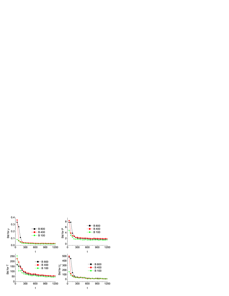
Figure 4: (Color online) Standard deviations(Std) of the local quantities averaged in various spatial scales. The heights of the measured domains are shown in the legends where “B" means the measured domains are at the bottom of the target body. The length and time units are $\mu$m and ns, respectively.

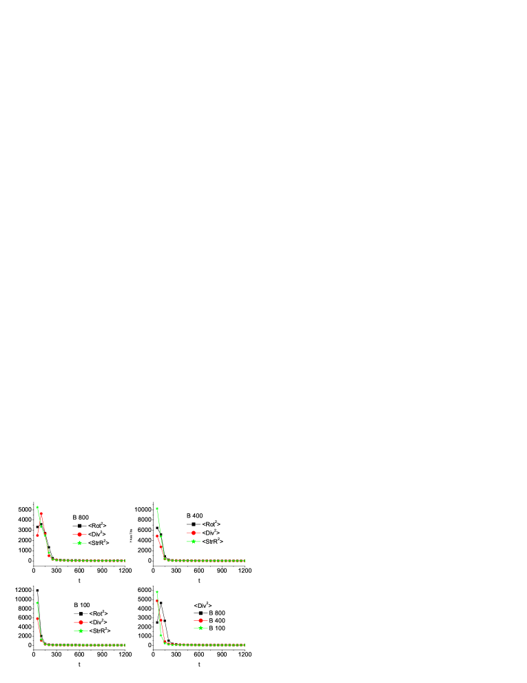
Figure 5: (Color online) Variations of the mean values squared of local rotation, divergence and strain rate with time. <…> in the legends denote the mean value of the corresponding quantity and “B" means the measured domains are at the bottom of the target body. The length and time units are $\mu$m and ns, respectively.

Figure 6: (in JPG format) Configurations with density contour (a), pressure contour (b), temperature contour (c) and velocity field (d) at time t=750 ns. The size of particle velocity is denoted by the length of arrow timed by 50. The units are the same as in Fig.2.

For the case with perfect crystal material, the increase of entropy result from only from the non-equilibrium procedure of the front of the shock waves. When cavities exist, the high plastic distortion of the materials surrounding the collapsed cavities contribute extra entropy increment. So the local rotation, Rot= $|\nabla\times\mathbf{u}|$, and divergence, Div= $|\nabla\cdot\mathbf{u}|$, make significance sense in describing shocked porous media. The local rotation $|\nabla\times\mathbf{u}|$ describes the circular flow and/or turbulence. The divergence $|\nabla\cdot\mathbf{u}|$ describes the changing rate of volume. They show important mechanisms of entropy and temperature increase in porous material. The former reflects the turbulence dissipation and the latter reflects the shock compression. Figure 5 shows the variations of their mean values squared with time. The behavior of strain rate $\bm{\dot{\varepsilon}}$ is plotted as a comparison. It is found that all the three quantities decrease nearly exponentially to their steady state values when shock waves pass the measured domain $\Omega$. The amplitude of steady strain rate is very close to that of the rotation. The amplitude of the divergence is a little larger for this case. Cavity collapse and new cavitation by the rarefactive waves are the main contributors to the local divergence. To understand better the fluctuations of the local density, pressure, temperature, particle velocity and the finite values of the rotation, divergence, we show in Fig.6 a portion of the configuration with density contour, pressure contour, temperature contour and velocity field at time $t=750$ns. In this case, there is a void around the position (510$\mu$m, 280$\mu$m).

We now checking the effects of the void size. Results for different void sizes are compared. There is no evident difference in the steady values of mean density, pressure and particle velocity. But larger voids contribute to a higher mean temperature. (See Fig.7.) As for effects on the mean value squared of the local rotation and divergence, the void size affect only the transient period, but not the steady values. See Fig.8, where the two cases correspond to different mean-void-sizes but the same value of porosity, $\delta=1.03$.

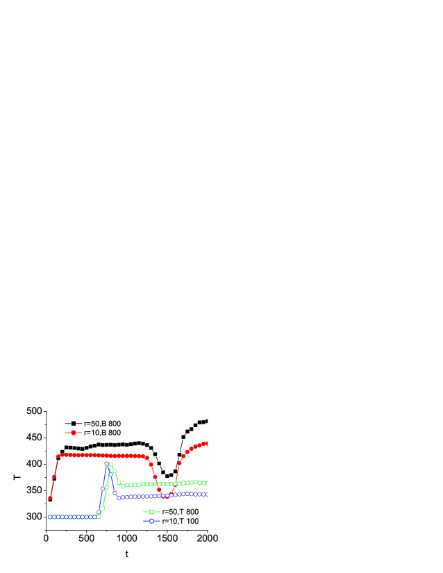
Figure 7: (Color online) Effects of the mean void size on the mean temperature. The mean void size $r$, position and height of the measured domain are shown in the legend. “B" and “T" means the measured domains are at the bottom and top of the target body, respectively. The length and time units are $\mu$m and ns, respectively.

Figure 8: (Color online) Effects of mean void size on the mean values squared of local rotation, divergence. The mean sizes of void are shown in the legends. The length and time units are $\mu$m and ns, respectively.

IV.2 Cases with porosity $\delta=1.4$

In this section we study the case with a higher porosity, $\delta$=1.4. For this case, the mean void size is r=10 $\mu$m. Figure 9 shows the variations of mean density, pressure, temperature and particle velocity with time. The initial velocity of the flyer and the target are $\pm v_{init}=1000$m/s. The physical quantities are averaged in a bottom and a top domains. Only the case with h=800 $\mu$m is shown. An evident difference from the low-porosity case with $\delta=1.03$ is that the mean density and pressure decrease with time after the initial stage. Correspondingly, the mean temperature increase with a higher rate. This is due to the rarefactive waves reflected back from the downstream voids. The reflected rarefactive waves make the shocked material a little looser and result in a relatively higher local divergence. The latter transforms more kinetic energy into heat. At the same time, a higher porosity means more voids embedded in the material, more jetting phenomena occur when being shocked. The jetting phenomena and the hitting of jetted material to the downstream walls of the voids make a significant increase of local temperature, local divergence and local rotation. The mean values squared of the local rotation, divergence and strain rate are shown in Fig.10. These quantities are measured in the bottom domain with h=800 $\mu$m. During the initial transient period, the turbulence dissipation makes the most significant contribution to temperature-increase in this case. In the later steady state, the three kinds of dissipation makes nearly the same contribution.

To understand better the inhomogeneity effects in the shocked portion of the porous body, we show the distributions of density, pressure, temperature and particle velocity at times t=1200ns, 1250ns and 1300ns in Fig.11. It is clear that these distributions generally deviate from the Gaussian distribution and vary with time. In Fig.12 we study the effects of initial impact velocity on the mean values of the density, pressure and temperature. It is clear that the decreasing rate of the mean density and the increasing rate of mean temperature increase when the initial shock wave becomes stronger. This means that the porosity effects become more significant when the loaded shock wave becomes stronger.

We now study porosity effects for a fixed shock strength. Figure 13 shows the mean density, and temperature versus time for various porosities. The initial velocity of the flyer and target are $\pm v_{init}$ = 1000m/s. When the porosity is very small, the decreasing rate with time of the mean density becomes higher as the porosity increases. But when the porosity becomes large, the mean density show more complex behavior.

Figure 9: (Color online) Variations of mean density, pressure, temperature and particle velocity with time. Here the porosity $\delta=1.4$ and initial flyer velocity relative to the target is $2v_{init}=2000$ m/s. The meanings of “B", “T" and units are the same as in Fig.2.

Figure 10: (Color online) Variations of the mean values squared of local rotation, divergence and strain rate with time. The unit of time is ns.

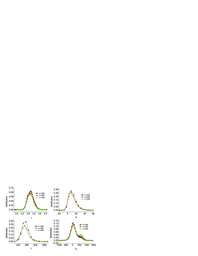
Figure 11: (Color online) Distribution of local density, pressure, temperature, particle velocity at various times. The units are the same as in Fig.2.

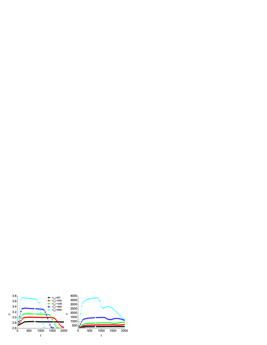
Figure 12: (Color online) Mean density and temperature versus time for various shock strengths. The initial velocity $v_{init}$ are shown in the legend. The units are the same as in Fig.2.

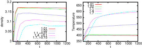
Figure 13: (Color online) Mean density and temperature versus time for various porosities. The values of porosity, 1.01,1.02,1.1,1.4,1.7 are shown in the legends. In the left figure, the lines for cases with $\delta=$1.1,1.4 and 1.7 are moved upwards by 0.01,0.1, and 0.15, respectively. The units are the same as in Fig.2.

V Conclusion

Thermodynamic properties of porous material under shock-reaction is studied via a direct simulation. The effects of shock strength, porosity value and the mean-void-size are checked carefully. It is found that, when the porosity is very small, the shocked portion will arrive at a dynamic steady state; the voids in the downstream portion reflect back rarefactive waves and result in slight oscillations of mean density and pressure; for the same value of porosity, a larger mean-void-size makes a higher mean temperature. When the porosity becomes larger, after the initial stage, the mean density and pressure decrease significantly with time. The distributions of local density, pressure, temperature and particle-velocity are generally non-Gaussian and vary with time. Different from the case with perfect solid material, local turbulence mixing and volume dissipation exist in the whole loading procedure and make the system temperature continuously increase. The changing rates depend on the porosity value, mean-void-size and shock strength. The stronger the loaded shock, the stronger the porosity effects. This work is supplementary to experimental investigations for the very quick procedures and reveals more fundamental mechanisms in energy and momentum transportation.

- (1) D.B.Reisman, W.G.Wolfer, A. Elsholz, and M.D. Furnish, J. Appl. Phys. 93, 8952 (2003).
- (2) E. Dekel, S. Eliezer, Z. Henis, E. Moshe, A. Ludmirsky, and I. B. Goldberg, J. Appl. Phys. 84, 4851 (1998); R. W. Minich, J. U. Cazamias, M. Kumar, and A. J. Schwartz, Metall. Mater. Trans. A 35, 2663 (2004).
- (3) N. K. Bourne, Shock Waves 11, 447 (2002).
- (4) R. K. Linde and D. N. Schmidt, J. Appl. Phys. 37, 3259 (1966).
- (5) R. R. Boade, J. Appl. Phys. 40, 3781 (1969).
- (6) B. M. Butcher, J. Appl. Phys. 45, 3864 (1974).
- (7) S. Bonnan and P. L. Hereil, J. Appl. Phys. 83, 5741 (1998).
- (8) G. T. Gray III, N. K. Bourne and J. C. F. Milett, J. Appl. Phys. 94, 6430 (2003).
- (9) A. D. Resnyansky, N. K. Bourne, J. Appl. Phys. 95, 1760 (2004).
- (10) D. J. Pastine, M. Lombardi, A. Chatterjee and W. Tchen, J. Appl. Phys. 41, 3144 (1970).
- (11) Z. P. Wang, J. Appl. Phys. 81, 7213 (1997).
- (12) J. Massoni, R. Saurel, G. Baudin and G. Demol, Phys. Fluid 11, 710 (1999).
- (13) L. Boshoff-Mostert and H. J. Viljoen, J. Appl. Phys. 86, 1245 (1999).
- (14) Q. Wu and F. Jing, Appl. Phys. Lett. 67, 49 (1995).
- (15) Q. Wu and F. Jing, J. Appl. Phys. 80, 4343 (1996).
- (16) H. Geng, Q. Wu, H. Tan, L. Cai and F. Jing, J. Appl. Phys. 92, 5924 (2002).
- (17) P. Erhart, E. M. Bringa, M. Kumar, and K. Albe, Phys. Rev. B 72, 052104 (2005).
- (18) Q. Yang, Guangcai Zhang, Aiguo Xu, Y. Zhao, Y. Li, Acta Phys. Sini. 57, 940 (2008) (in Chinese).
- (19) F. H. Harlow, 1964 Methods for Computational Physics, Vol. 3, 319-343, Adler B, Fernbach S, Rotenberg M (eds). Academic Press: New York .
- (20) D. Burgess, D. Sulsky, J. U. Brackbill, J. Comput. Phys. 103, 1 (1992).
- (21) Aiguo Xu, X F Pan, Guangcai Zhang and Jianshi Zhu, J. Phys.: Condens. Matter 19, 326212(2007).
- (22) X. F. Pan, Aiguo Xu, Guangcai Zhang, et al, Commun. Theor. Phys. 49, 1129 (2008).
- (23) X. F. Pan, AiguoXu ,Guangcai Zhang and Jianshi Zhu, J. Phys. D: Appl. Phys. 41, 015401 (2008).
- (24) F. Auricchio, L. B. da Veiga, Int. J. Numer. Meth. Engng 56 1375 (2003).
- (25) B. Zhang, et al. Explosion physics, Ordance Industry Press of China, 1997 Beijing.