Eddy viscosity and turbulent Schmidt number by kink-type instability of strong toroidal magnetic fields

Abstract

The potential of the nonaxisymmetric magnetic instability to transport angular momentum and to mix chemicals is probed considering the stability of a nearly uniform toroidal field between conducting cylinders with different rotation rates. The fluid between the cylinders is assumed as incompressible and to be of uniform density. With a linear theory the neutral-stability maps for $m=1$ are computed. Rigid rotation must be subAlfvénic to allow instability while for differential rotation with negative shear also an unstable domain with superAlfvénic rotation exists. The rotational quenching of the magnetic instability is strongest for magnetic Prandtl number $\rm Pm=1$ and becomes much weaker for $\mathrm{Pm}\neq 1$.

The effective angular momentum transport by the instability is directed outwards(inwards) for subrotation(superrotation). The resulting magnetic-induced eddy viscosities exceed the microscopic values by factors of 10–100. This is only true for superAlfvénic flows; in the strong-field limit the values remain much smaller.

The same instability also quenches concentration gradients of chemicals by its nonmagnetic fluctuations. The corresponding diffusion coefficient remains always smaller than the magnetic-generated eddy viscosity. A Schmidt number of order 30 is found as the ratio of the effective viscosity and the diffusion coefficient. The magnetic instability transports much more angular momentum than that it mixes chemicals.

1 Introduction

The current-driven magnetic instability is an important instability of toroidal fields which is basically nonaxisymmetric (‘kink-type’) (Tayler, 1957, 1973; Vandakurov, 1972). In real fluids a toroidal field becomes unstable at a certain magnetic field amplitude depending on the radial profile of the field. A global solid-body rotation of the system influences the critical field amplitude (Acheson, 1978; Pitts & Tayler, 1985). It is strongly increased for fast rotation so that we shall speak about a ‘rotational quenching’ of the Tayler instability (TI).

It has been shown by Kitchatinov & Rüdiger (2008) that this magnetic instability in rotating spheres with an equatorsymmetric magnetic field (peaking at the equator) strongly differs for subAlfvénic rotation (${\it\Omega}<{\it\Omega}_{\rm A}$) and superAlfvénic rotation (${\it\Omega}>{\it\Omega}_{\rm A}$). Here ${\it\Omega}_{\rm A}$ is the Alfvén frequency

$${\it\Omega}_{\rm A}=\frac{B_{\phi}}{\sqrt{\mu_{0}\rho}R^{\ast}},$$ (1)

with ${\it\Omega}$ the rotation rate and $R^{\ast}$ a characteristic radius. The growth rates of the instability are many orders of magnitudes smaller for weak fields than for strong fields (Fig. 1). For ${\it\Omega}_{\rm A}>{\it\Omega}$ the growth of the instability is very fast, its growth rate is of the order of the rotation rate. The values of the microscopic dissipation parameters (viscosity, thermal diffusion and magnetic resistivity) have a very small influence on the stability behavior of strong fields. The growth rate runs linearly with the magnetic field amplitude.

The situation strongly differs for superAlfvénic flow with ${\it\Omega}_{\rm A}<{\it\Omega}$ where instability only exists for finite values of the heat conductivity. It does not exist for both $\chi=0$ and $\chi\to\infty$. The latter is obvious as for extremely fast thermal diffusion the density fluctuations become zero and the buoyancy term disappears. The adiabatic case with $\chi=0$ is also almost without density fluctuations so that no extra instability appears (Acheson, 1978).

It seems as would the lower limit of the magnetic field for neutral instability be fixed by the Roberts number

$${\rm q}=\frac{\chi}{\eta}.$$ (2)

There is a minimum of the field amplitude sufficient for instability which is well represented in Fig. 1 by the curve for $\rm q=2500$. Note, however, the smallness of the corresponding growth rates. The maximum growth rate in the weak-field domain is $\simeq 10^{-4}{\it\Omega}$, i.e. the growth time is more than 1000 rotation times. It is an open and challanging question whether such slow nonaxisymmetric instabilities are important for the dynamics of the stellar interior.

The instability for strong fields with (${{\it\Omega}}_{\rm A}\geq{{\it\Omega}}$) is much faster and it grows linearly with the magnetic field independent of the rotation rate. The instability does not ‘feel’ both the thermal diffusion and the density stratification. With nonlinear simulations we shall answer the question how strong the angular momentum transport and the turbulent mixing due to the Tayler instability are. The complex destabilizing influence of finite thermal diffusion (see Fig. 1 in Acheson’s paper) is ignored in the calculations what makes a drastic simplification for the theory. Also for reasons of simplicity the computations are done in cylindric Taylor-Couette geometry where the differential rotation can be fixed by choice of the rotation rates of the inner and the outer cylinder.

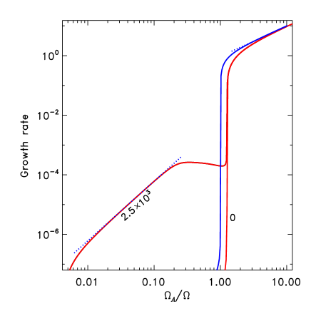
Figure 1: The growth rates normalized with the rotation rate for the kink-type instability of an equatorsymmetric toroidal field in a sphere, here with $\mathrm{Pm}=5\cdot 10^{-3}$, (see Kitchatinov & Rüdiger 2008). The two red lines are for $\rm q=0$ (right) and the solar value $\rm q=2500$ (left). The blue line gives the limits for both $g=0$ and $\chi\to\infty$.

For liquid sodium the Roberts number is small, $\rm q=10^{-3}$. The neglect of the thermal diffusion is thus fully realistic for MHD experiments in the laboratory. It is also realistic in stellar physics if the scenario of decaying fossil magnetic fields is considered. Moss (2003) finds poloidal fields of order 1000 G surviving in the inner radiation zones after the Hayashi track. Only after a short time, differential rotation produces the toroidal field component which tends to dominate the poloidal fields. The resulting Maxwell stress suppresses the differential rotation after the Alfvén travel time of the poloidal field unless the toroidal field becomes unstable. It seems to be clear that in order to be effective, the growth rate of the instability must be of order of the rotation rate rather than orders of magnitudes smaller.

The resulting instabilities form a nonaxisymmetric pattern of flow and field which transports both angular momentum and chemicals like lithium. We are interested in the possibility to express these fluxes by the gradients of mean quantities. The angular momentum flux for rigid rotation in our simplified model proves to be very small. It is thus reasonable to express the angular momentum transport by an eddy viscosity $\nu_{\rm T}$ and also to express the flux of chemicals by an eddy diffusivity $D_{\rm T}$. The amplitudes of the transport parameters are computed by nonlinear numerical simulations.

2 Astrophysical motivations

There is a variety of astrophysical applications. Only some of them are discussed in the present paper.

2.1 Rigid rotation in the solar interior

We know from the results of the helioseismology that the solar radiative interior rotates rigidly. This is insofar surprising as the microscopic viscosity with $\nu\lower 1.72218pt\hbox{$\;\buildrel<\over{\scriptstyle\sim}\;$}10\ {\rm cm}^{2}/{\rm s}$ of the hot solar plasma yields a diffusion time of more than $10^{13}$ yr so that any initial rotation law (which certainly existed) should be still existing without any other influence. One needs effective viscosities of $10^{5}\ {\rm cm}^{2}/{\rm s}$ to explain the decay of an initial rotation law within the lifetime of the Sun (see also Yang & Bi 2006). Future results of asteroseismology will show how general this statement is. Also the inclusion of the angular momentum transport by a poloidal magnetic field subject to differential rotation needs for the explanation of the solar spin-down the increase of the microscopic viscosity by a few orders of magnitude (Rüdiger & Kitchatinov, 1996). We have to test whether the angular momentum transport by magnetic instabilities of fossil magnetic fields is strong enough to produce the quasi-solid inner rotation of the Sun.

2.2 Diffusion of chemical elements

The lithium at the surface of cool MS stars decays with a timescale of 1 Gyr. It is burned at temperatures in excess of $2.6\times 10^{6}$ K which exists about 40.000 km below the base of the convection zone. There must be a diffusion process through this layer to the location of the burning temperature. Hence, we have to look for a slow process which, however, is only one or two orders of magnitude faster than the molecular diffusion. The molecular diffusion at the bottom of the solar convection zone results as $D_{\rm micro}\simeq 30$ cm²/s (Barnes, Charbonneau & MacGregor, 1999) which must be increased to about $10^{3}$ cm²/s as the consequence of a hypothetical instability. Note the smallness of this quantity: the plasma velocities for such a diffusion coefficient are by many orders of magnitude smaller than the convective velocities of about 100 m/s at the bottom of the convection zone.

There is thus a good motivation to look for a mechanism with a diffusion coefficient $D_{\rm T}>D_{\rm micro}$ but forming a turbulent Schmidt number with

$${\rm Sc}=\frac{\nu_{\rm T}}{D_{\rm T}}\gg 1$$ (3)

(see Zahn 1992). The expressions formulated by Eggenberger, Maeder & Meynet (2005) on the basis of the ‘Tayler-Spruit’ dynamo scenario lead for a toroidal magnetic field of about 100 Gauss to $\rm Sc\simeq 100$ (where the turbulent magnetic diffusivity has been used as the value for $D_{\rm T}$). This is a reasonable value for the Schmidt number. It is doubtful, however, that a toroidal field of 100 Gauss is unstable. For the upper part of the solar radiative core we found 600 Gauss as the minimum amplitude of a toroidal field to become unstable under the presence of the actual rotation rate, density stratification and diffusion processes (Kitchatinov & Rüdiger, 2008). A dynamo action could not be confirmed so far (Zahn, Brun & Mathis, 2007; Gellert, Rüdiger & Elstner, 2008).

Considering the transport processes in the radiative interior of massive (15 $M_{\odot}$) MS stars on the basis of analytic expressions by Spruit (2002), Maeder & Meynet (2003, 2005) computed viscosities up to $10^{13}\ {\rm cm}^{2}/{\rm s}$ for a rotational velocity of 300 km/s. The resulting diffusion time is only a few 100 yr. An extreme chemical mixing is the immediate consequence. With similar expressions Yoon, Langer & Norman (2006) present evolutionary models of rotating stars with different metalicities.

Angular momentum transporters could be Maxwell stress by both poloidal fields ($B_{R}$) and toroidal fields ($B_{\phi}$) which are connected by the differential rotation. If the Maxwell stress can be expressed by an effective viscosity and a very similar expression is used for chemical diffusion processes then the material mixing becomes so strong that the resulting evolution models are incompatible with observations. Brott et al. (2008) demonstrate that the corresponding chemical mixing in massive stars must even be neglected to understand the observations.

Note that the material mixing only results by the action of the kinetic part of the momentum transport tensor rather than by its magnetic part so that the diffusion tensor can be approximated by

$$D_{ij}\simeq\frac{1}{2}\tau_{\rm corr}\ \langle u_{i}^{\prime}(\mbox{\boldmath$x$},t)u_{j}^{\prime}(\mbox{\boldmath$x$},t)\rangle$$ (4)

(for details see Rüdiger & Pipin 2001). There is no magnetic influence in the diffusion equation except the magnetic suppression of the correlation tensor of the fluctuations.

If the correlation time of the instability scales with its growth time then the coefficient of the diffusion of chemicals can simply be written as

$$D_{\rm T}\simeq\frac{{\langle u_{R}^{\prime 2}\rangle}}{\gamma}.$$ (5)

For strong fields one can estimate the growth rate $\gamma\simeq{\it\Omega}$ (see below). Inserting numbers of the solar tachocline ($D_{\rm T}\simeq 10^{3}$ cm²/s, ${\it\Omega}\simeq 10^{-6}$ s^-1) leads to $u_{R}^{\prime}$ of order 0.1 cm/s. It is not easy to produce such a weak turbulence intensity in radial direction. The idea is that the stable density stratification below the convection zone suppresses the vertical turbulence component so that a highly anisotropic turbulence field evolves (Vincent, Michaud & Meneguzzi, 1996; Toqué, Lignières & Vincent, 2006). It has been shown, however, that due to the stellar rotation even a strictly horizontal flow pattern obtains radial components which are able to transport chemicals through the layer below the convection zone (Rüdiger & Pipin, 2001). The result is that the Li depletion becomes anticorrelated with the (rapid) stellar rotation or – with other words – the fast rotators should possess the highest surface concentrations of lithium. This consequence of the rotational quenching of the turbulence has indeed been found in the Pleiades cluster (Xing, Shi & Wei, 2007). Such a rotation-lithium correlation, however, could also be the consequence of the rotational quenching of the TI which is considered in the present paper.

3 Magnetic Taylor-Couette flow

3.1 The model

A Taylor-Couette container is considered confining a toroidal magnetic field with given amplitude at the cylinders rotating with different rotation rates (see Fig. 2). In order to simulate the situation at the bottom of the convection zone (or even at its top) the gap between the cylinders is considered as small. The outer radius is $R_{\mathrm{out}}$ and the inner radius is $R_{\mathrm{in}}$.

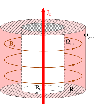
Figure 2: Two concentric cylinders with radii $R_{\mathrm{in}}$ and $R_{\mathrm{out}}$ rotate with ${\it\Omega}_{\rm in}$ and ${\it\Omega}_{\rm out}$. $B_{\phi}$ is the given toroidal magnetic field produced by axial currents inside and outside the inner cylinder.

The fluid confined between the cylinders is assumed to be incompressible with uniform density and dissipative with kinematic viscosity $\nu$ and magnetic diffusivity $\eta$. Derived from the conservation law of angular momentum the angular velocity of the rotation is

$${\it\Omega}=a+\frac{b}{R^{2}}$$ (6)

with

$$a=\frac{\mu_{\Omega}-\hat{\eta}^{2}}{1-\hat{\eta}^{2}}{\it\Omega}_{\rm in},\qquad b=\frac{1-\mu_{\Omega}}{1-\hat{\eta}^{2}}R_{\mathrm{in}}^{2}{\it\Omega}_{\rm in},$$ (7)

where

$$\hat{\eta}=\frac{R_{\rm{in}}}{R_{\rm{out}}},\qquad\mu_{\Omega}=\frac{{\it\Omega}_{\rm{out}}}{{\it\Omega}_{\rm{in}}}.$$ (8)

${\it\Omega}_{\rm in}$ and ${\it\Omega}_{\rm out}$ are the imposed rotation rates of the inner and outer cylinders. After the Rayleigh stability criterion the flow is hydrodynamically stable for $\mu_{\Omega}>\hat{\eta}^{2}$, i.e. $\mu_{\Omega}>0.25$ for $\hat{\eta}=0.5$. We are only interested in hydrodynamically stable regimes so that $\mu_{\Omega}>\hat{\eta}^{2}$ should always be fulfilled. Rotation laws with ${\rm d}{\it\Omega}/{\rm d}R<0$ are described by $\mu_{\Omega}<1$; $\mu_{\Omega}=1$ gives rigid rotation.

Also the magnetic profiles are restricted. The solution of the stationary induction equation without inducing flow reads

$$B_{\phi}=AR+\frac{B}{R}.$$ (9)

(in cylindric geometry. $A$ and $B$ are the fundamental quantities; $A\cdot R$ corresponds to a uniform axial current ($I=2A/\mu_{0}$) everywhere within $R<R_{\rm out}$, and $B/R$ corresponds to an additional current only within $R<R_{\rm in}$. The fields with $A=0$ are called the current-free solutions (current-free between the cylinders). Both terms in (9) are responsible for their own instability where one of them only exists in combination with differential rotation.

In analogy with $\mu_{\Omega}$ it is useful to define the quantity

$$\mu_{B}=\frac{B_{\rm{out}}}{B_{\rm{in}}},$$ (10)

measuring the variation in $B_{\phi}$ across the gap. Here we shall consider mainly fields which are rather uniform in radius, i.e. $\mu_{B}\simeq 1$. It is $B=R_{\rm in}R_{\rm out}A$ for this choice so that both parts of (9) are involved. The condition $A=0$ leads to profiles with $\mu_{B}=0.5$, and the condition $B=0$ leads to $\mu_{B}=2$ both for our standard case $\hat{\eta}=0.5$. After the stability criterion for toroidal fields against axisymmetric perturbations one finds stability of profiles with $0\leq\mu_{B}\ \leq 1/\hat{\eta}$ (see Shalybkov 2006). The magnetic fields discussed in the present paper are thus stable against disturbances with $m=0$ (see below).

In the following we shall fix $\mu_{B}=1$ but the rotation law and the magnetic Prandtl number

$$\mathrm{Pm}=\frac{\nu}{\eta}.$$ (11)

are varied. If the results shall be applied to stellar convection zones or e.g. to the fields in galaxies the magnetic Prandtl number must be replaced by its turbulent value.

3.2 The equations

The dimensionless incompressible MHD equations are

$${\rm Re}\frac{\partial\mbox{\boldmath$u$}}{\partial t}+{\rm Re}(\mbox{\boldmath$u$}\cdot\nabla)\mbox{\boldmath$u$}=-\nabla P+\Delta\mbox{\boldmath$u$}+{\mathrm{Ha}^{2}}\mathop{\rm rot}\nolimits\mbox{\boldmath$B$}\times\mbox{\boldmath$B$},$$

$${\rm Rm}\frac{\partial\mbox{\boldmath$B$}}{\partial t}=\Delta\mbox{\boldmath$B$}+{\rm Rm}\mathop{\rm rot}\nolimits(\mbox{\boldmath$u$}\times\mbox{\boldmath$B$}),$$ (12)

with $\mathop{\rm div}\nolimits{\mbox{\boldmath$u$}}=\mathop{\rm div}\nolimits{\mbox{\boldmath$B$}}=0$ and with the Hartmann number

$$\mathrm{Ha}=\frac{B_{\rm in}R_{0}}{\sqrt{\mu_{0}\rho\nu\eta}}.$$ (13)

$R_{0}=\sqrt{R_{\mathrm{in}}(R_{\mathrm{out}}-R_{\mathrm{in}})}$ is used as the unit of length, $\eta/R_{0}$ as the unit of velocity and $B_{\rm in}$ as the unit of the magnetic fields. Frequencies including the angular velocity ${\it\Omega}$ of the rotation are normalized with the rotation rate ${\it\Omega}_{\rm in}$. The Reynolds number $\mathrm{Re}$ is defined as

$$\mathrm{Re}=\frac{{\it\Omega}_{\rm in}R_{0}^{2}}{\nu},$$ (14)

and the magnetic Reynolds number as $\mathrm{Rm}=\mathrm{Pm}\cdot\mathrm{Re}$. The Lundquist number is simply $\rm S=\mathrm{Ha}\sqrt{\mathrm{Pm}}$.

The boundaries are assumed as impenetrable and stress-free and as perfect conductors.

The solutions of the linear equations are free to an arbitrary real parameter of any sign. We thus cannot know the sign of the flow and/or the field. However, for quadratic expressions such as the correlation tensor or the electromotive force we can compute the sign as all the solutions are multiplied with one and the same parameter.

Let us apply this idea to the angular momentum transport

$$T_{R}=\langle u_{R}^{\prime}u_{\phi}^{\prime}-\frac{1}{\mu_{0}\rho}B_{R}^{\prime}B_{\phi}^{\prime}\rangle.$$ (15)

The averaging procedure is thought to be an integration over the azimuth $\phi$. The question we shall answer is whether $T_{R}>0$ for ${\rm d}{\it\Omega}/{\rm d}R<0$ and $T_{R}<0$ for ${\rm d}{\it\Omega}/{\rm d}R>0$. If this is true then the angular momentum flows towards the minimum of the angular velocity and one can introduce an eddy viscosity $\nu_{\rm T}$, i.e.

$$T_{R}=-\nu_{\rm T}R\frac{{\rm d}{\it\Omega}}{{\rm d}R}$$ (16)

with positive $\nu_{\rm T}$. The sign of $\nu_{\rm T}$ can be computed with the linear theory. We have computed this quantity with both linear and nonlinear approximations. With the linear theory bifurcation diagrams for various rotation laws and magnetic Prandtl numbers are established and it is shown that the angular momentum (kinetic plus magnetic) flows opposite to the gradient of the angular velocity. It is thus possible in this case to define via (16) an eddy viscosity on the basis of the Tayler instability. With the nonlinear simulations the amplitude of this eddy viscosity is computed.

With $U=\langle u_{R}^{\prime 2}\rangle$ the ratio of $\nu_{\rm T}$ and $D_{\rm T}$ results to

$${\rm Sc}=\frac{1}{q}\frac{T_{R}}{U}$$ (17)

with $q=-{\rm d}{\rm log}{\it\Omega}/{\rm d}{\rm log}R$. Without Maxwell stress this quantity is certainly of order unity but it can acquire much higher values if the magnetic-induced angular momentum transport dominates.

4 Marginal instability

In the linear approximation the solutions can be found in form of normal modes in accord to

$$F=F(R){\rm e}^{{\rm i}(kz+m\phi+\omega t)}.$$ (18)

Here $m$ is the azimuthal quantum number of the resulting cell pattern. For instabilities the growth rate $\gamma=-\Im(\omega)$ must be positive and the neutral lines are defined by $\gamma=0$. In this Section the neutral lines for the magnetic instability with $m=1$ are presented. The wave number $k$ is optimized so that the resulting Reynolds number becomes a minimum for given Hartmann number.

Figure 3: The lines of neutral instability for $A=0$ (AMRI). The curves are marked with their magnetic Prandtl numbers. The toroidal fields are current-free between the (conducting) cylinders. It is $\mu_{B}=\hat{\eta}=0.5$, $\mu_{\Omega}=0.5$.

4.1 The maps of neutral instability

Let us start with the phenomenon that even current-free toroidal fields can become unstable if they are subject to differential rotation. For $\hat{\eta}=0.5$ follows $\mu_{B}=0.5$ for the magnetic profile, and the differential rotation may be as weak as $\mu_{\Omega}=0.5$ simulating a (galactic) rotation law ${\it\Omega}\propto 1/R$. The map for neutral instability of this interaction for various magnetic Prandtl numbers is given in Fig. 3. The disturbances with $m=1$ can grow although the magnetic field or the differential rotation alone are stable. We have called this phenomenon as Azimuthal Magnetorotational Instability (AMRI, see Rüdiger et al. 2007, also Ogilvie & Pringle 1996). It is very characteristic for AMRI that it disappears for rigid rotation but also if the (differential) rotation becomes too strong. This is the reason why both lines of the marginal stability have the same positive slope.

Figure 4: The marginal-instability map for toroidal fields with $A\simeq B$ ($\mu_{B}=1$). Top: Rotation vs magnetic field. The AMRI domain and the TI domain are separated by a stable branch. Bottom: The stable branch between the AMRI domain and the TI domain corresponds to the line $\rm Mm=1$. It is $\mathrm{Pm}=1$, $\mu_{\Omega}=0.5$, $\hat{\eta}=0.5$.

An axial current ($I=2A$) is not necessary for AMRI. But the AMRI survives the addition of axial electric currents in the fluid conductor (i.e. $A\neq 0$). It also appears in the instability maps of toroidal fields with electric currents between the cylinders (Fig. 4). In this figure the results for $\mathrm{Pm}=1$ and for weak subrotation ($\mu_{\Omega}=0.5$) are given for almost homogeneous fields with $\mu_{B}=1$. For this magnetic profile both the coefficients $A$ and $B$ in Eq. (9) are finite. The characteristic AMRI domain only vanishes for magnetic profiles with $B=0$.

Without rotation the magnetic field alone is unstable for $\rm Ha\geq 150$ because of the action of the axial current. We shall call this domain of subAlfvénic rotation as the domain of the Tayler instability (TI). It also exists for $B=0$. The critical Hartmann number for vanishing rotation does not depend on Pm. In Fig. 4 two unstable domains with different growth rates exist. The growth rate is of order ${\it\Omega}$ in the TI domain but it is smaller in the AMRI domain (see below). Both domains are separated by a stability branch along the line $\rm Rm=Ha$ which disappears, however, for $\rm Pm>1$ (see Rüdiger et al. 2007). The AMRI domain in Fig. 4, of course, disappears for solid-body rotation.

Figure 5: Top: The rotational quenching of the TI for rigid rotation and for various Pm. The dashed line gives $\rm Mm=1$. Note that for $\rm Pm=1$ the rotational quenching of the magnetic instability is strongest. Bottom: TI is a subAlfvénic phenomenon. $\hat{\eta}=0.5$, $\mu_{B}=1$.

Note that the rotation basically stabilizes the instability (Pitts & Tayler, 1985). The faster the rotation the stronger fields remain stable. We must keep this effect in mind for stellar applications. Magnetic fields which are stable for fast rotation become unstable during the stellar evolution with its continuous spin-down. Also the magnetic Prandtl number influences the rotational quenching. One finds the main result already by comparing the instability maps for rigid rotation only. The magnetic Prandtl number has been varied by two orders of magnitudes in Fig. 5. It makes sense to interprete the results by means of the ‘mixed’ Reynolds number

$${\rm Rem}=\sqrt{{\mathrm{Re}\cdot\mathrm{Rm}}},$$ (19)

which by definition is symmetric in $\nu$ and $\eta$ as it is the Hartmann number. All fluids with the same product $\nu\cdot\eta$ have the same Rem and Ha. Consequently, the ratio of the mixed Reynolds number Rem and the Hartmann number Ha is a magnetic Mach number

$${\rm Mm}=\frac{\rm Rem}{\rm Ha},$$ (20)

in which the numerical values of viscosity and magnetic diffusivity do no longer appear. $\rm Mm>1$ means superAlfvénic rotation and $\rm Mm<1$ describes subAlfvénic rotation.

The rotational stabilization of the toroidal fields also depends on the form of the rotation law. It is weaker for subrotation and it is stronger for rigid rotation and for superrotation (Fig. 6). The trend is understandable as superrotation is the most stable rotation law in hydrodynamics. For given rotation rate the maximum field amplitudes which remain stable are much weaker for subrotation than for rigid rotation. With other words: rigid rotation stabilizes magnetic fields more effective than subrotation. For very fast rotators, however, the nonaxisymmetric instability is always suppressed. For superAlfvénic rotation ($\mathrm{Re}\gg\mathrm{Ha}$) the magnetic fields become stable also for rotation laws with negative shear.

Figure 6: The marginal-instability map for subrotation ($\mu_{\Omega}=0.5$), for rigid rotation ($\mu_{\Omega}=1$) and for superrotation ($\mu_{\Omega}=1.25$). The curve for $\mu_{\Omega}=0.5$ is taken from Fig. 4. It is $\mu_{B}=1$, $\mathrm{Pm}=1$, $\hat{\eta}=0.5$.

4.2 Growth rates

The growth rates $\gamma$ are the negative imaginary part of the frequency $\omega$ in Eq. (18). They are given (normalized with the rotation frequency of the inner cylinder) in the Fig. 7. The growth time in units of the rotation time can be obtained as $\tau_{\rm growth}/\tau_{\rm rot}=1/(2\pi\gamma)$. Hence, for $\gamma=1/2\pi=0.16$ the growth time equals the rotation time.

The growth rates in the TI domain of Fig. 4 are given in Fig. 7. They are much larger than 0.16 so that the growth time of the instability is smaller than the rotation period. Note the rotational quenching of the growth rates. As they are normalized with the inner rotation frequency, however, this is a formal effect. It means in Fig. 7 that the physical growth time (in units of the dissipation time) does not depend on the rotation rate but it grows linearly with the magnetic field (see Goosens, Biront & Tayler 1981).

Figure 7: The (normalized) growth rates for $\rm Pm=1$ (see Fig. 4). Top: the TI domain. The curves are marked with their Reynolds numbers. After multiplication with Re they are almost identical. Bottom: along the line $\rm Re=500$ of Fig. 4 (AMRI and TI).

Figure 7 (bottom) provides the comparison of the growth rates of TI with those of AMRI. The values are calculated along the line $\mathrm{Re}=500$ of Fig. 4. While the growth time of the AMRI remains slower than the rotation period the TI modes become faster and faster for growing magnetic amplitudes.

4.3 Magnetic limits

Figure 5 shows the limit of the subAlfvénic Tayler instability for rigid rotation but for various Pm in the Rem-Ha plane. One finds the Pm-dependence of the resulting magnetic Mach numbers as rather weak. For $\mathrm{Pm}>1$ the Rem are largest, i.e. for large Pm the rotational quenching is weak. It is stronger for $\mathrm{Pm}<1$ but it is strongest for $\mathrm{Pm}=1$ which is the favored application for all kinds of numerical simulations.

The stabilization of the toroidal magnetic fields against Tayler instability in rigidly rotating radiative stellar zones is now considered. From Fig. 5 we take the simple relation

$$\rm Mm\simeq 0.5.$$ (21)

Large Mm means weak rotational quenching of the instability which appears to be realized for $\mathrm{Pm}\neq 1$. If (21) is true then

$$B_{\phi}\lower 1.72218pt\hbox{$\;\buildrel>\over{\scriptstyle\sim}\;$}2\sqrt{\mu_{0}\rho}\ u^{*}$$ (22)

leads to instability, i.e.

$$B_{\phi}\,[{\rm Gauss}]>2\ u^{*}\,[{\rm cm/s}]$$ (23)

when the linear rotation velocity $u^{*}$ of the stellar interior is taken in cm/s. One thus needs more than 100 kGauss to get a marginal TI instability of toroidal fields in the rotating Sun. For Ap stars with their higher rotation velocities and higher mean densities even amplitudes of more than 10⁶ Gauss are necessary. Due to the stellar rotation large-scale toroidal fields remain stable up to this value. Note that Heger, Woosley & Spruit (2005) work with toroidal field amplitudes of $10^{4}$ Gauss. For hot MS stars with their extended radiative zones and a linear rotation rate of (say) 100 km/s the minimum magnetic amplitude for the Tayler instability is $10^{7}$ Gauss. This result only concerns to the fast Tayler instability with growth times shorter than the rotation period. By the action of high thermal diffusion in the radiative stellar cores also weaker toroidal fields can become unstable but with much larger growth times (see Fig. 1). Note that probably almost all rotating objects belong to the fast-rotating class with ${\rm Mm}>1$. For the exceptional case of galaxies whose inner toroidal fields can be observed, the relation ${\rm Mm}>1$ is true.

More calculations with smaller magnetic Prandtl numbers are needed to find the final results for the limits of the Tayler instability of toroidal fields in rapidly rotating stars. Of course, we can only speculate whether the obtained linear scaling also holds for very fast rotation. Already small deviations from the linear dependence in (21) would provide strongly different magnetic field amplitudes. On the other hand, the present results from the global theory of magnetic instability of toroidal fields in regions of high thermal diffusion find the rotational stabilization of TI as very effective. Because of the much weaker rotational quenching seen in Fig. 4 for the AMRI this sort of magnetic instability seems to be more important for stellar physics. We shall see that indeed this instability transports much more angular momentum than the TI. Note that the AMRI only exists under the presence of differential rotation.

Opposite to stars for galaxies we can measure their interior magnetic fields so that the magnetic Mach number is well-known. It is much larger than unity so that galaxies should be TI stable. However, because of their very high magnetic Prandtl number together with the particular galactic rotation law new calculations are needed in order to probe their stability.

5 The angular momentum transport

Gellert & Rüdiger (2008) have shown that the angular momentum transport anticorrelates with $\nabla{\it\Omega}$. A formulation as in (16) (‘diffusion approximation’) is indeed possible. One can show that the quantity $T_{R}$ vanishes for rigid rotation and it is linear in $\nabla{\it\Omega}$. It makes thus sense to define an eddy viscosity with a sofar unknown amplitude. In a linear theory a determination of the numerical value of the eddy viscosity is not possible. We thus start with nonlinear simulations for a container with $\hat{\eta}=0.5$, also to minimize the influence of the boundary conditions.

For the same reason the cylinder is regarded with a periodicity in the vertical coordinate $z$ set to $6(R_{\mathrm{out}}-R_{\mathrm{in}})$. We use the MHD Fourier spectral element code described by Fournier et al. (2004) and Gellert, Rüdiger & Fournier (2007). In this approach the solution is expanded in $M$ Fourier modes in the azimuthal direction. The resulting decomposition is a collection of meridional problems, each of which is solved using a Legendre spectral element method (see e.g. Deville, Fischer & Mund 2002). Either $M=8$ or $M=16$ Fourier modes are used, two or three elements in radius and twelve or eighteen elements in axial direction, resp. The polynomial order is varied between $N=8$ and $N=16$. With a semi-implicit approach consisting of second-order backward differentiation formula and third order Adams-Bashforth for the nonlinear forcing terms time stepping is done with second-order accuracy. At the inner and outer wall no-slip and perfect conducting boundary conditions are applied.

The Taylor-Couette flow (6) as initial flow and white noise for the initial magnetic field are used. Additionally applied is the toroidal field with $\mu_{B}=1$ as external field. The differential rotation is varied between $\mu_{\Omega}=0.3$ and $\mu_{\Omega}=1.5$. At these parameter values the field becomes unstable. In the linear regime only the Fourier mode $m=1$ grows exponentially. Already after roughly one rotation, when nonlinear effects become important, also higher modes appear. Though, the mode spectrum drops very quickly with increasing $m$. More than $99\%$ of the energy is contained within the first three modes. After only a few rotations all excited modes saturate and a steady-state is reached. The resulting fields are averaged in azimuthal direction and the nonaxisymmetric components are regarded as fluctuating quantities.

In accordance to Eq. (15) the angular momentum transport is calculated. Figure 8 shows for subrotation ($\mu_{\Omega}=0.5$, quasigalactic rotation law), $\mu_{B}=1,\mathrm{Pm}=1$ and a Hartmann number of $\mathrm{Ha}=250$ how $T_{R}$ depends on the magnetic Reynolds number. For $T_{R}$ its values in the center of the gap and averaged over $z$ are used. The angular momentum transport scales with $\mathrm{Rm}^{2}$ up to $\mathrm{Rm}=600$. The last two points do not follow this rule because the upper limit for the instability is approached. The differential rotation becomes too strong and suppresses the nonaxisymmetric magnetic instability equivalent to the results of the linear analysis (Fig. 4). Maxima as shown in Fig. 8 basically exist due to the limit of fast rotation which always exists for the nonaxisymmetric magnetic instability. In order to find the angular momentum transport of kink-type instabilities it is necessary to find this maximum and to compute the maxima for increasing magnetic fields (see Fig. 11, below). The question is how the maxima scale with increasing Ha. If they saturate for large Ha the characteristic angular momentum transport is known.

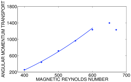
Figure 8: Values of $T_{R}$ (in the center of the gap) for superAlfvénic rotation for $\hat{\eta}=0.5,\ \mu_{\Omega}=0.5,\ \mu_{B}=1,\ \mathrm{Pm}=1$ and for fixed $\mathrm{Ha}=250$. The fitted parabola shows $T_{R}$ depending on $\mathrm{Rm}^{2}$. For too high $\mathrm{Rm}$ the instability is suppressed so that always a maximum exists for fixed Ha at a certain rotation rate.

All the nonlinear simulations demonstrate that the angular momentum transport $T_{R}$ scales linearly with ${\rm d}{\it\Omega}/{\rm d}R$ so that a characteristic eddy viscosity can be introduced. In the following, these eddy viscosities are calculated in the two instability domains shown in Fig. 4. The domain TI is characterized by subAlfvénic rotation and strong fields while in the AMRI domain the rotation is superAlfvénic. We shall find that AMRI produces much higher values of eddy viscosity rather than TI.

5.1 Slow rotation

We start to consider the instability domain of subAlfvénic rotation. In the TI area of Fig. 4 for a small Reynolds number ($\mathrm{Re}=30$) and for various Hartmann numbers exceeding $\mathrm{Ha}=180$ the torque $T_{R}$ and the eddy viscosity are calculated. The eddy viscosity is normalized with the molecular viscosity so that the results are fully general. The normalized eddy viscosities prove to be very small. Note the saturation for increasing Hartmann numbers (Fig. 9). We found the small values of the eddy viscosity as characteristic for the considered combination of strong fields and slow rotation.

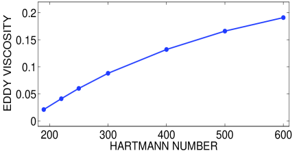
Figure 9: Viscosities $\nu_{\rm T}/\nu$ for subAlfvénic rotation and for $\mu_{\Omega}=0.5$. It is $\mu_{B}=1$, $\mathrm{Re}=30$, $\hat{\eta}=0.5$, $\mathrm{Pm}=1$.

5.2 Rapid rotation

The eddy viscosity is now calculated as a function of the Reynolds number of rotation for the same set of parameters used in Fig. 8. All these models belong to the domain AMRI in the instability map of Fig. 4. The results are plotted in Fig. 10. For $\nu_{\rm T}/\nu$ a scaling with $\mathrm{Rm}^{2}$ is found in opposition to the $\mathrm{Rm}^{-1}$ scaling by Maeder & Meynet (2005). Due to the rotational quenching of the instability a maximum exists characteristic for the given magnetic field. The resulting viscosities $\nu_{\rm T}/\nu$ are much higher than for subAlfvénic rotation but they do not exceed the value of (say) 25. Figure 11 shows the results of calculations of maximum values for $\nu_{\rm T}/\nu$ for increasing magnetic amplitudes. Also the Reynolds numbers belonging to the maximum viscosity are given. We find a saturation of the ratio $\nu_{\rm T}/\nu$ for strong magnetic fields. The eddy viscosity exceeds the microscopic viscosity not more than by a factor of 100. The same procedure must be applied to the other possible magnetic profiles in order to confirm the existence of the magnetic saturation suggested by Fig. 11. The existence of the maximum of $\nu_{\rm T}/\nu$ for fixed magnetic field as shown in Fig. 10 seems to be clear. The existence of the saturation for stronger magnetic fields must be checked by further calculations.

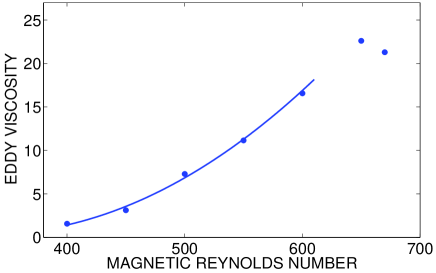
Figure 10: The same as in Fig. 8 but for $\nu_{\rm T}/\nu$. Note the existence of the maximum value due to the rotational stabilization.

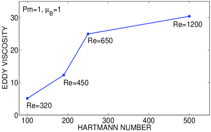
Figure 11: The maximum $\nu_{\rm T}/\nu$ for various Hartmann numbers, $\mathrm{Pm}=1$. The curves are marked with the Reynolds number where the eddy viscosity is largest. The normalized eddy viscosity seems to saturate for strong magnetic fields. Note that always $\rm Mm>1$.

We have also computed the expression (5) for turbulent diffusion with growth rates $\gamma$ taken from the initial growth phase of the instability. which unfortunately is a very simple approximation. Therefore, the results do not have the same accuracy as the viscosity values. Values are approximately one order of magnitude below the eddy viscosity leading to high Schmidt numbers ${\rm Sc}\approx 30$ (Fig. 12). We do not find a strong dependence on the magnetic field strength. It seems to be true that the kink-type instability for toroidal fields produces medium viscosity values by Maxwell stress and small diffusivity values by Reynolds stress. So far we cannot find a remarkable influence of the amplitude of the toroidal field on the resulting Schmidt number.

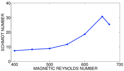
Figure 12: The Schmidt number ${\rm Sc}=\nu_{\rm T}/D_{\rm T}$ vs. Reynolds number Rm for $\mathrm{Ha}=250$ and $\mathrm{Pm}=1$.

6 Main results

The stability of toroidal magnetic fields is considered in cylindric geometry. The toroidal fields can be imagined as resulting from the interaction of weak poloidal fields with differential rotation. For $\mathrm{Rm}\gg 1$ it makes sense to consider the stability for the MHD system under neglect of the poloidal field. In the present paper the stability/instability of stationary toroidal fields against nonaxisymmetric perturbations with $m=1$ under the presence of rigid or differential rotation is discussed.

We have shown that under the influence of a rigid rotation the marginal instability of toroidal fields is basically suppressed. Note that the suppression is strongest for $\mathrm{Pm}=1$ and becomes weaker for any other value of Pm. For differential rotation the situation is more complicated. For superrotation (${\rm d}{\it\Omega}/{\rm d}R>0$) the suppression is even stronger than for rigid rotation, while for subrotation (${\rm d}{\it\Omega}/{\rm d}R<0$) it also exists but only for very fast rotation. These results are understandable because too strong differential rotation always disturbs nonaxisymmetric magnetic configurations.

For radiative zones the kink-type instability can be considered as an angular momentum transporter. The angular momentum transport vanishes for solid-body rotation and the angular momentum is always transported opposite to the gradient of the angular velocity so that a ‘diffusion approximation with an eddy diffusivity makes sense. The eddy viscosity resulting from our simulations exceeds the microscopic viscosity not more than by 1–2 orders of magnitudes. The truth of this statement bases on the existence of the magnetic saturation of the maximum viscosity values presented in Fig. 11. Further simulations are needed to confirm this finding.

If angular momentum is transported and the transport is not completely magnetic then also the considered fluid is continously mixed. For strong mixing the stellar evolution would too strongly be affected (see Brott et al. 2008), hence the mixing induced by magnetic instability must remain weak. Also the lithium observations of solar-type stars are not understandable without the existence of a rather mild turbulence beneath the stellar convection zones. One may argue that the mixing is due to the Reynolds stress while the angular momentum transport is mainly due to the Maxwell stress. If the Maxwell stress dominates the Reynolds stress then the general transport problem formulated by Zahn (1992) is solved. We indeed find such a tendency with nonlinear simulations. The eddy viscosity exceeds the diffusion coefficient by one or two orders of magnitude. Very similar results are reported by Carballido, Stone & Pringle (2005) and Johansen, Klahr & Mee (2006) for simulations of the magnetorotational instability.

It is an open question whether the dominance of eddy viscosity over turbulent diffusion can even be stronger. Figure 12 does not lead in this direction. More simulations with different magnetic profiles and/or with smaller magnetic Prandtl numbers must show how many orders the magnetic-induced angular momentum transport exceeds the diffusion of chemicals.

Note that the values derived with our model – in particular the value for the diffusion coefficient (5) – are maximum values as the suppressing action of the density stratification and the destabilizing action of the microscopic thermal diffusion is still neglected. Also the restriction to magnetic Prandtl number of order unity and the consideration of a special magnetic profile are still serious limitations.

References

- Acheson (1978) Acheson D. J., 1978, Phil. Trans. Roy. Soc., 289, 459
- Barnes, Charbonneau & MacGregor (1999) Barnes G., Charbonneau P., MacGregor K. B., 1999, ApJ, 511, 466
- Brott et al. (2008) Brott I., Hunter I., Anders P., Langer N., 2008, astro-ph/0709.0874
- Carballido, Stone & Pringle (2005) Carballido A., Stone J. M., Pringle J. E., 2005, MNRAS, 358, 1531
- Deville, Fischer & Mund (2002) Deville M. O., Fischer P. F., Mund E. H., 2002, High Order Methods for Incompressible Fluid Flow, Cambridge University Press
- Eggenberger, Maeder & Meynet (2005) Eggenberger P., Maeder A., Meynet G., 2005, A&A, 440, L9
- Fournier et al. (2004) Fournier A., Bunge H.-P., Hollerbach R., Vilotte J.-P., 2004, Geophys. J. Int., 156, 682
- Gellert & Rüdiger (2008) Gellert M., Rüdiger G., 2008, AN, 329, 709
- Gellert, Rüdiger & Fournier (2007) Gellert M., Rüdiger G., Fournier A., 2007, AN, 328, 1162
- Gellert, Rüdiger & Elstner (2008) Gellert M., Rüdiger G., Elstner D., 2008, A&A, 479, L33
- Goossens, Biront & Tayler (1981) Goossens M., Biront D., Tayler R. J., 1981, Ap&SS, 75, 521
- Heger, Woosley & Spruit (2005) Heger A., Woosley S. E., Spruit H. C., 2005, ApJ, 626, 350
- Johansen, Klahr & Mee (2006) Johansen A., Klahr H., Mee A. J., 2006, MNRAS, 370, L71
- Kitchatinov & Rüdiger (2008) Kitchatinov L. L., Rüdiger G., 2008, A&A, 478, 1
- Maeder & Meynet (2003) Maeder A., Meynet G., 2003, A&A, 411, 543
- Maeder & Meynet (2005) Maeder A., Meynet G., 2005, A&A, 440, 1041
- Moss (2003) Moss D., 2003, A&A, 403, 693
- Ogilvie & Pringle (1996) Ogilvie G. I., Pringle J. E., 1996, MNRAS, 279, 152
- Pitts & Tayler (1985) Pitts E., Tayler R. J., 1985, MNRAS, 216, 139
- Rüdiger & Kitchatinov (1996) Rüdiger G., Kitchatinov L. L., 1996, ApJ, 466, 1078
- Rüdiger & Pipin (2001) Rüdiger G., Pipin V. V., 2001, A&A, 375, 149
- Rüdiger et al. (2007) Rüdiger G., Hollerbach R., Schultz M., Elstner D., 2007, MNRAS, 377, 1481
- Shalybkov (2007) Shalybkov D., 2006, Phys. Rev. E, 73, 016302
- Spruit (2002) Spruit H. C., 2002, A&A, 381, 923
- Tayler (1957) Tayler R. J., 1957, Proc. Phys. Soc. B, 70, 31
- Tayler (1973) Tayler R. J., 1973, MNRAS, 161, 365
- Toqué, Lignières & Vincent (2006) Toqué N., Lignières F., Vincent A., 2006, GAFD, 100, 85
- Vandakurov (1972) Vandakurov Yu. V., 1972, SvA, 16, 265
- Vincent, Michaud & Meneguzzi (1996) Vincent A., Michaud G., Meneguzzi M., 1996, Phys. Fluid, 8, 1312
- Xing, Shi & Wei (2007) Xing L.-F., Shi J.-R., Wei J.-Y., 2007, New Astronomy, 12, 265
- Yang & Bi (2006) Yang W. M., Bi S. L., 2006, A&A, 449, 1161
- Yoon, Langer & Norman (2006) Yoon S.-C., Langer N., Norman C., 2006, A&A, 460, 199
- Zahn (1992) Zahn J.-P., 1992, A&A, 265, 115
- Zahn, Brun & Mathis (2007) Zahn J.-P., Brun A. S., Mathis S., 2007, A&A, 474, 145