Phase-resolved Faraday rotation in pulsars

Abstract

We have detected significant Rotation Measure variations for 9 bright pulsars, as a function of pulse longitude. An additional sample of 10 pulsars showed a rather constant RM with phase, yet a small degree of RM fluctuation is visible in at least 3 of those cases. In all cases, we have found that the rotation of the polarization position angle across our 1.4 GHz observing band is consistent with the $\lambda^{2}$ law of interstellar Faraday Rotation. We provide for the first time convincing evidence that RM variations across the pulse are largely due to interstellar scattering, although we cannot exclude that magnetospheric Faraday Rotation may still have a minor contribution; alternative explanations of this phenomenon, like erroneous de-dispersion and the presence of non-orthogonal polarization modes, are excluded. If the observed, phase-resolved RM variations are common amongst pulsars, then many of the previously measured pulsar RMs may be in error by as much as a few tens of rad m^-2.

1 Introduction

Radio pulsars are generally highly polarised sources, and the propagation of their radiation through the magneto-ionised interstellar medium (ISM) is affected by Faraday rotation. Measurement of the rotation measure (RM), combined with the dispersion measure (DM) for each pulsar, provides a good estimate of the average magnetic-field strength in the direction of the line of sight to many of the known pulsars. With the high sensitivity and broad bandwidths of current observing instruments, it is possible to accurately measure RMs within a single band, thus avoiding calibration issues of observing with different receivers in different bands. Furthermore, observing pulsars with high temporal resolution allows RM measurements at different pulse longitudes, provided the signal to noise ratio of the linearly polarised component is sufficient.

Ramachandran et al. (2004) presented a phase-resolved RM analysis for PSR B2016+28. In an attempt to explain the variation in RM by $\pm 15$ rad m^-2 across the pulse profile, they conducted a single-pulse analysis of the polarization. They found that there are clearly two, almost orthogonal polarization modes across the pulse profile, with slightly different spectra (as also postulated in Karastergiou et al. 2005 and demonstrated in Smits et al. 2006). Superposition of these modes results in a net change in the polarization position angle with frequency, leading to the measurement of a variable RM across the pulse. Although the effect measured in their study rotates the position angle (PA) with frequency, they concluded that it is not Faraday rotation intrinsic to the pulsar magnetosphere. The authors clearly demonstrate that for PSR B2016+28 the position angle does not have a quadratic dependence on wavelength: i.e. $\Delta{\rm PA}={\rm RM}\cdot\lambda^{2}$.

A very recent work by [12] showed that even small amounts of interstellar scattering can significantly deform the steep features of PA profiles (e.g. orthogonal mode jumps), and can provide a simple explanation for the RM variations observed by Ramachandran et al. The latter is caused by the frequency dependence of the scattering constant, which causes a frequency-dependent amount of polarised intensity to be transfered from a given phase bin to later phases. Regions where the PA profile has a steep gradient are worst affected, since it is at those phases where the scattered portion of the polarised intensity has the most impact on the shape of the PA profile: flat profiles can only stay flat, but the kinks and wiggles in PA profiles will be distorted by the redistribution of the polarised intensity. Hence, Karastergiou noted that the polarization of core components, where PA profiles are steepest, is affected the most. The author concluded that scattering can smear orthogonal polarization modes so that they appear slightly less “orthogonal”.

In this paper we concentrate on pulsars for which we have recently published RM values (e.g. Noutsos et al. 2008). Our aim is not only to fit for pulse phase–resolved RMs, as was done in Ramachandran et al., but to closely investigate whether the polarization position angles obey $\lambda^{2}$ fits. We investigate the possible causes for this particular PA frequency dependence and discuss implications on RM measurements performed using different techniques.

2 Observations and data analysis

The data used in our analysis were collected with the Parkes 64-m radio telescope during two observing periods: in 2004, August 31 to Septemeber 1, and in 2006, August 24 to 27. We observed at the frequency band of the 20cm H-OH receiver, installed at the focus cabin of the Parkes telescope. The receiver is equipped with a pair of orthogonal, linear feeds that are sensitive to polarised emission with an equivalent system flux density of 43 Jy at 20cm (Johnston 2002). The 2004 data were observed with a central frequency of 1.375 GHz and 256 MHz bandwidth, while in 2006 we observed with a central frequency of 1.369 GHz and 256 MHz bandwidth.

The wide-band correlator (WBC) back end that was used in both observations is capable of splitting the available bandwidth into 1,024 frequency channels, on each of four polarizations, $I$, $Q$, $U$ and $V$, and producing 10-s de-dispersed pulse subintegrations with up to 2,048 phase bins across the pulse profile.

In Noutsos et al. (2008), we outline the method used to derive a single RM value for each pulsar we observed. Here, we performed the same analysis of the polarised emission in each longitude bin, across the total pulse width. Our aim was to produce RM profiles as a function of longitude for each observed pulsar. Prior to our analysis, the raw data from the WBC were subjected to the necessary process of RFI mitigation and polarization calibration. We processed the calibrated data using the PSRCHIVE software package [7].

It is expected that the plane of linearly polarised emission will be rotated by the magnetised ISM it traverses on its way to the Earth: this is the well-known interstellar Faraday effect. The amount of rotation, $\Delta{\rm PA}$, for a given pulsar should be constant for a specific frequency but scales as $1/f^{2}$ across the observing band. By definition, the rotation between frequency $f$ and infinite frequency gives the PA at frequency $f$:

$${\rm PA}=c^{2}{\rm RM}\frac{1}{f^{2}}$$ (1)

Since the RM is a physical property of the ISM, it is expected to be constant for a given ISM configuration between the pulsar and the Earth. Its value depends on the magnitude and direction of the magnetic field, $\boldsymbol{B}$, along the propagation path of the polarised emission, $C$; the free-electron density, $n_{e}$, along $C$, and the length of $C$; it is given by the path integral

$${\rm RM}\propto\int_{C}n_{e}\boldsymbol{B}\cdot d\boldsymbol{l}$$ (2)

where $d\boldsymbol{l}$ is directed from the pulsar to the Earth.

Apart from the pulsar distance, none of the remaining physical quantities, on which RM depends, are directly measurable. However, given a finite observing bandwidth, one can derive RM by fitting the PA across the band with the quadratic function of equation 1. The PA of each bin $i$ in each frequency channel $j$ was calculated as ${\rm PA}_{i,j}=0.5\arctan{(U_{i,j}/Q_{i,j})}$.

Having previously developed the software capable of such quadratic fits (see Noutsos et al. 2008 for details), we performed bin-wise fitting across the longitude range inside the pulse and derived a value of RM for each individual longitude bin. In order to increase the s/n per frequency channel, $j$, before fitting across the whole available bandwidth we averaged the frequency channels by a factor 16. For a single averaging factor, as is the case in this analysis, only the statistical error on each RM value can be calculated, and the fitting routine gives the best integer RM for each bin. Finally, we plotted pulse profiles of the total flux density, the linear- and circular-polarization components, and the PA and RM profiles across the pulse; we only plotted significant PA values with ${\rm s/n}>3.5$ and RM values with $\sigma_{\rm RM}<5$ rad m^-2.

3 Results

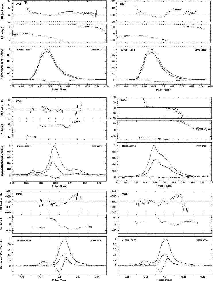
Figure 1: Profiles of the RM as a function of pulse longitude (top panels), for 9 pulsars, observed at 20 cm with the Parkes telescope, that exhibit large RM variations across their pulse profile. The respective year of observation is shown at the top-left corner of each pulsar’s RM profile. For two pulsars, namely the Vela pulsar and PSR J1326$-$5859, we had data from two observing sessions, in 2004 and 2006. The RM for each longitude bin was calculated from a quadratic fit to the PAs of that bin across the frequency band. Only RM values with $\sigma_{\rm RM}<5$ rad m^-2 are shown. The horizontal, gray line across the RM profiles shows the published RM value for each pulsar. The middle panels show the phase-resolved PA profiles, calculated from the integrated Stokes profiles, $Q$ and $U$, across the respective frequency band. For each longitude bin, the PA was calculated as ${\rm PA}=0.5\arctan(U/Q)$. Only PAs corresponding to linear polarisation with ${\rm s/n}>3.5$ are shown. The bottom panels show the profile of the total flux density (solid lines) and the linear (dashed lines) and circular (dotted lines) polarization flux for each pulsar.

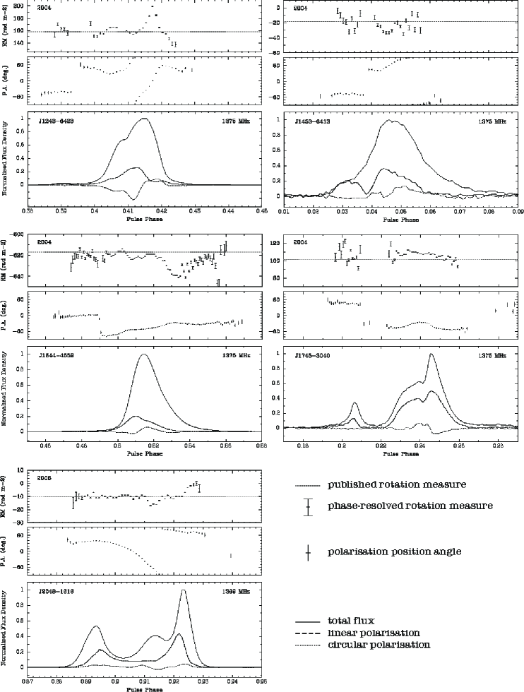
Figure 1: Continued

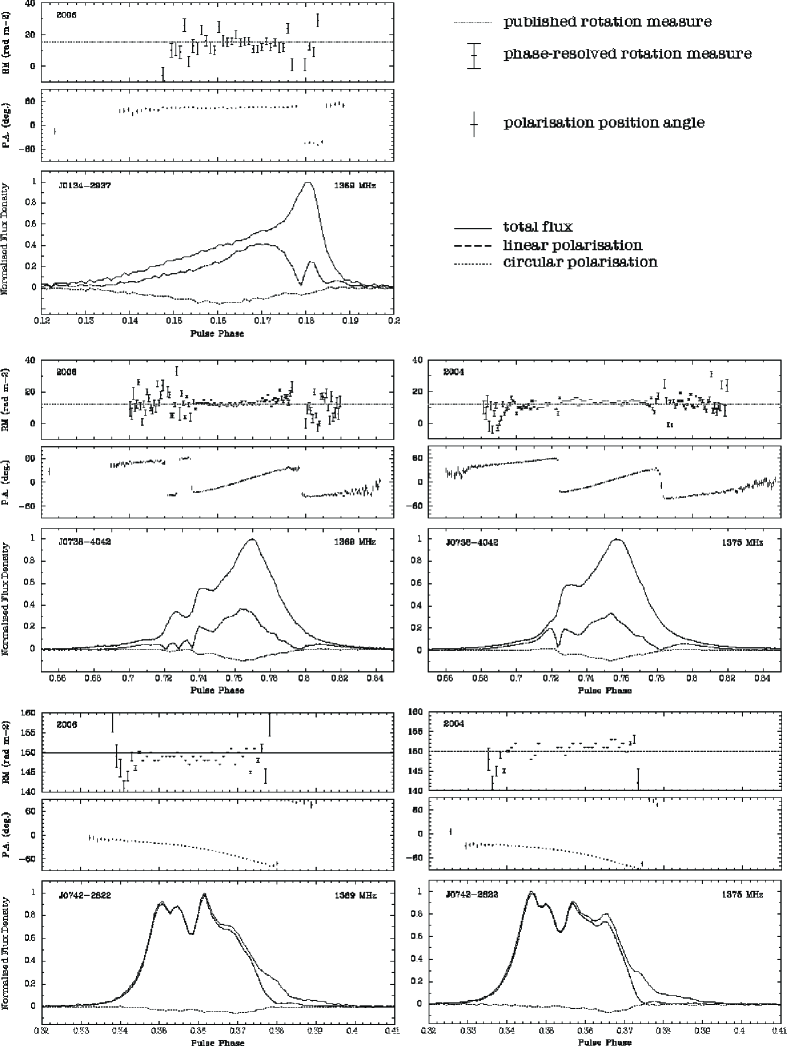
Figure 2: Profiles of the RM as a function of pulse longitude (top panels), for 10 pulsars, observed at 20 cm with the Parkes telescope, that exhibit small or no RM variations across their pulse profile. The respective year of observation is shown at the top-left corner of each pulsar’s RM profile. For two pulsars, namely PSR J0738$-$4042 and PSR J0742$-$2822, we had data from two observing sessions, in 2004 and 2006. See Fig. 1 for more details.

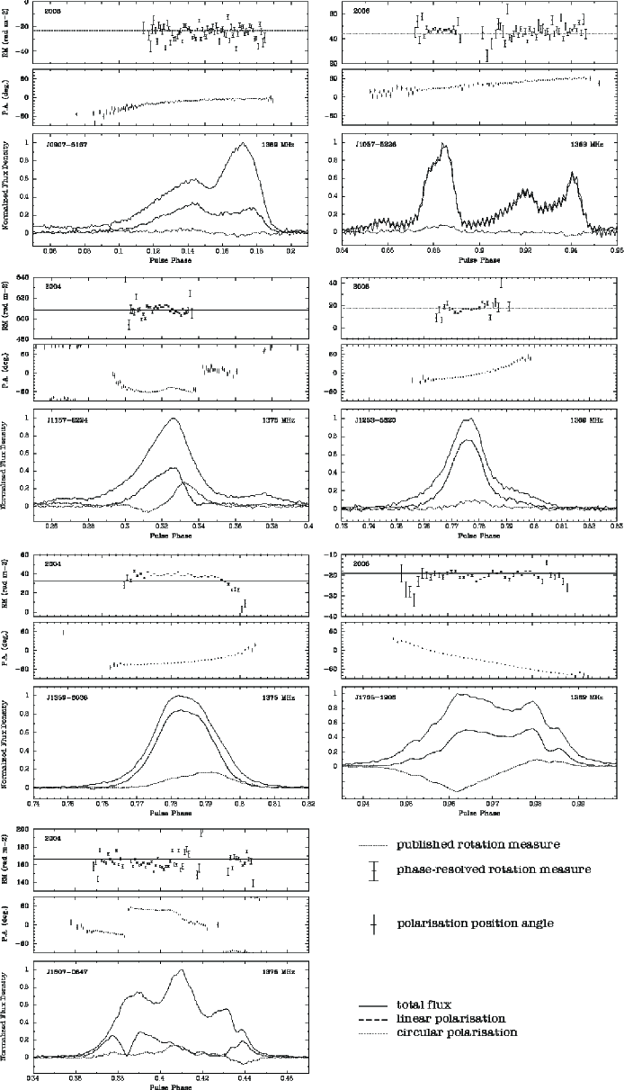
Figure 2: Continued

The resulting 19 RM profiles are shown in Fig. 1 and Fig. 2. 9 pulsars show large RM variation across the pulse and 10 pulsars show a rather constant RM profile. In these plots, the bottom panel shows the polarization profile, where solid lines denote total power; dashed lines, linear polarization; and dotted lines, circular polarization. The middle panels show the integrated PA profile and the top panels, the RM profile. In the interest of characterisation, we have included a number of properties of the pulsar emission and the ISM in the direction of the 19 pulsars, in Table 1.

3.1 Pulsars with large RM variation

PSR J0835$-$4510 (2004 & 2006 data). The Vela pulsar has a highly polarised, yet relatively simple pulse profile in both the 2004 and 2006 data. Both profiles appear scattered. The PA shows the characteristic swing which has been used as a strong argument for the rotating vector model (Radhakrishnan & Cooke 1969). The most striking profile of Vela is its RM profile, which shows a clear swing across the pulse that resembles a sideways ‘S’ (peak-to-peak variation $\approx 6$ rad m^-2). The shape of the RM profile persists through both 2004 and 2006 data sets, albeit the earlier of the two profiles displays a somewhat higher peak-to-peak variation of the RM ($\approx 13$ rad m^-2).

PSR J0942$-$5552 (2004 data). The pulse profile of this pulsar has 3 distinct components, with the peaks of linear polarization being slightly offset from the corresponding ones in the total power. The PA profile shows an orthogonal jump at the bridge emission between the leading and central components and at the exact phase where $L$ vanishes. The RM profile shows a steep decline of high-s/n points coincident with the leading end of the central component and an equally steep increase, coincident with the leading component; this behaviour occurs around the orthogonal PA jump. In both cases, the RM changes by at least 20 rad m^-2. At the central peak’s maximum the RM fluctuates within a few rad m^-2.

PSR J1056$-$6258 (2004 data). The total-power profile of this pulsar appears very slightly stretched toward later pulse phases. It has nearly zero circular polarization but $\approx 50$% linear. The PA profile sweeps smoothly across the pulse, without showing any breaks. The RM profile is roughly consistent with the published RM around the the flux maximum, but it drops suddenly near the pulse edges, giving it an overall shape of a swing across the entire pulse. [14] performed a comparison between the 20cm and 10cm profiles of this pulsar and concluded that the linear polarization, and hence the PA profile, must undergo significant frequency evolution. They supported their argument by deriving a pulse-averaged RM value for PSR B1056$-$6258 that was much closer to the published one (6 rad m^-2), whereas if no evolution was assumed that value was $-1$ rad m^-2. However, this pulsar shows a peak-to-peak RM variation across the pulse of almost 100 rad m^-2 — the highest in our sample — which dwarfs any possible RM error due to profile evolution.

PSR J1243$-$6423 (2004 data). The central pulse of this pulsar’s profile consists of two Gaussian components, whereas a third, much weaker component is present at the far leading edge of the profile. The circular polarization profile resembles an unsusual double swing, with its minimum value being roughly coincident with the maximum $L$. There is an orthogonal PA jump after the leading component. The PA profile corresponding to the central pulse components displays a full ‘S’-shaped swing, characterised by wiggles often seen in PA profiles. The RM profile of this pulsar is extremely complex: it shows a clear structure that departs from flatness, with a leading swing followed by a sharp peak and a steep decline of the RM. The peak-to-peak variation of the profile is $\approx 60$ rad m^-2. The maximum RM ($\approx 200$ rad m^-2) appears coincident with the inflexion point of the PA swing.

PSR J1326$-$5859 (2004 & 2006 data). This pulsar’s profile is the sum of at least two components: a weak leading one and a strong central one that leads into a trailing tail, perhaps indicative of a third, very weak component. The linear polarization of the central component is moderatly high, with more than 30% of its total flux being polarised, whereas the leading component is just over 20% polarised. Even more interesting is the evident swing of the circular polarization under the central component. Like in the case of PSR J1157$-$6224, this may well be hinting at emission from near the magnetic axis. In both epochs, the PA profile is broken by an orthogonal jump near the peak of the leading component, at the exact point where $L$ vanishes. At later phases, the PAs form an unusual swing interrupted mid-way by a bulge that is coincident with the maximum of the linear polarization. The RM profile clearly shows a smooth functional dependence on phase that deviates from flatness; like in the case of Vela, this dependence is exactly reproduced in both 2004 and 2006 data, which argues against this being an instrumental effect. The form of the RM function resembles a double swing with 2 local minima separated by a local maximum. The trailing of the two minima is exactly coincident with the peak in total power.

PSR J1453$-$6413 (2004 data). The pulse profile of this pulsar is a composition of a relatively weak leading component and a much stronger central one. However, in the linear-polarization profile these two components are of comparable intensity. The PA profile swings along the entire central component but is disrupted by an orthogonal jump that coincides with the merging point of the two components’ linear polarization, where $L=0$. The RMs across the pulse show a moderate amount of scattering that prevents us from being certain about the existence of a possible structure. On one hand, there is a clear break in the RMs due to the jump in the PAs. On the other hand, even away from the jump there seems to be a dip in the RMs that is coincident with the peak of the central component’s linear polarization.

PSR J1644$-$4559 (2004 data). The total power of this pulsar can be described by a single Gaussian with an extended, trailing scattering tail (see also analysis by Johnston 2004). A hint at a second, very weak component can be seen near the leading edge of the main pulse. The maximum of the linear polarization occurs at slightly earlier phase than that of the total-power maximum. In addition, this pulsar exhibits a swing in the circularly polarised profile. The PA profile shows a more complex picture, in comparison: it features two smooth bumps across the main pulse, which are only interrupted by an approximately orthogonal jump, coincident with the bridge emission between the main pulse and the weak leading component; it also shows the obvious signs of scattering on polarization shown in Li & Han (2001). The RM profile features a clear structure that comprises at least three local maxima and an equal number of local minima; none of these extremes is exactly coincident with either the total flux or the linearly polarised flux extremes. The fluctuation of the RM across the pulse appears mildly correlated to the PA profile.

PSR J1745$-$3040 (2004 data). There are three, distinct, highly polarised components in this pulsar’s profile. [10] performed multifrequency observations of this pulsar and noted the significant frequency evolution of its profile as well as the apparent increase of the linear polarization fraction with frequency. The PA profile resembles an upside-down $\upsilon$ across the trailing and central components, which is interrupted by an orthogonal jump occuring between the trailing components and the leading one. The RM profile shows a seemingly constant downwards slope for the most part of the two trailing components but kinks downwards at the leading edge of the central component. Above the leading component, the RMs are scattered, although an upwards slope can perhaps be inferred from the 6 data points coincident with this component.

PSR J2048$-$1616 (2006 data). Three Gaussian components can be discerned in the total profile of this pulsar. The linear polarization is strong in the leading and trailing of the three components but relatively weak in the central one. The PA profile resembles an ‘S’-shaped swing that rotates the PAs smoothly across the profile (see also Johnston et al. 2007; Johnston et al. 2008). The RM is rather constant across the leading component but dips by $\approx 8$ rad m^-2 at the central, least-polarised component. A sudden rise of the RMs is observed on the trailing edge of the trailing component, although the s/n of the linear polarization is already low in that phase region.

3.2 Pulsars with low RM variation

PSR J0134$-$2937 (2006 data). The PA profile of this pulsar is flat everywhere, apart from the phase region around the pulse maximum, where the profile is broken by an orthogonal jump. The jump is also coincident with the narrowest of the two distinct components present in the linearly polarised flux, the other being broad and coincident with the long leading tail of the total flux. The RM profile of this pulsar shares the same flatness, which seems to be disturbed by the presence of the orthogonal jump. However, the RM fluctuation occurs only over a few phase bins, and its magnitude is of the same order as at least three other instances away from the orthogonal jump.

PSR J0738$-$4042 (2004 & 2006 data). The polarization of this pulsar was shown at two frequencies (1.4 and 3 GHz) in Karastergiou & Johnston (2006). The position angle shows two orthogonal-mode jumps. The RM profile, although generally flat, is below the average RM value in the leading part of the profile; it then turns above the average RM value for the rest of the profile, after the first orthogonal jump. In the dual frequency data of Karastergiou & Johnston, the frequency evolution of the position-angle profile is in agreement with what is seen here: the first segment of the PA profile has a different frequency dependence to the rest of the profile.

PSR J0742$-$2822 (2004 & 2006 data). This pulsar comprises a complex, 7-component profile (see e.g. Kramer 1994; Karastergiou et al. 2005). Despite the complexity of the pulse itself, the PA and RM profiles display a relatively simple dependence on phase, with the former being a simple sweep across the profile and the latter being rather flat. It is perhaps noteworthy that a comparison between the profiles of 2004 and 2006 shows that the average RM in the earlier observations appears slightly higher than the published value, whereas the opposite is observed in 2006. The $\langle{\rm RM}\rangle$ difference between the two data sets is $\approx 5$ rad m^-2.

PSR J0907$-$5157 (2006 data). The total-power and linear-polarization profiles of this pulsar have two components. The PA profile is a smooth, continuous sweep, without any breaks, and one can notice that it slopes slightly upwards, toward the trailing edge of the pulse profile. The RM profile is flat and consistent within the errors with the published RM.

PSR J1057$-$5226 (2006 data). This young pulsar ($5.4\times 10^{5}$ y) is an interesting and a peculiar one, and one of a few that are visible at all wavelengths (see e.g. Vaughan & Large 1972; Cheng & Helfand 1983; Migniani et al. 1997; Fichtel et al. 1994). Even more interesting is its strong radio interpulse, which is separated from the main pulse by roughly 150^∘ and has the same energy as the main pulse over a wide range of radio frequencies (McCulloch et al. 1976; Weltevrede & Wright 2008 MNRAS submitted); it has been suggested that we observe emission from both magnetic poles (Lyne & Manchester 1988; Wang et al. 2006). Furthermore, the steepness of the PA swing for the main pulse and the interpulse differs significantly, which has given rise to the suggestion that the corresponding emission is generated at different heights in the magnetosphere (Wang et al. 2006). Due to the higher degree of linear polarization ($\sim 90\%$) and the modest s/n of the pulse in the 2006 data, we chose to study only the main pulse for RM variations. The PA profile of the main pulse is flat, with no breaks, and shows rotation of no more than 60^∘ across the entire pulse. The RM profile is also consistent with a constant RM.

PSR J1157$-$6224 (2004 data). This pulsar shows a simple total-power profile, with substantial amounts of linear ($>25$%) and circular polarization. The PA profile exhibits a smooth but complex swing, broken only by an orthogonal jump half-way along the trailing edge of the pulse. The RM profile also swings, although the edges are too noisy and the magnitude of the effect too small to draw a certain conclusion.

PSR J1253$-$5820 (2006 data). This pulsar’s pulse profile can be fitted with a single Gaussian component, and the same pulse shape is shared by the linearly polarised flux, which accounts for a large fraction of the total observable emission. The PA shows a smooth variation throughout. The RM profile shows little deviation from flatness, mainly at the leading edge.

PSR J1359$-$6038 (2004 data). This pulsar’s profile is $>70$% linearly polarised and $\approx 15$% circularly polarised. The PA profile is rather flat across the pulse. The RM profile is consistent with a constant value for the most part of the profile, diverging slightly at the tail end, similarly to PSR J1056$-$6258. However, at that point the s/n is greatly reduced so solid conclusions cannot be extracted.

PSR J1705$-$1906 (2006 data). This is another highly polarised pulsar with a main pulse composed of multiple components: despite having been classified as a three-component pulse, at least five components can be discerned in both the total power and the linear polarization profiles in our data (Rankin 1990; Gould & Lyne 1998). In addition, a much simpler, single-peaked interpulse is also present in this pulsar’s profile, which is separated by roughly $180^{\circ}$ from the main pulse. At 20cm, the interpulse is almost 100% linearly polarised, which has also been noted in previous work (see e.g. Karastergiou & Johnston 2004). In this work, we chose to examine only the main pulse for RM variations, due to its larger width and higher s/n. The PA profile is a gradual sweep across the entire main pulse. The RM profile appears flat, on average, although a coherent jitter over a-few-bin scale is evident. The only possible departure from flatness appears to coincide with the leading outrider.

PSR J1807$-$0847 (2004 data). Another case of a multi-component, total-power profile, with low linear polarization and with a central component surrounded by at least three outriders. The PA profile is broken twice by orthogonal jumps, which coincide with the minima of the linear polarization; this has also been noted in a separate analysis by [14]. The RM profile is quite noisy, owing to the low linear polarization, but flat, on average, across the entire pulse.

3.3 Fit Accuracy Across the Band

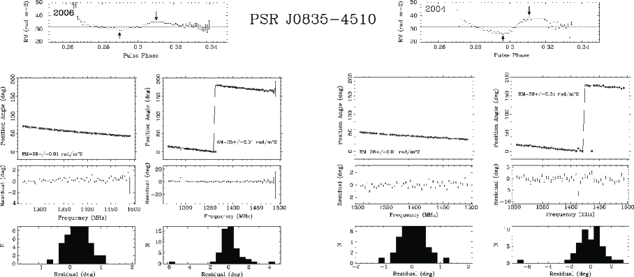
Figure 3: RM fits to the PAs corresponding to the maximum- and minimum-RM values in the central part of Vela pulsar’s RM profile. The set of plots to the left of the pulsar’s J2000 name (J0835$-$4510) correspond to the 2006 data; the ones to right of the legend correspond to data collected in 2004. The top plots in each set show the RM variation across the pulse; below them, we show the RM fits corresponding to the minimum (left) and maximum RM (right) in the RM profile. The minimum- and maximum-RM values selected for the fits are indicated with black arrows in the respective RM profiles. Below each fit we show the fit residuals in degrees, and at the very bottom the distribution of those residuals is shown.

In order to check for the presence of any frequency-dependent, systematic effect that could cause a change of the PA across the frequency band that is different to the $\lambda^{2}$ law of Faraday rotation, we examined in more detail the fits that produced the calculated RMs for Vela, J1243$-$6423 and J1326$-$5859. Fig. 3, 4 and 5 show the RM fits for the minimum- and maximum-RM bins (denoted by arrows) that reside near the central part of the profile of the three aforementioned pulsars. It is important to note that the associated errors on the fitted RMs, being only statistical, would be underestimated if there was an additional, systematic, non-Faraday component that affects the PAs. In order to reveal the presence and magnitude of a possible systematic discrepancy between the fitted function and the data, for each fit we also plotted the fit residuals and their distribution (shown below the fit plots, in Fig. 3, 4 and 5). The quality of the data and the goodness of the fit are evident in these figures. Upon closer inspection, however, the residual PAs of all three pulsars, but mostly J1243$-$6423 and J1326$-$5859, show evidence of some weak, sinusoidal fluctuations around the mean. It is difficult to attribute some significance to this, especially given the Gaussian-like distributions of the residuals. The conclusion therefore is that, if there is indeed a physical mechanism that affects the PA rotation, apart from the interstellar Faraday effect, we are unable to distinguish it from the dominant $1/f^{2}$ law.

3.4 DM errors

We also investigated the possibility that the RM variations observed are caused by erroneous estimation of the DM, with, say, a $\Delta{\rm DM}$ offset from the true value. Such an offset is translated into a dispersive delay between the pulse arrival time at a reference frequency $f_{0}$ (usually the centre frequency of the band) and that at frequency $f=f_{0}+\Delta f$, where $\mid\Delta f\mid\ll f_{0}$. In that case, the delay in ms is given by

$$\Delta t=8.3\times 10^{6}{\rm ms}\ \ \frac{\Delta f}{f_{0}^{3}}\Delta{\rm DM}$$ (3)

which also corresponds to a phase offset in the pulse window, $\Delta\phi=\Delta t/P$, with $P$ the pulsar period.

If this phase offset is not accounted for, the calculation of the PA in each frequency channel will correspond to a pulse longitude that is shifted with respect to that at the reference frequency; this may introduce a frequency-dependent shift in the PA of any given phase bin. In order to eliminate this as the cause of the observed RM variations, we de-dispersed our data using the published DM value, as well as two other values that were $5\sigma$ away, either side of the published one, and generated again the RM profile in each case. The published DMs for our pulsars are shown in Table 1. By checking the resulting RM profiles for all pulsars, we concluded that there is no way of recovering a flat RM curve for any reasonable departure from the published DM. We therefore rule out DM errors as a possible cause of RM variation.

4 Discussion

Our analysis reveals that the RM profiles of pulsars with large RM variations are diverse: they can be as simple as the ‘S’-shaped profiles of Vela and PSR J1056$-$6258 or as complex as those of PSR J1243$-$6423 and PSR J1644$-$4559. The peak-to-peak variation of those pulsars’ RMs across their profiles was found to be as little as a few rad m^-2 (e.g. Vela in 2006) but also as large as 100 rad m^-2, for PSR J1056$-$6258. Despite the hints of correlation between individual features in the flux and PA profiles and those in the RM profiles (see e.g. PSR J1326$-$5859), in most cases these correlations seem coincidental. However, a general observation is that the greatest RM fluctuations across the pulse profile seem coincident with the steepest gradients of the PA profile, whereas pulsars with flat PA profiles show little or none at all RM variation. Good examples that support this argument are PSR J1243$-$6423 and PSR J2048$-$1616, whose RM departure from the mean is maximised around the inflexion point of the PA swing; in contrast, PSR J0907$-$5157 and PSR J1057$-$5226, having flat PA profiles, show insignificant RM variations.

The subset of pulsars with low RM variations adheres to the theoretical predictions. More than half of those pulsars have phase-resolved RMs that are scattered around their respective published RM value, thus showing convincingly longitude-independent RM values across the pulse. However, there are cases like those of PSR J1157$-$6224, PSR J1253$-$5820, PSR J1359$-$6038 and PSR J1705$-$1906, where the RM scatter across the pulse is clearly not Gaussian: these profiles show a clear structure but with a small RMS spread. An interesting case is that of PSR J0742$-$2822, where although no significant RM variations exist across the profile, the longitude-averaged RM across the pulse is higher in 2004 data than in 2006. Nevertheless, one has to be careful when drawing the above conclusions; the main statement is that any RM variations with pulse phase are smaller than the statistical error of the measurement.

We have demonstrated that the RM variations observed are not due to measurement errors, and that the PA rotation in all cases follows the $\lambda^{2}$ law of Faraday Rotation. In the following we consider three possible explanations: (a) Faraday Rotation within the pulsar magnetosphere, (b) the superposition and frequency dependence of quasi-orthogonal polarization modes, and (c) interstellar scattering and its effects on the polarization.

4.1 Magnetoshperic Faraday Rotation

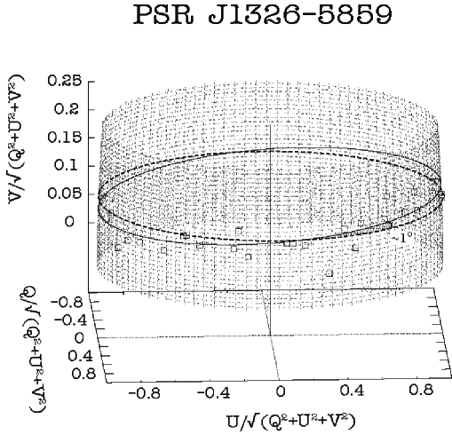
Figure 6: The rotation of the Poincaré vector, $\hat{\boldsymbol{P}}$, as a function of frequency, across the frequency band, for PSR J1326$-$5859. The 3D representation of the rotation is zoomed into the latitude range which contains the data. The data points were best fitted with a circle of inclination $1.3^{\circ}\pm 0.6^{\circ}$ (solid black line), whereas a flat circle of zero inclination (dashed black line) gave a worse fit.

Faraday Rotation through the ionised ISM has the effect of rotating the PA with frequency. Our data, however, comprise of full sets of the four Stokes parameters, $I$, $Q$, $U$ and $V$, so we can observe the frequency dependence of the entire polarization vector ($\hat{\boldsymbol{P}}=(Q\hat{\boldsymbol{i}}+U\hat{\boldsymbol{j}}+V\hat{\boldsymbol{k}})/\sqrt{Q^{2}+U^{2}+V^{2}}$) as a function of frequency, for specific high-s/n phase bins. An example for one phase bin of PSR J1326$-$5859 is shown in Fig. 6, where the tip of the Poincaré vector is plotted across 32 frequency channels. This plot demonstrates that, together with the pronounced effect of PA rotation (around the vertical axis), a small and rather systematic change in the fraction of circular polarization can be seen. We obtained similar plots for four additional pulsars in our sample that displayed large RM variations: namely Vela, PSR J1243$-$6423, PSR J1644$-$4559 and PSR J2048$-$1616. In nearly all cases, we found that the trace of $\hat{\boldsymbol{P}}$ on the Poincaré sphere does not strictly follow paths of constant latitude, as in Fig. 6.

The wave modes in the cold and ionised ISM are purely circularly polarised. Therefore, the phase offset introduced by propagation through this medium results in the well-documented changes of the PA. On the contrary, in a medium of highly relativistic charged particles, the natural modes are close to linearly polarised (Sazonov 1969; Melrose 1997a). As a consequence, different phase offsets between the modes will result in a conversion between linear and circular polarization. In a pulsar’s magnetosphere, the observed degrees of circular polarization indicate that the natural wave modes are elliptically polarised, which suggests that propagation through this medium will generate some frequency-dependent conversion between linear and circular polarization. An extensive discussion on this can be found in [16].

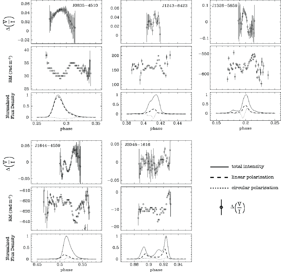
Figure 7: Top panels: the change in the fraction of circularly polarised intensity across the band as a function of pulse longitude, for Vela, PSR J1243$-$6423, PSR J1326$-$5859, PSR J1644$-$4559 and PSR J2048$-$1616. For comparison, we have included, in the middle and bottom panels, the RM and polarization profiles of each pulsar.

If such a generalised Faraday Rotation is taking place within the pulsar magnetosphere and giving rise to RM variations as well as changing the degree of circular polarization in the observed frequency band, we expect the greatest change in $V$ to coincide with the greatest variations in RM. In order to test this, we first calculated the fraction of circularly polarised intensity, $V/I$, for each frequency channel across the band. The division by $I$ removes any fluctuations of $V$ caused by scintillation through the interstellar medium, whereas any change in $V$ that originates in the magnetoshpere should remain unaffected. Subsequently, we fitted a linear function, $V/I\propto f$, to the data and calculated the change in $V/I$ across the band, based on that function. This was done to get a good estimate of the total effect while minimizing the influence of instrumental noise. We found linear fits to describe the data sufficiently well. The resulting profiles of $\Delta(V/I)$ as a function of longitude, for Vela, PSR J1243$-$6423, PSR J1326$-$5859, PSR J1644$-$4559 and PSR J2048$-$1616 are shown in Fig. 7. A side-by-side comparison of the RM and $\Delta(V/I)$ profiles, shown in Fig. 7, makes clear that none of the pairs of profiles seems correlated.

There is certainly little evidence that the maximum RM deviation from the mean and the maximum change in circular polarization across the band occur at the same pulse phase. Therefore, to first order, the assumption that the observed RM variations are caused by magnetospheric Faraday rotation is deemed unlikely.

4.2 Quasi-orthogonal Emission Modes

Another factor that could potentially affect the measured RM is the incoherent superposition of quasi-orthogonal modes of polarization (see e.g. Ramachandran et al. 2004). The superposition of strictly orthogonal modes results in an observed PA of the strongest of the two modes, regardless of the ratio of the intensity of the modes (e.g. Backer et al 1976; Cordes et al. 1978). The reason is that orthogonal modes are represented by anti-parallel vectors on the Poincare sphere; regardless of their relative lengths, the addition is always pointing in the direction of either of the two modes. This is not the case for non-orthogonal modes: in this case, the sum of the mode vectors points at an angle that depends on the degree of non-orthogonality and the relative intensity of the modes. As a consequence, if the ratio of the mode intensities changes as a function of frequency, the observed PA will also rotate. The question is under what conditions this could resemble Faraday Rotation.

In the pulsars where significant RM variations are seen, the variations often exceed 20 rad m^-2 across the pulse profile. At the frequency and bandwidth of these observations, this corresponds to a variation in PA by $\sim 18.5^{\circ}$. Therefore, in order for quasi-orthogonal polarization modes to present a possible explanation for the observed RM variations, they should be capable of inducing such a PA rotation.

From polarization studies of 18 pulsars in the European Pulsar Network (EPN) archive, [29] conclude that the ratio of the average intensity of the orthogonal modes for those pulsars follows a power law with spectral index that does not typically exceed $\gamma\sim-0.5$. Assuming linear modes ($L_{1}$ and $L_{2}$; the degree of circular polarization is generally very low), then at a reference frequency $f_{0}$ the mode intensity ratio is $R_{0}=L_{1}/L_{2}$, and the form of this power law is

$$R=R_{0}\left(\frac{f}{f_{0}}\right)^{-0.5}$$ (4)

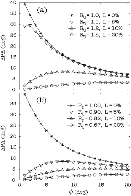
Figure 8: The total PA difference between 1300 and 1556 MHz due to the frequency evolution of the relative strength of quasi-orthogonal modes, as a function of the angle of departure from orthogonality, $\phi$, and for (a) increasing and (b) decreasing values of the initial relative intensity of the modes $R_{0}$, as indicated.

For given values of $R_{0}$, we can compute $R$ across the frequency band we are interested in: in this case, between 1300 and 1556 MHz. We have numerically computed the total rotation of the PA across the band (hereafter $\Delta$PA), for different values of $R_{0}$ and different angles of non-orthogonality, $\phi$. The latter angle is defined on the Poincarè sphere as the supplementary to the angle between the two modes. Figure 8 shows $\Delta$PA versus $\phi$, for various values of $R_{0}$, which equate to certain degrees of linear polarization. The plot on the left shows examples where $R_{0}\geq 1$ as opposed to $R_{0}\leq 1$ for the plot on the right. Both plots show a set of lines corresponding to the same degrees of polarization , $L$%, which is approximately $\mid L_{1}-L_{2}\mid/I$. Two things are immediately evident: first, the greatest rotation of PA happens for small values of $\phi$; second, and most important, the only possibility that $\Delta$PA$>15^{\circ}$ occurs when the fractional polarization remains under 10% and only in the specific case where $R_{0}>1$, i.e. the case where the mode with the steepest spectral index is brightest at the lowest frequency $f_{0}$. In our data, there are clear examples of high $\Delta$RM and high $L$%, the most prominent being Vela and J1326$-$5759. It is therefore unlikely that non-orthogonal polarization modes provide a general explanation for the RM variations in the data.

4.3 Scattering

As was mentioned earlier in this paper, some of the pulsars we studied show signs of interstellar scattering in their flux profiles: vivid examples are PSR J1056$-$6258, justified by its high DM of 320.3 pc cm^-3, and PSR J1644$-$4559, with a DM of 478.8 pc cm^-3 — the highest in our sample. We checked for a possible correlation between the amount of interstellar scattering and the magnitude of the observed RM variations. The effect of interstellar scattering is usually quantified by the scattering timescale, $\tau_{\rm sc}$. Assuming a Kolmogorov spectrum for the density fluctuations along the sightline to the pulsar, $\tau_{\rm sc}$ has a roughly quadratic relation to DM for low-DM pulsars (i.e. $\tau_{\rm sc}\propto{\rm DM}^{2}$) but can be much steeper for high-DM pulsars: i.e. $\tau_{\rm sc}\propto{\rm DM}^{4}$ (e.g. Sutton 1971; Ricket 1977). More recently, based on a global fit to 98 scattering times of high-DM pulsars, [2] showed that a parabolic curve of the form

$$\log\tau_{\rm sc}=-6.46+0.154\log{\rm DM}+1.07(\log{\rm DM})^{2}-3.86\log{f_{0}}$$ (5)

where $f_{0}$ is the observing frequency, is a reasonable description of the trend of $\tau_{\rm sc}$ as a function of DM. Hence, as long as we are refering to the same observing frequency, and since there are only a few available measurements of $\tau_{\rm sc}$ for our pulsar sample (see Table 1), the DM is a convenient alternative to the amount of scattering a pulsar’s emission is subject to.

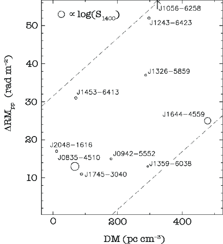
Figure 9: Scatter plot of the maximum, peak-to-peak RM difference ($\Delta{\rm RM}_{\rm pp}$) as a function of the pulsar DM, measured across the profiles of the 9 pulsars that show large RM variations and PSR J1359$-6038$, for which a lesser degree of RM variation is visible. The arrow at the top of the frame indicates that the $\Delta{\rm RM}_{\rm pp}$ value measured for PSR J1056$-$6258 ($\sim 100$ rad m^-2) is off the plot’s scale. The symbol size in this plot is proportional to the logarithm of the average flux at 1.4 GHz, $S_{1400}$.

We have quantified the magnitude of the RM variations for those pulsars whose RM profiles show signs of a longitude-dependent structure, in terms of the peak-to-peak distance of their RM profile, $\Delta{\rm RM}_{\rm pp}$. Fig. 9 shows a scatter plot of $\Delta{\rm RM}_{\rm pp}$ against DM for 9 pulsars. Although there is perhaps no clear correlation, it is striking that the pulsars that typify high RM variations are also high-DM pulsars. This includes the most prominent examples of RM variation with pulse phase, such as PSR J1243$-$6423, PSR J1326$-$5859 and PSR J1644$-$4559. In a recent paper, [12] showed that small amounts of scattering and orthogonal polarization modes of emission in the pulsar magnetosphere can result in a frequency dependent PA that can be falsely attributed to Faraday Rotation. This explanation is extremely simple and may well be the key to understanding the high-DM examples. It is also strengthened by the observation that most of the low-DM pulsars show relatively smooth PA profiles, devoid of the bumps and wiggles seen in the higher DM profiles. The overall correlation in Fig. 9 is perhaps reduced by the fact that RM measurements can only be made for pulse phases with significant linear polarization.

5 Conclusions

We have shown phase-resolved RM profiles for 19 pulsars, 9 of which show substantial RM variations across the pulse profile. These variations appear in most cases to show coherent rather than noisy behaviour. The high s/n of our data and our robust fitting technique have shown that whatever the cause of the PA rotation with frequency, it is inseparable from the $1/f^{2}$ law of interstellar Faraday Rotation within our observed band.

We have considered a number of possibilities that may result in the observed phenomena. For example, we have ruled out the possibility that de-dispersion with a slightly erroneous DM may be responsible for the data here. We have discussed the possibility that the RM variations are of magnetospheric origin. Two cases were examined, that of generalised Faraday Rotation due to the relativistic plasma in the pulsar magnetospheres, and the existence and superposition of quasi-orthogonal modes of polarization.

In the case of generalised Faraday Rotation, we examined whether pulse phases with the highest rotation of the PA also showed the highest change of the fractional circular polarization. Our first-order investigation turned out negative results, although it is true that the theory for generalised Faraday Rotation is not complete and does not provide us with good handles on the rate at which polarization rotations occur with frequency.

As concerns quasi-orthogonal modes, we find that it is impossible to obtain a large rotation of the PA within our observing frequency band and observe large degrees of linear polarization at the same time. Our analysis indicates that there are specific cases of the data that can be explained by this process, but it certainly does not form a general framework for explaining RM variations across the pulse.

Finally, this work supports the ideas presented in [12], that interstellar scattering can distort the polarization in a frequency-dependent way. This may resemble Faraday Rotation and will generally be pulse-phase dependent. It is important to emphasise that the possibility of magnetospheric Faraday Rotation is not totally eliminated by this work; we merely conclude that it is an unlikely explanation for RM variations of the observed magnitude.

There is a possibility that both the magnetospheric mechanisms and interstellar scattering are responsible for the observed RM variations, along with other possibe mechanisms which we have not considered. Whichever the explanation, certain care must be taken during RM-determination experiments from pulsars to correctly identify the amount of PA rotation that is due to the iono-magnetised interstellar medium. Especially for the studies of the planar component of the Galactic magnetic field, where pulsars with high DMs and RMs are used, the identification of the ISM-induced Faraday rotation and the correct calculation of the associated RM plays an important role in our efforts to model the interstellar magnetic fields. Hence, in light of the RM profiles presented herein, pulsar-RM determination from specific, high-s/n pulse bins can lead to considerable errors.

Table 1: Tabulated properties of the 19 pulsars we analysed in this work. Columns 7 and 8 show the pulse-averaged fraction of the linearly and circularly polarised intensity, respectively. The last column shows the magnitude of the interstellar pulse broadening as a percentage of the pulse’s FWHM; this is only known for 6 pulsars in our sample.

PSR	$P$	DM	$\sigma_{\rm DM}$	RMpub	$\sigma_{\rm RM}$	$L/I$	$V/I$	$\Delta{\rm RM}_{\rm pp}$	$S_{1400}$	$\tau_{\rm sc}/{\rm W}_{50}$
	[s]	[pc cm-3]	[pc cm-3]	[rad m-2]	[rad m-2]	[%]	[%]	[rad m-2]	[mJy]	[%]
J0134$-$2937	0.1369	21.806	0.006	15	3	41	19	0	2.4	–
J0738$-$4042	0.3749	160.8	0.7	12.1	0.6	29	6	0	80	–
J0742$-$2822	0.1667	73.782	0.002	148.5	0.6	88	3	0	15	0.14
J0835$-$4510	0.0893	67.99	0.01	30.4	0.6	88	7	13	1100	3
J0907$-$5157	0.2535	103.72	–	$-$23.3	1	32	4	0	9.3	–
J0942$-$5552	0.6643	180.2	0.5	$-$61.9	0.2	33	8	15	10	–
J1056$-$6258	0.4224	320.3	0.6	4	2	50	2	100	21	–
J1057$-$5226	0.1971	30.1	0.5	44	2	86	4	0	–	–
J1157$-$6224	0.4005	325.2	0.5	508.2	0.5	26	12	0	5.9	–
J1243$-$6423	0.3884	297.25	0.08	157.8	0.4	20	13	52	13	–
J1253$-$5820	0.2554	100.584	0.004	31	5	57	6	0	3.5	–
J1326$-$5859	0.4779	287.30	0.15	$-$579.6	0.9	32	17	37	9.9	38
J1359$-$6038	0.1275	293.71	0.14	33	5	73	15	13	7.6	–
J1453$-$6413	0.1794	71.07	0.02	$-$18.6	0.2	24	6	31	14	–
J1644$-$4559	0.4550	478.8	0.8	$-$617	1	17	3	25	310	136
J1705$-$1906	0.2989	22.907	0.003	$-$9	4	72	27	0	8	–
J1745$-$3040	0.3674	88.373	0.004	$-$19.2	1	49	5	11	13	–
J1807$-$0847	0.1637	112.3802	0.0011	166	9	23	9	0	15	0.03
J2048$-$1616	1.9615	11.456	0.005	$-$10.2	0.8	37	4	17	13	$10^{-6}$

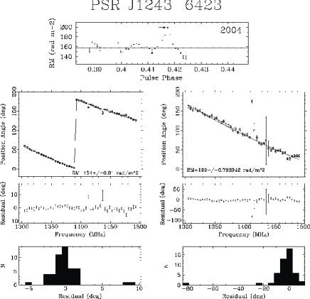
Figure 4: RM fits for J1243$-$6423. See Fig. 3 for details.

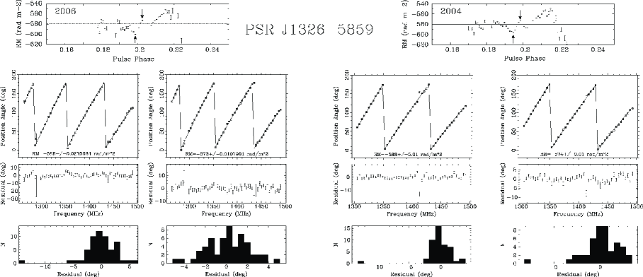
Figure 5: RM fits for J1326$-$5859. See Fig. 3 for details.

References

- [1] Backer D. C., Rankin J. M., Campbell D. B., 1976, Nature, 263, 202
- [2] Bhat N. D. R., Cordes J. M., Camilo F., Nice D. J., Lorimer D. R., 2004, ApJ, 605, 759
- [3] Cheng A. F., Helfand D. J., 1983, ApJ, 271, 271
- [4] Cordes J. M., Rankin J. M., Backer D. C., 1978, ApJ, 223, 961
- [5] Fichtel C. E., Bertsch D. L., Chaing J., Dingus B. L., Esposito J. A., Fierro J. M., Hartman R. C., Hunter S. D., Kanbach G., Kniffen D. A., 1994, ApJS, 94, 551
- [6] Gould D. M., Lyne A. G., 1998, MNRAS, 301, 235
- [7] Hotan A. W., van Straten W., Manchester R. N., 2004, PASA, 21, 302
- [8] Johnston S., 2002, Pub. of the ASA, 19, 277
- [9] Johnston S., 2004, MNRAS, 348, 1229
- [10] Johnston S., Karastergiou A., Mitra D., Gupta Y., 2008, MNRAS, 388, 261
- [11] Johnston S., Kramer M., Karastergiou A., Hobbs G., Ord S., Wallman J., 2007, MNRAS, 381, 1625
- [12] Karastergiou A., 2009, MNRAS, 392, L60
- [13] Karastergiou A., Johnston S., 2004, MNRAS, 352, 689
- [14] Karastergiou A., Johnston S., 2006, MNRAS, 365, 353
- [15] Karastergiou A., Johnston S., Manchester R. N., 2005, MNRAS, 359, 481
- [16] Kennett M., Melrose D., 1998, PASA, 15, 211
- [17] Kramer M., 1994, A&AS, 107, 527
- [18] Li X. H., Han J. L., 2003, A&A, 410, 253
- [19] Lyne A. G., Manchester R. N., 1988, MNRAS, 234, 477
- [20] McCulloch P. M., Hamilton P. A., Ables J. G., Komesaroff M. M., 1976, MNRAS, 175, 71P
- [21] Melatos A., 1997, MNRAS, 288, 1049
- [22] Mignani R., Caraveo P. A., Bignami G. F., 1997, ApJ, 474, L51
- [23] Noutsos A., Johnston S., Kramer M., Karastergiou A., 2008, MNRAS, 386, 1881
- [24] Radhakrishnan V., Cooke D. J., 1969, Astrophys. Lett., 3, 225
- [25] Ramachandran R., Backer D. C., Rankin J. M., M. W. J., E. D. K., 2004, ApJ, 606, 1167
- [26] Rankin J. M., 1990, ApJ, 352, 247
- [27] Rickett B. J., 1977, Ann. Rev. Astr. Ap., 15, 479
- [28] Sazonov V. N., 1969, Soviet Journal of Experimental and Theoretical Physics, 29, 578
- [29] Smits J. M., Stappers B. W., Edwards R. T., Kuijpers J., Ramachandran R., 2006, A&A, 448, 1139
- [30] Sutton J. M., 1971, MNRAS, 155, 51
- [31] Vaughan A. E., Large M. I., 1972, MNRAS, 156, 27P
- [32] Wang H. G., Qiao G. J., Xu R. X., Liu Y., 2006, MNRAS, 366, 945