Asymptotically vanishing ${\cal PT}-$symmetric potentials and negative-mass Schrödinger equations

Miloslav Znojil, Petr Siegl

Nuclear Physics Institute of Academy of Sciences of the Czech Republic, 250 68 Řež, Czech Republic,

and

Géza Lévai

Institute of Nuclear Research of the Hungarian Academy of Sciences,

PO Box 51, H-4001 Debrecen, Hungary

Abstract

In paper I [M. Znojil and G. Lévai, Phys. Lett. A 271 (2000) 327] we introduced the Coulomb - Kratzer bound-state problem in its cryptohermitian, ${\cal PT}-$symmetric version. An instability of the original model is revealed here. A necessary stabilization is achieved, for almost all couplings, by an unusual, negative choice of the bare mass in Schrödiner equation.

1 Introduction

Intuitively one feels that for Schrödinger equations

$$\frac{\ \hbar^{2}}{2m}\,\left[-\frac{d^{2}}{d{x}^{2}}+\frac{L(L+1)}{{x}^{2}}\right]\,\Psi({x})+V(x)\,\Psi({x})=E\,\Psi({x})\,$$ (1)

there should exist a close connection between the reality of potential $V(x)$ and the reality of the corresponding energies $E$. Unfortunately, such a type of intuition proves deceptive. Recent studies (e.g., [1] or [2]) showed that many manifestly non-Hermitian potentials, e.g.,

$$V^{(BB)}(x)=x^{2}\,({\rm i}x)^{4\delta}\,,\ \ \ \ \ \ \delta\geq 0\,$$ (2)

still lead to a full reality of the spectrum. The key to such an unexpected phenomenon can be seen in the Bender’s and Boettcher’s [1] fortunate choice of a complex integration contour $x=x^{(BB)}(s)$ in eq. (1). Its asymptotes

$$x^{(BB)}(s)\ \approx\ \left\{\begin{array}[]{ll}s\,e^{{\rm i}\varphi}\,,&s\gg 1\,,\\ s\,e^{-{\rm i}\varphi}\,,&s\ll-1\end{array}\right.$$ (3)

were restricted to the $\delta-$dependent interval of angles,

$$\varphi+\frac{\pi}{2}\in\left(\frac{\pi}{4+4\delta},\frac{3\pi}{4+4\delta}\right)\,.$$ (4)

The curve itself was required not to cross the singularity of $V^{(BB)}(x)$ in the origin, ${\rm i}x^{(BB)}(0)>0$. In this setting one can impose the standard Dirichlet boundary conditions at the ends of the left-right-symmetric curve of complex coordinates, $\Psi({x^{(BB)}(\pm\infty)})=0$, with the computationally preferred slope lying precisely in the center of the interval,

$$\varphi^{(BB)}=\frac{\pi}{2+2\delta}-\frac{\pi}{2}\,.$$ (5)

In ref. [1] it has been emphasized that potentials (2) as well as paths of $x$ and angles (5) were chosen as symmetric with respect to the combination of the parity-reversal symmetry mediated by the operator ${\cal P}$ with the time-reversal symmetry represented by operator ${\cal T}$ (cf. also ref. [3] in this respect). In ref. [4] it has been added that for the other eligible domains of angles, say, for

$$\varphi+\frac{\pi}{2}\in\left(\frac{3\pi}{4+4\delta},\frac{5\pi}{4+4\delta}\right)\,$$ (6)

the reality of the spectrum breaks down at some non-vanishing exponents $\delta<\delta_{0}$. In this sense the specific ${\cal PT}-$symmetric choice of (2) – (4) giving $\delta_{0}=0$ may be considered optimal.

The discussions in refs. [1, 4] did not involve the negative exponents $\delta$ and, in particular, the short-range models where $V(\infty)=0$. The gap has partially been filled by ref. [5] where we studied eq. (1) with one of the simplest possible asymptotically vanishing ${\cal PT}-$symmetric potentials of the Coulomb-Kratzer two-parametric form,

$$V(x)=V^{(CK)}(x)=\frac{{\rm i}Z}{x}+\frac{F}{x^{2}}\,.$$ (7)

This model admits $\varphi\in\left(0,\pi\right)$ (cf. eq. (4) with $2\delta=-1$). From eq. (5) giving $\varphi^{(BB)}=\pi/2$ one arrives at the U-shaped complex-coordinate contours $x^{(BB)}(s)$ as sampled in Figure 1 where the cut is assumed from $x=0$ upwards. Marginally let us emphasize that our Schrödinger eq. (1) in the most common physical setting using an integer angular momentum $\ell=0,1,\ldots$ should in fact be considered with the “centrifugal-like” term of a non-integer strength $L(L+1)=\ell(\ell+1)+F$ in general.

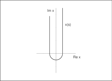
Figure 1: The optimal, U-shaped contour of the complexified coordinates $x^{(BB)}(s)$ for the Coulomb-Kratzer ${\cal PT}-$symmetric potential (7).

At the time of the publication of ref. [5] (to be cited as paper I from now on) the physical meaning of the similar models remained still rather obscure. Many authors studied and interpreted them as mere effective non-Hermitian simulations of spectra, not allowing any immediate physical interpretation of the related wave functions $\Psi(x)\in I\!\!L_{2}(I\!\!R)$. Although we also accepted the same philosophy in paper I, we were aware of the fact that such an attitude significantly weakened the impact and practical applicability of similar studies.

Fortunately, the subsequent development of the subject clarified that the potentials as exemplified by eq. (7) can be interpreted as fully compatible with the standard postulates and probabilistic interpretation of Quantum Mechanics. One of the most straightforward mathematical keys to the resolution of such an apparent puzzle can be seen in the existence of a suitable non-unitary invertible map $\Omega$ between some manifestly non-Hermitian Hamiltonians $H\neq H^{\dagger}$ and their manifestly Hermitian partners $\mathfrak{h}=\Omega\,H\,\Omega^{-1}$ (cf., e.g., ref. [6] for a compact explanation of this mathematical idea).

From the point of view of physics, the historical origin of the idea of relevance of isospectrality between $\mathfrak{h}$ and $H$ can be traced back to the study of models of atomic nuclei [7]. There an explicit example of operator $\Omega\neq(\Omega^{\dagger})^{-1}$ has been provided by the generalized Dyson mappings [8]. Our recent return to these physical studies in our mathematical review [6] showed that for the ${\cal PT}-$symmetric models all the probabilistic physical postulates of quantum theory remain valid.

Among immediate and most recent phenomenological applications of non-Hermitian, ${\cal PT}-$symmetric operators $H\neq H^{\dagger}$ with real spectra let us mention here just the preprint  [9] dealing with a ${\cal PT}-$symmetric version of a flat Friedmann model in quantum cosmology. In such a broader physical context we feel particularly inspired here by one of technical questions discussed in this paper and concerning the possible instabilities of generic ${\cal PT}-$symmetric systems. In this sense we also returned to our older results of paper I which will be re-evaluated, corrected and re-interpreted in what follows.

2 Free motion along asymptotes

In the majority of presentations of Schrödinger eq. (1) in textbooks one works with the real $x$ specifying the position of a particle or quasiparticle which carries a constant mass $m=m_{0}>0$. The influence of external forces is modeled solely by a potential $V(x)$. During the last few years a manifest coordinate-dependence of the mass term has been allowed as well [10]. The choice of $m=m(x)$ opened new perspectives in an optimal description of the effects of medium.

This idea could easily be transferred to the present class of models where $x=x(s)$ is complex and where the effect of the potential becomes negligible in the asymptotic domain of $|s|\gg 1$. In such a setting the mass can be perceived as a potentially position-dependent complex quantity, $m=m[x(s)]\in\,l\!\!\!C$.

At the large $|s|$ our Hamiltonians get approximated by the kinetic-energy operator $T$ which, by itself, gets complexified in the light of eq. (3),

$$T=-\frac{\ \hbar^{2}}{2m_{0}}\,\frac{d^{2}}{d{x}^{2}}=\left\{\begin{array}[]{ll}-\,e^{-2{\rm i}\varphi}\,\frac{\ \hbar^{2}}{2m_{0}}\,\frac{d^{2}}{d{s}^{2}}\,,&s\gg 1\,,\\ \\ -\,e^{+2{\rm i}\varphi}\,\frac{\ \hbar^{2}}{2m_{0}}\,\frac{d^{2}}{d{s}^{2}}\,,&s\ll-1\,.\end{array}\right.$$ (8)

Once we introduce the asymptotically constant complex effective local mass $m_{eff}[x(s)]$ it will only depend on the slope $\varphi$ and on the sign of $s$,

$$T=-\frac{\hbar^{2}}{2m_{eff}}\,\frac{d^{2}}{d{s}^{2}}\,,\ \ \ \ \ \ \ m_{eff}=m_{eff}[x(s)]=\left\{\begin{array}[]{ll}\,e^{2{\rm i}\varphi}\,{m}_{0}\,,&s\gg 1\,,\\ \\ \,e^{-2{\rm i}\varphi}\,{m}_{0}\,,&s\ll-1\,.\end{array}\right.$$ (9)

This observation is too abstract, for several reasons. First of all, a subtle balance between the left and right branches of wave functions $\Psi[x(s)]$ exists and reestablishes the reality of the energies for numerous complex interactions $V[x(s)]$ [11]. Secondly, for $m=m(x)$ the well-known von Roos’ [10] ambiguity of the kinetic energy would emerge at the finite values of $s$. For complex $x(s)$ the manifest introduction of the coordinate-dependence in the mass might also lead to many other technical complications. For these reasons our present attention will solely be paid to the models where $m_{eff}$ remains constant. Using just the asymptotically vanishing potentials exemplified by eq. (7) and assuming the local reality of the kinetic energy we shall only make a choice between $\varphi=0$ and $\varphi=\pi/2$. In this way we encounter either the entirely traditional textbook straight-line models at $\varphi=0$ or their U-shaped-line innovations at $\varphi=\pi/2$.

Figure 2: The $\varepsilon=0$ contour $x^{(U)}(s)=x^{(U)}_{(0)}(s)$.

As long as the former case is very traditional let us only discuss the choice of $\varphi=\pi/2$ giving the U-shaped contours sampled in Figure 1. Since both their asymptotes parallel the upper imaginary half-axis (i.e., a cut from $x=0$ upwards), the phase of the complex numbers will be assumed lying in the interval $(-3\pi/2,\pi/2)$. Under such a convention and in terms of a suitable width parameter $\varepsilon>0$ we may parametrize the contours of Fig. 1 as follows,

$$x(s)=x^{(U)}_{(\varepsilon)}(s)\,=\,\left\{\begin{array}[]{ll}-{\rm i}(s+\frac{\pi}{2}\varepsilon)-\varepsilon,&s\in(-\infty,-\frac{\pi}{2}\varepsilon),\\ \varepsilon e^{{\rm i}({s/\varepsilon-1/2\pi})},&s\in(-\frac{\pi}{2}\varepsilon,\frac{\pi}{2}\varepsilon),\\ {\rm i}(s-\frac{\pi}{2}\varepsilon)+\varepsilon\,,&s\in(\frac{\pi}{2}\varepsilon,\infty).\end{array}\right.$$ (10)

In the complex plane of $x$ the latter curve exhibits the double-reflection left-right symmetry $x(-s)=-x^{*}(s)$ which combines the spatial reflection ${\cal P}$ with the complex conjugation ${\cal T}$ (let us recollect that ${\cal T}:{\rm i}\to-{\rm i}$ mimics time-reversal). Our next Figure 2 shows how such a curve of the complex coordinates could be deformed in the limit $\varepsilon=0$. It still encircles the origin at a distance but its asymptotes already strictly coincide with the upper imaginary half-axis.

Let us emphasize that for $\varphi=\pi/2$ the coordinate-independence of the effective mass simplifies the kinetic-energy operator

$$T=-\frac{\hbar^{2}}{2m_{0}}\,\frac{d^{2}}{d{x}^{2}}=+\frac{\hbar^{2}}{2m_{0}}\,\frac{d^{2}}{d{s}^{2}}\ \ {\rm at}\ \ |s|\gg 1\,.$$ (11)

Surprisingly enough, it acquires the wrong sign in the sense that its spectrum becomes unbounded from below at the positive “bare mass” $m_{0}>0$. This would make the whole system unstable with respect to small perturbations and, hence, useless for any phenomenological purposes.

There are hints that also in a field theoretical framework similar considerations hold concerning negative kinetic energy encountered during quantization of classical phantom Lagrangians [9]. This encourages us to make our argument more quantitative. Let us recollect the asymptotic form of our Coulomb - Kratzer Schrödinger equation at $|s|\gg 1$,

$$-\,\frac{d^{2}}{d{x}^{2}}\,\Psi({x})=\alpha^{2}\,E\,\Psi({x})\,,\ \ \ \ \ \ \ \ \alpha^{2}=\frac{2m_{0}}{\ \hbar^{2}}\ >\ 0\,.$$ (12)

Distinguishing between the positive-energy domain ($E=k^{2}>0$, $k>0$) and the negative-energy domain ($E=-\kappa^{2}<0$, $\kappa>0$) we may employ the general superposition formula

$$\Psi({x})=C_{+}\,\Psi_{+}({x})+C_{-}\,\Psi_{-}({x})\,,\ \ \ \ x=x(s)\sim{\rm i}\,|s|+\ldots$$

and insert the pair of linearly independent solutions of eq. (12),

$$\Psi_{\pm}({x})\ \propto\ \left\{\begin{array}[]{c}e^{\pm{\rm i}\alpha\,k\,x}\ \sim\ e^{\mp\alpha\,k\,|s|}\,,\ \ \ \ E=k^{2}>0\,,\\ e^{\pm\,\alpha\,\kappa\,x}\ \sim\ e^{\pm\,{\rm i}\,\alpha\,\kappa\,|s|}\,,\ \ \ \ E=-\kappa^{2}>0\,.\end{array}\right.$$

The upper option proves linked to the asymptotically vanishing bound states which were constructed in paper I at $E>0$. In parallel, the lower-line option reveals the admissibility of the free plane-wave states at all the negative energies. This implies, in a way unnoticed in paper I, that there exists also a continuous part of the spectrum which remains unbounded from below.

In the light of the latter semi-intuitive argument our bound-state model of paper I appears unstable with respect to perturbations and, hence, deeply unphysical. This forced us to write the present addendum to paper I showing, in essence, that a complete remedy of such a very serious shortcoming is unexpectedly easy. Our key idea is that once we deform the coordinates we must also turn attention to the underlying theory (cf. [6]) and re-analyze all the questions of the mathematical consistency of the model.

3 Amended Coulomb - Kratzer bound states

First of all, we must impose the forgotten but essential requirement of stability, i.e., of the boundedness of the spectrum from below. In this sense our present main result is that the latter requirement can be satisfied rather easily. Formally, it appears equivalent to the reversal of the sign of the bare-mass parameter, $m_{0}=-m_{1}<0$. In order to explain this usual amendment of the model let us first replace eq. (12) by the modified asymptotic equation

$$-\,\frac{d^{2}}{d{x}^{2}}\,\Psi({x})=-\beta^{2}\,E\,\Psi({x})\,,\ \ \ \ \ \ \ \ \beta^{2}=\frac{2m_{1}}{\ \hbar^{2}}\ >\ 0\,$$ (13)

which, mutatis mutandis, implies that

$$\Psi_{\pm}({x})\propto\left\{\begin{array}[]{c}e^{\pm\beta\,k\,x}\ \sim\ e^{\pm{\rm i}\beta\,k\,|s|}\,,\ \ \ \ E=k^{2}>0\,,\\ e^{\pm{\rm i}\,\beta\,\kappa\,x}\ \sim\ e^{\mp\,\beta\,\kappa\,|s|}\,,\ \ \ \ E=-\kappa^{2}>0\,.\end{array}\right.$$

Using the same argument as above we deduce that the continuous spectrum is positive and that the discrete bound-state energy levels may be expected negative. In this way the structure of the spectrum of the non-Hermitian Coulomb-Kratzer model of paper I is thoroughly modified and made more similar to its well known textbook Hermitian-Coulomb-Kratzer predecessor.

We saw that the spectrum of our particular illustrative example as well as of all the similar asymptotically non-interacting models may be made acceptable, on physical grounds, only if we complement the complexification of coordinates by the parallel adaptation of the bare mass. We must keep in mind that even the complexification of $x(s)$ itself is often perceived as unusual since it causes the complete loss of the observability of coordinates. This step has only recently been accepted as an admissible innovative model-building recipe which characterizes almost all ${\cal PT}-$symmetric quantum models.

Our present key recommendation of the choice of a negative mass $m_{0}$ may look equally counterintuitive. We believe that it deserves to be accepted on similar grounds, as a mere very natural mathematical consequences of the complexification of $x(s)$. Indeed, the complexification of $x(s)$ immediately implies a breakdown of the traditional split of the Hamiltonian into its kinetic- and potential-energy parts so that the switch to the negative value of the bare mass parameter $m=m_{0}=-m_{1}<0$ is in a one-to-one correspondence with the guarantee of the stability of the system in question.

Let us return to a constructive demonstration of consistence of the negative-mass bound-state problem, recollecting first the results of paper I where the solvable Coulomb-Kratzer potential has been inserted in the traditional, positive-mass Schrödinger equation,

$$\left[-\frac{d^{2}}{d{t}^{2}}+\frac{L(L+1)}{{t}^{2}}+i\,\frac{Z}{t}\right]\,\Psi({t})=\tilde{E}\,\Psi({t})\,.$$ (14)

This equation has only been considered at non-integer $L$ in paper I. Here, we shall accept the same constraint and assume that $L\neq 0,\pm 1,\ldots$. This enables us to retype the formula for the discrete eigenvalues from paper I,

$$\tilde{E}_{\pm n}=\left[\frac{Z}{2L+1\pm(2n+1)}\right]^{2}\,,\ \ \ \ n=0,1,\ldots\,.$$ (15)

One feels puzzled when seeing that all of these eigenvalues are positive. Indeed, the negative bound-state energies would be generated by the real Coulomb and Coulomb - Kratzer potentials [12].

In the light of our preceding considerations we know that the spectrum (15) must be discarded as unstable. This resolves the latter paradox and, marginally, it also could throw new light on some recent attempts of using the Coulomb-like complexified potentials and/or the negative-mass option in different contexts [13, 14, 15]. For example, Mostafazadeh [16] noticed that in the latter preprint [15] the ${\cal PT}-$symmetry violation caused by the complex-scaling transformation of $x$ has led to a negative bare mass but disabled the authors to cope properly with boundary conditions. Actually, the similarity transformation expressing the complex scaling transformation of $x$ violates the ${\cal PT}$ symmetry and either introduces an imaginary part in the energy or transforms normalizable states into non-normalizable ones and vice versa [17].

The mathematical core of our present proposal is different. In essence, our present recipe degenerates to the mere change of the overall sign of the tentative Coulomb Hamiltonian of ref. [5]. The corrected negative-mass version of the present update of the ${\cal PT}-$symmetric Schrödinger equation (1) in its Coulomb - Kratzer exemplification becomes obtainable from eq. (14) by formal substitution $\tilde{E}\to-E$. Although this implies the reversal of the sign of $Z$, such a modification of the potential is inessential since the eigenvalues (15) themselves are only proportional to $Z^{2}$. Our final negative-mass Coulomb - Kratzer Schrödinger equation may be written in the form

$$\left[\frac{d^{2}}{d{x}^{2}}-\frac{L(L+1)}{{x}^{2}}-i\,\frac{Z}{x}\right]\,\Psi({x})=E\,\Psi({x})\,,\ \ \ \ \ \ x\in x^{[\pi/2]}_{(\varepsilon)}(s)\,$$ (16)

yielding the bound-state-energy formula

$$E={E}_{\pm n}=-\left[\frac{Z}{2L+1\pm(2n+1)}\right]^{2}\,,\ \ \ \ n=0,1,\ldots\,.$$ (17)

In Figure 3 this coupling-dependence of the energy levels is illustrated via the ten lowest bound states.

Figure 3: Spectrum of $-\kappa_{n,\sigma}$ at $Z=e=1$ as a function of $2L+1$ with $n=0,1,\ldots,4$ and $\sigma=\pm 1$.

Let us summarize that after we changed the sign of the bare mass the spectrum of our amended ${\cal PT}-$symmetric Coulomb-Kratzer interaction model looks qualitatively similar to its Coulomb and Coulomb-Kratzer Hermitian predecessors. Its continuous part of the spectrum is “well-behaved” and non-negative, i.e., it is bounded from below – this guarantees the stability of the system. Similarly, all the discrete energy levels only posses single accumulation point at $E=0$.

Still, the differences illustrated by Figure 3 are also worth mentioning (cf., e.g., [18] for comparison). First of all, in contrast to the Hermitian Coulomb-Kratzer model the present discrete spectrum is composed of the two qualitatively different families of levels which are distinguished by the $\pm-$ambiguity in formula (17). As a consequence, the traditional “fall of the particle on the center” known from the textbooks [12, 18] is now repeated at any integer “singular value” of our Kratzer-coupling-dependent non-integer parameters $L=L(F)=0,1,\ldots$. This observation also offers a purely physical explanation why we had to omit these singular values from our considerations.

In place of the picture we may also employ the following reparametrization of $2L+1=M_{0}+\cos^{2}\alpha>0$ where the integer part $M_{0}\geq 0$ of this parameter is complemented by a small positive residuum $\cos^{2}\alpha<1$ where $\alpha\in(0,\pi/2)$. This decomposition of $L=L(M_{0},\alpha)$ leads to the compactification of the ground-state-energy formula

$$E_{(g.s.)}=-\frac{Z^{2}}{\min(\sin^{2}\alpha,\cos^{2}\alpha)}\,.$$ (18)

Although this function of $\alpha$ represents the lower bound of the whole spectrum, this function is, by itself, unbounded from below. This means that in the “allowed” vicinity of the “excluded” limiting values of $\alpha=0$ and $\alpha=\pi/2$ our system still gets very strongly bound. Moreover, even quite far from $\alpha=0$ and $\alpha=\pi/2$ all the low-lying spectrum remains extremely sensitive to the small perturbations or variations of the coupling constant $F$.

References

- [1] C. M. Bender and S. Boettcher, Phys. Rev. Lett. 80 (1998) 5243.
- [2] P. Dorey, C. Dunning and R. Tateo, J. Phys. A: Math. Gen. 34 (2001) L391 and 5679; P. Dorey, C. Dunning and R. Tateo, J. Phys. A: Math. Gen. 40 (2007) R205.
- [3] V. Buslaev and V. Grecchi, J. Phys. A: Math. Gen. 26 (1993) 5541.
- [4] C. M. Bender, S. Boettcher and P. N. Meisinger, J. Math. Phys. 40 (1999) 2201.
- [5] M. Znojil and G. Lévai, Phys. Lett. A 271 (2000) 327.
- [6] M. Znojil, SIGMA 5 (2009), 001.
- [7] F. G. Scholtz, H. B. Geyer and F. J. W. Hahne, Ann. Phys. (NY) 213 (1992) 74.
- [8] D. Janssen, F. Dönau, S. Frauendorf and R. V. Jolos, Nucl. Phys. A 172 (1971) 145.
- [9] A. A. Andrianov, F. Cannata, A. Y. Kamenshchik and D. Regoli, arXiv: 0810.5076v1 [gr-qc].
- [10] O. von Roos, Phys. Rev. B 27 (1983) 7547; B. Bagchi, P. Gorain, C. Quesne and R. Roychoudhury, Mod. Phys. Lett. A 19 (2004) 2765; C. Quesne, Ann. Phys. 321 (2006) 1221.
- [11] C. M. Bender, Rep. Prog. Phys. 70 ( 2007) 947.
- [12] A. Messiah, Quantum Mechanics (North Holland, Amsterdam, 1961).
- [13] M. Znojil, J. Phys. A: Math. Gen. 32 (1999) 4563; A. Sinha and R. Roychoudhury, arXiv: quant-ph/0207132; O. Mustafa, J. Phys. A: Math. Gen. 36, 5067 (2003); K. Saaidi, arXiv: quant-ph/0309115.
- [14] M. Znojil, Adv. Stud. Theor. Phys. 1 (2007) 405.
- [15] O. Mustafa and S. H. Mazharimousavi, arXiv: 0806.2982.
- [16] A. Mostafazadeh, private communication.
- [17] Y. Sibuya, Global Theory of Second Order Linear Differential Equation with Polynomial Coefficient (North Holland, Amsterdam, 1975); C. M. Bender and A. Turbiner, Phys. Lett. A 173 (1993) 442; E. B. Davies, Linear operators and their spectra (Cambridge, Cambridge University Press, 2007).
- [18] S. Flügge, Practical Quantum Mechanics I, Springer, Berlin, 1971, p. 180.