Continuous Variable Teleportation with Non-Gaussian Resources
in the Characteristic Function Representation

Faber est suae quisque fortunae.

Introduction

Recent theoretical and experimental efforts in quantum optics and quantum information have been focused on the engineering of highly nonclassical, non-Gaussian states of the radiation field [1], in order to achieve either enhanced properties of entanglement or other desirable nonclassical features [1, 2, 3, 4, 5]. It has been shown that at fixed covariance matrix, some of these properties, including entanglement and distillable secret key rate, are minimized by Gaussian states [6]. In the last two decades increasingly sophisticated schemes for the generation of non-Gaussian states have been proposed, based on delocalized photon addition or subtraction [7, 8, 9, 10, 11]; or on strong cross-Kerr interactions [12]. Some of the photon addition and subtraction schemes have been experimentally implemented to engineer non-Gaussian photon-added and photon-subtracted states starting from Gaussian coherent or squeezed inputs [13, 14, 15].

Through the photon subtraction of a single delocalized photon from a two-mode entangled initially Gaussian state, it has been possible to realize an state of enhanced entanglement with negative two-mode Wigner function [16]. Remarkably, the photon-addition/subtraction operations, performed on thermal light fields have led to the demonstration of the commutation relation rules for quadrature operators; one of the constitutive relations of quantum mechanics [17]. Moreover, very recently, a protocol has been experimentally realized that allows the generation of arbitrarily large squeezed Schrödinger cat states, using homodyne detection and photon number states as resources [18]. This class of optical cat states is of particular importance because it is strongly resilient against decoherence [19].

Progresses in the theoretical characterization and the experimental production of non-Gaussian states are being paralleled by the increasing attention on the role and uses of non-Gaussian entangled resources in quantum information and quantum computation with continuous-variable systems [20]. Concerning quantum teleportation with continuous variables (CV), the success probability of teleportation can be greatly increased by using entangled non-Gaussian resources [3, 21, 22, 23, 24]. In refs. [3, 21, 22, 23] conditional measurements, inducing ”degaussification” through photon-subtraction, are exploited to improve the efficiency of CV teleportation protocols. Most of these investigations have used the transfer operator [25, 26, 27] formalism and Fock basis representations of the degaussified resources rather than phase-space representations as used in the original CV protocol [20]. Phase-space and conjugate phase-space representations of operators constitute an unifying language for the description of quantum optical states and processes; including the composition of said processes into protocols such as CV quantum teleportation.

Moreover, non-Gaussian cloning of coherent states has been shown to be optimal with respect to the single-clone fidelity [28]. Determining the performance of non-Gaussian entangled resources in CV quantum communication protocols can prove to be useful in a number of concrete applications ranging from hybrid quantum computation [29] to cat-state logic [30] and in all quantum computation schemes based on communication that integrate together qubit degrees of freedom for computation with quantum continuous variables for communication and interaction [31].

In the same fashion, but following a more general approach, in ref. [24] the implementation of simultaneous phase matched multiphoton processes and conditional measurements are used to introduce a general class of two-mode non-Gaussian entangled states, in the form of squeezed Bell-like states endowed with a free parameter. The optimization on this free parameter allows a remarkable increase of the teleportation fidelity for various classes of input states.

In the present work, we propose a general formalism for the study of Quantum Teleportation in a CV setting, based on the Wigner’s characteristic function description as a conjugate phase-space representation and on the Weyl’s correspondence [32] of unitary evolutions and measurements to coordinate transformations and partial traces over the characteristic function. We show that the entire quantum teleportation protocol as formulated in [33] for any combination of entangled resource state and of input state can be represented by adequate transformations and integrations of the characteristic function of the joint input-resource physical system on which the protocol is performed. We formulate a number of complications to the original protocol, intended to simulate imperfections in the homodyne detection apparatus and the presence of environmental ”noise” in the preparation setup for the resource state [34, 35].

With the theoretical tools above described, we investigate systematically the performance of different classes of entangled two-mode non-Gaussian states used as resources for continuous-variable quantum teleportation. In our approach, the entangled resources are taken to be non-Gaussian ab initio, and their properties are characterized by the interplay between CV squeezing and discrete, single-photon pumping. Our first aim is to determine the actual properties of non-Gaussian resources that are needed to assure improved performance compared to the Gaussian case. At the same time, we carry out a comparative analysis between the different non-Gaussian cases in order to single out those properties that are most relevant to successful teleportation. Finally, we wish to understand the role of adjustable free parameters other than squeezing, in order to sculpture resources to achieve optimized performances within the set of non-Gaussian resources. With this objective in mind, we propose the squeezed Bell-like states [24] with a single, free superposition parameter which determines non-Gaussianity. The squeezed Bell-like states are formulated to include as special cases all the other Gaussian and non-Gaussian resources evaluated in this work. Then, we optimize the teleportation fidelity using squeezed Bell-like resources with respect to the superposition parameter. We show that maximal non-Gaussian improvement of teleportation success depends on the nontrivial relations between enhanced entanglement, suitably measured level of non-Gaussianity, and the presence of a proper Gaussian squeezed vacuum contribution in the non-Gaussian resources for large values of the squeezing parameter (squeezed vacuum affinity).

The squeezed Bell-like state can be parameterized as a first-order (or two-photon) truncation of the squeezed vacuum states. A generalization of the squeezed Bell-like state can be easily constructed by allowing four-photon terms in the (prior to squeezing) superposition making up the Bell state, thus constructing a more general superposition of Fock states [37]. Further optimization of teleportation fidelity is made possible by the addition of a new dimension to the Hilbert space to be explored and the addition of a new free parameter to the set of parameters over which optimization is carried out. However, optimization reduces these squeezed superpositions of Fock states to second-order truncations on squeezed vacuum states. An avenue of exploration of non-Gaussian resources other than superpositions of few-photon Fock states lies in the formulation of resources combining two-mode squeezing and the entangled superpositions present in two-mode Schrödinger Cat states. Such two-mode squeezed cat-like states can likewise be used in CV teleportation and optimized with respect to the free parameter given by the phase-space distance between the terms of the superposition.

Furthermore, we investigate the effects of the presence of thermal noise on the performance of two-mode non-Gaussian states used as resources for continuous-variable quantum teleportation[36, 37]. We will consider the non-Gaussian resources obtained by superimposing the classes of squeezed Bell-like states and squeezed cat-like states over two-mode thermal states [38]. Due to the thermal contribution, the state so obtained is mixed and its correlation properties are modified and deteriorated by the presence of thermal photons. We limit the discussion to the situation of ideal teleportation protocol, i.e. ideal Bell measurements and decoherence-free propagation through space of radiation states. Detailed analysis in the instance of the most general realistic situation, including various sources of noise, will be discussed elsewhere.

The thesis is organized as follows. In chapter 1 we discuss the basics of CV systems (see section 1.1), i.e. quantum optics including, most importantly the groups of operations such as displacement and squeezing and non-unitary ”operations” such as homodyne measurement (see section 1.2). We introduce correspondence principles based on the aforementioned groups of operators and phase-space representations of states of the radiation field, as well as the characteristic functions of some Gaussian states (see section 1.3). Finally, we discuss quantum teleportation as an universal procedure and teleportation fidelity as a measure of teleportation success with a view to the formulation of quantum teleportation in a characteristic functions’ language (see section 1.4).

In chapter 2 we derive, using the Wigner’s function (see section 2.1) and Wigner’s characteristic function language (see section 2.2), the expression for the output state of CV teleportation for the ideal setup and for several interesting modifications of the teleportation protocol. Such as the performance of the ”homodyne” projective measurement over a mixed state (see section 2.3); a resource state prepared and superimposed over thermal vacuum states (see section 2.4) and ”realistic” homodyne detection (see section 2.5), whereas fictitious beam-splitters mix the modes to be measured with external fields and cause a loss of intensity). We analyze and compare the effect of the complications and modifications introduced in each case. Finally, we analyze the teleportation fidelity expression we have chosen [39, 40] for the teleportation outputs we have derived in the characteristic function formalism(see section 2.6).

In chapter 3 we study the use of some non-Gaussian states as resources for an ideal CV teleportation protocol. We introduce and describe relevant instances of two-mode entangled non-Gaussian resources, including squeezed number states and typical degaussified states currently considered in the literature, such as photon-added squeezed and photon-subtracted squeezed states (see section 3.1). We compare the relative performances of non-Gaussian and Gaussian resources in the CV teleportation protocol for different (single-mode) input states, Gaussian and non-Gaussian, including coherent and squeezed states, number states, photon-added coherent states, and squeezed number states (see section 3.2). We introduce the squeezed Bell-like states as a generalization including all of the former non-Gaussian resources, as well as the Gaussian two-mode vacuum and squeezed vacuum (twin-beam) as special cases (section 3.3), and consider the optimization of non-Gaussian performance in CV teleportation with respect to the extra angular parameter of squeezed Bell-like states, and show that maximal teleportation fidelity is achieved in every case using a form of squeezed Bell-like resource tailored to the input that differs both from squeezed number and photon-added/subtracted squeezed states. We identify some properties that determine the maximization of the teleportation fidelity (see section 3.4) using non-Gaussian resources; finding that optimized non-Gaussian resources are those that come nearest to the simultaneous maximization of three distinct properties: the content of entanglement, the amount of (properly quantified) non-Gaussianity, and the degree of ”vacuum affinity”, i.e. the maximum, over all values of the squeezing parameter, of the overlap between a non-Gaussian resource and the Gaussian twin-beam. Schemes for the experimental production of optimized squeezed Bell-like resources are proposed and illustrated (see section 3.5).

In chapter 4 we introduce a higher-order generalization of the squeezed Bell-like states: squeezed superpositions of Fock (SSSF) states and a new class of resources, the squeezed cat-like states. We define, study and optimize the new class of SSSF states (in section 4.1). We show that all the squeezed Bell-like states and the optimal SSSF states can be regarded as ”truncations” on Gaussian states. Higher order ”truncations”, by bestowing an extra dimension to the Hilbert space on which optimization is performed, further improve fidelity, over the already optimized fidelity of squeezed Bell-like resources. We introduce the cat-like resources, two-mode squeezed superpositions of coherent states (see section 4.2). We optimize the cat-like states for fidelity of teleportation: We find them to be non-Gaussian resources with a teleportation performance inferior to that of the optimized squeezed Bell-like state; but nevertheless superior to that of the Gaussian states for equal squeezing. In the two sections of this chapter, we perform an analysis of the entanglement, non-Gaussianity and Gaussian affinity for all the resources, similar to the analysis of the same properties performed in chapter 3.

chapter 5 refers to the teleportation protocol using the general class of squeezed Bell-like states (and thus all the non-Gaussian resources introduced in chapter 3), together with the cat-like resources (introduced in section 4.2) in the presence of noise; for the teleportation of coherent state inputs. The resource has been prepared or propagated, i.e. superimposed in a noisy environment made up of thermal states, resulting in a mixed-state resource [38]. First, we compare the performance of the mixed squeezed Bell-like states and mixed squeezed cat-like states when optimized for maximum fidelity and a similarly mixed Gaussian resource (see section 5.1). Thus we study the simplest instances of teleportation using mixed non-Gaussian resources. We compare the robustness of the entanglement of squeezed Bell-like states, squeezed cat-like states and two-mode Gaussian states under noisy conditions (see section 5.2). Firstly, considering the violation of a sufficient inseparability criterion [41, 42] for mixed Bell-like and mixed Gaussian states at given levels of noise. Lastly, by considering the noise-induced arrival of the teleportation fidelity at the classical teleportation threshold for coherent state inputs as a practical criterion for the disappearance of the entanglement of teleportation when the resource is noisy: for squeezed Bell-like, squeezed cat-like and Gaussian resource states alike.

In chapter 6, we present the conclusions of our work and discuss the possibility of extending the characteristic functions’ formalism to more general teleportation setups; of optimizing the CV protocol itself for non-Gaussian resources and inputs; and of considering other non-Gaussian resources for the analysis and optimization of teleportation performance.

Chapter 1 Initiation

In this chapter we will go through some basic and previous concepts that are necessary to the understanding of the main body of this work. We will also establish some conventions and definitions that will hold for the next chapters.

In section 1.1 we review the basic concepts of the Continuous Variables (CV) representation of quantum states of the radiation field, which are the subject matter of Quantum Optics. In section 1.2 we recall linear transformations on Continuous Variables and the procedure of homodyne detection together with some quantum states associated with these operations. With the purpose of making clear the correspondence principle between density operators of quantum states and phase-space (displacement operator) representations of such; and of establishing a correspondence between the transformations ( ideally associated with experimental procedures) on density operators and coordinate transformations on phase-space representations.

In section 1.3, we review the Wigner function and the Wigner characteristic function; phase-space (and conjugate phase-space) representations that associate an square-integrable operator (particularly the density operators) with an analytic function of a complex variable that functions as a pseudo-phase-space coordinate. An special emphasis will be made on the conjugate phase-space representation given by the Fourier Transforms of phase-space functions; the characteristic functions corresponding to observables and quantum states.

We explain in section 1.4 the basic concepts of entanglement, maximally entangled state, and universal quantum teleportation; for physical systems with state vectors belonging to an arbitrary Hilbert space. Lastly we analyze, briefly, the definition of teleportation fidelity we have chosen for this work.

1.1 Quantum optics and continuous variables

The quantized electromagnetic field has a field operator for the photon particle; which is the electric field (or the magnetic field, depending on the choice of phase). For a single frequency $\omega_{k}$ and a single polarization component the electric field reads

$$\hat{E}_{k}(\vec{r},t) =\,\mathcal{E}_{k}\left(\hat{a}_{k}\,e^{i(\vec{k}\cdot\vec{r}-\omega_{k}t)}+\hat{a}_{k}^{{\dagger}}e^{-i(\vec{k}\cdot\vec{r}-\omega_{k}t)}\right)$$

$$=\hat{E}^{+}_{k}(\vec{r},t)+\hat{E}^{-}_{k}(\vec{r},t)$$ (1.1)

The correlation functions of the field are the mean values of normally ordered  products of $\hat{E}^{-}_{k}$ and $\hat{E}^{+}_{k}$ for the appropriate times $t_{1},t_{2},\ldots$ and positions $\vec{r}_{1},\vec{r}_{2},\ldots$. For example, the second-order correlation function for the field (frequency $\omega_{k}$) is given by [38, 43]

$$\langle\hat{E}^{-}_{k}(\vec{r}^{\prime},t^{\prime})\hat{E}^{+}_{k}(\vec{r},t)\rangle$$ (1.2)

where, for $\vec{r}^{\prime}=\vec{r}$ and $t=t^{\prime}$, we have the field intensity, or average number of photons with energy $\hbar\omega_{k}$ for position $\vec{r}$ and time $t$.

The Hamiltonian of the radiation field, which for a classical field is given by

$$H=2^{-1}\int d\vec{r}\>\left(|\vec{E}|^{2}+|\vec{B}|^{2}\right)$$ (1.3)

becomes, for the quantized field and in terms of the annihilation and creation operators;

$$\hat{H}_{k}=\sum_{k}\hbar\omega_{k}(\hat{a}_{k}^{{\dagger}}\hat{a}_{k}+\frac{1}{2})$$ (1.4)

where the sum is over all the light frequencies allowed by the boundary conditions established beforehand for the quantization of the field.

The creation and annihilation operators for the field are those of a harmonic oscillator with bosonic excitations. These have constitutive relations given by their commutators;

$$[\,\hat{a}_{k}\,,\,\hat{a}_{k^{\prime}}^{{\dagger}}\,]\,=\, \delta_{k,k^{\prime}}$$

$$[\,\hat{a}_{k}\,,\,\hat{a}_{k^{\prime}}\,]\,=\, [\,\hat{a}_{k}^{{\dagger}}\,,\,\hat{a}_{k^{\prime}}^{{\dagger}}\,]\,=\,0$$ (1.5)

We will limit our review in this work to one frequency only; barring the rigorous study of non-linear quantum optical phenomena such as down-conversion, the generalization to multiple frequencies is straightforward. The Hamiltonian of eq. (1.4), limited to one frequency $\omega$, is linear in the number operator of the harmonic oscillator $\hat{n}\equiv\hat{a}^{{\dagger}}\hat{a}$.

The eigenstates of the number operator have a definite number of photons [44]. They are called the number, or Fock states $|n\,\rangle$;

$$\hat{a}\,|m\,\rangle= \,\sqrt{m}|m\,\rangle$$

$$\hat{a}^{{\dagger}}\,|m\,\rangle= \,\sqrt{m+1}|m\,\rangle$$

$$\hat{n}\,|m\,\rangle= \,m\,|m\,\rangle$$

$$\langle\,n\,|\,m\rangle= \,\delta_{n,m}$$ (1.6)

for $m=0,1,2,\ldots$

We can define the position and momentum operators of the harmonic quantum oscillator; treating it like a particle in a quadratic potential, with unit mass. Define the annihilation and creation operators as

$$\hat{a}=\frac{1}{\sqrt{2\hbar\omega}}\left(\,\omega\hat{x}_{k}\,+\,i\hat{p}\,\right)$$ (1.7)

$$\hat{a}^{{\dagger}}=\frac{1}{\sqrt{2\hbar\omega}}\left(\,\omega\hat{x}\,-\,i\hat{p}\,\right)$$ (1.8)

$$\hat{H}=\frac{1}{2}\left(\hat{p}^{2}+\omega^{2}\hat{x}^{2}\right)$$ (1.9)

The position and momentum operators of the harmonic oscillator of unit mass will correspond to the quadrature operators of the radiation field. The eigenvalues associated with these Hermitian observables are real numbers; the continuous values of position and momentum, and the reason for the Continuous Variables name given to systems thus describable.

With the commutation relations of eq. (1.5) we can calculate the commutation relations for the quadrature operators,

$$[\,\hat{x}\,,\,\hat{p}\,]=i\,\hbar\delta$$ (1.10)

that define, in turn, the Heisenberg uncertainty relation obeyed by these operators. Given $\Delta\hat{x}\equiv\hat{x}-\langle\,\hat{x}\,\rangle$ and $\Delta\hat{p}_{k}\equiv\hat{p}-\langle\,\hat{p}\,\rangle$ we have;

$$\langle\,\Delta\hat{x}^{2}\,\rangle\;\langle\,\Delta\hat{p}^{2}\,\rangle\,\geq\,\frac{1}{4}\,|\langle[\,\hat{x}\,,\,\hat{p}\,]\rangle|^{2}\,=\,\frac{\hbar^{2}}{4}$$ (1.11)

For simplicity, we choose the system of units whereby $\hbar=1/2$ and $\omega=1$. In this way the quadratures become dimensionless;

$$\hat{x}\,= \,\frac{1}{2}\left(\hat{a}+\hat{a}^{{\dagger}}\right)=\,\mathrm{Re}[\hat{a}]$$

$$\hat{p}\,= \,\frac{1}{2i}\left(\hat{a}-\hat{a}^{{\dagger}}\right)=\,\mathrm{Im}[\hat{a}]$$ (1.12)

In this manner; $\hat{a}=\hat{x}+i{p}$ and the physical quantities associated with observables $\hat{x}$ and ${p}$ can be made to correspond with a complex phase-space ”coordinate” $\alpha$, for the representation of CV states and operators [32]. The Hermitian, dimensionless position and momentum quadratures would correspond, respectively, to the real and imaginary parts of the coordinate $\alpha\equiv\,x+\,ip$. For example, the average values of $\langle\hat{x}\rangle$ and $\langle\hat{p}\rangle$ correspond to the average phase-space ”coordinate” of the quantum state.

However, the Heisenberg uncertainty relation (eq. (1.11)) precludes the joint knowledge of the values of momentum and position; $\hat{x}$ and $\hat{p}$ with arbitrary precision for a given quantum state. This makes it impossible to define $\alpha$ as a genuine phase-space coordinate with definite values; this is just not allowed by quantum mechanics. In an analogous manner, having $\alpha$ associated as a physical quantity to an observable operator having an orthonormal basis of eigenstates is impossible; the corresponding operator $\hat{a}$ is not Hermitian. The classical radiation field is not subject to such a fundamental constraint on the precision of the joint knowledge of its phase and amplitude; its phase-space localization.

We can however, define the eigenstates of the observable operators $\hat{x}$ and $\hat{p}$. These are the position and momentum eigenstates $|x\,\rangle$ and $|p\,\rangle$. The position eigenstate $|x^{\prime}\,\rangle$, for instance, will have a position $x^{\prime}$ which is unambiguously defined; $\langle x^{\prime}|\,\Delta\hat{x}^{2}\,|x^{\prime}\rangle=0$. For this state, the Heisenberg uncertainty relation of eq. (1.11) forbids any precision in the knowledge of momentum for such a state; for $\langle x^{\prime}|\,\Delta\hat{p}^{2}\,|x^{\prime}\rangle=\infty$. In an analogous manner, the momentum eigenstates are of known momentum and undefined position.

The position and momentum eigenstates form an orthogonal basis for the representation of quantum states [44]. The wave functions of a quantum state of vector $|\psi\rangle$ can thus be defined as the projections $\psi(x)\,=\langle x|\psi\rangle$ and $\psi(p)\,=\langle p|\psi\rangle$. Given that $\langle x|p\rangle=\pi^{-1/2}\,e^{2ipx}$, the wave function in the momentum representation is the Fourier Transform of the wave function in the position representation;

$$\psi(p)=\,\pi^{-1/2}\int_{-\infty}^{\infty}e^{-2ixp}\,\psi(x)$$ (1.13)

The relation between wave functions in position and momentum means that a wave function narrow in the position representation (small $\langle\,\Delta\hat{x}^{2}\,\rangle$) will be wide in the momentum representation; following the Heisenberg uncertainty relation of eq. (1.11). For the position eigenstate itself, the position representation wavefunction will be of the form $\langle x|x^{\prime}\rangle=\delta(x-x^{\prime})$.

The position and momentum eigenstates, useful for representing quantum states are, however, physically unfeasible. The average number of photons of these states is infinite; an infinite amount of energy would be needed for their preparation. This can be easily seen, as $\langle\,\Delta\hat{n}^{2}\rangle=\infty$ where $\Delta\hat{n}\equiv\hat{n}-\langle\,\hat{n}\,\rangle$ for any position or momentum eigenstate. The wave functions of the position and momentum eigenstates are therefore not square integrable; as the energy of a wave is equal to the integral of the square of its modulus.

However, physically feasible approximates of the position and momentum eigenstates exist, they are the squeezed states referred to in subsection 1.2.4.

Define nonlocal quadratures for a two-mode state, that are linear combinations of the quadratures of two (one-mode) states; we have as the eigenstates of such nonlocal quadratures the well-known Einstein-Podolsky-Rossen (EPR) states [45].

In section 1.2.2 we will see how the EPR state comes about from the mixing of a position and momentum eigenstate by means of a beam-splitter transformation. For the same reasons given for the position and momentum eigenstates, the (EPR) states have infinite energy and are physically unfeasible.

1.2 The toy box: beam-splitting, squeezing, displacement and homodyne detection

We will review in this section the unitary transformations, acting on one and two modes of the radiation field, that constitute a basic toolbox of CV transformations and a basis for the representation of density matrices  of CV states; together with the bases of pure quantum states directly associated with these transformations. We will also describe the projective measurement of a quadrature of the radiation field by homodyne detection.

1.2.1 The displacement operator and the coherent states

The displacement operators [38, 46] and the coherent states [38] associated with them constitute the basis of the conjugate phase-space representations we will use in this work.

Define the displacement operator;

$$\widehat{D}(\alpha)=e^{\left(\alpha\,\hat{a}^{{\dagger}}\,-\,\alpha^{*}\hat{a}\right)}$$ (1.14)

where $\alpha$ is a complex number.

The displacement operators form an unitary, orthogonal group of transformations under the operator multiplication map and the form trace of a product of operators. Given operators $\widehat{A}$ and $\widehat{B}$ with general ordering identities [47]

$$e^{\widehat{A}}\widehat{B}e^{-\widehat{A}} =\widehat{B}+[\,\widehat{A}\,,\,\widehat{B}\>]+\frac{1}{2!}[\widehat{A}\,,\,[\,\widehat{A}\,,\,\widehat{B}\>]]+\frac{1}{3!}[\widehat{A}\,,\,[\widehat{A}\,,\,[\,\widehat{A}\,,\,\widehat{B}\>]]]+\cdots$$ (1.15)

$$e^{\widehat{A}}e^{\widehat{B}} =e^{\widehat{A}+\widehat{B}+1/2[\,\widehat{A}\,,\,\widehat{B}\>]}\;\;\;\;\hbox{for}\;\;\;\;[[\,\widehat{A}\,,\,\widehat{B}\>],\,\widehat{A}\>]=[[\,\widehat{A}\,,\,\widehat{B}\>],\,\widehat{B}\>]=0$$ (1.16)

and the commutation rules for annihilation and creation operators of eq. (1.5), it can be shown that [46]

$$\widehat{D}^{{\dagger}}(\alpha)= \,\widehat{D}^{-1}(\alpha)=\widehat{D}(-\alpha)$$ (1.17)

$$\widehat{D}(\alpha)\widehat{D}(\beta)= \,e^{\,\frac{1}{2}\,\left(\alpha\beta^{*}-\alpha^{*}\beta\right)}\widehat{D}(\alpha+\beta)$$ (1.18)

$$\mathrm{Tr}(\widehat{D}(\alpha)\widehat{D}^{-1}(\beta))= \,\pi\delta^{(2)}(\alpha-\beta)$$ (1.19)

The states most obviously associated with the displacement operator are the coherent states [38] produced by the displacement transformation of (multiplication by the displacement operator) the vacuum state of the quantum harmonic oscillator $|0\rangle$. The coherent state $|\,\alpha\,\rangle$ is an eigenstate of the annihilation operator $\hat{a}$ with complex eigenvalue $\alpha$. The coherent states form a non-orthogonal, over-complete basis of representation for one-mode states of radiation;

$$|\alpha\rangle =\;\widehat{D}(\alpha)\;|0\,\rangle$$

$$\hat{a}\;|\alpha\rangle =\,\alpha\;|\alpha\rangle$$

$$|\alpha\rangle =\,e^{-|\alpha|^{2}/2}\;\sum_{n}^{\infty}\;\alpha^{n}\>n!^{(-1/2)}\>|n\rangle \hbox{where}\;\{\,|n\,\rangle\,\}\hbox{ is the Fock states basis.}$$

$$\int \,d^{2}\alpha\;|\alpha\rangle\>\langle\alpha|=\,\hat{\mathbf{1}}$$

$$\langle\beta\,|\,\alpha\rangle =\,e^{-|\alpha|^{2}/2-|\beta|^{2}/2+\beta^{*}\alpha}$$

The averages of the dimensionless position and momentum observables are $\langle\,x\,\rangle=\mathrm{Re}[\alpha]$ and $\langle\,p\,\rangle=\mathrm{Im}[\alpha]$ for coherent state $|\,\alpha\rangle$ , with the minimum uncertainty allowed by the Heisenberg uncertainty relations (eq. (1.11)): $\langle\,\Delta\hat{x}^{2}\,\rangle=\langle\,\Delta\hat{p}^{2}\,\rangle=1/4$. Furthermore, the wave functions of the coherent state on the momentum and position representations are Gaussian; therefore completely defined by the average values above.

Coherent states are therefore the closest approximation allowed by quantum mechanics to definite localization in phase-space; they are defined by their average ”phase-space coordinate” $\alpha$. In the course of this work this ”coordinate” will be given by $\alpha\equiv\,x+ip$; bearing in mind that a genuine phase-space coordinate with definite values has no realization in quantum mechanics.

The coherent states are the closest approximation to a classical radiation field of known phase and amplitude among the quantum states of radiation: Because of the near-definite localization in phase-space, which uniquely identifies each coherent state as it would a coherent, classical field of one mode or a point particle; and because of their optical coherence properties [38].

The transformation effected by the displacement operator on the one-mode annihilation operator is straightforward to derive, bearing in mind the operator ordering identities of eqs. (1.15), (1.16) and the commutation rules of eq. (1.5)

$$\widehat{D}(\alpha)\>\hat{a}\>\widehat{D}^{{\dagger}}(\alpha)=\,\hat{a}\,+\,\alpha$$ (1.21)

Lastly, using the ordering identities of eqs. (1.15), (1.16), together with the fundamental identity

$$\delta^{(2)}(\alpha)=\pi^{-2}\int d^{2}\xi\;e^{\alpha\xi^{*}-\alpha^{*}\xi}$$ (1.22)

and the completeness properties of the coherent state basis (see eq. (1.2.1)) it can be shown that the displacement operators [46] are a complete, orthogonal basis for the representation of arbitrary bounded operators. Let $\widehat{A}$ be bounded; such that it’s Hilbert-Schmidt norm $\|\widehat{A}\|=\mathrm{Tr}(\widehat{A}^{{\dagger}}\widehat{A})$ is finite. There exists an one-to-one correspondence between the bounded operator $A$ and the square-integrable form $\mathrm{Tr}(\widehat{A}\widehat{D}(\xi))$ such that

$$\widehat{A}=\,\pi^{-1}\int\,d^{2}\xi\;\mathrm{Tr}(\widehat{A}\,\widehat{D}(\xi))\>\widehat{D}^{-1}(\xi)$$ (1.23)

The set of Displacement Operators $\{\widehat{D}(\alpha),\,\forall\alpha\epsilon\mathbb{C}\}$ form an orthogonal group under multiplication and under the trace of the product of two operators, and constitute a complete basis of representation for operators acting on quantum states, while coherent states constitute an over-complete basis of representation for quantum states. These properties of both Displacement Operators and coherent states are the mathematical foundation for the correspondence [32] of density operators of quantum states (and thus quantum states) onto functions of phase-space ”coordinates” such as the Wigner Function [46, 48] and the Wigner characteristic function.

1.2.2 The beam-splitter transformation and nonlocal states

We describe below the transformation effected by an idealized linear optical device; a lossless, phase-free beam splitter on the two modes entering its ports. The beam-splitter transformation on the modes’ annihilation operators is unitary; it preserves the commutation relations (see eq. (1.5) and overall photon number between incoming and outcoming modes.

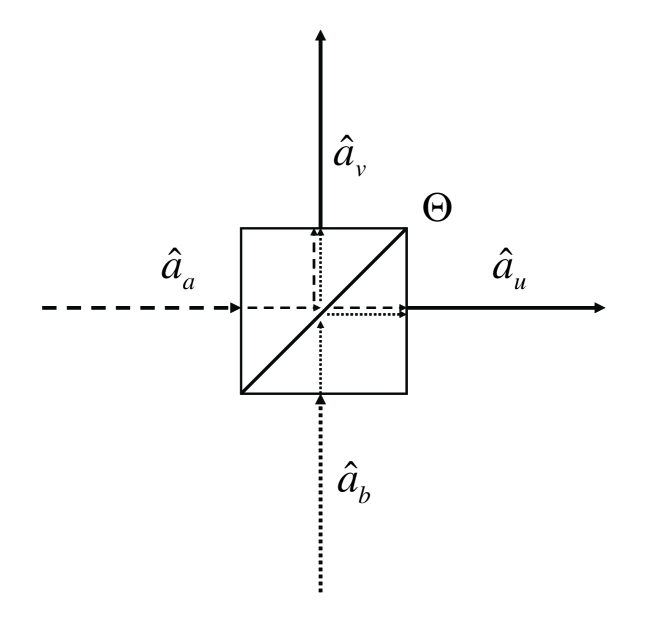
Figure 1.1: Geometric configuration of an ideal beam-splitter: The incoming modes $\hat{a}_{a}$ (dashed line) and $\hat{a}_{b}$ (dotted line) are ”mixed” by means of a partially reflecting surface of transmission coefficient $\cos(\Theta)$. The outcoming modes are $\hat{a}_{u}$ and $\hat{a}_{v}$; each consists in a linear combination of the reflected fraction of one mode and the transmitted fraction of the other mode.

Given two incoming modes represented by their annihilation operators in the Heisenberg interaction picture; $\hat{a}_{a}$ and $\hat{a}_{b}$, and the two outcoming modes’ operators $\hat{a}_{u}$, $\hat{a}_{v}$ as illustrated in fig. (1.1); the transformation effected by a lossless, phase-free beam-splitter is given by [2, 49]

$$\hat{a}_{u}= \;\widehat{B}_{ab}(\Theta)\;\hat{a}_{a}\;\widehat{B}^{{\dagger}}_{ab}(\Theta)$$

$$\hat{a}_{v}= \;\widehat{B}_{ab}(\Theta)\;\hat{a}_{b}\;\widehat{B}^{{\dagger}}_{ab}(\Theta)$$

$$\widehat{B}_{ab}(\Theta)= \;e^{\Theta\left(\hat{a}_{b}^{{\dagger}}\,\hat{a}_{a}\,-\,\hat{a}_{a}^{{\dagger}}\,\hat{a}_{b}\right)}$$ (1.24)

where the transmittance and reflectance coefficients of the beam-splitter apparatus are, respectively, $\cos^{2}(\Theta)$ and $\sin^{2}(\Theta)$. Given that $\widehat{B}_{ab}$ is an unitary transformation the commutation relations of $\hat{a}_{u}$ and $\hat{a}_{v}$ with their Hermitian conjugates and between their associated quadratures will be those of $\hat{a}_{a}$ and $\hat{a}_{b}$ and associated quadratures. The overall number of photons is conserved, as $\hat{n}_{u}+\hat{n}_{v}=\hat{n}_{a}+\hat{n}_{b}$.

Let us recall eq. (1.15); it is straightforward to re-state eq. (1.24) in the matrix form

$$\begin{pmatrix}\hat{a}_{u}\\ \hat{a}_{v}\end{pmatrix}=\begin{pmatrix}\cos(\Theta)&-\sin(\Theta)\\ \sin(\Theta)&\cos(\Theta)\end{pmatrix}\begin{pmatrix}\hat{a}_{a}\\ \hat{a}_{b}\end{pmatrix}$$ (1.25)

Given that $\hat{a}_{u,v}=\hat{x}_{u,v}+i\hat{p}_{u,v}$, the outcoming modes’ quadratures will be linear combinations of the incoming modes’ quadratures with an analogous relationship to that of eq. (1.25).

An operator that is an analytic function of the modes’ operators, such as $\widehat{F}(\hat{a}_{a},\hat{a}_{b}\,;\,\hat{a}^{{\dagger}}_{a},\hat{a}^{{\dagger}}_{b})$ will be transformed by eq. (1.25) onto

$$\widehat{F}^{\prime}(\hat{a}_{u},\hat{a}_{v};\hat{a}^{{\dagger}}_{u},\hat{a}^{{\dagger}}_{v})=\,\widehat{B}_{ab}(\Theta)\>\widehat{F}\>\widehat{B}^{{\dagger}}_{ab}(\Theta)=\widehat{F}(\hat{a}_{a}(\hat{a}_{u},\hat{a}_{v}),\,\hat{a}_{b}(\hat{a}_{u},\hat{a}_{v});\,\hat{a}^{{\dagger}}_{a}(\hat{a}^{{\dagger}}_{u},\hat{a}^{{\dagger}}_{v}),\,\hat{a}^{{\dagger}}_{b}(\hat{a}^{{\dagger}}_{u},\hat{a}^{{\dagger}}_{v}))$$ (1.26)

where $\hat{a}_{a,b}(\hat{a}_{u},\hat{a}_{v})$ denotes the inverse transform of eq. (1.25).

Most importantly, displacement operators for two separate modes $\widehat{D}_{a}(\alpha_{a})\>\widehat{D}_{b}(\alpha_{b})$ will be transformed to $\widehat{D}_{a}(\alpha_{a}(\alpha_{u},\alpha_{v}))\>\widehat{D}_{b}(\alpha_{b}(\alpha_{u},\alpha_{v})))=\widehat{D}_{u}(\alpha_{u})\>\widehat{D}_{v}(\alpha_{v})$. Where

$$\begin{pmatrix}\alpha_{u}\\ \alpha_{v}\end{pmatrix}=\begin{pmatrix}\cos(\Theta)&-\sin(\Theta)\\ \sin(\Theta)&\cos(\Theta)\end{pmatrix}\begin{pmatrix}\alpha_{a}\\ \alpha_{b}\end{pmatrix}$$ (1.27)

A separable two-mode state of radiation with a density matrix $\hat{\rho}_{a}\otimes\hat{\rho}_{b}$ entering the beam-splitter will be have, after the beam-splitter, a density matrix depending on modes’ operators $a_{u}$ , $a_{v}$ and their Hermitian conjugates. The resulting state will be usually [2] entangled, as the density matrix will not be factorized into two separate density matrices for the outcoming modes $u$ and $v$.

Consider for simplicity’s sake the separate wave function for a pure state $\psi_{a}(x_{a})\psi_{b}(x_{b})$; after the beam-splitter transformation it becomes (according to eq. (1.25)) equal to $\psi_{a}(x_{a}(x_{u},x_{v}),x_{b}(x_{u},x_{v}))$. The limit case for the entangled states achievable by beam-splitter interaction in quantum optics illustrates the point nicely; assume $\psi{a}(x_{a})=e^{2ix_{a}p^{\prime}}$, a position eigenstate, and $\psi_{b}(x_{b})=\delta(x_{b}-x^{\prime})$ a momentum eigenstate. After the beam-splitter transformation the joint wave function is

$$\delta\left((\cos(\Theta)\,x_{v}\,-\,\sin(\Theta)\,x_{u})\,-\,x^{\prime}\,\right)\;e^{2i\left(\cos(\Theta)\,x_{u}\,+\,\sin(\Theta)\,x_{v}\right)\,p^{\prime}}$$ (1.28)

which, for $\Theta=\pi/4$ and for the modes $u$ and $v$ is the wave function of the maximally entangled state in a CV setting, the EPR state [45]. That this state is maximally entangled can be seen easily; it is a joint eigenstate of the continuous, nonlocal quadratures $2^{-1/2}(x_{v}-x_{u})$ and $2^{-1/2}(p_{u}+p_{v})$, with eigenvalues $x^{\prime}$ and $p^{\prime}$, respectively. While the measurements effected on one of the local quadratures, say $x_{u}$, will yield a random result $x^{(m)}_{u}$, with a constant probability for all the values of $x_{u}$; this same measurement will fix the value of $x_{v}=2^{1/2}x^{\prime}-x^{(m)}_{u}$.

It has been shown that the EPR state is physically unfeasible, unless for an infinitesimal normalization constant, the wavefunction of eq. (1.28) is also not square-integrable.

1.2.3 Homodyne detection

The procedure for homodyne detection of quadratures of the radiation field is the basic detection scheme of CV quantum information protocols; such as quantum teleportation [33, 50, 51, 52, 53] and quantum tomography [54, 55]. We will describe the experimental procedure for homodyne measurement and the simple projective measurement that (ideally) projects the mode thus detected onto an eigenstate of the measured quadrature.

The experimental scheme for balanced homodyne detection [56] is illustrated in fig. (1.2).

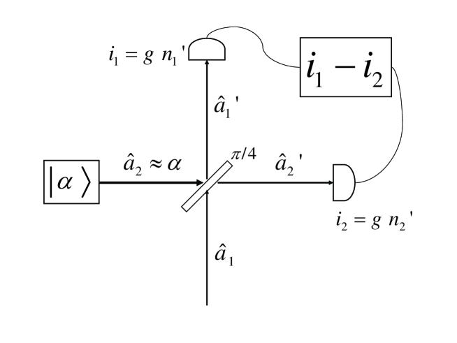
Figure 1.2: Idealized Homodyne Detection Scheme: Mode $\hat{a}_{1}$, to be measured, is mixed by means of a symmetric beam-splitter with mode $\hat{a}_{2}$, prepared in a coherent state $|\alpha\,\rangle$ of high intensity $|\alpha|^{2}$. Photo-detection is performed on modes $\hat{a}^{\prime}_{1}$ and $\hat{a}^{\prime}_{2}$. The photocurrents $i_{1}$ and $i_{2}$, proportional to the measured intensities, are subtracted to obtain a difference photocurrent that is proportional to the quadrature’s value.

Mode $\hat{a}_{1}$ is mixed with a reference mode $\hat{a}_{2}$ by means of a symmetric beam-splitter. Mode $\hat{a}_{2}$ is in a coherent state of a very high average photon number (light intensity), approximating a classical coherent source of light; it’s behavior can therefore be described approximately by it’s complex amplitude, thus $\hat{a}_{2}\approx\alpha=|\alpha|e^{i\Phi}$. The outcoming modes of the beam-splitter read

$$\hat{a}^{\prime}_{1}= \,2^{-1/2}(\,|\alpha|e^{i\Phi}\,+\,\hat{a}_{1})$$

$$\hat{a}^{\prime}_{2}= \,2^{-1/2}(\,|\alpha|e^{i\Phi}\,-\,\hat{a}_{1})$$ (1.29)

The intensity of the two outcoming modes is measured by photo-detectors (see fig. (1.2)), resulting in the photo-currents $i_{1}=\,g\langle\hat{a}_{1}^{{}^{\prime}{\dagger}}\hat{a}^{\prime}_{1}\rangle$ and $i_{2}=\,g\langle\hat{a}_{2}^{{}^{\prime}{\dagger}}\hat{a}^{\prime}_{2}\rangle$; which are proportional (with a known gain factor $g$) to the number of photons detected. Subtracting the photo-currents, we obtain

$$\delta\,i=\,i_{1}-i_{2}=\,g|\alpha|\langle\,e^{-i\Phi}\hat{a}_{1}+e^{i\Phi}\hat{a}_{1}^{{\dagger}}\,\rangle$$ (1.30)

The observable measured in eq. (1.30 is equal to $\hat{x}_{1}$ for $\Phi=0$ and is equal to $\hat{p}_{1}$ for $\Phi=\pi/2$. We can measure, controlling the phase of the reference coherent state $|\alpha\rangle$, a generalized quadrature of mode $1$;

$$\hat{x}_{1}^{(\Phi)}\equiv\,2^{-1}\left(e^{-i\Phi}\,\hat{a}_{1}\,+\,e^{i\Phi}\,\hat{a}_{1}^{{\dagger}}\right)$$ (1.31)

which would be identical to $\hat{x}_{1}$, for a phase shifted mode $1$ where $\hat{a}_{1}\rightarrow\hat{a}_{1}e^{-i\Phi}$. The conjugate quadrature to $\hat{x}_{1}$, satisfying the commutation relations in eq. (1.5 is simply $\hat{x}_{1}^{\Phi+\pi/2}$.

Ideally, the measurement of the quadrature $\hat{x}_{1}^{(\Phi)}$ on an arbitrary state $\rho_{1}$ of mode $1$ will obtain a random measurement result $x^{(\Phi)}$ and ”collapse” the state into the pure eigenstate $|x^{(\Phi)}\rangle_{1}$ of $\hat{x}_{1}^{(\Phi)}$. With a probability equal to

$$\mathrm{Tr}(\hat{\rho}_{1}|\,x^{(\Phi)}\rangle_{1}\langle\,x^{(\Phi)}|_{1})$$ (1.32)

thus, the system after the measurement can be said to be in a mixed state ; The pure components of the mixture being the $|x^{(\Phi)}\rangle_{1}$ eigenstates, with probability given by eq. (1.32).

To illustrate the concept of a projective measurement further, and particularly for two-mode states, let us consider a state with a density matrix $\hat{\rho}_{1,3}$. The state of mode $3$ after a projective measurement on mode $1$ obtaining a result $x^{(\Phi)}$ can be represented by a partial trace of the form

$$\mathrm{Tr}_{1}(\hat{\rho}_{1,3}|\,x^{(\Phi)}\rangle_{1}\langle\,x^{(\Phi)}|_{1})=\mathrm{P}(x^{(\Phi)})\hat{\rho}_{3}(x^{(\Phi)})$$ (1.33)

where $\mathrm{P}(x^{(\Phi)})$ is the probability density for the measurement result $x^{(\Phi)}$ when the quadrature $\hat{x}_{1}^{(\Phi)}$ is measured and $\hat{\rho}_{3}(x^{(\Phi)})$ is the state of mode $3$ after measurement. The operator of eq. (1.33 is not a normalized, proper density operator, because the ”projection” is not an unitary operation. It is easy to see also that the state of mode $3$ will not be affected by the measurement process on mode $1$ if the $\hat{\rho}_{1,3}$ state is separable into two density matrices; $\hat{\rho}_{1,3}=\hat{\rho}_{1}\otimes\hat{\rho}_{3}$. If $\hat{\rho}_{1,3}$ is an entangled, inseparable state; the state of mode $3$ after the measurement depends on the random outcome $x^{(\Phi)}$ of the measurement performed on mode $1$, with a probability $\mathrm{P}(x^{(\Phi)})$ for the state $\hat{\rho}_{3}(x^{(\Phi)})$. Such a state of ”classical ignorance” produced by measurement is a mixture of pure states. Therefore, we choose a properly normalized state for mode $3$, accounting for the random outcome of a projective measurement;

$$\hat{\rho}_{3}=\int dx^{(\Phi)}P(x^{(\Phi)})\hat{\rho}_{3}(x^{(\Phi)})=\int dx^{(\Phi)}\mathrm{Tr}_{1}(\hat{\rho}_{1,3}|\,x^{(\Phi)}\rangle_{1}\langle\,x^{(\Phi)}|_{1})$$ (1.34)

1.2.4 The one and two-mode squeezing operator and the squeezed states

Producing physically feasible states approximating as an asymptotic limit the position (or momentum) eigenstates, that can then be entangled by a beam-splitter requires interactions of a finite energy that cause these states to have a narrower position (or momentum) wave function and a wider momentum (or position) wave function. Though any state that has a different variance for position and momentum can be thought of as squeezed, we will generally term squeezed states those that have been transformed by a particular kind of unitary evolution named the squeezing transformation.

To effect such an evolution in the laboratory requires the use of nonlinear optical elements and optical pumping [57, 58]. The simplest example of an squeezing evolution involves the use of a nonlinear medium down-converting photons of a given frequency to two photons of half this frequency [43, 58]. Let $\hat{a}$ be the annihilation operator for the mode to be squeezed, of frequency $\hbar\omega$. Let $\hat{b}$ be the annihilation operator for an intense coherent field; the pump, of frequency $2\hbar\omega$. Let $\Xi^{(2)}$ be the strength of the coupling between the two modes, and the nonlinear coefficient of the medium inside which the squeezing evolution occurs. For a lossless setup the Hamiltonian for the interaction is given by

$$\widehat{H}_{I}=2^{-1}\>i\>\hbar\>\Xi^{(2)}\,(\hat{b}^{{\dagger}}\,\hat{a}^{2}\,-\,\hat{b}\,\hat{a}^{{\dagger}\,2}\,)$$ (1.35)

For each photon of the pump annihilated, two photons of the mode are created, and viceversa. Given the high intensity of the pump field and its quasi-classical character, it’s annihilation operator can be approximated by a complex amplitude, $\hat{b}\approx\beta$.

The unitary evolution operator, $U(t)=e^{-i\hbar^{-1}\widehat{H}_{I}\,t}$ for the time independent Hamiltonian in eq. (1.35) will therefore be

$$\widehat{S}(\zeta)\,=\,e^{\,\frac{1}{2}\,\left(\zeta^{*}\,\hat{a}^{2}\,-\,\zeta\,\hat{a}^{{\dagger}2}\right)}$$ (1.36)

with $\zeta=\Xi^{(2)}\,\beta\,t$, the phase of argument of the operator being that of the pump field. This evolution operator is unitary, therefore $\widehat{S}(-\zeta)=\widehat{S}^{{\dagger}}(\zeta)=\widehat{S}^{-1}(\zeta)$.

$\widehat{S}(\zeta)$ has been named the squeezing operator [43, 47], having a complex argument $\zeta=|r|\,e^{i\varphi}$. The modulus  of this argument, $|r|$, usually called the squeezing coefficient is a characteristic interaction time and a logarithmic measure of the degree of squeezing. The squeezing phase $\varphi$, equal to that of the pump field, will determine the phase-space orientation of the squeezing transformation.

Using the ordering identities of eqs. (1.5) and (1.15), the results of the squeezing transformation on annihilation and creation operators, and on the displacement operator can be derived,

$$\widehat{S}(\zeta)\,\hat{a}\,\widehat{S}^{{\dagger}}(\zeta)= \,\hat{a}\,\cosh(r)\,-\,\hat{a}^{{\dagger}}\,\sinh(r)\,e^{i\varphi}$$

$$\widehat{S}(\zeta)\,\hat{a}^{{\dagger}}\,\widehat{S}^{{\dagger}}(\zeta)= \,\hat{a}^{{\dagger}}\,\cosh(r)\,-\,\hat{a}\,\sinh(r)\,e^{-i\varphi}$$

$$\widehat{S}(\zeta)\,\widehat{D}(\,\alpha)\,\widehat{S}^{{\dagger}}(\zeta)= \,\widehat{D}(\alpha\,\cosh(r)\,-\,\alpha^{*}\,\sinh(r)\,e^{i\varphi}\,)$$ (1.37)

Given eqs. (1.31) and (1.37), the result of the squeezing transformation of the generalized quadrature $\hat{x}^{(\Phi)}$ can be calculated;

$$\widehat{S}(\zeta)\;\hat{x}^{(\Phi)}\;\widehat{S}^{{\dagger}}(\zeta)=\,-e^{r}\,\sin(\Phi-\varphi/2)\>\hat{x}^{(\varphi/2+\pi/2)}\,+\,e^{-r}\,\cos(\Phi-\varphi/2)\>\hat{x}^{(\varphi/2)}$$ (1.38)

Taking $\Phi=\varphi/2$; the expression in eq. (1.38) is simplified as the phase orientation of the quadrature $\hat{x}^{(\Phi)}$ coincides with the phase orientation of the squeezing operator. Thus we have,

$$\widehat{S}(r\,e^{2i\Phi})\;\hat{x}^{(\Phi)}\;\widehat{S}^{{\dagger}}(r\,e^{2i\Phi})= \,e^{-r}\,\hat{x}^{(\Phi)}$$

$$\widehat{S}(r\,e^{2i\Phi})\;\hat{x}^{(\Phi+\pi/2)}\;\widehat{S}^{{\dagger}}(r\,e^{2i\Phi})= \,e^{r}\,\hat{x}^{(\Phi+\pi/2)}$$

$$\Delta(\widehat{S}(r\,e^{2i\Phi})\;\hat{x}^{(\Phi)}\;\widehat{S}^{{\dagger}}(r\,e^{2i\Phi}))^{2}= \,e^{-2r}\,\Delta(\hat{x}^{(\Phi)})^{2}$$

$$\Delta(\widehat{S}(r\,e^{2i\Phi})\;\hat{x}^{(\Phi+\pi/2)}\;\widehat{S}^{{\dagger}}(r\,e^{2i\Phi}))^{2}= \,e^{2r}\,\Delta(\hat{x}^{(\Phi+\pi/2)})^{2}$$ (1.39)

For $r>0$, the variance of $\hat{x}^{(\Phi)}$ is scaled by a factor of $e^{-2r}$ and the associated wavefunction is made narrower; this is termed squeezing in the language of quantum optics. While the opposite happens to the conjugate quadrature $\hat{x}^{(\Phi+\pi/2)}$, ”expanded” by the inverse factor $e^{2r}$. Thus the squeezing transformation preserves the product of variances in Heisenberg’s uncertainty relation, eq. (1.11). A quantum state for which that product is equal to the lower bound of $\frac{1}{16}$, a minimum uncertainty state, will continue to be of minimum uncertainty after being ”squeezed”.

With the purpose of simplifying calculations, we will take the squeezing operator’s argument to be real; $\zeta=r$, where $r$ can be negative. This is equivalent to the choice made for eq. (1.39) of squeezing phase-orientation; on quadratures $\hat{x}^{(0)}$ and $\hat{p}=\hat{x}^{(\pi/2)}$.

The states usually associated with the squeezing operator $\widehat{S}(\zeta)$ are the coherent squeezed states [47, 59], produced by the squeezing transformation of a vacuum state; on which is then performed a displacement operation. Consider the case where $\Phi=\varphi=0$;

$$|\alpha;r\,\rangle=\widehat{D}(\alpha)\>\widehat{S}(r)|0\,\rangle$$ (1.40)

The coherent squeezed states are minimum uncertainty states like the coherent states, with the variance $\Delta\hat{x}^{2}=e^{-2r}/4$ reduced and $\Delta(\hat{p}^{2}=e^{2r}/4$ increased when $r>0$. When $r<0$, which corresponds to $\varphi=\pi$, the $\hat{p}$ quadrature is the one ”squeezed” and it’s variance is reduced. The wave function in either basis of representation is Gaussian, and the averages of position and momentum are, respectively, the real and imaginary part of $\alpha$.

The infinite squeezing (and coupling $\times$ intensity of pump $\times$ time, as $r=|\beta|\xi^{(2)}t$) limit for the squeezed states $\widehat{S}(re^{i\varphi})$ are the $\hat{x}^{(\varphi/2)}$ quadrature eigenstates. In such a way a physically feasible approximation for a quadrature eigenstate can be obtained by appropriate squeezing of an initial coherent state where $\alpha$ is wholly real (position eigenstate, $r>0$) or imaginary (momentum eigenstate, $r<0$), the limitation being technological.

Quantum state preparation approximating the maximally entangled EPR states is possible given strong nonlinear interactions, control of the phase of the individual modes, and beam-splitters (see eqs. (1.25), (1.26) and (1.28)). Two coherent squeezed states, squeezed in position and in momentum can be mixed by a beam-splitter obtaining a Gaussian state ”squeezed” in nonlocal quadratures. Which, in the limit $r\,\rightarrow\,\infty$ becomes an EPR state.

The operation described above can be represented by the Two-mode squeezing operator [47]. Two-mode squeezing is the transformation preparing an entangled, symmetric Gaussian state state; from a two mode vacuum state vector $|\,0\rangle\_{1},\otimes\,|\,0\rangle_{2}$:

$$\widehat{S}_{12}(\zeta)=e^{-\zeta\hat{a}_{1}^{{\dagger}}\hat{a}_{2}^{{\dagger}}+\zeta\hat{a}_{1}\hat{a}_{2}}\;\;\;\;\;\;\;\zeta\equiv\,r\,e^{i\phi}$$ (1.41)

It is straightforward to show that the two-mode squeezing operator can be written as the product of two squeezing operators for different modes and a beam-splitter transformation;

$$\widehat{S}_{12}(r)\equiv\,\widehat{B}_{12}(\pi/4)\>\widehat{S}_{1}(r)\>\widehat{S}_{2}(-r)$$ (1.42)

where the two squeezing operations represent the nonlinear interaction (see eqs. (1.35) and (1.36)) transforming each of the initial vacuums into states squeezed, respectively, in the quadratures $\hat{x}_{1}$ and $\hat{p}_{2}$. The symmetric beam-splitter transformation mixes the two squeezed states (see eq. (1.28) and discussion above) into an approximate EPR state, the two-mode squeezed vacuum; $|\zeta\rangle_{AB}$.

Recalling the beam-splitter transformation’s operation on a two-mode quantum state wavefunction, it is easily seen that the two mode-squeezed vacuum is Gaussian in wavefunction. The two-mode squeezed vacuum is an entangled state, and correlations arise in the measurement of observables other than the nonlocal quadratures. In the Fock state basis representation;

$$|r\,\rangle_{12}=\,(\cosh(r))^{-1}\sum_{n=0}^{\infty}\left(\,\tanh(r)\,\right)^{n}\;|n\rangle_{1}\;|n\rangle_{2}$$ (1.43)

The state vector is symmetric under exchange of modes $1$ and $2$, having an even overall number of photons. A measurement of photon number must give the same result for modes $1$ and $2$. For the two-mode squeezed state $\langle\,\hat{n}_{1}-\hat{n}_{2}\rangle=0$, even if the overall photon number $n_{1}+n_{2}$ is not unambiguously defined.

The factor $(\tanh(r))^{n}$ in eq. (1.43) makes for a probability of measuring (overall) $2\;n$ photons that decreases exponentially with $2n$; and ensures the convergence of the infinite sum for finite $r$. The infinite squeezing limit $r\rightarrow\infty$ of eq. (1.43) is the EPR state of eq. (1.28). In this limit the infinite sum does not converge and the normalization constant $(\cosh{r})^{-1}$ becomes infinitesimal.

To study the effect of two-mode squeezing on non-Gaussian states’ wave functions and phase-space representations; it suffices to study the transformation of modes’ operators $\hat{a}_{1}$ and $\hat{a}_{2}$;

$$\widehat{S}_{12}(\zeta)\,\hat{a}_{i}\,\widehat{S}_{12}^{{\dagger}}(\zeta)=\cosh(r)\,\hat{a}_{i}-e^{i\phi}\sinh(r)\,\hat{a}_{j}^{{\dagger}}\;\;\;\;\hbox{for}\;\;i\neq j=1,2$$ (1.44)

a Bogoliubov transformation mixing mode operators.

Analytic functions of the operators $\hat{a}_{1,2},\hat{a}_{1,2}^{{\dagger}}$ will be transformed in an analogous manner to that of eq. (1.25); with the Bogoliubov transformation of eq. (1.44) substituting for the beam-splitter transformation. An interesting and useful (for the purposes of this work) example is that of a product of displacement operators in two modes,

$$\widehat{S}_{12}(\zeta)\;\widehat{D}_{1}(\alpha_{1})\;\widehat{D}_{2}(\alpha_{2})\;\widehat{S}^{{\dagger}}_{12}(\zeta)=\widehat{D}_{1}(\alpha^{\prime}_{1})\;\widehat{D}_{2}(\alpha^{\prime}_{2})$$ (1.45)

$$\alpha^{\prime}_{i}=\>\cosh(r)\,\alpha_{i}\,+\,e^{i\phi}\sinh(r)\,\alpha_{j}^{*}\;\;\;\hbox{for}\;\;i\neq j=1,2$$ (1.46)

1.3 The Wigner and the Wigner characteristic function

In this section, we introduce phase-space representations; of quantum states’ density matrices, and of any square-integrable operator [46]. In particular, we introduce the Wigner function [60] and the Wigner characteristic function [46] as particularly useful for the representation of CV systems because they are explicit, analytic functions of phase-space ”coordinates” that transform in the same manner as the wave functions of quantum states [48]. Though the Wigner function is not a genuine probability distribution in momentum and position, the two conjugate functions allow the calculation of quantum mechanical averages, including partial traces, to take the form of integrals over the complex plane of phase-space. Unitary evolutions and measurements over a multi-mode quantum state likewise take the form of simple unitary transformations on the arguments of the functions, and projections on adequate eigenstates.

1.3.1 Phase-space representations: mainly Wigner function and characteristic function

The Wigner function was proposed and chosen to be an Hermitian form (real scalar) of the density operator of a quantum state fulfilling a number of desirable conditions; to be real and bounded, to transform according to the same rules for a classical distribution of probability; to produce the quantum mechanical averages pertaining to the density operator [48]; to give the appropriate probability distributions when integrated. Such a function was proposed in ref. [60] in the form

$$W(\alpha\,=\,x+ip)=\int dy\;\langle\,x-\frac{y}{2}|\,\hat{\rho}\,|x+\frac{y}{2}\,\rangle\>e^{2ipy}$$ (1.47)

with the unit system defined so $\hbar=\frac{1}{2}$. The Wigner function is real, and can be demonstrated to exist and be square-integrable for any density operator [46]. It has been termed a pseudo-distribution and as such, a conjugate function, it’s Fourier transform, the Wigner characteristic function has been defined [48];

$$\chi(\xi)= \,\pi^{-1}\,\int d^{2}\,\alpha\>e^{\xi\alpha^{*}-\xi^{*}\alpha}\;W(\alpha)$$ (1.48)

$$W(\alpha)= \,\pi^{-1}\,\int d^{2}\,\xi\>e^{\alpha\xi^{*}-\alpha^{*}\xi}\;\chi(\xi)$$ (1.49)

with $\xi=w+iz$ being a conjugate phase-space ”coordinate”. The characteristic function for a density operator, being the Fourier transform of the analytic, real Wigner’s function is thus an analytic function. We remark here that ”Wigner” representations of suitable operators other than the density operators can be calculated, and are necessary to the calculation of physicalle relevant quantum mechanical averages using this representation.Let us review the forms (in a strict mathematical sense) corresponding to quantum mechanical averages and normalization conditions.

The normalization condition on density operators; $\mathrm{Tr}(\hat{\rho})=1$ is equivalent, in the Wigner and Characteristic Function descriptions to

$$\mathrm{Tr}(\hat{\rho})=\pi^{-1}\,\int d^{2}\,\xi\;\chi_{\rho}(\xi)=\pi^{-1}\,\int d^{2}\,\alpha\;W_{\rho}(\alpha)\,=\,1$$ (1.50)

Finite Wigner function and characteristic functions can be derived, and used to calculate quantum mechanical averages for any operator fulfilling the condition that the Hilbert-Schmidt norm $\mathrm{Tr}(\widehat{F}^{{\dagger}}\widehat{F})$ be finite, in other words that the operator be bounded [46]. The density operators are, furthermore, trace-class operators with trace equal to $1$; therefore $\mathrm{Tr}(\hat{\rho}^{2})\leq 1$, and

$$\mathrm{Tr}(\hat{\rho}^{2})\,=\,\pi^{-1}\>\int d^{2}\,\xi\;|\chi_{\rho}(\xi)|^{2}\,=\,\pi^{-1}\>\int d^{2}\,\alpha\;|W_{\rho}(\alpha)|^{2}\,\leq\,1$$ (1.51)

The quantity $\mathrm{Tr}(\hat{\rho}^{2})$ is a quantitative measure of the purity of the quantum state, and is thus named.

Quantum mechanical averages or expectation values of the product of at least one trace-class operator and a bounded operator are finite and are given by the form $\mathrm{Tr}(\widehat{F}\widehat{G})$;

$$\mathrm{Tr}(\widehat{F}\,\widehat{G})\,=\, \pi^{-1}\>\int d^{2}\,\xi\;\chi_{F}(\xi)\;\chi_{G}(-\xi)$$ (1.52)

$$=\, \pi^{-1}\,\int d^{2}\,\alpha\;W_{F}(\alpha)\;W_{G}(\alpha)$$ (1.53)

where $W_{F},W_{G}$ and $\chi_{F},\chi_{G}$ are the Wigner and characteristic functions corresponding to $\widehat{F},\widehat{G}$ respectively.

The Wigner function can be easily shown not to be a genuine probability distribution for density operators, even though it produces expectation values and is normalized to $1$ like a classical probability distribution. Let $\hat{\rho}_{\Phi}=\,|\Phi\rangle\,\langle\Phi|$ and $\hat{\rho}_{\Psi}=\,|\Psi\rangle\,\langle\Psi|$, density operators for two pure states. If the states are orthogonal, then $\langle\,\Phi\,|\,\Psi\,\rangle=\,\mathrm{Tr}(\hat{\rho}_{\Phi}\>\hat{\rho}_{\Psi})\,=\,0$. The integral of the product of two nonzero Wigner functions in eq. (1.53) is equal to zero. Hence, the Wigner function of at least one of the density operators must have negative values. The Wigner function cannot be a genuine probability distribution for all quantum states, and is thus termed a pseudo-probability. Conversely, quantum states with a positive Wigner function that is a genuine probability distribution cannot be orthogonal with each other.

Quantum states of a nonclassical character have a Wigner function [11, 13] with negative values in parts of its domain; the negative volume of the Wigner function has been proposed as a measure of the nonclassical character of a quantum state [61].

The Wigner characteristic function is the trace of the product of the density operator and the displacement operator [46, 48]; the mean value of the displacement operator for the density $\hat{\rho}$. Recall that displacement operators form an orthogonal basis for the representation of square-integrable operators (see eq. (1.23) and that any bounded operator may be represented by a linear combination of displacement operators [46]. The characteristic function is the coefficient for this representation, and is necessarily square-integrable (see eq. (1.51)) when the operator itself is trace-class. The characteristic function is also given by

$$\chi(\xi)=\,\mathrm{Tr}(\,\hat{\rho}\,\widehat{D}(\xi)\,)$$ (1.54)

which for a pure state $\hat{\rho}=\,|\psi\rangle\,\langle\psi|$ becomes

$$\chi(\xi)=\,\langle\,\psi\,|\>\widehat{D}(\xi)\>|\,\psi\,\rangle$$ (1.55)

Generalizing the characteristic function to more than one mode is straightforward; the product of operators to be traced over in eq. (1.54) being that of the density operator and the commuting displacement operators $\widehat{D}_{1}(\xi_{1})\>\widehat{D}_{2}(\xi_{2})\ldots\widehat{D}_{N}(\xi_{N})$, for $N$ modes.

A most important property of the characteristic function, is that transformations on density operators of quantum states such as those we have reviewed in the preceding section will correspond, in the language of the characteristic functions, to transformations on the arguments $\xi_{i}$ of the displacement operators (see eqs. (1.27), (1.18), (1.37) and (1.46)); which are the arguments of the characteristic function.

The Wigner function and Wigner characteristic function are associated to a symmetric ordering of operators [46, 48]; where ordering means the left to right ordering of the non-commuting $\hat{a}$ and $\hat{a}^{{\dagger}}$ operators inside other operators such as density matrices and observables. For example: the number operator $\hat{n}=\hat{a}^{{\dagger}}\hat{a}$ is symmetrically ordered as $2^{-1}(\hat{a}^{{\dagger}}\hat{a}+\hat{a}\hat{a}^{{\dagger}})$, normally ordered as $\hat{a}^{{\dagger}}\hat{a}$, anti-normally ordered as $\hat{a}\hat{a}^{{\dagger}}$.

Other phase-space representations exist based on alternative orderings. In the manner discussed above, the $P(\alpha)$ [38] representation and the $Q(\alpha)$ [62] function are conjugate with characteristic functions associated with the normal and anti-normal ordering of operators, respectively. Particularly, with the ordering of the displacement operator of which the characteristic function is a coefficient of representation;

$$\{\widehat{D}(\xi)\}=\, e^{\xi\hat{a}^{{\dagger}}-\xi^{*}\hat{a}}$$

$$\widehat{D}(\xi,s)=\, e^{s|\xi^{2}|/2}\{\widehat{D}(\alpha)\}$$

$$\widehat{D}(\xi,1)=\, e^{\xi\hat{a}^{{\dagger}}}\>e^{-\xi^{*}\hat{a}}$$

$$\widehat{D}(\xi,-1)=\, e^{-\xi^{*}\hat{a}}\>e^{\xi\hat{a}^{{\dagger}}}$$ (1.56)

where the index takes the values $s=1$ for normal ordering, $s=0$ for symmetric ordering, also denoted by the brackets $\{\ldots\}$, and $s=-1$ for antinormal ordering. It is obvious from inspection of eq. (1.54) and eq. (1.56) that the transformation between characteristic functions associated with different orderings is just a power of $e^{|\xi^{2}|/2}$.

The characteristic function of the Wigner distribution, similarly to a classical characteristic function, is the generating function for the symmetrically ordered moments of annihilation and creation operators [47];

$$\langle\left\{\,(\hat{a}^{{\dagger}})^{m}\,\hat{a}^{n}\,\right\}\rangle=\,\mathrm{Tr}(\hat{\rho}\,\left\{(\hat{a}^{{\dagger}})^{m}\,\hat{a}^{n}\,\right\})\,=\,\left.\left(\,\frac{\partial}{\partial\xi}\right)^{m}\left(-\frac{\partial}{\partial\xi^{*}}\right)^{n}\,\chi(\xi)\;\right|_{\>\xi\,=\,\xi^{*}\,=\,0}$$ (1.57)

simplifying the calculation of statistical moments; specially quantum mechanical averages and covariances.

1.3.2 Characteristic functions of the two-mode squeezed vacuum and EPR states

The characteristic function for a Gaussian, two-mode squeezed vacuum state $|0\rangle_{a}\otimes|0\rangle_{b}$ is given by

$$\chi_{S}(\xi_{a},\xi_{b})\,=\,e^{-1/2\left(|\xi^{\prime}_{a}|^{2}\,+\,|\xi^{\prime}_{b}|^{2}\right)}$$ (1.58)

where the relation of the pair of variables $\xi^{\prime}_{a},\xi^{\prime}_{b}$ to the pair of variables $\xi_{a},\xi_{b}$ is the Bogoliubov transformation described in eq. (1.46). Other, displaced two-mode coherent states have a characteristic function similar to the one in eq. (1.58) with a multiplying phase factor. For an overall phase-space displacement of, say $x^{\prime}\,+\,ip^{\prime}$ on $A$ mode this factor is given by $e^{2i(z_{a}\,x^{\prime}\>-\>w_{a}\,p^{\prime})}$.

The infinite squeezing limit of the Gaussian two-mode squeezed state is the EPR state. In a CV setting, it is the maximally entangled state [45] of two nonlocal quadratures $x_{u},p{v}$, as defined by the unitary transformation of eq. (1.27). Given the wave function (see eq. (1.28)), the Wigner function of the state can be derived easily from it’s definition in eq. (1.47),

$$W_{x^{\prime}_{u},p^{\prime}_{v}}(\alpha_{a}\,,\,\alpha_{b})\,=\,\mathcal{C}\;\delta(\cos(\Theta)\,x_{a}\,-\,\sin(\Theta)\,x_{b}\,-\,x^{\prime}_{u})\;\delta(\sin(\Theta)\,p_{a}\,+\,\cos(\Theta)\,p_{b}\,-\,p^{\prime}_{v})$$ (1.59)

where $\mathcal{C}$ is a normalization factor that becomes infinitesimally small as $r\rightarrow\infty$. The characteristic function of the EPR state is easy to calculate as the Fourier transform (eq. (1.48)) of eq. (1.59);

$$\chi_{x^{\prime}_{u},p^{\prime}_{v}}(\xi_{a},\xi_{b})\,=\,\mathcal{C}\;\delta(z_{a}\,\sin(\Theta)\,+\,z_{b}\,\cos(\Theta))\;\delta(w_{a}\,\cos(\Theta)\,-\,w_{b}\,\sin(\Theta))\>e^{2i(z_{a}\,x^{\prime}_{u}\,\sec(\Theta)\,-\,w_{a}\,p^{\prime}_{v}\,\csc(\Theta))}$$ (1.60)

which is, again, not square-integrable. However, the product of this characteristic function and a square-integrable characteristic function can be traced over (integrated) in the manner of eq. (1.52).

1.4 Universal quantum teleportation (in Continuous Variables)

This section will review both the universal protocol for Quantum Teleportation of a quantum state (and apply it to a CV setting) and the fidelity of teleportation in the language of Wigner characteristic functions.

1.4.1 Quantum teleportation

The quantum teleportation protocol involves the transcription of the unknown quantum state of a physical system $in$ (named input) onto the quantum state of another, similar physical system $B$  that is remote with respect to $in$. The protocol itself is a projective measurement of the maximally entangled states for that setting [25, 26, 63], the Bell states (in Continuous Variables the EPR states) on the joint system consisting on state $in$ and another, similar system $A$ .

Quantum teleportation is not ”cloning” the quantum state, as this operation is impossible for arbitrary states [64]. It is no scheme of quantum measurements on the input state or of repeated measurements on identical instances of preparation as is done in quantum tomography [65, 66]. The state itself is unknown and is to remain unknown through teleportation; in principle there is only one copy available for teleportation.

The transcription of an unknown state from $in$ to physically separate system $B$ by measurements on systems $A$ and $in$ is only possible if a quantum correlation exists between the states of the two systems $A$ and $B$ (the joint, entangled state of both being named resource) and if a correlation is forced on the $A,in$ state by interaction between the two systems before measurement; there is no Bell state measurement without previous interaction [67].

An obvious maximally entangled or Bell state for a quantum system Hilbert space $\mathcal{H}$ of dimensionality $d$ can be formulated with ease [26]. Let $\{|n\rangle\}$ be a complete basis of representation of $\mathcal{H}$; the simplest Bell state has a state vector

$$|\Psi_{0}\,\rangle_{AB}\,=\,d^{-1/2}\>\sum_{n}\>e^{-i\phi_{n}}\;|\,n\,\rangle_{A}\;|\,n\,\rangle_{B}$$ (1.61)

belonging to the joint Hilbert space $\mathcal{H}\otimes\mathcal{H}$. This state has the same form when written in terms of any complete basis of representation of $\mathcal{H}$. Let the basis $\{|n\rangle\}$ be made of eigenstates of an observable operator $\hat{n}$; Alice’s measurement of $\hat{n}_{A}$ will determine the result for Bob’s measurement of $\hat{n}_{B}$. It follows, on inspection, that the Bell state of eq. (1.61) is an eigenstate of nonlocal observable $\hat{n}_{A}-\hat{n}_{B}$ with eigenvalue $0$. nonlocal observables having as eigenstates the maximally entangled Bell states are termed Bell observables; their measurement is taken to be a projective measurement of the Bell state . Note that the squeezed vacuum of eq. (1.43) and its infinite squeezing limit, the EPR state of CV systems  are eigenstates of a nonlocal observable (the difference in photon number of the two systems).

Other maximally entangled eigenstates, associated to other eigenvalues of Bell observables can be produced by a local unitary transformation on eq. (1.61);

$$|\Psi_{g}\rangle_{AB}=\,\widehat{U}_{A}(g)\;|\,\Psi_{0}\,\rangle_{AB}$$ (1.62)

In this case Alice has performed the operation $\widehat{U}(g)$. To produce all the possible Bell states, $\widehat{U}(g)$ must belong to a group of unitary transformations $\{\widehat{U}(g)\}$ having an irreducible unitary representation in the space of operators acting on $\mathcal{H}$. Schur’s lemma for the density operators of the Bell states takes the form:

$$\int dg\>\widehat{U}_{A}(g)\>|\,\Psi_{0}\,\rangle_{AB}\>\langle\,\Psi_{0}\,|_{AB}\>\widehat{U}_{A}^{{\dagger}}(g)\,=\,d^{-1}\;\hat{\mathbf{1}}_{A}\,\otimes\,\hat{\mathbf{1}}_{B}$$ (1.63)

with the integration over the argument $g$ being replaced by a sum whenever the group is discrete. The factor $d^{-1}$ becomes infinitesimal for CV systems.

The identity in eq. (1.63) is a proof that the group consisting of density operators of Bell states form a Positive Operator Valued Measure [25] (abbreviated POVM). It is also a proof that the Bell states form a complete, orthonormal basis for the Hilbert space $\mathcal{H}\otimes\mathcal{H}$; eq. (1.63) is a completeness relationship for Bell basis states.

For the $2$-dimensional (spin $1/2$) Hilbert space of the original teleportation proposal [81], the unitary transformation group consists in the set of the Pauli operators $\left\{\,\hat{\mathbf{1}}\,,\,\hat{\sigma}^{(x)}\,,\,\hat{\sigma}^{(y)}\,,\,\hat{\sigma}^{(z)}\,\right\}$. The Bell basis is given by

$$|\uparrow\,\rangle_{A}\,|\uparrow\,\rangle_{B}\;+\;e^{i\Theta}\,|\downarrow\,\rangle_{A}\,|\downarrow\,\rangle_{B}$$

$$|\uparrow\,\rangle_{A}\,|\downarrow\,\rangle_{B}\;+\;e^{i\Theta}\,|\downarrow\,\rangle_{A}\,|\uparrow\,\rangle_{B}$$ (1.64)

with $\Theta=0,\pi$. The Bell observables are given by

$$\hat{\sigma}^{(z)}_{A}\,-\,\hat{\sigma}^{(z)}_{B}$$

$$\hat{\sigma}^{(z)}_{A}\,+\,\hat{\sigma}^{(z)}_{B}$$ (1.65)

In a CV setting a $2$-dimensional Hilbert space (of bosonic excitations, though) can be defined by a truncation of the Fock basis to the first two states $\{|0\rangle,|1\rangle\}$. The most general superposition state for this truncated space is of the form $\cos(\varepsilon)\,|\,0\,\rangle\>+\>e^{i\Theta}\,\sin(\varepsilon)\,|\,1\,\rangle$. The Bell observables are $\hat{n}_{A}-\hat{n}_{B}$ and $\hat{n}_{A}+\hat{n}_{B}$ and their eigenstates have a form similar to that of eq. (1.64).

For a full CV setting the group of unitary transformations producing the Bell states is that of the displacement operators and the Bell basis is made of the EPR states of eq. (1.28). The state in eq. (1.61) being the infinitely squeezed two-mode vacuum (see eq. (1.43)); having nonlocal quadratures’ (Bell observables) eigenvalues $\hat{p}_{A}+\hat{p}_{B}=0$ and $\hat{x}_{A}-\hat{x}_{B}=0$. The displacement operation, when performed by either Alice or Bob will produce all the other possible values for the nonlocal quadratures. The POVM for the Bell-basis measurement of Bell operators will be the homodyne measurement POVM [63].

For the quantum teleportation protocol, we have a three-party joint system of the entangled resource $AB$, and the input $in$ with a density operator $\hat{\rho}_{in}\otimes\hat{\rho}_{AB}$. The teleportation protocol consists in the measurement of the Bell observables (projective measurement of the Bell states) over the modes $A,in$ in Alice’s possession.

Given the POVM defined in eq. (1.63), a measurement with a definite result $g$ would result in a state, after measurement (see eqs. (1.32), (1.33) and (1.34) and the associated discussion of projective measurements);

$$\mathrm{Tr}\left(\,\hat{\rho}_{in}\,\otimes\,\hat{\rho}_{AB}\>|\,\Psi_{g}\,\rangle_{in,A}\>\langle\,\Psi_{g}\,|_{in,A}\,\right)_{A,in}$$ (1.66)

which is generally not normalized. To simplify and restrict exposition to Bell resource teleportation, let the input state be the pure state $|\psi\rangle_{in}$; let the resource be $|\Psi_{0}\rangle_{AB}$ of eq. (1.61); lastly, let the basis of representation for the states $\{|\,n\,\rangle\}$ be orthonormal. The outcome of the projective measurement of eq. (1.66) with a result $g$ is the state

$$d^{\,-1}\>\sum_{n,n^{\prime}}\,e^{i\,\phi_{n^{\prime}}\,-\,i\,\phi_{n}\,}\>\langle\,n^{\prime}\,|_{A}\>\langle\,n^{\prime}\,|_{in}\;\widehat{U}_{in}^{{\dagger}}(g)\;\;|\,n\,\rangle_{A}\>|\,n\,\rangle_{B}\>|\,\psi\,\rangle_{in}=\,d^{\,-1}\>\sum_{n}\>\langle\,n\,|\>\widehat{U}^{{\dagger}}(g)\>|\,\psi\,\rangle\>|\,n\,\rangle_{B}$$ (1.67)

Given the complete and orthonormal nature of the basis $\{|\,n\,\rangle\}$; the state in eq. (1.67) is the original input state (now ”living” in system $B$ instead of $in$), on which the transformation $\widehat{U}^{{\dagger}}(g)$ has been performed.

Note that the Bell state for the outcome of measurement $g$ and the resource state are related by the transformation $|\Psi_{g}\rangle_{AB}=\widehat{U}_{A}(g)|\Psi_{0}\rangle_{AB}$. Moreover, the generalization to a teleportation protocol where the resource state is a Bell state different from $|\Psi_{0}\rangle_{AB}$ is straightforward; as $\{\widehat{U}(g)\}$ is a group, with a group composition law:

$$\widehat{U}(g^{\prime})\>\widehat{U}(g^{\prime\prime})\,=\,\widehat{U}(g^{\prime}\cdot g^{\prime\prime})\>e^{i\Phi(g^{\prime},g^{\prime\prime})}$$ (1.68)

where $e^{i\Phi(g^{\prime},g^{\prime\prime})}$ is a phase factor (f.e. the phase in eq. (1.18) for displacements); and the operation indicated by $g^{\prime}\cdot g^{\prime\prime}$ is algebraic. The phase factor and the arguments $g$ under the operation $\cdot$ are associative, with an inverse element and an identity element. Thus, the transformations on a Bell state not equal to $|\Psi_{0}\rangle_{AB}$ can be compounded with ease.

To finish the teleportation protocol, Bob must apply the transformation $\widehat{U}_{B}(g)$ onto the state $B$ in his possession. The result of measurement is random in a fundamental manner; to know which transformation to apply Bob has to receive a communication from Alice via a classical communication channel.

Owing to the random nature of projective measurement, Bob’s output state should in reality be an ensemble of all the possible outputs corresponding to possible results of such measurement (as in eq. (1.34)). We have explained teleportation with a Bell state resource, entailing perfect transcription of the input state for every measurement result. For this special case, the ensemble nature or ”mixedness” of the output induced by teleportation does not exist as all results produce the same output. In a CV setting, and in any other setting where the protocol does not rely on a Bell state resource and produces different outputs according to different measurement results, the mixed nature of the output state is relevant and is to be taken into account. In refs. [33, 68] and [69] (dealing with CV teleportation) integration over the possible outcomes of homodyne measurement is performed on the un-normalized output state of eq. (1.66)).

In the CV protocol [33] Alice communicates the results of homodyne measurements of nonlocal quadratures to Bob; he applies this same displacement to system $B$ in his possession. For a review of the CV teleportation protocol as a projective measurement of pure state wave functions; see also refs. [70, 71, 72].

1.4.2 The fidelity of teleportation for Continuous Variables

The most widely accepted definition [39] for the fidelity between two quantum states; $\hat{\rho}_{out}$, the output state of quantum teleportation and $\hat{\rho}_{in}$, the input state is given by the trace of the product of both density operators. In the the phase-space representations used in this work, such a fidelity is given by

$$\mathcal{F}\,= \,\mathrm{Tr}(\hat{\rho}_{in}\,\hat{\rho}_{out})$$ (1.69)

$$= \,\pi^{-1}\,\int d^{2}\alpha\;W_{in}(\alpha)\>W_{out}(\alpha)$$ (1.70)

$$= \,\pi^{-1}\,\int d^{2}\xi\;\chi_{in}(\xi)\,\chi_{out}(-\xi)$$ (1.71)

The positivity and normalization properties of all density operators (see eq. (1.51)) determine that the fidelity is bounded from above and below: $0\,\leq\,\mathcal{F}\,\leq\,1$. Supposing that at least one of the states is pure; say, $\hat{\rho}_{in}$ (see ref. [39]), a fidelity of $1$ means that $\hat{\rho}_{in}=\hat{\rho}_{out}$. A fidelity of $0$ would mean that the two states are orthogonal.

Generally, the ”practical” lower bound to fidelity is taken to be the classical teleportation threshold or classical fidelity, for a given input and a separable two-party resource; considered a worst, limit case of a class of possible entangled resources. For the classical teleportation of an arbitrary coherent state by separate two-mode vacuum states [39], it is $\mathcal{F}_{cls}=\frac{1}{2}$.

Such a classical threshold can be calculated for a given input, and a class of resource states. First, define a separable, ”limit” resource state, with density operator $\hat{\rho}_{A}\otimes\hat{\rho}_{B}$ and an input state $\rho_{in}$ (or an ensemble of likely inputs). To perform the teleportation protocol a projective measurement of a Bell state is performed by Alice on $\hat{rho}_{A}\otimes\hat{\rho}_{in}$. Probability for result $g$ given by

$$P_{class}(g)=\,\mathrm{Tr}(\hat{\rho}_{A}\otimes\hat{\rho}_{in}\;|\,\Psi_{g}\,\rangle_{in,A}\>\langle\,\Psi_{g}\,|_{in,A})$$ (1.72)

The ensemble state of all the possible ”corrections” performed by Bob on state $\hat{\rho}_{B}$ in his possession will be the output state for the teleportation protocol;

$$\rho_{out}=\,\sum_{g}\>P_{class}(g)\,\widehat{U}_{B}(g)\>\hat{\rho}_{B}\>\widehat{U}^{{\dagger}}_{B}(g)$$ (1.73)

The classical fidelity is given by eq. (1.69); calculated for the input state $\rho_{in}$ and the output state of eq. (1.73). This fidelity can be modulated and optimized by changing constraints on the likely input states’ ensemble and on the character of the limit, separable resource.

Chapter 2 Characteristic function formalism for CV teleportation

The universal procedure for teleportation (see section 1.4) of input quantum state (designated $in$) using an entangled resource shared by parties Alice and Bob (designated $A\,,\,B$) consists on a projective measurement by Alice of $A$ and $in$ joint system onto a Bell state. Followed by a local unitary operation on $B$ by Bob, based on measurement results communicated by Alice.

In this chapter, we will describe quantum teleportation using characteristic functions as a means of representation. In this representation it is straightforward to obtain an elegant expression for the teleported state; for all (one-mode) input states and all (two-mode) resource states in a CV context, and to introduce simple modifications  of the teleportation protocol which obtain general, elegant expressions for the output state. For these reasons, we speak of a characteristic function formalism for CV teleportation.

Mixing in external modes by means of beam-splitters, making projective measurements on the modes arising from such beam-splitters, slightly modifying the nonlocal measurement that constitutes the basis of quantum teleportation are a few examples of the possible modifications on the basic CV teleportation protocol that can be studied with ease with the characteristic function formalism.

2.1 Teleportation in the language of Wigner functions

The maximally entangled states in a CV setting are the EPR states see (eq. (1.28)). These are the eigenstates of the nonlocal quadratures $x_{u}$ and $p_{v}$ defined in eq. (1.27). Entangled states of these quadratures are achieved in CV settings from separable states by means of beam-splitters (as illustrated in section 1.2.2).

To perform quantum teleportation in this setting [33], Alice must produce an entangled state of modes $A$ and $in$ by means of a beam-splitter; then she is able to perform measurements of nonlocal quadratures [67] by homodyne detection. The experimental setup in fig. (2.1) illustrates such a scheme.

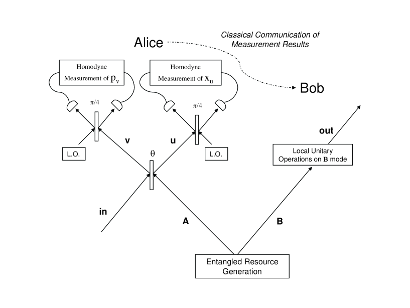
Figure 2.1: The Experimental Setup for Continuous Variable Teleportation. Alice mixes input mode $in$ with mode $A$ of the entangled state that is used as a teleportation resource by means of the beam-splitter ”$\theta$”. An homodyne measurement of nonlocal, commuting $x_{u}$ , $p_{v}$ quadratures is performed, ”collapsing” the joint state of modes $A$ and $in$ into an EPR state and transferring the initial state of mode $in$ onto mode $B$; save for a phase-space displacement corresponding to the actual values of the quadratures measured. This displacement is corrected for by Bob on receiving a communication of the measurement results from Alice.

Initially, the joint system of input and resource is in a state given by the Wigner function

$$W_{AB}(\alpha_{A};\,\alpha_{B})\;W_{in}(\alpha_{in})$$ (2.1)

The ”$\theta$” beam-splitter, with transmission coefficient $\cos(\theta)$ (fig. (2.1)) mixes the modes incoming modes $A$ and $in$, producing the outcoming modes $u$ and $v$ corresponding to nonlocal phase-space variables $\alpha_{u}$ and $\alpha_{v}$. The state of the system after the beam-splitter operation is given by

$$W_{AB}(\alpha_{A}(\alpha_{u},\alpha_{v}),\>\alpha_{B})\;W_{in}(\alpha_{in}(\alpha_{u},\alpha_{v}))$$ (2.2)

where variables $\alpha_{A}(\alpha_{u},\alpha_{v})\>,\;\alpha_{in}(\alpha_{u},\alpha_{v})$ are given by the inverse of the transformation in eq. (1.27) (see also eq. (1.26)).

On such a entangled state of $A$ and $in$ modes homodyne measurements of the nonlocal, commuting quadratures $x_{u}$ and $p_{v}$ are performed; thus a Bell observable measurement is realized. The state of part $B$ of the system after a projective measurement with results $x^{\prime}_{u}$ and $p^{\prime}_{v}$ is represented by the partial trace over $A$ and $in$ (see eq. (1.53) of the Wigner function of the system (eq. (2.2) and the Wigner function $W_{x^{\prime}_{u},p^{\prime}_{v}}$ (eq. (1.59)) of the respective element  of the Bell measurement;

$$W_{measured}(\alpha_{B}\,;\,x^{\prime}_{u},p^{\prime}_{v})=\pi^{-2}\>\int d^{2}\alpha_{in}\,d^{2}\alpha_{A}\;W_{AB}(\alpha_{A}(\alpha_{u},\alpha_{v}),\>\alpha_{B})\;W_{in}(\alpha_{in}(\alpha_{u},\alpha_{v}))$$

$$\times\,\mathcal{C}\>\delta(\cos(\theta)x_{in}\,-\,\sin(\theta)x_{A}\,-\,x^{\prime}_{u})\;\delta(\sin(\theta)p_{in}\,+\,\cos(\theta)p_{A}\,-\,p^{\prime}_{v})$$ (2.3)

$W_{measured}(\alpha_{B};\>x^{\prime}_{u},p^{\prime}_{v})$ in eq. (2.3) is not a normalized Wigner function (as is the case in eqs. (1.33) and (1.66)). It is the product of the probability $\mathrm{P}(x^{\prime}_{u},p^{\prime}_{v})$ of a measurement result $x^{\prime}_{u}\,,\,p^{\prime}_{v}$ and the Wigner function of the state of the $B$ part of the system after a measurement giving such a result; given by the conditional pseudo-probability $W_{measured}(\alpha_{B}\,|\>x^{\prime}_{u},p^{\prime}_{v})$. The probability can be obtained from eq. (2.3) by tracing out the $B$ mode;

$$\mathrm{P}(x^{\prime}_{u},p^{\prime}_{v})\,=\,\pi^{-1}\>\int d^{2}\alpha_{B}\>W_{measured}(\alpha_{B};\>x^{\prime}_{u},p^{\prime}_{v})$$ (2.4)

Perform the integral over $\alpha_{A}$ in eq. (2.3), yielding a convolution integral of the resource and the input states;

$$W_{measured}(\alpha_{B};\>x^{\prime}_{u},p^{\prime}_{v})\,=\,\frac{\pi^{-2}\mathcal{C}}{|\sin(\theta)|\>|\cos(\theta)|}\>\int d^{2}\alpha_{in}\>W_{in}(\alpha_{in})$$

$$\times W_{AB}(x_{in}\cot(\theta)\,-\,x^{\prime}_{u}\csc(\theta)\,+\,i\,\left(p_{v}\sec(\theta)\,-\,p_{in}\tan(\theta)\right);\>\alpha_{B})$$ (2.5)

Up to this point, we have not discussed the operations that Bob must perform on $B$ mode. Only to see clearly what these might be, we will consider an ideal resource, the EPR state of Wigner function

$$W_{AB}(\alpha_{A};\>\alpha_{B})=\,2\mathcal{C}\>\delta(x_{A}\,-\,x_{B})\;\delta(p_{A}\,+\,p_{B})$$ (2.6)

Substituting this resource in eq. (2.5 and integrating yields the resulting, un-normalized Wigner function;

$$\frac{2\,\pi^{-2}\,\mathcal{C}^{2}}{|\sin(\theta)|\>|\cos(\theta)|}W_{in}(x_{B}\tan(\theta)\,+\,x^{\prime}_{u}\sec(\theta)\,+\,i\,(p_{B}\cot(\theta)\,+\,p^{\prime}_{(}v)\csc(\theta)))$$ (2.7)

where the probability of obtaining the arbitrary result $x^{\prime}_{u},p^{\prime}_{v}$ of measurement is easily seen to be the vanishing constant $2\,\mathcal{C}^{2}\,\pi^{-2}\;(|\sin(\theta)|\>|\cos(\theta)|)^{-1}$.

To recover the input state at his end, Bob must perform two unitary operations on the $B$ mode; one of them after knowing the results of the measurement, communicated by Alice via a classical channel. Namely,

• A displacement in phase-space of $(x^{\prime}_{u}\sec(\theta)\,+\,i\,p^{\prime}_{v}\csc(\theta))$. For homodyne measurement apparatus with gain coefficients $0\,<\,g_{x}\,\leq\,1$ and $0\,<\,g_{p}\,\leq\,1$ for $x_{u}$ and $p_{v}$, respectively; this displacement will be $(g_{x}x^{\prime}_{u}\sec(\theta)+i\,g_{p}p^{\prime}_{v}\csc(\theta))$. Thus the operation is $\widehat{D}((g_{x}x^{\prime}_{u}\sec(\theta)+i\,g_{p}p^{\prime}_{v}\csc(\theta)))$.

• A transformation $x_{B}\,+\,i\,p_{B}\longrightarrow ax_{B}\,+\,i\,a^{-1}p_{B}$, with $a\equiv\,\cot(\theta)$. Therefore, is is a squeezing operation $\widehat{S}(r)$, where $e^{-r}\,=\,\cot(\theta)$. Obviously, $\cot(\theta)$ is part of the description of the beam-splitter inside our experimental setup and can be known beforehand by Alice and Bob.

The complete unitary operation applied by Bob would be given by the operator

$$\widehat{U}_{B}= \,\widehat{S}_{B}(-\ln(\cot(\theta)))\;\widehat{D}_{B}((x^{\prime}_{u}\sec(\theta)\,+\,i\,p^{\prime}_{v}\csc(\theta)))$$

$$= \,\widehat{D}_{B}((x^{\prime}_{u}\csc(\theta)\,+\,i\,p^{\prime}_{v}\sec(\theta)))\;\widehat{S}_{B}(-\ln(\cot(\theta)))$$ (2.8)

The squeezing operation performed by Bob can be made unnecessary. Consider a teleportation resource of the form

$$W_{AB}(\alpha_{A};\>\alpha_{B})=\,\mathcal{C}\,\delta(x_{A}\tan(\theta)\,-\,x_{B})\delta(p_{A}\cot(\theta)\,+\,p_{B})$$ (2.9)

instead of that of eq. (2.6). This would give the end result

$$\frac{\pi^{-2}\,\mathcal{C}^{2}}{|\sin(\theta)|\>|\cos(\theta)|}W_{in}(x_{B}\,+\,x^{\prime}_{u}\sec(\theta)\,+\,i\,(p_{B}\,+\,p^{\prime}_{(}v)\csc(\theta)))$$ (2.10)

thus, in this case, Bob must perform only the displacement above described to recover the input state and realize teleportation.

Note that a squeezing transformation $x_{A}+i\,p_{A}\longrightarrow\cot(\theta)x_{A}+i\,\tan(\theta)p_{A}$ (identical to Bob’s squeezing ”correction”) on mode $A$ of the resource in eq. (2.6) would result in the resource of eq. (2.9). A displacement of $(x^{\prime}_{u}\csc(\theta)+i\,p^{\prime}_{v}\sec(\theta))$ on mode $A$ of the resource in eq. (2.9) would yield the EPR state $W_{x^{\prime}_{u},p^{\prime}_{v}}$, identical to the state of the $A$ and $in$ modes after the Bell measurement with results $x^{\prime}_{u},p^{\prime}_{v}$. The unitary transformations on mode $A$ described above; transforming the EPR state in eq. (2.6) into the EPR state $W_{x^{\prime}_{u},p^{\prime}_{v}}$ of eq. (1.59) are identical to those applied by Bob to mode $B$ to realize teleportation (in eq. (2.8).

We have just shown that teleportation using an asymmetric beam-splitter of angle $\theta$ together with the simplest maximally entangled resource (eq. (2.6), will result in added squeezing on the output state. That squeezing will have to be corrected by the application of the inverse squeezing transformation. Previously applying this inverse transformation to mode $A$ of the resource will eliminate the need for such a correction by Bob.

The use of an asymmetric beam-splitter for mixing the $A$ and $in$ modes would be desirable only if the teleportation protocol were intended to produce an squeezed output. The effect of having an asymmetric beam-splitter in the experimental setup can be mimicked by appropriate local transformations on the resource state.

In order to simplify exposition, and assuming that we have no further use for additional squeezing of the output state we will take the beam-splitter ”$\theta$” to be symmetric ($\theta=\pi/4$) and without a phase. The use of a symmetric beam-splitter with a phase would only rotate in phase-space the displacement to be performed by Bob.

Using a symmetric beam-splitter, and after Bob’s correction (the displacement in eq. (2.8)) we have for the output state of the system (see eq. (2.5));

$$W_{out}(\alpha_{B};\>x^{\prime}_{u},p^{\prime}_{v})=\,2\,\pi^{-2}\,\mathcal{C}\>\int d^{2}\alpha_{in}\>W_{in}(\alpha_{in})$$

$$\times\,W_{AB}(x_{in}\,-\,2^{1\!/2}\,x^{\prime}_{u}\,+\,i\,(2^{1\!/2}\,p^{\prime}_{v}\,-\,p_{in});\>\alpha_{B}\,-\,(2^{1\!/2}\,g_{x}\,x^{\prime}_{u}\,+\,i\,2^{1\!/2}\,g_{p}\,p^{\prime}_{v}))$$ (2.11)

This output of teleportation is un-normalized, and so far dependent on the outcome $x^{\prime}_{u},p^{\prime}_{v}$ of the Bell measurement. It is the product of a probability for such an outcome and a conditional Wigner function (see eq. (2.3). Given

• the fundamental randomness of the results of quantum measurement, particularly Bell measurement of $x^{\prime}_{u},p^{\prime}_{v}$.

• that teleportation is, in principle performed in an absence of any knowledge (by Alice and Bob) of the input state; thus in the absence of any knowledge, even statistic, of measurement results.

• that teleportation is performed in an automatic manner by Alice and Bob, without change to the experimental setup due to the knowledge of particular set of measurement results.

• that for a realistic fidelity of teleportation, it is necessary to consider all the random outcomes of measurement, modulated by their probability; a fidelity coefficient depending on a single random result is not acceptable because it cannot be repeated reliably.

• that a conditional output state, on a random result is not an acceptable answer for a teleportation output, as it comes about randomly.

it becomes evident that a final output state that is acceptable is given by a mixture of conditional states (see eq. (2.3)) with the probability of measurement in eq. (2.4). Therefore, integration over $x^{\prime}_{u}$ and $p^{\prime}_{v}$ of eq. (2.11) will yield a normalized Wigner function that is an ensemble of conditional output states corresponding to individual measurement results,

$$W_{out}(\alpha_{B})= \,\mathcal{C}^{-1}\>\int dx^{\prime}_{u}\,dp^{\prime}_{v}\;W_{out}(\alpha_{B};\>x^{\prime}_{u},p^{\prime}_{v})$$

$$= \,2\,\pi^{-2}\,\int d^{2}\alpha_{in}\;W_{in}(\alpha_{in})$$

$$\times\,\int dx^{\prime}_{u}\,dp^{\prime}_{v} \;W_{AB}(x_{in}\,-\,2^{1\!/2}\,x^{\prime}_{u}\,+\,i\,(2^{1\!/2}\,p^{\prime}_{v}\,-\,p_{in});\>\alpha_{B}\,-\,(g_{x}\,2^{1\!/2}\,x^{\prime}_{u}\,+\,i\,g_{p}\,2^{1\!/2}\,p^{\prime}_{v}))$$ (2.12)

The Wigner function $W_{out}(\alpha_{B})$ is the outcome of the convolution of the Wigner function of the input $W_{in}$ and a bipartite (on $in$ and $B$ modes) Wigner function given by

$$K(\alpha_{in};\alpha_{B})=2\,\pi^{-1}\int dx^{\prime}_{u}\,dp^{\prime}_{v}\;W_{AB}(x_{in}\,-\,2^{1\!/2}\,x^{\prime}_{u}\,+\,i\,(2^{1\!/2}\,p^{\prime}_{v}\,-\,p_{in});\>\alpha_{B}\,-\,(g_{x}\,2^{1\!/2}\,x^{\prime}_{u}\,+\,i\,g_{p}\,2^{1\!/2}\,p^{\prime}_{v}))$$ (2.13)

named the teleportation kernel in the literature [69, 73]. It is easily seen that the kernel is the Wigner function of an ensemble (with constant, flat probability) of Transfer Operators [26, 74] (one for each value of $x^{\prime}_{u}\,,\,p^{\prime}_{v}$), having the Wigner function

$$W_{AB}(x_{in}\,-\,2^{1\!/2}\,x^{\prime}_{u}\,+\,i\,(2^{1\!/2}\,p^{\prime}_{v}\,-\,p_{in});\>\alpha_{B}\,-\,(g_{x}\,2^{1\!/2}\,x^{\prime}_{u}\,+\,i\,g_{p}\,2^{1\!/2}\,p^{\prime}_{v}))$$ (2.14)

Let the characteristic function $\chi_{out}(\xi_{B})$ be the Fourier transform of $W_{out}(\alpha_{B})$ (see eq. (1.48);

$$\chi_{out}(\xi_{B})=\,2\,\pi^{-3}\>\int d^{2}\alpha_{B}\,\int d^{2}\alpha_{in}\,\int dx^{\prime}_{u}\,dp^{\prime}_{v}\>e^{2i(x_{B}z_{B}\,-\,p_{B}w_{B})}$$

$$\times W_{in}(\alpha_{in})\;W_{AB}(x_{in}\,-\,2^{1\!/2}\,x^{\prime}_{u}\,+\,i\,(2^{1\!/2}\,p^{\prime}_{v}\,-\,p_{in});\>\alpha_{B}-(g_{x}\,2^{1\!/2}\,x^{\prime}_{u}\,+\,i\,g_{p}\,2^{1\!/2}\,p^{\prime}_{v}))$$ (2.15)

Making the substitution $x^{\prime\prime}_{u}\equiv\,2^{1\!/2}\,x^{\prime}_{u}$, $p^{\prime\prime}_{v}\equiv\,2^{1\!/2}\,p^{\prime}_{v}$, and multiplying the integrand in eq. (2.15) by $e^{\pm\,2\,i\,(g_{x}\,z_{B}\,x^{\prime\prime}_{u}\,-\,g_{p}\,w_{B}\,p^{\prime\prime}_{v})}$ we obtain

$$\chi_{out}(\xi_{B})= \,\pi^{-1}\,\int d^{2}\alpha_{in}\;W_{in}(\alpha_{in})\;\pi^{-1}\,\int dx^{\prime\prime}_{u}\,dp^{\prime\prime}_{v}\>e^{2\,i\,(z_{B}\,g_{x}\,x^{\prime\prime}_{u}\,-\,w_{B}\,g_{p}\,p^{\prime\prime}_{v})}$$

$$\times\,\pi^{-1}\,\int d^{2}\alpha_{B}\>e^{2\,i\,(z_{B}\,(x_{B}\,-\,g_{x}\,x^{\prime\prime}_{u})\,-\,w_{B}\,(p_{B}\,-\,g_{p}\,p^{\prime\prime}_{v}))}$$

$$\times\,W_{AB}(x_{in}\,-\,x^{\prime\prime}_{u}\,+\,i\,(p^{\prime\prime}_{v}\,-\,p_{in});\>\alpha_{B}\,-\,(g_{x}\,x^{\prime\prime}_{u}+\,i\,g_{p}\,p^{\prime\prime}_{v}))$$ (2.16)

This is an explicit Fourier transformation over the $\alpha_{B}$, $x^{\prime\prime}_{u}\,+\,i\,p^{\prime\prime}_{v}$ variables; as well as a convolution over $\alpha_{in}$. Therefore, the characteristic function of the output state is straightforward to calculate:

$$\chi_{out}(\xi_{B})=\,\chi_{AB}(g_{p}\,w_{B}\,-\,i\,g_{x}\,z_{B};\>\xi_{B})\;\chi_{in}(g_{p}\,w_{B}\,+\,i\,g_{x}\,z_{B})$$ (2.17)

A result equivalent to that obtained in ref. [75] for a symmetric beam-splitter using the transfer operator formalism.

Keeping the beam-splitter asymmetric, and having Bob perform the squeezing operation described in eq. (2.8) will result in output state

$$\chi_{out}(\xi_{B})=\,\chi_{AB}(g_{p}\,w_{B}\,-\,i\,g_{x}\,z_{B}\,;\>\tan(\theta)\,w_{B}\,+\,i\,\cot(\theta)\,z_{B})\;\chi_{in}(g_{p}\,\tan(\theta)\,w_{B}\,+\,i\,g_{x}\,\cot(\theta)\,z_{B})$$ (2.18)

2.2 Teleportation in the language of characteristic functions

The derivation of the CV teleportation output made in the previous section will now be repeated in the characteristic function representation and will be shown to be much simpler. The experimental setup for teleportation is illustrated, as before, in fig. (2.1). Let the initial state of the joint system $A,B,in$ be described by their characteristic functions

$$\chi_{AB}(\xi_{A};\>\xi_{B})\;\chi_{in}(\xi_{in})$$ (2.19)

There is a (symmetric) beam-splitter transformation from this initial state into the modes $u$ and $v$ and their associated quadratures, which, it can be seen easily (see eq. (1.48)), transforms the conjugate phase-space variables $\xi_{in},\xi_{A}$ in a similar manner to eq. (1.27) to $\xi_{u}\,\,xi_{v}$. We will consider the EPR state’s characteristic function (eq. (1.60)) in terms of the variables $\xi_{in},\xi_{A}$. And realize the partial trace, or projection into the POVM element (for results $x^{\prime}_{u},p^{\prime}_{v}$) thus,

$$\chi_{measured}(\xi_{B};\>x^{\prime}_{u},p^{\prime}_{v})=\, \pi^{-2}\,\int\,d^{2}\xi_{in}\,d^{2}\xi_{A}\;\chi_{AB}(\xi_{A};\>\xi_{B})\;\chi_{in}(\xi_{in})\;\chi_{x^{\prime}_{u},p^{\prime}_{v}}(-\xi_{in}\,,\,-\xi_{A})$$

$$= \pi^{-2}\,\int\,d^{2}\xi_{in}\,d^{2}\xi_{A}\;\chi_{AB}(\xi_{A};\>\xi_{B})\;\chi_{in}(\xi_{in})$$

$$\times\,2\,\mathcal{C}\,\delta(w_{in}\,-\,w_{A})\>\delta(z_{in}\,+\,z_{A})\>e^{-2\,i\,\left(z_{in}\,2^{1\!/2}\,x^{\prime}_{u}\,-\,w_{in}\,2^{1\!/2}\,p^{\prime}_{v}\right)}$$ (2.20)

This characteristic function is, like its Wigner function equivalent in eq. (2.3), un-normalized. It is the product of the probability of measurement $\mathrm{P}(x^{\prime}_{u},p^{\prime}_{v})$ of a result $x^{\prime}_{u},p^{\prime}_{v}$ and the conditional characteristic function of the system $\chi_{measured}(\xi_{B}|x^{\prime}_{u},p^{\prime}_{v})$, on the aforementioned results. Tracing out the $B$ mode in eq. (2.21) will give us the probability of measurement;

$$\mathrm{P}(x^{\prime}_{u},p^{\prime}_{v})=\,\pi^{-1}\,\int d^{2}\xi_{B}\;\chi_{measured}(\xi_{B};\>x^{\prime}_{u}\,,\,p^{\prime}_{v})$$ (2.21)

With the purpose of having a look into Bob’s part in the teleportation protocol, we will consider the resource to be in a simple EPR state of the form

$$\chi_{AB}(\xi_{A};\>\xi_{B})=\,2\,\mathcal{C}\>\delta(w_{A}-w_{B})\>\delta(z_{A}+z_{B})$$ (2.22)

Performing integration of eq. (2.20) with the aforementioned resource yields

$$\chi_{measured}(\xi_{B};\>x^{\prime}_{u},p^{\prime}_{v})=4\,\pi^{-2}\,\mathcal{C}^{2}\,\chi_{in}(\xi_{B})\,e^{\,2\,i\,\left(w_{B}\,2^{1\!/2}\,p^{\prime}_{v}\,-\,z_{B}\,2^{1\!/2}\,x^{\prime}_{u}\right)}$$ (2.23)

which is a product of the characteristic function of the input state $\chi_{in}$ (in mode $B$), with an additional phase-space displacement of $-2^{1\!/2}x^{\prime}_{u}\,-\,i2^{1\!/2}p^{\prime}_{v}$; and a constant probability for every single result of measurement of $4\pi^{-2}\mathcal{C}^{2}$. This result is consistent with that of eq. (2.7) (for $\theta=\pi/4$). Thus, Bob must perform that which, to his knowledge (given the non-unit gain of the apparatus) is the opposite displacement operation, $\widehat{D}_{B}(g_{x}\,2^{1\!/2}\,x^{\prime}_{u}\,+\,i\,g_{p}\,2^{1\!/2}p^{\prime}_{v})$ to recover the input state;

$$\chi_{out}(\xi_{B};\>x^{\prime}_{u},p^{\prime}_{v})\,=\,e^{-2\,i\,\left(w_{B}\,g_{p}\,2^{1\!/2}p^{\prime}_{v}\,-\,z_{B}\,g_{x}\,2^{1\!/2}x^{\prime}_{u}\right)}\;\chi_{measured}(\xi_{B};\>x^{\prime}_{u},p^{\prime}_{v})$$ (2.24)

For the same reasons and on the same considerations exposed in the previous section; an ouput state conditional on a random measurement result is not acceptable, while an ensemble of conditional states with adequate probability is an acceptable output state. Therefore, integrate eq. (2.24) over $x^{\prime}_{u}$ and $p^{\prime}_{v}$ to obtain the normalized, ensemble state

$$\chi_{out}(\xi_{B})= \,\mathcal{C}^{-1}\,\int dx^{\prime}_{u}\,dp^{\prime}_{v}\;\chi_{out}(\xi_{B};\>x^{\prime}_{u},p^{\prime}_{v})$$

$$= \,2\,\pi^{-2}\,\int dx^{\prime}_{u}\,dp^{\prime}_{v}\>\int\,d^{2}\xi_{in}\>d^{2}\xi_{A}\;e^{-\,2\,i\,\left(w_{B}\,g_{p}\,2^{1\!/2}p^{\prime}_{v}\,-\,z_{B}\,g_{x}\,2^{1\!/2}x^{\prime}_{u}\right)}$$

$$\times\;\delta(w_{in}\,-\,w_{A})\>\delta(z_{in}\,+\,z_{A})\>e^{-\,2\,i\,\left(z_{in}\,2^{1\!/2}x^{\prime}_{u}\,-\,w_{in}\,2^{1\!/2}p^{\prime}_{v}\right)}$$

$$\times\;\chi_{AB}(\xi_{A};\>\xi_{B})\;\chi_{in}(\xi_{in})$$ (2.25)

The integration of eq. (2.25) is entirely straightforward, giving the output state

$$\chi_{out}(\xi_{B})=\,\chi_{in}(g_{p}w_{B}\,+\,i\,g_{x}z_{B})\;\chi_{AB}(g_{p}w_{B}\,-\,ig_{x}z_{B};\>\xi_{B})$$ (2.26)

which is identical to that obtained in eq. (2.17), after a much shorter and more elegant calculation.

The formalism just outlined is general for any combination of resource and input states and gives a very simple expression for the output of Quantum Teleportation in CV. It is possible to use resources that are mixed states, reflecting the results of a conditional operation performed during the preparation of said resource. Or to construct input states that are mixtures of the states (or likely superpositions thereof) used to encode qudits in quantum information processing with adequate probabilities; thus constructing the general input ensemble of a quantum CV channel of teleportation, for which the fidelity can be calculated.

A basic analysis of eq. (2.26) shows that obtaining a result other than a random, ”classical” guess depends on having a high measurement gain ($g_{x},g_{p}\approx 1$) and on having a resource characteristic function $\chi_{AB}(g_{p}w_{B}\,-\,ig_{x}z_{B};\xi_{B})$ that is nearly constant. This last condition is fulfilled by states approximating the EPR state of eq. (2.22). For example two-mode squeezed vacuums at high squeezing $r$; or other states showing great similarity with a two-mode squeezed vacuum at high squeezing.

2.3 Teleportation: a projective measurement onto a mixed state

We have produced a simple formalism for the representation of the elementary transformations and projective measurements performed in CV teleportation and produced a compact expression for the characteristic function of a general output state, for all resource states. It is conceivable that the first and most obvious change in the teleportation protocol involves the EPR state onto which we project to represent an homodyne measurement (see section 1.4 and eq. (2.20)).

The first choice if we are interested in the introduction of ”imperfect” homodyne measurements would be a suitable mixture of EPR states. What would a mixture imply? That we are still doing an homodyne measurement of the variables $x_{u},p_{v}$ and projecting onto an EPR state. We do not know which state precisely, even if the apparatus for homodyne detection returns a result $x^{\prime}_{u},p^{\prime}_{v}$. If the apparatus is imprecise (not damaged or lacking calibration) the distribution of outcomes will be centered on the values returned. We can define such a projecting state as the mixture

$$\hat{\rho}_{mix}= \,\pi^{-1}\,\int\,dx_{-}\,dp_{+}\;\mathrm{P}(x_{-},p_{+};\>x^{\prime}_{u},p^{\prime}_{v})\;\hat{\rho}_{x_{-}\,,\,p_{+}}$$ (2.27)

$$\chi_{mix}(\xi_{in},\xi_{A})= \,\pi^{-1}\,\int\,dx_{-}\,dp_{+}\;\mathrm{P}(x_{-},p_{+};\>x^{\prime}_{u},p^{\prime}_{v})\;\chi_{x_{-},p_{+}}(\xi_{in},\xi_{A})$$ (2.28)

where $\chi_{x_{-},p_{+}}(\xi_{in},\xi_{A})$ is the EPR state of eq. (1.60) ($\Theta=\pi/4$) for eigenvalues $x_{-}$ and $p_{+}$. The probability distribution $\mathrm{P}(x_{-},p_{+};x^{\prime}_{u},p^{\prime}_{v})$ is required to fulfill the following conditions if the state in eq. (2.28) is to represent an imprecise measuring apparatus;

$$\pi^{-1}\,\int\,dx_{-}\,dp_{+}\;\mathrm{P}(x_{-},p_{+};\>x^{\prime}_{u},p^{\prime}_{v})=1$$

$$\mathrm{P}(x_{-},p_{+};\>x^{\prime}_{u},p^{\prime}_{v})=\mathrm{P}(x_{-}-x^{\prime}_{u}\,,\,p_{+}-p^{\prime}_{v})$$

$$\bar{x}_{-}=\,x^{\prime}_{u}\;\;\;\;\bar{p}_{+}=\,p^{\prime}_{v}$$ (2.29)

namely to be normalized and ”centered” around $x^{\prime}_{u}\,,\,p^{\prime}_{v}$.

The mixture of EPR states of eq. (2.28) for such a probability distribution is given by

$$\chi_{mix}(\xi_{in},\xi_{A})=\; \pi^{-1}\,\int\,dx_{-}\,dp_{+}\mathrm{P}(x_{-}-x^{\prime}_{u},p_{+}-p^{\prime}_{v})\,2\,\mathcal{C}\,e^{2i\left(z_{in}2^{1\!/2}x_{-}\,-\,w_{in}2^{1\!/2}p_{+}\right)}$$

$$\times\delta(z_{in}+z_{A})\delta(w_{in}-w_{A})$$ (2.30)

Let us define the Fourier transform of $\mathrm{P}(x,p)$, the characteristic function

$$\widetilde{\mathrm{P}}(w,z)=\,\pi^{-1}\>\int\,dx\,dp\;e^{2\,i\,\left(z\,x\,-\,w\,p\right)}\;\mathrm{P}(x,p)$$ (2.31)

Using the definition of eq. (2.31), we can write the characteristic function in eq. (2.30) in a more elegant manner;

$$\chi_{mix}(\xi_{in},\xi_{A})=\,\widetilde{\mathrm{P}}(2^{1\!/2}w_{in}\,,\,2^{1\!/2}z_{in})\;2\,\mathcal{C}\>\delta(z_{in}\,+\,z_{A})\>\delta(w_{in}\,-\,w_{A})\;e^{2\,i\,\left(z_{in}\,2^{1\!/2}x^{\prime}_{u}\,-\,w_{in}\,2^{1\!/2}p^{\prime}_{v}\right)}$$ (2.32)

To study the corrections to be made by Bob we substitute the mixture state eq. (2.32) into eq. (2.20) in place of the EPR state $\chi_{x^{\prime}_{u},p^{\prime}_{v}}$; and take the resource to be an EPR state (eq. (2.22)), yielding an output state

$$\chi_{measured,mix}(\xi_{B};\>x^{\prime}_{u},p^{\prime}_{v})\,=\,4\,\pi^{-2}\,\mathcal{C}^{2}\;\widetilde{\mathrm{P}}(-2^{1\!/2}w_{B}\,,\,-\,2^{1\!/2}z_{B})\;\chi_{in}(\xi_{B})\;e^{\,2\,i\,\left(w_{B}\,2^{1\!/2}p^{\prime}_{v}\,-\,z_{B}\,2^{1\!/2}x^{\prime}_{u}\right)}$$ (2.33)

We have the product of the constant probability for a given result equal to that in eq. (2.23); of the characteristic function $\widetilde{\mathrm{P}}$; and of the characteristic function of the input state, displaced in phase-space by $-(x^{\prime}_{u}2^{1\!/2}\,+\,ip^{\prime}_{v}2^{1\!/2})$. Bob will try to correct for this displacement by applying at his end the displacement $\widehat{D}_{B}(g_{x}\,2^{1\!/2}\,x^{\prime}_{u}\,+\,i\,g_{p}\,2^{1\!/2}p^{\prime}_{v})$ on $B$ mode. Again, the apparatus is assumed to have non-unit gains $g_{x}$ and $g_{p}$.

Proceeding in the same manner of section 2.2; performing the displacement just described on the characteristic function in eq. (2.24), and taking the final output state to be an ensemble of outcomes corresponding to measurement results $x^{\prime}_{u},p^{\prime}_{v}$ (see eq. (2.25)) will result in the final output state

$$\chi_{out,mix}(\xi_{B})=\,\widetilde{\mathrm{P}}(-2^{1\!/2}g_{p}\,w_{B}\,,\,-2^{1\!/2}g_{x}\,z_{B})\;\chi_{in}(g_{p}\,w_{B}\,+\,i\,g_{x}\,z_{B})\;\chi_{AB}(g_{p}\,w_{B}\,-\,i\,g_{x}\,z_{B};\>\xi_{B})$$ (2.34)

This is the same characteristic function of the output state in eq. (2.26) multiplied by the characteristic function $\widetilde{\mathrm{P}}(-2^{1\!/2}g_{p}\,w_{B}\,,\,-2^{1\!/2}g_{x}\,z_{B})$.

The output state of the previous section is thus ”smeared” in phase-space. This is easily seen in the Wigner functions’ language; as this product of characteristic functions is the Fourier transform of the convolution integral between the probability $\mathrm{P}$ and the pseudo-probability $W_{in}$. For example, a nearly constant characteristic function $\widetilde{\mathrm{P}}$ (the Fourier transform of a sharply peaked function $\mathrm{P}(x,p)\sim\,\delta(x)\>\delta(p)$) will yield an output state in eq. (2.34) approximating the ideal output state of eq. (2.26).

The natural choice for a probability distribution $\mathrm{P}(x,p)$ intended to represent a measurement apparatus producing outcomes (as far as regards the projection caused by the measurement) with a random deviation from the ”real”, mean values $x^{\prime}_{u},p^{\prime}_{v}$ is the Gaussian distribution;

$$\mathrm{P}(x,p)= \;e^{r+s}\,e^{-e^{2r}x^{2}\,-\,e^{2s}p^{2}}$$ (2.35)

$$\widetilde{\mathrm{P}}(w,z)= \;e^{-e^{-2r}z^{2}\,-\,e^{-2s}w^{2}}$$ (2.36)

producing a multiplying factor in eq. (2.34) of

$$e^{-\left(\,2\,e^{-2r}\,g_{x}^{2}\,z_{B}^{2}\,\right)}\;e^{-\left(\,2\,e^{-2s}\,\,g_{p}^{2}\,w_{B}^{2}\,\right)}$$ (2.37)

Reducing the measurement gains $g_{x},g_{p}$ might improve the output state, for input characteristic functions $\chi_{in}(g_{p}w_{B}\,+\,ig_{x}z_{B})$ that become constant at a much slower rate than a Gaussian distribution when the variables $g_{x}z_{B}\,,\,g_{p}w_{B}$ grow small, or for input characteristic functions with a wide support, the Fourier transforms of narrow Wigner functions.

2.4 Mixed teleportation resources: ”superimposed” over noisy environments

We have calculated the characteristic function for a mixture of EPR states (eq. (2.32) in section 2.3. In doing so, we have stated some properties of the mixture probability (eq. (2.29)) that ensure consistency with our hypothesis of an imperfect measurement and greatly simplify the form of the output of teleportation when the projective measurement is done onto this mixture (eq. (2.34).

In this section; we will derive the characteristic function of a teleportation resource that is a mixture of pure states in phase-space. Our first purpose is to obtain the teleportation output when such a mixture is used as a resource. Our second purpose is to obtain within our formalism a well-known result for normally ordered phase-space pseudo-distributions. Namely the result of superimposing a state of the radiation field over another, preexisting state having a $P(\alpha)$ function [35, 38, 76]. It is generally understood that a given (pure) resource state will propagate in a spatial volume or be prepared ideally within the environment given by the pure vacuum $|0\,,\,0\,\rangle$ state. In ref. [38] it is spoken of the switching on/off of two sources in order; which is equivalent to preparing one state over another (or letting one state propagate over the same spatial volume of the) state we have deemed to be an initial environment. The superimposition  we will consider in this section consists in preparing (or letting propagate) a two-mode teleportation resource state when the initial environment state is different from the vacuum and has a $P(\alpha)$ function. We will use environment states that are generally considered ”noise” for our purposes; for example, separable, two-mode thermal states.

Given the pure state $\hat{\rho}_{AB}$, let us define the phase-space mixture of states in an similar manner to that of eq. (2.27);

$$\hat{\rho}^{(Mix)}_{AB}=\,\pi^{-2}\,\int\,d^{2}\alpha_{a}\,\,d^{2}\alpha_{b}\;\mathrm{P}_{A}(x_{a}\,,\,p_{a})\>\mathrm{P}_{B}(x_{b}\,,\,p_{b})\;\hat{\rho}_{AB,\alpha_{a};\>\alpha_{b}}$$ (2.38)

where $\mathrm{P}_{A}$ and $\mathrm{P}_{B}$ are probability distributions that fulfill the conditions set forth in eq. (2.29). The density operator

$$\hat{\rho}_{AB,\alpha_{a};\>\alpha_{b}}=\,\widehat{D}^{{\dagger}}_{B}(\alpha_{b})\;\widehat{D}^{{\dagger}}_{A}(\alpha_{a})\;\hat{\rho}_{AB}\;\widehat{D}_{A}(\alpha_{a})\;\widehat{D}_{B}(\alpha_{b})$$ (2.39)

is that of an ideal, pure state resource; displaced in phase-space by $\alpha_{a}$ and $\alpha_{b}$. Thus, the density operator of eq. (2.38) is equivalent to that for two superimposed modes in ref. [38]. Note that the density operator for any phase-space mixture; for example the mixed EPR state (eq. (2.27) is of a similar form, as phase-space displacements transform one EPR state into another EPR state.

The characteristic function of eq. (2.38) is thus given by

$$\chi^{(Mix)}_{AB}(\xi_{A};\>\xi_{B})=\, \pi^{-2}\,\int\,d^{2}\alpha_{a}\,d^{2}\alpha_{b}\;\mathrm{P}_{A}(x_{a}\,,\,p_{a})\;\mathrm{P}_{B}(x_{b}\,,\,p_{b})$$

$$\times\,e^{\,2\,i\,\left(z_{A}x_{a}\,-\,w_{A}p_{a}\right)}e^{\,2\,i\,\left(z_{B}x_{b}\,-\,w_{B}p_{b}\right)}\;\chi_{AB}(\xi_{A};\;\xi_{B})$$ (2.40)

where displacement operations correspond to phase factors in the characteristic function. Define the characteristic functions $\widetilde{\mathrm{P}}_{A}$ and $\widetilde{\mathrm{P}}_{B}$ as the Fourier transforms of $\mathrm{P}_{A}$ and $\mathrm{P}_{B}$ (see eq. (2.31)). The characteristic function in eq. (2.40) will have the factorized form

$$\chi^{(Mix)}_{AB}(\xi_{A};\>\xi_{B})=\,\widetilde{\mathrm{P}}_{A}(w_{A}\,,\,z_{A})\;\widetilde{\mathrm{P}}_{B}(w_{B}\,,\,z_{B})\;\chi_{AB}(\xi_{A};\>\xi_{B})$$ (2.41)

The characteristic function of eq. (2.41) can be made equivalent to the superimposition of the resource state $\hat{\rho}_{AB}$ over initial states in modes $A$ and $B$. If the Wigner functions for such initial states can be substituted for the probability distributions $\mathrm{P}_{A}$ and $\mathrm{P}_{B}$ in the mixture. This can be done only for Wigner functions fulfilling certain conditions; being finite, nonnegative and normalized. In other words, for Wigner functions that are genuine probability distributions. In refs. [38, 35, 76], the equivalent condition is set forth that the initial states possess a $P(\alpha)$ function representation.

The Wigner function that is the Fourier transform of eq. (2.41) is given by

$$W^{(Mix)}_{AB}(\alpha_{A};\>\alpha_{B})=\,\pi^{-2}\,\int\,d^{2}\alpha_{a}\,d^{2}\alpha_{b}\;W_{AB}(\alpha_{A}\,-\,\alpha_{a};\>\alpha_{B}\,-\,\alpha_{b})\;\mathrm{P}_{A}(x_{a},p_{a})\\ ;\mathrm{P}_{B}(x_{b},p_{b})$$ (2.42)

which is a convolution integral of the Wigner functions of the states. This relation is equivalent to that of the $P(\alpha)$ functions for ”superposed” excitations in ref. [38].

The general mixed states that we have used as substitutes for the EPR states in projective measurement in section 2.3 can be thought of as superimpositions of a pure state on a ”noisy” initial environment. The probability distribution in eq. (2.27) is nonlocal; therefore it must be the nonnegative Wigner function of a nonlocal state. General, Gaussian entangled states, having nonnegative Wigner functions would be the first choice. This kind of superimposition can be interesting; but it falls outside of the scope of our work. We consider entangled states ”pure” resources to be prepared; not noisy environments to ”prepare over”.

We have chosen separate probabilities $\mathrm{P}_{A}$ and $\mathrm{P}_{B}$ instead of a joint probability in eq. (2.38; it is our purpose to represent preparation of a resource over ”noisy” separable states and study the changes wrought by this new preparation on separability and teleportation fidelity, with respect to a pure state prepared over a two-mode vacuum.

Thermal states on modes $A$ and $B$ constitute a noisy initial state over which the pure resource state can be prepared, resulting in a mixed resource state. Thermal states [38] fulfill the requisite of having a positive Wigner function and having a $P(\alpha)$ representation. They are prime candidates for the representation of the simplest noisy environments. A single-mode thermal field of mean photon-number $n_{Th}$ has a density matrix in the Fock basis

$$\rho_{th}=\,\sum_{k}\;\frac{n_{th}^{k}}{(1+n_{th})^{k+1}}\;|\,k\,\rangle\>\langle\,k\,|$$ (2.43)

and a Gaussian [48, 38] Wigner function that is a genuine probability distribution. Which, along with its respective characteristic function, reads

$$W_{th}(\alpha)\, =\,n_{th}^{-1}\;e^{-n_{th}^{-2}|\alpha|^{2}}$$ (2.44)

$$\chi_{th}(\xi)\, =\;e^{-n_{th}^{2}|\xi|^{2}}$$ (2.45)

The characteristic functions of quantum states chosen to represent noise will appear as multiplicative factors in the output of teleportation. Substituting the resource of eq. (2.41) in eq. (2.26) yields the outcome

$$\chi_{out}(\xi_{B})=\,\chi_{in}(g_{p}w_{B}\,+\,i\,g_{x}z_{B})\;\chi_{AB}(g_{p}w_{B}\,-\,i\,g_{x}z_{B};\>\xi_{B})\widetilde{\mathrm{P}}_{A}(g_{p}w_{B}\,,\,-g_{x}z_{B})\>\widetilde{\mathrm{P}}_{B}(w_{B}\,,\,z_{B})$$ (2.46)

This output has in common with eq. (2.34) the presence of a multiplicative factor; though of a different character. The mixture in that case is that of the ”homodyne” projective measurement as ”induced” by an imprecise apparatus. In this case the factor corresponds to a phase-space mixture that is the result of preparation of the resource in a noisy environment.

2.5 Losses and noise admission in the projective measurement

In the previous sections we have used the characteristic functions language to produce an expression for teleportation outcome. We have introduced modifications to the protocol that imply, in our view, imprecisions in the homodyne measurement. We have formulated a ”noisy”, mixed resource state.

A modification to the teleportation procedure is the next step. We will modify the teleportation protocol by the introduction of fictitious elements, with the initial purpose of modelling a realistic, lossy and noisy homodyne measurement. Setups introducing fictitious elements to homodyne detection were originally developed and adapted to the study of non ideal, ”realistic” homodyne detection of single mode quadratures in the $Q(\alpha)$ function representation [34]; and later independently developed for non ideal teleportation in a coherent state representation [77].

The realistic homodyne measurement will be realized by the addition of two beam-splitters of rather high transmittances $\cos^{2}(\phi)$ and $\cos^{2}(\varphi)$, where $\phi\,\approx\,\varphi\,\approx\,1$; and two ”external” modes that will be mixed by these beam-splitters with the nonlocal modes (those originally to be measure: $u$ and $v$ in fig. (2.1)) before the actual process of homodyne measurement takes place. These beam-splitters will also deduct a small loss of intensity to the original nonlocal modes.

The setup for this lossy, noisy homodyne measurement is illustrated in fig. (2.2) (see the left half of fig. (2.1) for a comparison). The beam-splitters ”$\phi$” and ”$\varphi$” and modes $d_{0}$ and $e_{0}$ are the new elements in the homodyne setup. For the external modes a choice can be made of thermal states, vacuum states, or general one-mode Gaussian states including the aforementioned as special cases.

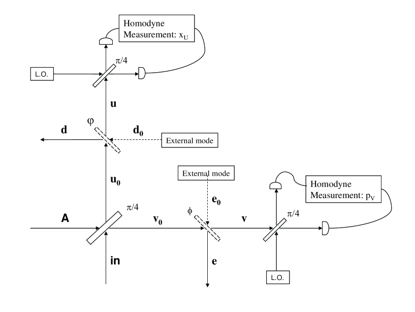
Figure 2.2: The Experimental Setup for Realistic Homodyne Measurement in CV Teleportation. The external modes $d_{0}$ and $e_{0}$ are mixed with the nonlocal modes $u_{0}$ and $v_{0}$ by the ”$\varphi$” and ”$\phi$” beam splitters. The resulting $u$ and $v$ modes undergo homodyne measurement and ”projection” onto an EPR state.

The teleportation procedure will (as always) consist in the performance of a projective measurement of the quadratures $x_{u},p_{v}$. These are derived from the initial ”$0$” quadratures by the beam-splitter transformations for the modes illustrated in fig. (2.2),

$$\begin{pmatrix}\alpha_{u_{0}}\\ \alpha_{v_{0}}\end{pmatrix}= \begin{pmatrix}2^{-1\!/2}&-2^{-1\!/2}\\ 2^{-1\!/2}&2^{-1\!/2}\end{pmatrix}\begin{pmatrix}\alpha_{in}\\ \alpha_{A}\end{pmatrix}$$

$$\begin{pmatrix}\alpha_{u}\\ \alpha_{d}\end{pmatrix}= \begin{pmatrix}\cos(\varphi)&-\sin(\varphi)\\ \sin(\varphi)&\cos(\varphi)\end{pmatrix}\begin{pmatrix}\alpha_{u_{0}}\\ \alpha_{d_{0}}\end{pmatrix}$$

$$\begin{pmatrix}\alpha_{v}\\ \alpha_{e}\end{pmatrix}= \begin{pmatrix}\cos(\phi)&-\sin(\phi)\\ \sin(\phi)&\cos(\phi)\end{pmatrix}\begin{pmatrix}\alpha_{v_{0}}\\ \alpha_{e_{0}}\end{pmatrix}$$ (2.47)

With these transformations at hand, it is easy to write the Wigner function of the appropriate EPR state for homodyne measurement (see eq. (1.59)) having eigenvalues $x^{\prime}_{u}$ and $p^{\prime}_{v}$;

$$W_{x^{\prime}_{u}\,,\,p^{\prime}_{v}}(\alpha_{u_{0}},\alpha_{d_{0}};\>\alpha_{v_{0}},\alpha_{e_{0}})\,= \,\mathcal{C}\;\delta\left(\cos(\varphi)\,x_{u_{0}}\,-\,\sin(\varphi)\,x_{d_{0}}\,-\,x^{\prime}_{u}\right)$$

$$\times\,\delta\left(\cos(\phi)\,p_{v_{0}}\,-\,\sin(\phi)\,p_{e_{0}}\,-\,p^{\prime}_{v}\right)$$ (2.48)

The characteristic function for the EPR state is obtained in a straightforward manner by Fourier transformation of the above expression, and is given by

$$\chi_{x^{\prime}_{u}\,,\,p^{\prime}_{v}}(\xi_{u_{0}},\xi_{d_{0}};\>\xi_{v_{0}},\xi_{e_{0}})\,= \,\pi^{2}\,\mathcal{C}\;\delta(w_{d_{0}})\;\delta(z_{v_{0}})\;\delta(w_{u_{0}})\delta(z_{e_{0}})\;\delta\left(\sin(\varphi)\,z_{u_{0}}\,+\,\cos(\varphi)\,z_{d_{0}}\right)$$

$$\times\,\delta\left(\sin(\phi)\,w_{v_{0}}\,+\,\cos(\phi)\,w_{e_{0}}\right)e^{-\,2\,i\,\left(z_{d_{0}}\,x^{\prime}_{u}\,\csc(\varphi)\,-\,w_{e_{0}}\,p^{\prime}_{v}\,\csc(\phi)\right)}$$ (2.49)

The state of the joint system $AB,in$ to be measured after the first, symmetric ($\pi/4$) beam-splitter reads

$$\chi_{in}(2^{-1\!/2}\xi_{u_{0}}\,+\,2^{-1\!/2}\xi_{v_{0}})\;\chi_{AB}(2^{-1\!/2}\xi_{v_{0}}\,-\,2^{-1\!/2}\xi_{u_{0}};\>\xi_{B})\;\chi_{ext.\>u}(\xi_{d_{0}})\;\chi_{ext.\>v}(\xi_{e_{0}})$$ (2.50)

where $\chi_{ext.\>u}$ and $\chi_{ext.\>v}$ are the characteristic functions of the two external modes $d_{0}$ and $e_{0}$, respectively.

We follow the teleportation protocol as described in section 2.2 for the physical system in eq. (2.50); using for the projective measurement the EPR state of eq. (2.49). As before, we have Bob perform a displacement of $\widehat{D}_{B}(x^{\prime}_{u}2^{1\!/2}\,+\,ip^{\prime}_{v}2^{1\!/2})$ to correct the output state; only with the gains $g_{x}=g_{p}=1$; for the procedure we are performing already includes losses in intensity and is intended to model a lossy measurement. The output state will be, as before, an ensemble of all possible measurement outcomes. Thus,

$$\chi_{out,n}(\xi_{B})= \,\mathcal{C}^{-1}\,\int\,dx^{\prime}_{u}\,dp^{\prime}_{v}\,e^{\,2\,i\,\left(z_{B}\,2^{1\!/2}\,x^{\prime}_{u}\,-\,w_{B}\,2^{1\!/2}\,p^{\prime}_{v}\right)}$$

$$\times\,\pi^{-4}\,\int\,d^{2}\xi_{u_{0}}\,d^{2}\xi_{v_{0}}\,d^{2}\xi_{d_{0}}\,d^{2}\xi_{e_{0}}\;\chi_{in}(2^{-1\!/2}\xi_{u_{0}}\,+\,2^{-1\!/2}\xi_{v_{0}})$$

$$\times\,\chi_{AB}(2^{-1\!/2}\xi_{v_{0}}\,-\,2^{-1\!/2}\xi_{u_{0}};\>\xi_{B})\;\chi_{ext.\>u}(\xi_{d_{0}})\;\chi_{ext.\>v}(\xi_{e_{0}})$$

$$\times\;\chi_{x^{\prime}_{u}\,,\,p^{\prime}_{v}}(\xi_{u_{0}},\xi_{d_{0}};\>\xi_{v_{0}},\xi_{e_{0}})$$ (2.51)

After some (entirely straightforward) integration of the above expression, we obtain the output state

$$\chi_{out,n}(\xi_{B})\,= \,\chi_{in}(\cos(\phi)\,w_{B}\,+\,i\,\cos(\varphi)\,z_{B})\;\chi_{AB}(\cos(\phi)\,w_{B}\,-\,i\,\cos(\varphi)\,z_{B};\>\xi_{B})$$

$$\times\,\chi_{ext.\>u}(i\,2^{1\!/2}\sin(\varphi)\,z_{B})\;\chi_{ext.\>v}(2^{1\!/2}\sin(\phi)\,w_{B})$$ (2.52)

The first obvious trait of this state is the multiplication by the characteristic functions of the external modes. These have arguments that are scaled by the (small) factors $\sin(\varphi)$ and $\sin(\phi)$, while the characteristic functions of input and resource are scaled by factors (close to $1$) $\cos(\varphi)$ and $\cos(\phi)$ which are the transmission coefficients for the beam-splitters ”$\phi$” and ”$\varphi$”, respectively. For small angles $\phi$ and $\varphi$, eq. (2.52) approximates eq. (2.26) for gains given as $g_{x}=\,\cos(\varphi)$ and $g_{p}=\,\cos(\phi)$. In the limit case $\phi=\varphi=0$ eq. (2.52) equals eq. (2.26), as the characteristic functions of the external modes with argument $0$ are constant.

In sections 2.3 and 2.4 we have multiplying characteristic functions of probability distributions (which can be also Wigner functions) as multiplying factors in teleportation output states. But there are two main differences. First, it is not required by the formalism we have used that $\chi_{ext.\>u}$ and $\chi_{ext.\>v}$ be the Fourier transforms of nonnegative Wigner functions. Second and most important, the multiplying factors in the arguments of said characteristic functions are $\sin(\varphi)$ and $\sin(\phi)$: not the gains; but rather the complementary quantities of those which may be considered measurement gains ($\cos(\varphi)$ and $\cos(\phi)$). Only in the case where the Wigner functions of the external modes are positive and $\phi=\varphi=\pi/4$ (or $g_{x}=g_{p}=2^{-1/2}$) are the two cases entirely equivalent. These two differences illustrate the ”lossy” nature of the teleportation protocol outlined here, as compared with the merely ”noisy” protocols.

There is an obvious choice of external modes’ states to represent losses and added noise in a teleportation setup [34, 77]. It is the general one-mode Gaussian vacuum states, which may be squeezed and of non-minimum uncertainty (thermal). Such thermal states have a characteristic function

$$\chi_{Th(n,s)}(\xi)=e^{-\,\bar{n}^{2}(e^{-2s}z^{2}+e^{2s}w^{2})}$$ (2.53)

for an average number of photons $n$ and a squeezing parameter $s$ (squeezing applied on $\hat{x}$ quadrature). Given similarly squeezed thermal states with the same average number of photons for both the external modes, the multiplying factor in eq. (2.52) will be

$$e^{\,-\,2\bar{n}^{2}\,e^{-2s}\,\sin(\varphi)^{2}\,z_{B}^{2}}\;e^{\,-\,2\,\bar{n}^{2}\,e^{2s}\,\sin(\phi)^{2}\,w_{B}^{2}}$$ (2.54)

As explained before, the main difference with the examples of Gaussian mixtures in the previous sections is that this ”smearing factor” will tend to become constant as the measurement gain goes to $1$.

2.6 Teleportation fidelity with characteristic functions

We have adopted the definition of fidelity proposed in ref. [39]. In the characteristic function representation this is equal to eq. (1.71). This is the scalar product, or the trace of the product of density operators, for the input and output states. Let us take, for simplicity of exposition, the output state we have derived in eq. (2.26) (for a maximum gain $g_{x}=g_{p}=1$) and insert it in eq. (1.71);

$$\mathcal{F}=\,\pi^{-1}\,\int\,d^{2}\xi_{B}\;\chi_{in}(\xi_{B})\;\chi_{in}(-\xi_{B})\>\chi_{AB}(-\xi_{B}^{*};\>-\xi_{B})$$ (2.55)

A summary analysis might be made of this expression and of its integrand. We have inside the integrand that $\chi_{in}(\xi_{B})\>\chi_{in}(-\xi_{B})=|\chi_{in}(\xi_{B})|^{2}$. This quantity is a real, even, nonnegative characteristic function itself, corresponding to the square of the density operator $\hat{\rho}_{in}^{2}$ (see eqs. (1.52) and 1.51)). Its trace integral over $\xi_{B}$ is equal to the purity of the input state. In eq. (2.55) it is multiplied by the characteristic function of the resource state $\chi_{AB}$. When the resource state approximates an EPR state, its characteristic function becomes nearly constant with a value of $1$ (which is not square integrable). The result is ideal teleportation with maximal fidelity: $1$ for pure input states and the value of the purity for mixed input states.

Given that the fidelity is real, positive and bounded from above, we remark that $\chi_{AB}(\pm\xi_{B}^{*};\pm\xi_{B})$ has to be bounded and must have an imaginary part that is odd or $0$. Its real part must be even and positive (in the sense that an application is positive).

The fidelity in eq. (2.55) is quadratic in the input state and linear in the resource state. The fidelities corresponding to the output states derived in sections 2.2, 2.3 and 2.5 share these two features; even though there are additional multiplying factors.

One very simple conclusion to be drawn from the linearity of the teleportation output and of the fidelity with respect to the resource state is that we need only calculate the fidelity of teleportation for pure resource states, as the fidelity for a simple mixture of resource states comes about trivially. Given a mixture of pure resource states $|\,\psi_{i}\,\rangle_{AB}$, and given the characteristic function’s linearity with respect to the density operator (see eq. (1.54)), we have that

$$\hat{\rho}_{AB}= \,\sum_{i}\>\mathrm{P}_{i}\;|\,\psi_{i}\,\rangle_{AB}\;\langle\,\psi_{i}\,|_{AB}$$

$$\chi_{AB}(\xi_{A};\>\xi_{B})= \,\sum_{i}\>\mathrm{P}_{i}\;\chi_{\psi_{i}\,,\,AB}(\xi_{A};\>\xi_{B})$$ (2.56)

where $\chi_{\psi_{i}\,,\,AB}$ are the characteristic functions of the pure states $|\,\psi_{i}\,\rangle_{AB}$.

Given the linearity of the fidelity (eq. (2.55)) with respect to the above characteristic function; it follows that the fidelity of teleportation using this mixed resource state is simply the weighted average of the fidelities $\mathcal{F}_{i}$ resulting from the use of the pure resource states singly as teleportation resources;

$$\mathcal{F}=\,\sum_{i}\>\mathrm{P}_{i}\;\mathcal{F}_{i}$$ (2.57)

Therefore, we need only concern ourselves with pure resource states, at least as regards discrete mixtures of resources. These discrete mixtures appear whenever one considers conditional preparation procedures for resources; such as photon subtraction and addition for two-mode squeezed Gaussian states, which involve measurements.

The fidelity of teleportation is quadratic with respect to the input state. For an input state that is a mixture of other (pure) input states with characteristic functions $\chi_{in,j}(\xi_{in})$, we have

$$\chi_{in}(\xi_{in})=\sum_{j}\mathrm{P}_{j}\;\chi_{in,j}(\xi_{in})$$ (2.58)

The fidelity of teleportation in eq. (2.55 for the above mixture is given by

$$\mathcal{F}=\,\sum_{j,k}\>\mathrm{P}_{j}\>\mathrm{P}_{k}\;\pi^{-1}\,\int\,d^{2}\xi_{B}\;\chi_{in,j}(\xi_{B})\;\chi_{in,k}(-\xi_{B})\;\chi_{AB}(-\xi_{B}^{*};\>-\xi_{B})$$ (2.59)

which is rather complicated. The integrals summed in eq. (2.59) are traces of the input pure state ”$i$” with the output state resulting from the teleportation ”$j$”. The integrals are not (individually) bona fide teleportation fidelities; save for the case where $i=j$, but must sum to a teleportation fidelity that is bounded. The summation over the integrals is not equivalent to the average of fidelities in eq. (2.58. Even in the case of a near-ideal resource; eq. (2.59) includes terms that are the casual overlap of the components of the input mixture, and the (nearly) perfect transcriptions resulting from teleportation. This can be seen as a limitation in the concept of fidelity we have adopted.

If we consider the mixture above described as the ensemble of likely (one qudit) inputs of a quantum teleportation channel for a CV [68] or hybrid quantum computation scheme [29]; we can count on the likely inputs for the channel to be far away from each other as regards scalar product: nearly orthogonal or orthogonal, so as to be easily distinguishable by measurement apparatus even under noisy conditions. In that case, and for a good enough teleportation resource, we can consider eq. (2.59) to include mainly the contribution from the $i=j$ traces (bona fide teleportation fidelities) that sum to a weighted average fidelity.

Chapter 3 Teleportation with degaussified, squeezed Fock and squeezed Bell-like resources

In the previous chapter we introduced a formalism for the study of teleportation in CV based on the Wigner characteristic function representations of quantum states. The expression for the output state derived for the ideal CV protocol (section 2.2) is general for any combination of teleportation resource and input having Wigner and Wigner characteristic functions.

The objective of the investigation of teleportation resources is to produce feasible teleportation schemes that improve the teleportation fidelity for the input states most likely to be used in CV quantum computation [68, 20] or in hybrid schemes that use CV states for communication [29, 31]. The original protocol [33] was developed for Gaussian two-mode squeezed states, and these will be used as the benchmark from which it is desirable to improve output state fidelity, for a fixed squeezing parameter $r$. The parameter $r$ assumes the meaning of indicator of technological capability in the preparation of resources.

An initial analysis of non-Gaussian resources can begin with the class of ”degaussified” two-mode squeezed states that have been shown to produce an improvement in the teleportation fidelity with respect to Gaussian states of both a comparable covariance matrix and similar squeezing parameter $r$ [21, 22, 23, 3].

”Degaussification”  is the production of a non-Gaussian state of the radiation field by conditional photon subtraction (addition) on an initially Gaussian state. This procedure is both performed and verified by appropriate single-photon measurements. The ”simulation” of the conditional measurement and the use of the subsequent mixtures of degaussified and Gaussian resources has been done  in refs. [21, 23, 3]. Within the characteristic function representation, we have shown (see section 2.6) that the use of any such mixture as a resource gives results for fidelity that can be trivially derived from the results for pure state resources.

We have found useful for the search of improvements in teleportation fidelity to formulate classes of resource states that encompass the largest possible categories of Gaussian, degaussified or simply non-Gaussian states. These generalizing classes of resources are by definition non-Gaussian. They are necessarily superpositions of the ”special case” resources or involve additional unitary transformations on such states; moreover, they reduce to the special case states for particular choices of the superposition and unitary transformation parameters. These same parameters can be arbitrarily chosen, allowing us to sculpt teleportation resources; even to optimize the resource for maximal fidelity of teleportation of a given input state. A further and related advantage lies in the ability to compare optimal resources with special case resource states for which preparation strategies have been devised or experimentally tested; having been proposed in previous work for CV quantum information resources.

In this chapter, we will first introduce the non-Gaussian resources and inputs used throughout the chapter, in the characteristic function representation. We will then study the fidelity in the teleportation of selected pure input states; using photon-subtracted and photon-added squeezed states, two-mode squeezed Gaussian states, two-mode squeezed Fock states; and as implied before, a class of states that includes the aforementioned resource states as special cases. These we have named the squeezed Bell-like states in previous work [24]; general superpositions of the two-mode, Gaussian squeezed vacuum state and the two-mode squeezed Fock state of number $1,1$, which is non-Gaussian. For the squeezed Bell-like resource states, we have calculated an optimal fidelity (with respect to the superposition parameters) for each of the selected input states [24] and compared this optimal fidelity with the (smaller) fidelities obtained for the resources mentioned above.

The optimal squeezed Bell-like states and the ”special case” resources are also studied and compared as to entanglement, non-Gaussian character and affinity with Gaussian states; with the purpose of establishing the characteristics of a non-Gaussian state that better correlate with teleportation fidelity. The parameters for comparison are the von Neumann entropy [78]; a non-Gaussianity measure [79], and a two-mode squeezed vacuum ”affinity” measure devised for non-Gaussian teleportation resources [24].

3.1 Resources and inputs: state vectors and characteristic functions

In this section, we will introduce the two-mode non-Gaussian states that are the object of our study as resources for CV teleportation in this chapter.

3.1.1 Squeezed Fock states

The two-mode squeezed Fock state is prepared by the performance of a two-mode squeezing operation on a CV system that is in a (separable) two-mode Fock state. The state vector for this wholly non-Gaussian state is given by,

$$|\zeta\,;\>m_{A}\,,\,m_{B}\,\rangle\,=\,\widehat{S}_{AB}(\zeta)\;|\,m_{A}\,,\,m_{B}\,\rangle_{AB}$$ (3.1)

where $\widehat{S}_{AB}(\zeta)$ is the two-mode squeezing operator of eq. (1.41); with the separable state vector $|\,m_{A}\,,\,m_{B}\,\rangle_{12}\equiv|\,m_{A}\,\rangle_{A}\otimes|\,m_{B}\,\rangle_{B}$ being the two-mode Fock state.

The two-mode squeezed vacuum state $\widehat{S}_{AB}(\zeta)\;|\,\zeta\,;\,0,0\,\rangle$ and the two-mode squeezed Fock state $\widehat{S}_{AB}(\zeta)|\,\zeta\,;\,1\,1\,\rangle$ are special instances of this class of states. This last state will be referred to as two-mode squeezed Fock state throughout the chapter.

The calculation of the characteristic function for the two-mode squeezed Fock state is straightforward, given that it is pure state; hence it’s characteristic function is given by eq. (1.55). Thus

$$\chi_{SN}^{(1,1)}(\xi_{A};\xi_{B})=\;\langle 1,1|\,\widehat{S}^{{\dagger}}_{AB}(\zeta)\>\widehat{D}_{A}(\xi_{A})\>\widehat{D}_{B}(\xi_{B})\>{S}_{AB}(\zeta)|\,1,1\rangle$$ (3.2)

Recall the Bogoliubov transformation effected by the unitary two-mode squeezing operator on the displacement operators (see eq. (1.45)) and the expression for the matrix element of the displacement operator in the Fock basis [46];

$$\langle\,m\,|\>\widehat{D}(\xi)|\,n\,\rangle\,=\,\left(\frac{n!}{m!}\right)^{1/2}\xi^{m-n}\>e^{-\frac{1}{2}|\,\xi\,|^{2}}\>L_{n}^{(m-n)}(|\,\xi\,|^{2})$$ (3.3)

where $L_{n}^{(m-n)}$ is the associated Laguerre polynomial [80].

Given the above relations, the characteristic function for the state $|\,\zeta\,;\>1\,,1\rangle$ is easily seen to be

$$\chi_{SN}^{(1,1)}(\,\xi_{A};\>\xi_{B}\,)=\,e^{-1\ ,/\,2\>\left(|\,\xi^{\prime}_{A}\,|^{2}\,+\,|\,\xi^{\prime}_{B}\,|^{2}\right)}\;\left(1-|\,\xi^{\prime}_{A}\,|^{2})(1-|\,\xi^{\prime}_{B}\,|^{2}\right)$$ (3.4)

where the variables $\xi^{\prime}_{A}$ and $\xi^{\prime}_{B}$ are related to the variables $\xi_{A}$ and $\xi_{B}$ via the Bogoliubov transformation described in eq. (1.46) for the displacement operator arguments.

3.1.2 Degaussified resource states

The degaussified resource states are generated by photon subtraction (or addition) to each of the modes $A$ and $B$ of a two-mode squeezed Gaussian state. Although the photon subtraction (addition) procedure is conditional in most experimental setups, it will be assumed here that it has been successfully performed and verified, obtaining a pure resource state. Thus, the photon subtracted (added) states have the state vectors

$$|m_{A}^{(-)}\,,\,m_{B}^{(-)}\,;\>\zeta\,\rangle\,= \,\mathcal{N}_{AB}^{\,(-)}\;a_{A}^{m_{A}}\;a_{B}^{m_{B}}\;\widehat{S}_{AB}(\zeta)\;|\,0\,,\,0\,\rangle_{AB}$$ (3.5)

$$|m_{A}^{(+)}\,,m_{B}^{(+)}\,;\zeta\rangle\,= \,\mathcal{N}_{AB}^{\,(+)}\;a_{A}^{{\dagger}\;m_{A}}\;a_{B}^{{\dagger}\;m_{B}}\;\widehat{S}_{AB}(\zeta)\;|\,0\,,\,0\,\rangle_{AB}$$ (3.6)

where $\mathcal{N}_{AB}^{\,\pm}$ are normalization constants specific to each state vector. Henceforth, and in keeping with the proposals for the experimental generation of these states [7, 8, 9, 10, 11], we will restrict our analysis to the case where $m_{A}=m_{B}=1$; to the single-photon subtracted (added) states.

To easily calculate the normalization constants and the respective characteristic functions, and to put the degaussified states in a proper perspective with respect to the other resources studied in this chapter; we write the states described in eqs. (3.5) and (3.6), taking into account the transformation that results from the application of the two-mode squeezing operator on the annihilation and creation operators (see eq. (1.44)),

$$|1^{(-)}\,,\,1^{(-)};\>\zeta\,\rangle= \,\mathcal{N}\;e^{i\phi}\widehat{S}_{AB}(\zeta)\;\left(-|\,0\,,\,0\,\rangle_{AB}\>+\>e^{i\phi}\,\tanh(r)\,|\,1\,,\,1\,\rangle_{AB}\right)$$ (3.7)

$$|1^{(+)}\,,\,1^{(+)};\>\zeta\,\rangle= \,\mathcal{N}\;e^{-i\phi}\widehat{S}_{AB}(\zeta)\;\left(-\tanh(r)\,|\,0\,,\,0\,\rangle_{AB}\>+\>e^{i\phi}\,|\,1\,,\,1\,\rangle_{AB}\right)$$ (3.8)

where $\mathcal{N}=\,[\,1\,+\,\tanh^{2}(r)\,]^{-1/2}$ is the normalization constant for both desgaussified states. Thus, degaussified resources are shown to be superpositions of the two-mode squeezed vacuum and the two-mode squeezed Fock state.

However, eqs. (3.7) and (3.8) substantially differ in the exchange of the hyperbolic coefficients for the superposition, and in the character of the state for vanishing squeezing. Even if both states become separable for $r=0$, the photon-added squeezed state reduces to the non-Gaussian two-mode Fock state; while the photon-subtracted squeezed state becomes the Gaussian the two-mode vacuum.

The calculation of the characteristic functions for these degaussified resources makes use of the same relations (eqs. (1.45), (1.46), (3.2) and (3.3)) used in the derivation of the characteristic function of the two-mode squeezed Fock state (eq. (3.4)). Recall that the degaussified resources are superpositions of two-mode squeezed Fock states (eqs. (3.7) and (3.8)). The density matrices have the form

$$\hat{\rho} =\,|\,K_{0}\,|^{2}|\,\zeta\,,\,0\,,\,0\,\rangle\>\langle\,\zeta\,,\,0\,,\,0\,|\>+\>|\,K_{1}\,|^{2}|\,\zeta\,,\,1\,,\,1\,\rangle\>\langle\,\zeta\,,\,1\,,\,1|$$

$$+\,K_{0}^{*}K_{1}\,|\,\zeta\,,\,1\,,\,1\,\rangle\>\langle\,\zeta\,,\,0\,,\,0\,|\>+\>K_{1}^{*}K_{0}\,|\,\zeta\,,\,0\,,\,0\,\rangle\>\langle\,\zeta\,,\,1\,,\,1\,|$$ (3.9)

with the factors $K_{0,1}$ taking the appropriate values for photon-subtracted or added states. Terms in eq. (3.9) correspond to (Fock basis) matrix elements of the displacement operator (see eq. (3.3)) in the calculation of the characteristic function. The characteristic functions of the photon-subtracted and photon-added two-mode squeezed states are thus given by

$$\chi_{PSS}^{\,(1,1)}\,(\xi_{A};\>\xi_{B})= \,{\mathcal{N}}^{\,2}\;e^{-1/2\>\left(|\,\xi^{\prime}_{A}\,|^{2}\,+\,|\,\xi^{\prime}_{B}\,|^{2}\right)}\;\{1\,-\,2\tanh(r)\>\mathrm{Re}[e^{-\,i\,\phi}\xi^{\prime}_{A}\,\xi^{\prime}_{B}]$$

$$+\,\tanh^{2}(r)\>(1-|\,\xi^{\prime}_{A}\,|^{2})\>(1-|\,\xi^{\prime}_{B}\,|^{2})\}$$ (3.10)

$$\chi_{PAS}^{\,(1,1)}(\xi_{A};\>\xi_{B})= \,{\mathcal{N}}^{\,2}\;e^{-1/2\>\left(|\,\xi^{\prime}_{A}\,|^{2}\,+\,|\,\xi^{\prime}_{B}\,|^{2}\right)}\;\{\tanh^{2}(r)\,-\,2\tanh(r)\>\mathrm{Re}[e^{-\,i\,\phi}\xi^{\prime}_{A}\,\xi^{\prime}_{B}]$$

$$+\,(1-|\,\xi^{\prime}_{A}\,|^{2})\>(1-|\,\xi^{\prime}_{B}\,|^{2})\}$$ (3.11)

where the relation of the variables $\xi^{\prime}_{A}$ and $\xi^{\prime}_{B}$ to the variables $\xi_{A}$ and $\xi_{B}$ is described by the Bogoliubov transformation of eq. (1.46) for the displacement operator arguments.

Comparing eq. (1.58) with eqs. (3.4), (3.10), and (3.11); we see that the polynomial terms that define the non-Gaussian character of the state are always multiplied by a Gaussian factor equal to the two-mode squeezed state characteristic function of eq. (1.58).

Lastly; it is worth remarking that the (non-Gaussian) two-mode photon-subtracted squeezed state can be defined as the first-order truncation of the (Gaussian) two-mode squeezed state. Let us consider the two-mode squeezed vacuum given by $|-\,2\,r\,\rangle\,=\,\widehat{S}_{AB}(-\,2\,r)\>|\,0\,,\,0\,\rangle_{AB}$. Recalling eq. (1.43); such a state can be written as

$$|-2\,r\,\rangle_{AB}\,= \,\widehat{S}_{AB}(-r)\;\widehat{S}_{AB}(-r)\;|\,0\,,\,0\,\rangle_{AB}$$

$$= \,\widehat{S}_{AB}(-r)\;\cosh^{-1}(r)\;\sum_{n=0}^{\infty}\>\left(\,\tanh(-r)\,\right)^{n}\>|\,n\,,\,n\,\rangle_{AB}$$ (3.12)

Truncating the series of eq. (3.12) beyond $n=1$ , we recover the photon-subtracted resource state (eq. (3.7)), with $\phi=\pi$; that is $|1^{(-)}\,,\,1^{(-)}\,;-r\,\rangle$. Moreover, this state coincides with that of the photon-subtracted state introduced in ref. [3] for the ideal case of a beam splitter with unity transmittance.

3.1.3 General non-Gaussian resources: Squeezed Bell-like states

In order to unify the study of the properties, of the teleportation performance, and of the experimental methods for the generation of the above mentioned resource states, we take into consideration a class of states that have been named the squeezed Bell-like states in previous work [24]. The state vector for the squeezed Bell-like state is given by

$$|\,\Psi\,\rangle_{SBell}\,=\,\widehat{S}_{AB}(\zeta)\>\left(\,\cos(\delta)\>|\,0\,,\,0\,\rangle_{AB}\;+\;e^{i\theta}\,\sin(\delta)\>|\,1\,,\,1\,\rangle_{AB}\right)$$ (3.13)

which is a superposition of the two-mode squeezed vacuum and the two-mode squeezed Fock state. The superposition coefficients are parameterized as $\cos(\delta)$ and $e^{i\,\theta}\sin(\delta)$, which is convenient as the free parameters $\delta$ and $\theta$ involved can be chosen arbitrarily; always having a normalized state vector.

The state in eq. (3.13) is two-mode squeezed. That it is Bell-like is apparent on inspection of eq. (1.64). For $r=0$ and $\delta=\pi/4$ the squeezed Bell-like state reduces to $|\,0\,,\,0\,\rangle_{AB}\,+\,e^{i\theta}|\,1\,,\,1\,\rangle_{AB}$; the Bell state for the two-dimensional Hilbert space spanned by Fock states $|\,0\,\rangle$ and $|\,1\,\rangle$; and the ideal resource for discrete variables quantum teleportation [81] of states belonging to that two-dimensional Hilbert space.

The squeezed Bell-like state will have as special cases all of the two-mode states that we consider as teleportation resources in this chapter; for appropriate values of the parameters $\delta$ and $\theta$, and will interpolate between these resources. Taking $\zeta=r$, we obtain a Gaussian resource for $\delta=0$, a squeezed Fock state for $\delta=\pi/2$, a photon-subtracted squeezed state for $\delta=\cos^{-1}(\mathcal{N}),\theta=\pi$ and a photon-added squeezed state for $\delta=\cos^{-1}(\mathcal{N}\tanh(r)),\theta=\pi$. The squeezed Bell-like state is inseparable for $r=0$, except for the aforementioned trivial choices of $\delta$ corresponding to squeezed vacuum and squeezed Fock state.

The advantage of interpolating between known resource states allows for an unifying study of their characteristics and of their performance as entangled resources for quantum information in CV. This advantage is compounded by the possibility of choosing the parameters $\delta$ and $\theta$ in an arbitrary manner, thus sculpting the entangled resource. For instance, given an input state, and an analytical expression for teleportation fidelity; this fidelity can be optimized with respect to the superposition parameters, for a fixed squeezing $r$. Even if squeezed Bell-like states are considered nothing more than theoretical constructs for the study of the teleportation fidelity for a wide variety of resources; it will always be possible to pick a suitable ”special case” to sculpt in an experimentally feasible manner so as to better approximate the optimal squeezed Bell-like state resource.

The squeezed Bell-like state is, like the degaussified states, a superposition of two-mode squeezed states. The density matrix for the squeezed Bell-like state is of the general form described in eq. (3.9). Calculating the characteristic function for this state involves repeating the procedure outlined above for the degaussified states; for a superposition with coefficients $\cos(\delta)$ and $e^{i\theta}\sin(\delta)$. The characteristic function of the squeezed Bell-like state reads

$$\chi_{SBell}(\xi_{A};\>\xi_{B})= \,e^{-1/2\,\left(|\,\xi^{\prime}_{A}\,|^{2}\,+\,|\,\xi^{\prime}_{B}\,|^{2}\right)}\>\{\cos^{2}(\delta)\>+\>2\cos(\delta)\,\sin(\delta)\,\mathrm{Re}[e^{\,i\,\theta}\xi^{\prime}_{A}\,\xi^{\prime}_{B}]$$

$$\,+\,\sin^{2}(\delta)\,(1\,-\,|\,\xi^{\prime}_{A}\,|^{2})\,(1\,-\,|\,\xi^{\prime}_{B}\,|^{2})\}$$ (3.14)

where, as before; $\xi^{\prime}_{A}$ and $\xi^{\prime}_{B}$ are related to $\xi_{A}$ and $\xi_{B}$ by the Bogoliubov transformation of eq. (1.46) for the displacement operator arguments.

3.1.4 Selected input states

The following single-mode input states have been considered for the study of teleportation with non-Gaussian resources, among a variety of Gaussian and non-Gaussian states that are likely inputs both in CV quantum computation and hybrid quantum computation: Coherent states; squeezed vacuum states; single-photon Fock states; squeezed single-photon Fock states and photon-added coherent states.

The characteristic functions for most of these one-mode states are straightforward to derive, and can be found in the literature, for example in refs. [47, 43].

For the coherent state $|\,\beta\,\rangle$ the characteristic function reads

$$\chi_{coh}(\xi_{in})\,=\,e^{-\frac{1}{2}|\,\xi_{in}\,|^{2}\,+\,2\,i\,\mathrm{Im}[\xi_{in}\beta^{*}]}$$ (3.15)

The one-mode squeezed vacuum state $|\,\varepsilon\,\rangle\,=\,\widehat{S}(\varepsilon)\>|\,0\,\rangle$ (where $(\varepsilon=e^{i\varphi}s)$) has a characteristic function given by

$$\chi_{sq}(\xi_{in})\,=\,e^{-\frac{1}{2}|\,\xi^{\prime}_{in}\,|^{2}}$$ (3.16)

where $\xi^{\prime}_{in}\,=\,\xi_{in}\cosh(s)\,+\,\xi_{in}^{*}e^{i\varphi}\sinh(s)$, a Bogoliubov transformation of variables.

The characteristic section for the squeezed Fock state $\widehat{S}(\varepsilon)\>|\,1\,\rangle$ can be calculated easily given eq. (3.3) and reads

$$\chi_{sqF}(\xi_{in})=\,e^{\,-\,\frac{1}{2}|\,\xi^{\prime}_{in}\,|^{2}}\>(1\,-\,|\,\xi^{\prime}_{in}\,|^{2})$$ (3.17)

with $\xi^{\prime}_{in}$ given by the above Bogoliubov transformation.

The characteristic function for the Fock state $|\,1\,\rangle_{in}$ is given by the trivial limit $s=0$ of eq. (3.17).

The (non-Gaussian) photon-added coherent state is prepared by the application of the creation operator $\hat{a}^{{\dagger}}$ to a coherent state;

$$(1\,+\,|\,\beta\,|^{2})^{-1/2}\>\hat{a}^{{\dagger}}\>|\,\beta\,\rangle$$ (3.18)

where, for $\beta=0$ eq. (3.18) reduces to the single-photon Fock state $|\,1\,\rangle$. The derivation of the characteristic function of the photon-added coherent state is; however, straightforward

$$\chi_{pac}(\xi_{in})\,=\,(1\,+\,|\,\beta\,|^{2})^{-1}\;e^{-\frac{1}{2}|\,\xi_{in}\,|^{2}\,+\,3\,i\,\mathrm{Im}[\xi_{in}\,\beta^{*}]}\;(1\,+\,|\,\beta\,|^{2}\,-\,|\,\xi_{in}\,|^{2}\,+\,2\,i\,\mathrm{Im}[\xi_{in}\,\beta^{*}])$$ (3.19)

3.2 Teleportation with degaussified and squeezed Fock resources

In this section, we compare the behavior of the teleportation fidelity for the input states described above; using as resources the two-mode squeezed Fock state (eq. (3.1)), and both the degaussified states (eqs. (3.7) and (3.8)).

We will assume ideal CV teleportation. Therefore, the output state characteristic function is given by eq. (2.26) (for $g_{x}=g_{p}=1$), and the teleportation fidelity is given by eq. (2.55). The fidelity is analytically computable for the the input states and entangled resources considered here; the integral in eq. (2.55) can be exactly calculated in terms of finite sums of averages over Gaussian distributions.

The fidelities of teleportation will be analyzed and compared for fixed and equal squeezing parameter $r$ for all resources. The performance of the Gaussian two-mode squeezed state will also be displayed for reference purposes, as it is generally considered a benchmark [39, 40]. This choice is made to compare the performance of Gaussian and chosen non-Gaussian resources, given the possession of the same technological means for their generation.

3.2.1 Teleportation of Gaussian input states

We begin our analysis with the teleportation of Gaussian input states. In fig. (3.1) we plot the fidelity of teleportation (see eq. (1.71)) having as inputs the coherent state $|\,\beta\,\rangle_{in}$ (Panel I), and the input squeezed vacuum state $|\,\beta\,\rangle_{in}$ (Panel II), for the resource states introduced above, with the exception of the squeezed Bell-like state. The phase of squeezing will be fixed as $\phi=\pi$ from now on; in keeping with the conventions established in the CV protocol outlined in chapter 2.

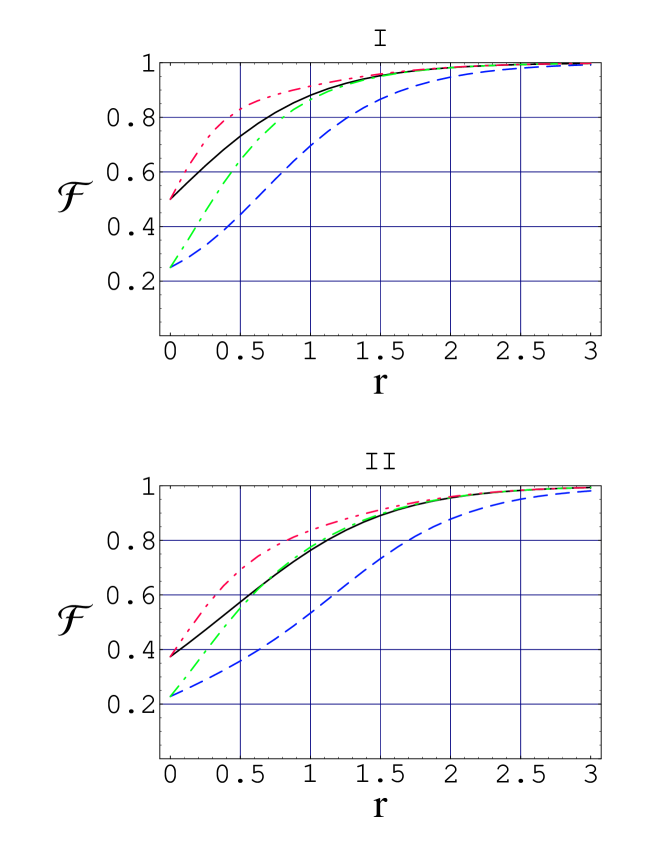
Figure 3.1: Fidelity of teleportation $\mathcal{F}$, as a function of the squeezing parameter $r$, with $\phi=\pi$, for input coherent state $|\beta\rangle$ (Panel I) and input squeezed vacuum state $|\,\varepsilon\,\rangle$ (Panel II). Comparison is given for different two-mode entangled resources: (a) squeezed state (full line); (b)  squeezed Fock state (dashed line); (c) photon-subtracted squeezed state (double-dotted, dashed line); (d) photon-added squeezed state (dot-dashed line). In plot I the value of $\beta$ is arbitrary. In plot II the squeezing parameter of the input state is fixed at $s=0.8$.

For both inputs in fig. (3.1); the choice of the photon-subtracted squeezed state (eq. (3.10)) as entangled resource is the most convenient one. It corresponds to the highest value of the fidelity $\mathcal{F}$ for any fixed value of the squeezing $r$ in the realistic range $[0,1]$. On the contrary, the choice of the squeezed Fock state (eq. (3.4)) as entangled resource is the least convenient, yielding the poorest performance; even when compared to the Gaussian squeezed resource. Finally, regarding the use of the photon-added squeezed state (eq. (3.11)) as entangled resource, it allows for a very modest improvement in the fidelity when compared to the Gaussian resource; and this only for a small interval of values around $r=1$. For smaller squeezing, its performance is poorer than that of the Gaussian resource.

The poor performance of the photon-added and two-mode squeezed Fock resources is not surprising for small squeezing parameters. The input in both cases is a Gaussian state; and both these resource states reduce to a two-mode Fock state for $r=0$. In Panel I of fig. (3.1) we see that the overlap of a coherent input state with a mixture of displaced  coherent states for classical teleportation is $0.5$, as expected from previous work on ”classical” teleportation [39, 40]. The overlap of the coherent input state with a mixture of randomly displaced one-photon Fock states is $0.25$. The probability for a given displaced element of the mixture is given by the probability of a result equal to the displacement; when the joint measurement of non-local quadratures of the $A$ and $in$ modes is performed (see subsection 1.4.2).

We must, finally, remark that the fidelity of teleportation is significantly higher for the coherent state input (Panel I,fig. (3.1)) than for the squeezed vacuum input (Panel II,fig. (3.1)), for all resources, for small $r$. This is due to the fact that the one-mode squeezing operation has an asymptotic limit $s\,\rightarrow\infty$ in which all squeezed states will approximate a quadrature eigenstate. In the case of quasi-classical teleportation, for small $r$, the randomly displaced, nearly uniform mixture in mode $B$ has little overlap with a squeezed input state; even for the moderate squeezing ($s=0.8$) chosen.

3.2.2 Teleportation of non-Gaussian input states

Let us now consider the teleportation performance for non-Gaussian input states; the single-photon Fock state $|\,1\,\rangle_{in}$, the squeezed single-photon Fock state $\widehat{S}_{in}(\varepsilon)\>|\,1\,\rangle_{in}$, and the photon-added coherent state $(1\,+\,|\,\beta\,|^{2})^{-1/2}\>\hat{a}^{{\dagger}}\>|\,\beta\,\rangle$. In fig. (3.2), we plot the fidelity of teleportation for two non-Gaussian input states: the single-photon Fock state (Panel I), and the photon-added coherent state (Panel II).

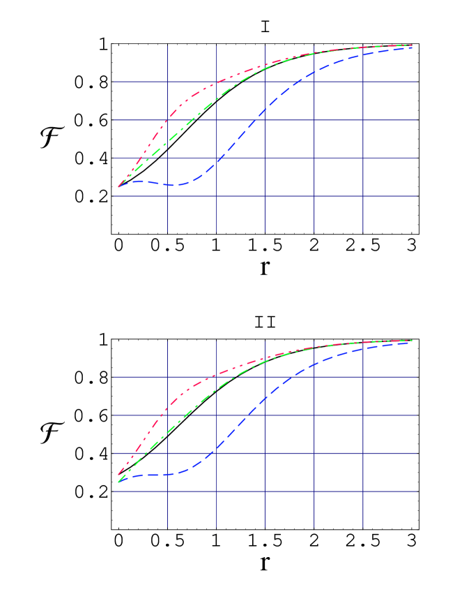
Figure 3.2: Behavior of the fidelity of teleportation $\mathcal{F}$ as a function of the squeezing parameter $r$, with $\phi=\pi$, for two different non-Gaussian input states: The Fock state $|1\rangle$ (Panel I), and the photon-added coherent state $(1+|\beta|^{2})^{-1/2}\hat{a}^{{\dagger}}|\beta\rangle$ (Panel II). We compare the performances obtained by using different two-mode entangled Gaussian and non-Gaussian resources: (a) squeezed state (full line); (b) squeezed Fock state (dashed line); (c) photon-subtracted squeezed state (double-dotted, dashed line); (d) photon-added squeezed state (dot-dashed line). In Panel II the value of the coherent amplitude of the input photon-added coherent state is fixed at $\beta=0.3$.

In Panel I, we observe that both the degaussified resources lead to an improvement of the fidelity with respect to the Gaussian resource. The photon-subtracted squeezed resource again performs better than the photon-added resource; while the squeezed Fock state yields the poorest performance when compared to all the resources. From Panel II we see that once more the photon-subtracted resource yields the best performance for any fixed squeezing parameter; that the photon-added squeezed resource allows for a very modest improvement in the fidelity with respect to the squeezed Gaussian reference for small squeezing.

Differently from the teleportation of Gaussian inputs (see fig. (3.1)), the photon-added resource is no worse than the Gaussian state for small squeezing $r$. That the two-mode squeezed Fock state is a poor resource even at a small squeezing seems unusual. Let us recall that the overlap in eq. (2.55) for classical or nearly classical teleportation ($r\,\rightarrow\,0$) in this case is that of a non-Gaussian, pure input state with a mixture of randomly displaced Fock states; not with a single-photon Fock state.

It is interesting to note that teleportation fidelities (for the same squeezing value $r$) are higher for all the resource states when the input is a photon-added coherent input (compare Panels I and II of fig. (3.2)); higher than when the input is the Fock state that is the zero amplitude limit of the photon-added coherent state. The improvement is small, however, for the input and resource states we have considered. This is not unsurprising, given that the photon-added coherent state, at amplitude $|\beta|^{2}\gg 1$ approximates a coherent state. The protocol for CV teleportation seems more suitable for the teleportation of coherent states than for the teleportation of Fock states, at least as far as our chosen definition of fidelity is concerned.

In fig. (3.3) we compare the fidelity of teleportation $\mathcal{F}$ for the case of a squeezed Fock input state and different Gaussian and non-Gaussian resources. Comparing with Panels I and II of fig. (3.2), we see that the qualitative behavior of teleportation is different from both previous examples, and more reminiscent of that for the Gaussian inputs (see fig. (3.1)). This we explain by noting that the one-mode squeezed Fock state is (at $s=0.8$) of a more Gaussian character than the previous examples of Fock state and photon-added coherent state at small amplitudes.

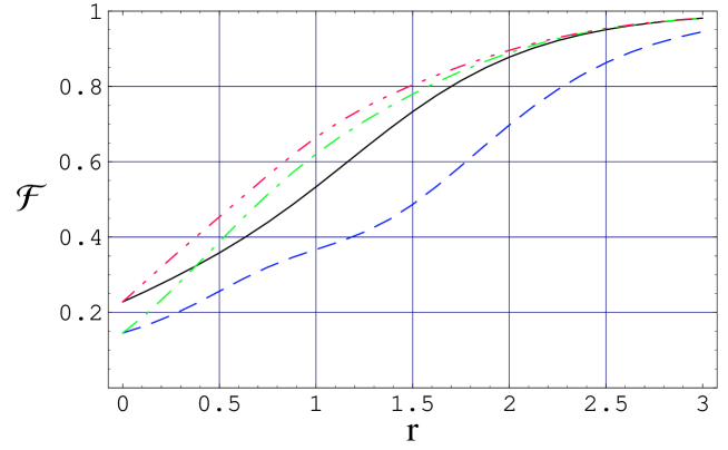
Figure 3.3: Behavior of the fidelity of teleportation $\mathcal{F}$ as a function of the squeezing parameter $r$, with $\phi=\pi$, for the squeezed Fock input state $S(s)\;|\,1\,\rangle$, using different two-mode Gaussian and non-Gaussian entangled resources: (a) squeezed state (full line); (b) squeezed Fock state (dashed line); (c)  photon-subtracted squeezed state (double-dotted, dashed line); (d) photon-added squeezed state (dot-dashed line). The value of squeezing is for the input state is fixed at $s=0.8$.

From all of the above investigations, we conclude that the photon-subtracted squeezed state (eq. (3.7)) is always to be preferred as entangled resource compared either to the Gaussian ones or to non-Gaussian states that are obtained by combining squeezing and photon pumping. The reason explaining this result will become clear in the next sections when we will discuss the general class of states that include as particular cases all the resources introduced so far; and attempt to single out some properties of resource states that are related to improved performance in quantum teleportation.

3.3 Squeezed Bell-like resources for teleportation

In this section we study the fidelity of CV teleportation of the squeezed Bell-like state of eq. (3.13). The class of squeezed Bell-like states includes as special cases all the resources studied so far, as well as the Bell states of the two-dimensional Hilbert space spanned by the vacuum and single-photon Fock states. Part of the analysis will consist in the optimization of the teleportation fidelity with respect to the free superposition parameters of squeezed Bell-like states. The optimal squeezed Bell-like state (for a given input state) can always point the way to an adequate (if not optimal) choice of technically feasible resources for teleportation; and to the further sculpturing of such resources. Even if some states in the class of Bell-like states remain out of the reach of experimental realization. Moreover, the study of the properties of a wide class of resources can be unified and interpolated by the use of squeezed Bell-like states, not only regarding teleportation fidelity, but other uses as well.

The teleportation fidelity (eq. (2.55)) is computable in an analytical manner for all the input states considered, using the squeezed Bell-like resource. It is an explicit function $\mathcal{F}(r,\phi,\delta,\theta)$ of the independent parameters $r$, $\phi$, $\delta$ and $\theta$ that describe the squeezed Bell-like resource.

We do not report here the explicit analytic expressions of the fidelities associated to the squeezed Bell-like resource and to each input state, because they are rather long and cumbersome. Some of them are reported in Appendix A.

An explicit analysis has established that all the fidelities are monotonically increasing functions of the squeezing parameter $r$ at maximally fixed phase $\phi=\pi$. In the following we assume that $\phi=\pi$ and $\theta=0$. It can be checked that non vanishing values of $\theta$ do not lead to an improvement of the fidelity in CV teleportation.

3.3.1 Teleportation with a squeezed Bell state

At finite squeezing $r$ and for $\delta=\frac{\pi}{4}$ and $\theta=0$, state (eq. (3.13)) reduces to a squeezed Bell state. This resource is, as we have remarked in subsection 3.1.3 intrinsically nonclassical; as well as having as a $r=0$ limit the Bell state for the two-dimensional Hilbert space spanned by the vacuum and the single-photon Fock state.

We may assess analytically the performance of such an entangled resource as far as teleportation is concerned. In fig. (3.4) we show the behavior of the fidelity as a function of the squeezing parameter $r$, with $\phi=\pi$, $\delta=\frac{\pi}{4}$ and $\theta=0$ for the five different input states considered in the previous Section. It is straightforward to observe that the squeezed Bell state; used as an entangled resource, leads to a relevant improvement of the performance, when compared to all the other Gaussian and non-Gaussian resources that we have investigated in the previous section.

The squeezed Bell state will always have a better performance for Gaussian inputs than non-Gaussian inputs. The ”best” non-Gaussian input, the small amplitude ($|\beta|^{2}=0.09$) photon-added coherent state, shows a noticeable improvement in fidelity with respect to both Fock and squeezed Fock states. This suggests that the CV teleportation protocol will always have a better performance for Gaussian (or approximatively Gaussian) inputs.

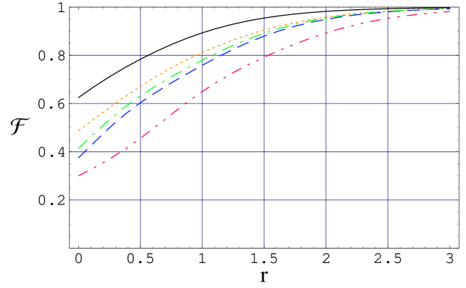
Figure 3.4: Behavior of the fidelity of teleportation $\mathcal{F}(r,\phi,\delta,\theta)$ associated to the squeezed Bell resource with $\phi=\pi$, $\delta=\frac{\pi}{4}$, $\theta=0$, plotted as a function of the squeezing parameter $r$ for the following input states: (a) coherent state (full line); (b) squeezed state $|s\rangle=S(s)|0\rangle$, with $s=0.8$ (dotted line); (c) Fock state $|1\rangle$ (dashed line); (d) photon-added coherent state $(1+|\beta|^{2})^{-1/2}\hat{a}^{{\dagger}}|\beta\rangle$, with $\beta=0.3$ (dot-dashed line); (e) squeezed Fock state $|s\rangle=S(s)|1\rangle$, with $s=0.8$ (double-dotted, dashed line).

3.3.2 Optimized squeezed Bell-like resources for teleportation

We proceed to maximize, for every input state, the fidelity $\mathcal{F}(r,\pi,\delta,0)$ over the Bell-superposition angle $\delta$. At a fixed squeezing $r=\tilde{r}$, we define the optimized fidelity as

$$\mathcal{F}_{opt}(\tilde{r})\,=\,\max_{\delta}\;\mathcal{F}(\,\tilde{r},\,\pi,\,\delta,\,0\,)\;.$$ (3.20)

For a coherent state input the maximization of $\mathcal{F}(\,r,\pi,\delta,0\,)$, at fixed $r$, leads to the following determination for the optimal Bell-superposition angle $\delta_{max}^{(c)}$;

$$\delta_{\,max}^{(c)}\,=\,\frac{1}{2}\,\arctan(1\,+\,e^{-2\,r}\,)$$ (3.21)

For a single-photon Fock state input, the optimal angle is given by

$$\delta_{\,max}^{(F)}\,=\,\frac{1}{2}\,\arctan\left(\frac{e^{-2\,r}(1-e^{2\,r}+e^{4\,r}+3e^{6\,r})}{3(e^{2\,r}-1)^{2}}\right)$$ (3.22)

We report, in fig. (3.5) the behavior of the optimized fidelities $\mathcal{F}_{opt}(r)$ as functions of $r$ for all the input states considered in this chapter. In all: coherent state, squeezed vacuum, single-photon Fock state, photon-added coherent state and squeezed single-photon Fock state.

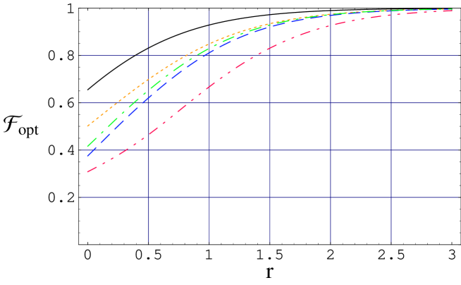
Figure 3.5: Plot of the fidelity $\mathcal{F}_{opt}(r)$, using optimal squeezed Bell-like resources, as a function of $r$ for the following input states: (a) coherent state (full line); (b) squeezed vacuum $|\,s\,\rangle$, with $s=0.8$ (dotted line); (c) single-photon Fock state $|\,1\,\rangle$ (dashed line); (d) photon-added coherent state $(1+|\beta|^{2})^{-1/2}\hat{a}^{{\dagger}}|\beta\rangle$, with $\beta=0.3$ (dot-dashed line); (e) squeezed Fock state $|1,\,s\,\rangle$, with $s=0.8$ (double-dotted, dashed line).

A relevant improvement of the fidelity is observed in all cases, even at vanishing squeezing, due to the persistent nonclassical character of the optimal, squeezed Bell-like entangled resource; even in the limit $r\rightarrow 0$.

The Gaussian states, and the photon-added coherent state show higher teleportation fidelities than the wholly non-Gaussian states for all $r$ values. This result; together with similar results in subsections 3.2.2 and 3.3.1 strongly suggest that some local operations; a suitable displacement, for instance on a non-Gaussian input state previous to CV teleportation might improve the fidelity of teleportation, for any resource used.

To quantify the increase in the probability of success for teleportation when we use the optimal squeezed Bell-like state for a resource; we define a relative fidelity coefficient $\Delta\,\mathcal{F}(r)$; relative with respect to the fidelity $\mathcal{F}_{ref}(r,\pi)$ achieved using with one of the ”special case” resources as a benchmark . A natural definition of such a relative quantity is

$$\Delta\,\mathcal{F}(r)\,=\,\frac{\mathcal{F}_{\,opt\,}(r)-\mathcal{F}_{\,ref\,}(r,\pi)}{\mathcal{F}_{\,ref\,}(r,\pi)}$$ (3.23)

In fig. (3.6), we plot the relative fidelity $\Delta\,\mathcal{F}(r)$ as a function of the squeezing parameter $r$ for two different choices of benchmark resources that we have deemed the most interesting, given the high values of the fidelities obtained when using them. In Panel I, the benchmark resource is the Gaussian two-mode squeezed vacuum; in Panel II the benchmark resource is the non-Gaussian two-mode photon-subtracted squeezed state.

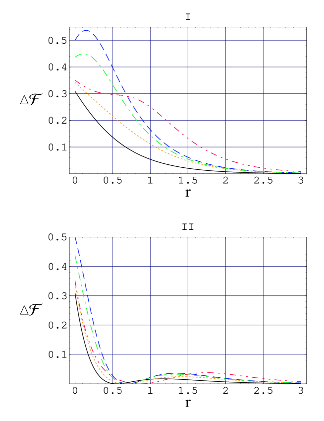
Figure 3.6: Behavior of the relative fidelity $\Delta\mathcal{F}(r)$ using an optimal squeezed Bell-like resource, as a function of $r$ for the following input states: (a) coherent state (full line); (b) squeezed state $|s\rangle$, with $s=0.8$ (dotted line); (c) single-photon Fock state $|1\rangle$ (dashed line); (d) photon-added coherent state $(1+|\beta|^{2})^{-1/2}\hat{a}^{{\dagger}}|\beta\rangle$, with $\beta=0.3$ (dot-dashed line); (e) squeezed Fock state $|1,s\rangle$, with $s=0.8$ (double-dotted, dashed line). In Panel I the benchmark resource is the two-mode squeezed vacuum; in Panel II the benchmark resource is the two-mode photon-subtracted squeezed state.

In Panel I of fig. (3.6) we see that at fixed squeezing, the use of optimized squeezed Bell-like resources leads to a strong percent enhancement of the teleportation fidelity (up to more than $50\%$) with respect to that attainable exploiting the standard two-mode squeezed vacuum. The greatest relative improvements, and the maxima in relative fidelity, occur in the teleportation of the non-Gaussian inputs, particularly with the Fock state and the photon-added coherent state (for which the relative improvement is not as great). Obviously, in the asymptotic limit of very large squeezing, the two resources converge to unity teleportation efficiency, as the resources themselves converge to EPR states.

Panel II shows that the use of the optimized squeezed Bell-like resource leads to a significant advantage with respect to the use of the photon-subtracted squeezed state resource for low values (up to $r\simeq 0.5$) of the squeezing. The different curves corresponding to the different input states, exhibit the same qualitative behavior; however, the greater relative improvements are those for the fidelity of teleportation of non-Gaussian inputs, particularly the Fock state and the photon-added coherent state (again, with a lesser relative improvement than the Fock state). Starting from large values, $\Delta\mathcal{F}(r)$ decreases monotonically and vanishes at different points in the interval $[0.5\leq r\leq 0.9]$. After vanishing, the relative fidelity exhibits peaks at different intermediate values of the squeezing, before vanishing asymptotically for large values of $r$. Unsurprisingly; for these minima values of $r=\bar{r}$ such that $\Delta\mathcal{F}(\bar{r})=0$, the optimized Bell-like state and the photon-subtracted squeezed state are identical.

3.4 A comparison of entanglement, non-Gaussian character and Gaussian affinity of resource states

In this section, we analyze the characteristics of the resource states studied in this chapter, to determine which properties of the resources have an influence on teleportation fidelity. Particularly, we study the entanglement and non-Gaussian character of optimized Bell-like states and compare them with those of photon-subtracted and photon-added two mode squeezed states. This comparison is to be particularly illuminating, given the difference in teleportation fidelity obtained using these degaussified states as resources; and given the very different characteristics (obvious for $r\rightarrow 0$) of these two types of resources that seem otherwise similar.

First, we study entanglement, as given for pure states by the von Neumann Entropy. Then, we study non-Gaussian character as given by a measure of the distance between the resource under study and a reference Gaussian state having the same covariance matrix and first order averages as the resource. Thirdly, we define and study Gaussian affinity as given by the overlap of the resource and a two-mode squeezed vacuum, maximized over the squeezing parameter of the latter.

We analyze these measures in conjunction for the resources above mentioned, paying special attention to the behavior of these measures for optimized Bell-like states.

3.4.1 The von Neumann entropy of non-Gaussian resources

The bipartite entanglement; the Schmidt rank of the pure non-Gaussian states chosen for study in this chapter can be quantified in an unique manner using the partial Von Neumann entropy (entropy of entanglement) $E_{vN}$. Given the density operator for the two-mode state $\hat{\rho}$, the von Neumann entropy is equal to the Shannon [78] entropy of the partial traces:

$$E_{vN}=\,-\mathrm{Tr}\left(\,\hat{\rho}^{\,Tr(A)}\>\log_{2}(\hat{\rho}^{\,Tr(A)})\right)\;=\;-\,\mathrm{Tr}\left(\,\hat{\rho}^{\,Tr(B)}\>\log_{2}(\hat{\rho}^{\,Tr(B)})\right)$$ (3.24)

where the partial traces are indicated by $\hat{\rho}^{\,Tr(A)}=\,\mathrm{Tr}_{A}(\hat{\rho})$, and by $\hat{\rho}^{\,Tr(B)}=\,\mathrm{Tr}_{B}(\hat{\rho})$

To simplify calculations involving powers of the density operator of the aforementioned resource states (see section 3.1), the series expansion for the logarithmic function in eq. (3.24) has been truncated to the first-order.

For the two-mode squeezed Fock and the degaussified states, the von Neumann entropy depends only on the modulus $r$ of the squeezing parameter $\zeta$. It is plotted in fig. (3.7) and compared to that of the Gaussian two-mode squeezed state.

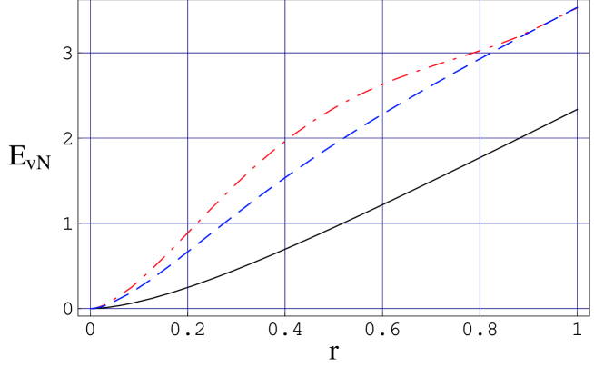
Figure 3.7: Behavior of the von Neumann entropy $E_{vN}$ for two-mode squeezed Fock, two-mode photon-added and two-mode photon subtracted squeezed states, as a function of the modulus squeezed parameter $r$. The upper curve (dot-dashed line) corresponds to the squeezed Fock state $|r\,;1\,,1\,\rangle$; the intermediate curve (dashed line) corresponds equivalently to the photon-subtracted squeezed state $|1^{(-)}\,,1^{(-)}\,;\>r\,\rangle$ and to the photon-added $|1^{(+)}\,,\,1^{(+)}\,;\>r\rangle$ squeezed state . The lower curve corresponds to the Gaussian two-mode squeezed state $|\,r\,\rangle$.

At a given squeezing, all the non-Gaussian states show an entanglement larger than that of the Gaussian two-mode squeezed vacuum. In the range of experimentally realistic values $0<r<1$ of the squeezing, the two-mode squeezed Fock state is the most entangled state. Moreover, the photon-added and the photon-subtracted two-mode squeezed states exhibit exactly the same amount of entanglement at any $r$.

However, the results in subsections 3.2.1 and 3.2.2 indicate that, for a given squeezing $r$, a higher von Neumann Entropy (and greater entanglement) does not correspond to a higher teleportation fidelity. The two-mode squeezed Fock state obtains the smallest teleportation fidelities of any resource while having the greatest von Neumann entropies. And the photon-added two-mode squeezed state obtains lower teleportation fidelities than the photon-subtracted state, even if they are indistinguishable by their von Neumann entropy.

The von Neumann entropy of the general squeezed Bell-like states is plotted in fig. (3.8). In panel I we plot $E_{vN}$ as a function of $r$ and $\delta$. In panel II, we can observe how the regular, oscillating behavior of the entropy for the Bell-like state $(r=0)$ becomes gradually deformed by the optical pumping $(r\neq 0)$, leading to a peculiar pattern of correlation properties for the squeezed Bell-like state.

Note that for $\delta=0$ and $\delta=\pi/2$, we have the von Neumann entropy of the Gaussian state and the squeezed Fock state, respectively in Panel II of fig. (3.8).

The squeezed Bell-like states have maxima of von Neumann Entropy for $r\rightarrow 0$ near $\pi/4$ and $3\pi/4$. However, it suffices to evaluate eqs. (3.21) and (3.22) for $r=0$ (recall that the Bell-like state is entangled even if it is not squeezed) to realize that, while the optimal fidelity for the teleportation of Fock state inputs is obtained for $\delta^{(F)}_{max}(r=0)=\pi/4$ (the Bell state of discrete variables settings), this is not the case for the coherent state inputs, with $\delta^{(C)}_{max}(r=0)=0.554$. Even in the case of Bell state resources for CV teleportation, the greatest von Neumann entropy does not maximum determine fidelities for certain classes of states.

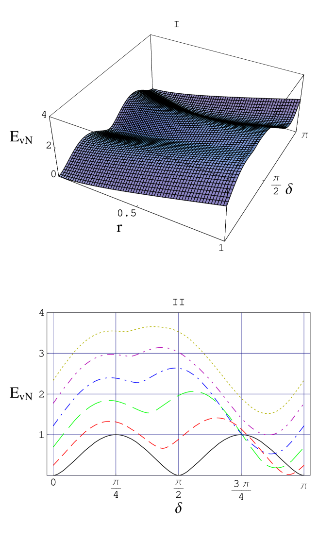
Figure 3.8: The von Neumann entropy $E_{vN}$ for the squeezed Bell-like state as a function of its defining parameters $r$ and $\delta$. Panel I displays the three-dimensional plot of $E_{vN}$. Panel II displays two-dimensional projections at fixed squeezing strength $r$. Curves from bottom to top correspond to the different sections of $E_{vN}$ as functions of $\delta$ for $r=0,\,0.2,\,0.4,\,0.6,\,0.8,\,1$.

3.4.2 Optimized squeezed Bell-like resources: A comparison of von Neumann entropies

In fig. (3.9), we show the behavior of the von Neumann entropy $E_{vN}$ for two different squeezed Bell-like resources; the first one optimized for the teleportation of an input coherent state, with $\delta_{max}^{(c)}(r)$ (see eq. (3.21)); the second one optimized for the teleportation of a single-photon Fock state, with $\delta_{max}^{(F)}(r)$ (see eq. (3.22)). This behavior is compared with that of the von Neumann entropy of both the degaussified states. The intersections between the curves in the figure correspond to the values os squeezing $\bar{r}$ for which the squeezed Bell-like state reduces to a photon-subtracted or to a photon-added squeezed state.

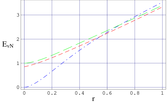
Figure 3.9: The von Neumann entropy $E_{vN}$ for the optimized squeezed Bell-like state, as a function of $r$. Dashed line: Optimized resource for a coherent state input, $\delta=\delta_{max}^{(c)}$; Long dashed line: Optimized resource for a Fock state input, $\delta=\delta_{max}^{(F)}$. The von Neumann entropy of the degaussified states is reported for comparison purposes (dot-dashed line).

It can be noticed in the range $0<r<\bar{r}$; in which the fidelity of teleportation using optimized Bell-like resources is substantially higher than that for the photon-subtracted squeezed resource (see fig. (3.6), Panel II), that the entanglement (quantified by the von Neumann Entropy) of the squeezed Bell-like state is always larger than that of the photon-subtracted (and photon-added) squeezed states. Therefore, a partial explanation of the better performance of squeezed Bell-like resources lies in their higher degree of entanglement compared to other non-Gaussian resources at lower levels of squeezing. However, from the graphs it can be seen that for $r>\bar{r}$ the entanglement of photon-subtracted and/or added resources is larger; nevertheless, the fidelity of teleportation is below that associated to optimized squeezed Bell-like resources. Much lower, in the case of the photon-added resource, we remark.

Therefore, entanglement is not the only parameter necessary to determine the teleportation performance of different non-Gaussian resources. The example chosen here validates this conclusion specially well; nonetheless because the squeezed Bell-like state is a generalization of degaussified resources, that reduces to a degaussified resource for certain values of the superposition angle $\delta$.

3.4.3 The non-Gaussianity: A character measure

We have concluded that entanglement alone does not suffice to determine the teleportation fidelity for a non-Gaussian resource. We have seen that the two-mode squeezed Fock state, the wholly non-Gaussian resource having the highest entanglement of the resources studied in this work, performs poorly as a teleportation resource. We have seen that the degaussified states, resources of a different character; but equal entanglement, perform the teleportation of the same input with very different fidelities. We have seen that the optimal choices of squeezed Bell-like resources for teleportation (at a fixed squeezing $r$) do not always correspond to maximal entanglement. We have seen notable differences in the teleportation fidelities of Gaussian and non-Gaussian inputs, using the same resource.

It is natural, as we study non-Gaussian resources and observe improvements in teleportation fidelity over Gaussian resources, to look for a quantification of the non-Gaussian character of the different resources we have considered, and in general of the optimized squeezed Bell-like resources in order to compare their performance in teleportation with respect to both this quantity and the entanglement in conjunction. The task is to define a reasonable measure of non-Gaussianity that is endowed with some nontrivial operative meaning.

Recently, inspired by work [6] on the extremal nature of Gaussian states at fixed covariance matrix; a measure of non-Gaussianity has been introduced in terms of the Hilbert-Schmidt distance between a given non-Gaussian state and a reference Gaussian state with the same covariance matrix [79]. Given a generic state with density operator $\hat{\rho}$; its non-Gaussian character can be quantified through the distance $d_{nG}$ between $\hat{\rho}$ and the reference Gaussian state $\hat{\rho}_{G}$, defined according to the following relation:

$$d_{nG}=\frac{\mathrm{Tr}((\,\hat{\rho}\,-\,\hat{\rho}_{G}\,)^{2})}{2\>\mathrm{Tr}(\,\hat{\rho}^{2}\,)}=\frac{\mathrm{Tr}(\,\hat{\rho}^{2}\,)\>+\>Tr(\,\hat{\rho}_{G}^{2}\,)\>-\>2\,\mathrm{Tr}(\,\hat{\rho}\,\hat{\rho}_{G})\,}{2\>\mathrm{Tr}(\,\hat{\rho}^{2}\,)},$$ (3.25)

where the Gaussian state $\rho_{G}$ is completely determined by the same covariance matrix and the same first order average values of the quadrature operators associated to state $\rho$.

Using this definition, in fig. (3.10) we report the behavior of the non-Gaussianity $d_{nG}$ for the squeezed Bell-like state.

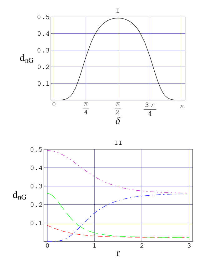
Figure 3.10: Non-Gaussianity measure $d_{nG}$ for the squeezed Bell-like state. Panel I shows $d_{nG}$ for the squeezed Bell-like state as a function of $\delta$, for arbitrary $r$. Panel II shows $d_{nG}$ for the squeezed Bell-like state as a function of $r$, for $\delta$ fixed at the optimized values for coherent state inputs $\delta=\delta_{max}^{(C)}$ (dashed line); and $\delta=\delta_{max}^{(F)}$ for Fock state inputs (long dashed line). For comparison, the values of $d_{nG}$ for the photon-subtracted resource (dot-dashed line) and photon-added resource (double dotted, dashed line) are also reported.

The quantity $d_{nG}$ depends only on the superposition angle $\delta$ of the squeezed Bell-like state (see Panel I), as the non-Gaussianity of the state cannot change under squeezing operations; the squeezing induced on the state measured would translate into squeezing of the reference Gaussian state. For $\delta$ in the interval $[0,\pi]$, $d_{nG}$ attains its maximum at $\delta=\frac{\pi}{2}$: At that point, the squeezed Bell-like state reduces to a two-mode squeezed Fock state. It is expected for a (two-mode squeezed) Fock state to be more non-Gaussian than a (two-mode squeezed) superposition of the vacuum and of a Fock state.

In Panel II, we plot the behavior of $d_{nG}$ for the squeezed Bell-like resources optimized for the teleportation of a coherent state input and a single-photon Fock state input, respectively, with $\delta=\delta_{max}^{(C)}$ and $\delta=\delta_{max}^{(F)}$. For comparison, we plot as well the non-Gaussianity $d_{nG}$ for the photon-added and the photon-subtracted squeezed states. The intersection points occur once again at the points $\bar{r}$ where the optimized squeezed Bell-like states reduce to the photon-subtracted squeezed states. For $r$ in the range $[0,\bar{r}]$, the optimized squeezed Bell-like resources are not only more entangled; they are more non-Gaussian than the photon-subtracted squeezed states. We note that for $\lim_{r\rightarrow\infty}\delta_{max}^{(C)}\,=\,\lim_{r\rightarrow\infty}\delta_{max}^{(F)}\,=\,1$. Thus, for very large squeezing the two optimized squeezed Bell-like resources tend to the state $\widehat{S}_{AB}(-r)\;\{\cos\frac{\pi}{8}|\,0\,,\,0\,\rangle_{AB}\,+\,\sin\frac{\pi}{8}\,|\,1\,,\,1\,\rangle_{AB}\}$, exhibiting a dominating Gaussian component. On the other hand, for large $r$, the squeezed photon-added and photon-subtracted squeezed states asymptotically tend to a squeezed Bell state (corresponding to $\delta_{max}=\frac{\pi}{4}$), which has balanced Gaussian and non-Gaussian contributions. While for smaller values of $r$, they have very different values of non-Gaussianity; which is not surprising if we recall the enormous difference in character of these states for $r\rightarrow\,0$.

It is also remarkable that, for $r$ in the range $[0,\bar{r}]$, that the optimal squeezed Bell-like resources for teleportation of the non-Gaussian Fock state ($\delta_{max}^{(F)}$) have a much higher non-Gaussianity than those optimal squeezed Bell-like resources for teleportation of the Gaussian coherent state ($\delta_{max}^{(C)}$). This might be understandable for completely ”classical” teleportation with an squeezed resource of the type studied so far, where fidelity is just the overlap of the input state $in$ with a mixture of states constituted of different instances of random displacements of mode $B$. But this is not the case here; the squeezed Bell-like resources are always entangled even for $r=0$, with the exception of some trivial choices for $\delta$.

3.4.4 The Gaussian resource affinity

We have developed a non-Gaussianity measure for entangled resources that is in effect a distance between the resource state we are studying and a Gaussian state of the same covariance matrix. But this Gaussian reference is different for every resource studied, and the interest of such a measure lies in making comparisons of the non-Gaussianity for different non-Gaussian resources. Moreover, we do not know that the Gaussian state constructed for every particular measure is a resource for teleportation, for it is not described as such.

Observing that the squeezed Bell-like states and the photon-added and photon-subtracted squeezed states are all obtained through a degaussification protocol from a pure squeezed state, one could modify the definition of eq. (3.25) by taking the two-mode squeezed vacuum $|\,\zeta^{\prime}\,\rangle_{AB}$ $(\zeta^{\prime}=r^{\prime}\,e^{i\phi^{\prime}})$ as the universal reference Gaussian state $\hat{rho}_{G}$. This choice makes it possible to compare our non-Gaussian resources to an unique reference that is also a well studied teleportation resource. This will be particularly important if we are to analyze measures of non-Gaussianity, teleportation fidelities and von Neumann entropies together.

Adopting this modified definition, and observing that the non-Gaussian states to be compared and the reference Gaussian state are all pure, eq. (3.25) reduces to $d_{nG}\,=\,\min_{r^{\prime},\,\phi^{\prime}}\{1-Tr[\hat{\rho}\,\hat{\rho}_{G}]\}$, where the minimization is constrained to run over the squeezing parameters $\zeta^{\prime}$ of the reference twin-beam. However, it turns out that this modified definition provides results and information qualitatively analogous to those obtained by applying the original definition.

There is still one, and apparently opposite property that plays a crucial role in the sculpturing of an optimized non-Gaussian entangled resource. From figs. (3.9) and (3.10) we see that at sufficiently large squeezing the photon-added and photon-subtracted squeezed resources have entanglement comparable to that of the optimized squeezed Bell-like states and, moreover, possess stronger non-Gaussianity. Yet they are not able to perform better than the optimized Bell-like resources. This fact can be understood as follows, leading to a definition of squeezed vacuum affinity: It is well known that the Gaussian two-mode squeezed state in the limit of infinite squeezing realizes the EPR state which is the equivalent of the Bell (eq. (1.64)) state for two-dimensional systems. These two ideal resources, respectively in the CV and discrete variables case, allow perfect quantum teleportation with maximal fidelity. Therefore, we argue that, even when exhibiting enhanced properties of non-Gaussianity and entanglement, any efficient resource for CV quantum information tasks should enjoy a further property, i.e. to resemble the form of a two-mode squeezed vacuum as much as is possible, in the large $r$ limit. The squeezed vacuum affinity can be quantified by the following maximized overlap:

$$\mathcal{G}\,=\,\max_{s}|\,_{AB}\langle\,-s\,|\,\psi_{res}(r)\,\rangle_{AB}\,|^{2}$$ (3.26)

where $|\,-s\,\rangle_{AB}$ is a two-mode squeezed vacuum with real squeezing parameter $-s$, and $|\,\psi_{res}(r)\,\rangle_{AB}$ is any entangled two-mode resource that depends on the squeezing parameter $r$. This definition applies straightforwardly to the photon-added and photon-subtracted squeezed resources, and as well to the squeezed Bell-like resources whenever they are optimized with respect to a particular input state. The maximization over $s$ is imposed in order to determine, at fixed $r$, the two-mode squeezed vacuum that is most affine to the non-Gaussian resource being considered.

In fig. (3.11) we study the behavior of the overlap $\mathcal{G}$ as a function of the squeezing $r$ for different non-Gaussian entangled resources.

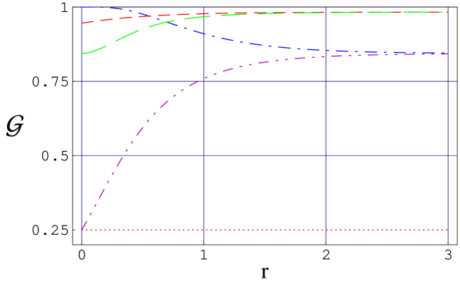
Figure 3.11: Maximized overlap $\mathcal{G}$ between a two-mode squeezed vacuum and different non-Gaussian entangled resources as a function of $r$: squeezed Bell-like state with $delta$ fixed at the optimized value $\delta=\delta_{max}^{(c)}$ for coherent state inputs (dashed line); the same state with $delta$ fixed at the optimized value $\delta=\delta_{max}^{(F)}$ for Fock state inputs (long dashed line). For comparison purposes the maximized overlap with the photon-subtracted squeezed state (dot-dashed line); photon-added squeezed state (double-dotted, dashed line); and the single-photon squeezed Fock state (dotted line) are displayed as well.

Comparing fig. (3.10) and fig. (3.11) we can see that the behaviors of the non-Gaussianity and squeezed vacuum affinity seem to be complementary. Take the curve for any one state and observe growth and asymptotic behaviors. For example the photon added resource: non-Gaussianity approaches its asymptotic value from above; it is obviously a convex function; two-mode vacuum affinity approaches its asymptotic value from below, and it is a concave function.

Observe (in fig. (3.11)) that the photon-subtracted and photon-added resources that have equal entanglement for every $r$ are perfectly distinguishable by squeezed vacuum affinity.

In fig. (3.11), the greatest affinity $\mathcal{G}$ is always achieved at large values of the squeezing parameter by the optimized squeezed Bell-like resources, while the lowest, constant affinity is always exhibited by the squeezed Fock states. Observe additionally that the Squeezed Bell-like resource optimized for coherent states ($\delta_{max}^{(c)}$) has a higher affinity than the resource optimized for Fock states (($\delta_{max}^{(F)}$)), specially for the smaller values of $r$.

In conclusion, optimized squeezed Bell-like resources are the ones that in all squeezing regimes are closest to the simultaneous maximization of entanglement, non-Gaussianity, and affinity to the two-mode squeezed vacuum. The optimized interplay of these three properties explains the ability of squeezed Bell-like states to yield better performances, when used as resources for CV quantum teleportation, in comparison both to Gaussian resources at finite squeezing and to the standard degaussified resources such as the photon-added and the photon-subtracted squeezed states.

3.5 Experimental generation of degaussified and squeezed Bell-like states

While two-mode Gaussian squeezed states are currently produced in the laboratory, the experimental generation of non-Gaussian states in quantum optics is still a complex task, as it requires the availability of large nonlinearities and/or the arrangement of proper apparatus for conditional measurements. Nevertheless, some truly remarkable realizations of single-mode non-Gaussian states have been recently carried out through the use of parametric amplification plus postselection [13, 14, 15]. Recently, by a generalization of the experimental setup used in Ref. [15] to a two-mode configuration, a method has been proposed [3] for the generation of a certain class of two-mode photon-subtracted states.

Here, in an analogous manner to that of ref. [13], we propose a possible experimental setup for the generation of the degaussified states (eqs. (3.8) and (3.7)), and of the squeezed Bell-like states (eq. (3.13)). The scheme, based on a configuration of cascaded crystals, is depicted in fig. (3.12).

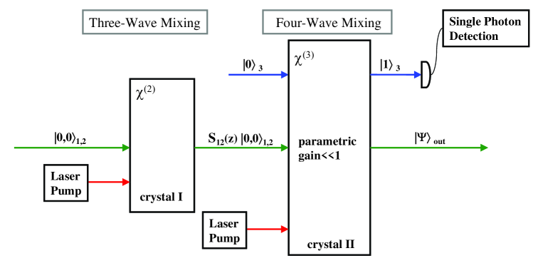
Figure 3.12: Scheme for the generation of the photon-subtracted squeezed state and of the photon-added squeezed state. Two nonlinear crystals are used in a cascaded configuration. The first $\chi^{(2)}$-crystal is part of a three-wave mixer, acting as a parametric amplifier for the production of a two-mode squeezed state. The squeezed state seeds the successive nonlinear process, a four-wave mixing interaction occurring in a $\chi^{(3)}$-crystal. A final conditional measurement reduces the multiphoton state to a photon-subtracted (or added) squeezed state $|\,\Psi\,\rangle_{out}$.

In the first stage, by means of a three-wave mixer, functioning as a parametric amplifier, a two-mode squeezed state $|\zeta\rangle_{12}=\widehat{S}_{12}(\zeta)|0,0\rangle_{12}$ is produced. In the second stage, a four-wave mixing process takes place in a crystal with third order nonlinear susceptibility $\chi^{(3)}$. We consider two possible multiphoton interactions, in the travelling wave configuration, described by the following Hamiltonian operators;

$$\widehat{H}_{I}^{(A)}\,= \,\kappa_{A}\hat{a}_{1}\hat{a}_{2}\hat{a}_{3}^{{\dagger}}\,+\,\kappa_{A}^{*}\hat{a}_{1}^{{\dagger}}\hat{a}_{2}^{{\dagger}}\hat{a}_{3}\;,$$ (3.27)

$$\widehat{H}_{I}^{(B)}\,= \,\kappa_{B}\hat{a}_{1}^{{\dagger}}\hat{a}_{2}^{{\dagger}}\hat{a}_{3}^{{\dagger}}\,+\,\kappa_{B}^{*}\hat{a}_{1}\hat{a}_{2}\hat{a}_{3}\;,$$ (3.28)

where $\hat{a}_{i}$ $(i=1,2,3)$ denotes three quantized modes of the radiation field. The complex parameters $\kappa_{A}$ and $\kappa_{B}$ are proportional to the third order nonlinearity and to the amplitude of an intense coherent pump field, treated classically in the regime of parametric approximation. The two-mode squeezed state seeds modes $1$ and $2$; mode $3$ is initially in the vacuum state $|\,0\,\rangle_{3}$; mode $4$ is the classical pump. Energy conservation and phase matching are assumed throughout. Let us remark that, due to the typical orders of magnitudes of the third order susceptibilities, the parametric gains are very small $|\,\kappa_{A}\,|\,,\;\;|\,\kappa_{B}\,|\ll 1$. The propagation (time evolution) in the crystal yields $|\,\Psi_{I}^{(L)}\,\rangle\,=\,\exp\{-\,i\,t\,\widehat{H}_{I}^{(L)}\}|\,\zeta\,\rangle_{12}\;|0\rangle_{3}$ $(L=A,B)$. Truncating the series expansion of the evolution operator at the first order in $\tilde{\kappa}_{L}=\,-\,i\,t\,\kappa_{L}$ we get

$$|\,\Psi_{I}^{(A)}\,\rangle\,\approx \,\{1\,+\,\tilde{\kappa}_{A}\,\hat{a}_{1}\hat{a}_{2}\hat{a}_{3}^{{\dagger}}\}\,|\,\zeta\,\rangle_{12}\,|\,0\,\rangle_{3}$$ (3.29)

$$|\,\Psi_{I}^{(B)}\,\rangle\,\approx \,\{1\,+\,\tilde{\kappa}_{B}\,\hat{a}_{1}^{{\dagger}}\hat{a}_{2}^{{\dagger}}\hat{a}_{3}^{{\dagger}}\}\,|\,\zeta\,\rangle_{12}\,|\,0\,\rangle_{3}$$ (3.30)

Finally, a conditional measurement is performed on mode $3$, consisting in a single-photon detection; a projection onto the state $|1\rangle_{3}$. The postselection reduces the states of eq. (3.29) and eq. (3.30) to the states of eq. (3.7) and eq. (3.8), respectively. It is worth noting that the low values of the parametric gains do not affect the implementation of the process. In fact, it is analogous to require low reflectivity of a beam splitter to generate photon-subtraction (addition) by using linear optics.

Regarding the production of the squeezed Fock state (eq. (3.1)), it can be generated, in principle, by seeding a parametric amplifier with a single-photon states in the two modes.

Let us now turn to the experimental generation of the squeezed Bell-like states (eq. (3.13)). They can be engineered by using the same setup illustrated in fig. (3.12), and by simultaneously realizing inside the nonlinear crystal the processes corresponding to the interactions in eq. (3.27) and eq. (3.28). In this case the fundamental requirements are that of energy conservation and phase-matching for each multiphoton interaction must hold simultaneously at each stage. This condition can be satisfied by suitably exploiting the phenomenon of birefringence in a negative uniaxial crystal [82]. In particular, the following set of equations must hold:

$$\Omega_{1}=\omega_{1}+\omega_{2}+\omega_{3}$$

$$K_{1}^{ext}=k_{1}^{ord}+k_{2}^{ord}+k_{3}^{ext}$$ (3.31)

$$\Omega_{2}+\omega_{1}+\omega_{2}=\omega_{3}$$

$$K_{2}^{ord}+k_{1}^{ord}+k_{2}^{ord}=k_{3}^{ext}$$ (3.32)

where $\omega_{j}$ and $k_{j}^{\lambda}$ $(j=1,2,3)$ represent the frequencies and the wave vectors of the quantized modes with polarization $\lambda$; $\Omega_{j}$ and $K_{j}^{\lambda}$ $(j=1,2)$ represent the frequencies and the wave vectors of the classical pump fields; the superscript $ord$ and $ext$ denote, respectively, the ordinary and extraordinary polarizations for the propagating waves. A collinear configuration is assumed for the geometry of propagation inside the crystal. Then, at fixed $\omega_{1}$ and $\omega_{2}$, the energy conservation relations, the type-II phase matching condition in eq. (3.31), and the type-I phase matching condition in eq. (3.32) can be, in principle, satisfied by a suitable choice of $\omega_{3}$, $\Omega_{1}$, $\Omega_{2}$, and of the phase-matching angle between the direction of propagation and the optical axis. Various examples of such simultaneous multiphoton processes have been demonstrated both theoretically and experimentally [1, 83, 84, 85]. The final conditional measurement on mode $3$ yields the superposition state

$$|\Psi_{I}\rangle\,\approx\,\tilde{\kappa}_{A}\,\hat{a}_{1}\,\hat{a}_{2}\,\widehat{S}_{12}(\zeta)\>|\,0\,,\,0\,\rangle_{12}\;+\;\tilde{\kappa}_{B}\,\hat{a}_{1}^{{\dagger}}\,\hat{a}_{2}^{{\dagger}}\,\widehat{S}_{12}(\zeta)\>|\,0\,,\,0\,\rangle_{12}$$ (3.33)

By applying a standard Bogoliubov transformation and after a little algebra, it is straightforward to show that the superposition state (eq. (3.33)) reduces to the squeezed Bell-like state (eq. (3.13)) if

$$c_{1}= \,-(e^{-i\phi}\,\tilde{\kappa}_{B}\,\tanh(r)\>+\>e^{i\,\phi}\,\tilde{\kappa}_{A})$$

$$c_{2}= \,\tilde{\kappa}_{B}\>+\>e^{2\,i\,\phi}\,\tilde{\kappa}_{A}\,\tanh(r)$$ (3.34)

The latter conditions can be successfully implemented by observing that the complex parameters $\tilde{\kappa}_{A}$ and $\tilde{\kappa}_{B}$ can be controlled to a very high degree by means of the amplitudes of the external classical pumps.

Chapter 4 Teleportation with ”truncated” Gaussians and squeezed cat-like resources

We introduce, in section 4.1, the class of squeezed symmetric superpositions of Fock states [37] as a further generalization of the squeezed Bell-like states (see eq. (3.13)), and apply to them the optimization procedure defined in ref. [24] and used in chapter 3; obtaining a maximal fidelity of teleportation of a given input, over the superposition parameters defining the character of the resource. We find that the optimal resources for teleportation in this class of states are necessarily constrained to be second-order ”truncations” of the two-mode squeezed Gaussian states (see eq. (3.12)).

In section 4.2 we introduce the class of squeezed cat-like states; optimize this class of states for maximal fidelity of teleportation over the available parameters, and compare results with those obtained in the previous section.

4.1 Truncated squeezed Gaussians: Symmetric Superpositions of Fock States and Bell-like states

In chapter 3, the squeezed Bell-like states have been exploited as non-Gaussian entangled resources that generalize the search for an optimal teleportation fidelity among various classes of input states, which these states interpolate. The squeezed Bell-like states (eq. (3.13)) can be formulated as the application of the two-mode squeezing operator (eq. (1.41)) to a general superposition of the two-mode vacuum and two-mode single-photon Fock state (having two photons one in each mode), similar to a Bell state of discrete variables (eq. (1.64)).

The optimization of teleportation fidelity over the superposition parameters yields a remarkable enhancement in the success probability of teleportation for various input states [24] using squeezed Bell-like states. In this section, we produce a further generalization on the squeezed Bell-like states deemed the Squeezed Symmetric Superposition of Fock states [37]; and show that the optimal fidelity choice for this new class of states (and all the squeezed Bell-like states) can be regarded as truncations (on the photon number) of two-mode squeezed vacuums.

4.1.1 Definition: truncated Gaussians

The squeezed Bell-like states, having only two superposition components and the constraint of normalization, can be parameterized in alternative ways. A parameterization based on the first order ($n=1$) truncation (see eqs. (1.43) and (3.12)) of the two-mode squeezed vacuum state is possible. Take a trivial generalization of the aforementioned expressions,

$$|-(r+s)\,\rangle_{AB}\,=\, \widehat{S}_{AB}(-r)\;\widehat{S}_{AB}(-s)\;|\,0\,,\,0\,\rangle_{AB}$$

$$\,=\,\widehat{S}_{AB}(-r)\;\left(\cosh(s)\right)^{-1}\>\sum_{n=0}^{\infty}\>\left(\,\tanh(-s)\,\right)^{n}\>|\,n\,,\,n\,\rangle_{AB}$$ (4.1)

and delete all the terms of order $n>1$. The normalization of the state holds for all $s$; genuine squeezing is performed with parameter $-r$, however. The only additional complication with respect to the former parameterization is the relation between both; equations involving trigonometric functions of $\delta$ and exponential functions of $s$. Thus, the squeezed Bell-like state can necessarily be regarded as the first-order truncation of some two-mode squeezed vacuum.

A further and obvious generalization of the squeezed Bell-like states lies in considering squeezed, symmetrical Fock states of higher number in the superposition. Let us consider the squeezed superposition

$$|\,\Psi\,\rangle_{SSF} =\,\widehat{S}_{AB}(\zeta)\;\left(\,c_{0}^{2}\,+\,c_{1}^{2}\,+\,c_{2}^{2}\,\right)^{-1/2}$$

$$\times\,\left\{c_{0}|\,0\,,\,0\,\rangle_{AB}\>+\;e^{\,i\,\theta_{1}}\,c_{1}|\,1\,,\,1\,\rangle_{AB}\,+\,e^{\,i\,\theta_{2}}\,c_{2}|\,2\,,\,2\,\rangle_{AB}\right\}$$ (4.2)

where $c_{i}$ and $\theta_{i}$ are real constants and phases, respectively. This class of states, termed the squeezed symmetric superposition of Fock states [37] is not necessarily a second-order ($n=2$) truncation of eq. (4.1); given that there are three components of the superposition and only one normalization constraint. The second-order truncations of two-mode squeezed vacuums are special cases of the squeezed symmetric superposition of Fock states (SSSF). However, the choice of superposition parameters for the SSSF state that interests us most corresponds to an optimal fidelity of teleportation for a given input state.

A convenient parameterization of the $c_{i}$ coefficients in eq. (4.2) is provided by the hyper-spherical coordinates in three dimensions: $c_{0}=\,\cos(\delta_{1})$, $c_{1}=\,\sin(\delta_{1})\cos(\delta_{2})$, $c_{2}=\,\sin(\delta_{1})\,\sin(\delta_{2})$. It is expected that having an additional free superposition parameter will allow us to find an optimal teleportation fidelity greater than the optimal fidelity obtained using the squeezed Bell-like state; for the latter is the special case of the SSSF, for $\delta_{2}=0$.

The two-mode characteristic (eq. (1.54))function $\chi_{SSF}$ of the SSSF state (4.2) can be calculated easily. Let us recall eqs. (1.55) for the pure state characteristic function; eq. (1.46) for the Bogoliubov transformation effected by two-mode squeezing on a displacement operator; eq. (3.3) for the matrix element of the displacement operator. Following a procedure similar to the calculation of the characteristic function for the degaussified resource states (and for the squeezed Bell-like state, see subsection 3.1.2) we obtain, for $\theta_{1}=\theta_{2}=0$;

$$\chi_{SSF}(\xi_{A};\>\xi_{B})= \,\frac{e^{\,-1/2\,(|\,\xi_{A}^{\prime}|^{2}+|\,\xi_{B}^{\prime}|^{2})}}{(\,c_{0}^{\,2}\,+\,c_{1}^{\,2}\,+\,c_{2}^{\,2}\,)}$$

$$\times\,\sum_{m=0}^{2}\sum_{n=0}^{2}\>c_{n}^{*}\,c_{m}\;\frac{m!}{n!}\;(\xi_{A}^{\prime}\,\xi_{B}^{\prime})^{n-m}\;L_{\,m}^{\,(n-m)}(|\,\xi_{A}^{\prime}|^{2})\>L_{\,m}^{\,(n-m)}(|\,\xi_{B}^{\prime}|^{2})$$ (4.3)

where $\xi_{A}^{\prime}$ and $\xi_{B}^{\prime}$ are related to $\xi_{A}$ and $\xi_{B}$ by the Bogoliubov transformation for the displacement operator arguments in eq. (1.46); and $L_{m}^{(n-m)}$ is the associated Laguerre polynomial.

4.1.2 Optimized teleportation fidelities with truncated Gaussians

We proceed now to calculate the teleportation fidelities for ideal CV teleportation (see eq. (2.55)) for coherent state and Fock state inputs, using the non-Gaussian resource states outlined above as resources (for the description and characteristic functions of the input states see subsection (3.1.4).

For the SSSF state, and the squeezed Bell-like state, we have calculated the teleportation fidelities and performed the optimization of said fidelity over the superposition parameters regarding each state. The squeezed Bell-like state is optimized over its sole free parameter $\delta$ (see subsection 3.3.2). The SSSF teleportation fidelity is in principle a function of parameters $r$, $\phi$, $\delta_{1}$, $\theta_{1}$, $\delta_{2}$, $\theta_{2}$; but $r$ is fixed as a technical capability indicator and the phase $\phi=\pi$ is fixed as required by the conventions in the CV protocol of chapter 2. Fidelity is thus to be optimized over the set of superposition parameters $\mathcal{P}=\{\delta_{1},\theta_{1},\delta_{2},\theta_{2}\}$;

$$\mathcal{F}_{opt}=\,\max_{\mathcal{P}}\;\mathcal{F}(\,r\,,\,\pi\,,\,\delta_{1}\,,\,\theta_{1}\,,\,\delta_{2}\,,\,\theta_{2}\,)$$ (4.4)

for a given class of input states. The optimization is performed numerically on the analytically calculated fidelities (reported in appendix A). The results of optimization are independent of the phases $\theta_{1}$ and $\theta_{2}$, which can be set to zero in consequence. In this manner the SSSF resource is sculpted for the teleportation task at hand.

The procedure leads to a very remarkable result: Optimization over the set $\mathcal{P}$ yields maximal parameters for an SSSF state that is a second-order truncation of the two-mode squeezed vacuum state (that of eq. (4.1)). The optimal resources for CV teleportation form a subset of the class SSSF having the form

$$|\,\psi^{\prime}\,\rangle_{SSF} =\,[1\,+\,(\tanh(s))^{2}\,+\,(\tanh(s))^{4}]^{-1/2}$$

$$\times\,\widehat{S}_{AB}(-r)\;\left\{\,|\,0\,,\,0\,\rangle_{AB}\>+\>\tanh(s)\,|\,1\,,\,1\,\rangle_{AB}\>+\>(\tanh(s))^{2}\,|\,2\,,\,2\,\rangle_{AB}\,\right\}$$ (4.5)

where, in accordance with the optimization performed in eq. (4.4), the real parameter $s$ is fixed to the optimal value $s=\tilde{s}$. We have performed a change of parameterization that simplifies the description of the optimal resource; nevertheless $\mathcal{F}_{opt}(\tilde{s})=\max_{s}\mathcal{F}(r,s)$.

In fig. 4.1, we report the behavior of $\mathcal{F}_{opt}$ as a function of $r$ for coherent state inputs (Panel I) and the single-photon Fock state input (Panel II) with a SSSF state as the entangled resource. For comparison, the curve for optimal fidelity corresponding to a squeezed Bell-like resource and the curve for fidelity corresponding to a two-mode squeezed vacuum are shown. The parameterization chosen for the squeezed Bell-like resource is that of the Gaussian truncation illustrated before (see eq. (4.1) and related discussion); thus, an optimal ”superposition” squeezing $\tilde{s}$ is given for both non-Gaussian resources. We observe that, as expected, a further enhancement of the fidelity is obtained for the SSSF resource compared to the squeezed Bell-like resource. Even if the number of ”free” parameters (one, $s$) appears to be the same for both non-Gaussian resources, the extra dimension in the Hilbert space spanned by the superposition allows an increase in fidelity.

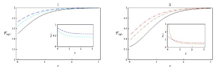
Figure 4.1: Optimal fidelity of teleportation $\mathcal{F}_{opt}$, as a function of the squeezing parameter $r$, with $\phi=\pi$ for truncated Gaussian resources. In Panel I, we report the fidelity for the teleportation of input coherent states $|\,\beta\,\rangle$ using different two-mode entangled resources: (a) Gaussian two-mode squeezed state (full line); (b) squeezed Bell-like state (dashed line); (c) squeezed symmetric superposition of Fock states (long-dashed line). In Panel II, we report the fidelity for the teleportation of input single-photon Fock state $|\,1\,\rangle$ using different two-mode entangled resources: (a) Gaussian two-mode squeezed state (full line); (b) squeezed Bell-like state (dot-dashed line); (c) squeezed symmetric superposition of Fock states (double-dot-dashed line). In plot I the value of $\beta$ is arbitrary. The insets in both Panels give the maximal values of the parameter $s=\tilde{s}$ as a function of $r$ for a given entangled resource and fixed input state. The plot styles are chosen as specified above.

4.1.3 Entanglement, non-Gaussian character and Gaussian affinity for truncated Gaussians

In section 3.4, to understand the properties of the optimized teleportation resources, we have investigated three quantities: the von Neumann entropy $E_{vN}$ (eq. (3.24)) as a measure of the amount of entanglement in the resource; the non-Gaussianity $d_{nG}$ (eq. (3.25)), to provide a measure of the non-Gaussian character of the resource; and the squeezed vacuum affinity $\mathcal{G}$ (eq. (3.26)), in order to determine the degree of resemblance of the resource to the closest two-mode squeezed vacuum.

In fig. (4.2), we plot the entanglement measure for pure states $E_{vN}$ (eq. (3.24)); for the optimized non-Gaussian entangled resources above mentioned and used as teleportation resources, and for the two-mode squeezed vacuum. All the curves exhibit very similar behaviors. At fixed $r$, and for a given input state, the optimized SSSF state is the most entangled; the optimal resource for the teleportation of a single-photon Fock state having more entanglement than the resource for the optimal teleportation of a coherent state; this can lead to the conclusion that the non-Gaussian input requires more entanglement for optimal teleportation.

The behavior of the von Neumann entropies across different classes of resources is in agreement with the behavior of the optimal fidelities. In fact, for a given input state, a non-Gaussian resource with a higher teleportation fidelity (in fig. (4.1)) is associated with a higher amount of entanglement content for any $r$.

It is not remarkable that the Gaussian truncation (see eq. (4.1)) to higher order ($n=2$, optimal SSSF state)) shows a higher von Neumann entropy that the Gaussian truncation to lower order ($n=1$, optimal Bell-like resource). We can only speculate that a higher-order ($n>2$) truncation will have a higher von Neumann entropy for the same squeezing $r$. What seems remarkable, is that for the same squeezing parameter $r$, the un-truncated Gaussian has the lowest von Neumann entropy. Before beginning to speculate as to the truncation order in which the von Neumann entropy begins to diminish, let us think again about what is meant by Gaussian ”truncation”. Inspecting eq. (4.1); and on seeing the squeezing $-(r+s)$ performed on the resource to be ”truncated”, we can only conclude that to be ”fair” to the Gaussian resource, the optimal non-Gaussian resources used here (defined by their parameters $-r$ and $-\tilde{s}$, see eq. (4.5)) should be compared to a two-mode squeezed vacuum of squeezing $-(r+\tilde{s})$ instead. We rephrase our claim: ”truncating” the Gaussian resource  raises the entanglement of the resource: from that associated to a squeezing $r$ for a two-mode squeezed vacuum, to that associated to a squeezing $r+s^{\prime}$ for the same state. This added squeezing $s^{\prime}$ is a free superposition parameter to be chosen. From inspection of figs. (4.1) and (4.2): for the optimal resources we have considered the added squeezing $\tilde{s}$ (and its effect on entanglement) is of the order of magnitude of the squeezing $r$ (and its associated levels of entanglement).

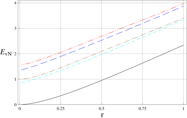
Figure 4.2: Plot of the von Neumann entropy $E_{vN}$ as a function of $r$, with $s=\tilde{s}$ (see the insets in fig. 4.1), corresponding to the following entangled resources: squeezed symmetric superposition of Fock states, squeezed Bell-like states, and two-mode squeezed vacuum states, optimized for the teleportation of coherent state inputs, and the single-photon Fock state input. The plot styles are chosen as specified in fig. (4.1).

Next, we examine the behavior of the non-Gaussianity $d_{nG}$, a measure of the difference between the resource and a reference Gaussian state with the same first and second-order moments. In fig. (4.3), panel I: we plot $d_{nG}$ (eq. (3.25)) for the SSSF resources and the squeezed Bell-like resources, optimized both for the coherent inputs and for the single-photon Fock input. The difference in non-Gaussianity between the coherent input and Fock input cases for $r=0$ is remarkable. While the resources are entangled even with no squeezing; it seems that optimization for very low $r$ is just an attempt at (nearly) classical teleportation. The behavior of the pairs of $d_{nG}$ curves corresponding to the teleportation of the same input states (either coherent or Fock) for different resources (SSSF and Bell-like) is very similar; a pair of curves (the Fock state input’s) crosses at a certain value of $r$. All the curves tend to the same small asymptotic value of $d_{nG}$ for very large $r$, as expected. Therefore, according to this measure of non-Gaussianity: the non-Gaussian resource with a higher teleportation fidelity (the SSSF state) does not exhibit a significantly higher non-Gaussian character for any $r$.

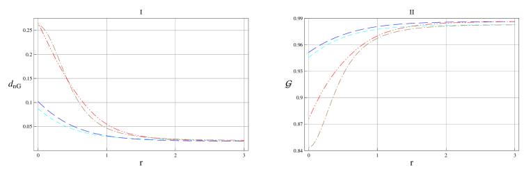
Figure 4.3: Plot of the non-Gaussianity $d_{nG}$ (panel I) and of the squeezed vacuum affinity $\mathcal{G}$ (panel II) as a function of $r$, with $s=\tilde{s}$ (see the insets in fig. (4.1)), corresponding to the following entangled resources: squeezed symmetric superposition of Fock states, and squeezed Bell-like states, optimized for the teleportation of input coherent states and the single-photon Fock input state. The plot styles are chosen as specified in fig. (4.1).

Lastly, we turn our attention to the Gaussian resource affinity $\mathcal{G}$ (eq. (3.26)), given as a measure of the maximum similarity of the resource to an ideal two-mode squeezed vacuum. In fig. (4.3) panel II: we plot $\mathcal{G}$ for the SSSF and squeezed Bell-like resources, as always optimized for the teleportation of given input states. We can see a mirror of the behaviors of $d_{nG}$ for $r\rightarrow\,0$. All the curves have a high asymptotic value of $\mathcal{G}$ for large $r$, a fact consistent with the results for non-Gaussianity $d_{nG}$. Most importantly: For the same class of input state (either coherent or Fock), the optimized SSSF state possesses a greater squeezed vacuum affinity than that of the squeezed Bell-like state, for any $r$. This result is in complete agreement with the behaviors of the corresponding optimal teleportation fidelities and von Neumann entropies studied before.

Comparing the behaviors associated with resources optimized for the efficient teleportation of the same input states, we conclude that the following hierarchy can be established: The enhancement of the teleportation fidelity corresponds to an enhancement of the entanglement content, and to an enhancement of squeezed vacuum affinity. The measure of non-Gaussianity $d_{nG}$ seems not to have a place in this hierarchy. This result shows that such a measure must be used and interpreted with attention, case by case.

Further conclusions can be drawn from the above discussion: The squeezed truncated Gaussian resource, with truncation at $n=2$ (SSSF state, with a four-photon term) is an entangled non-Gaussian resource suitable for sculpturing and optimization as regards CV quantum teleportation. We argue that this result can be generalized to higher orders ($n>2$) in expansions of the two-mode squeezed vacuum.

Therefore, we conjecture that in general, efficient entangled non-Gaussian resources for CV quantum teleportation should be characterized by a suitable balance between the entanglement content and the degree of affinity to squeezed vacuum states.

4.2 Squeezed cat-like states

In this section, we define and use as teleportation resources a special class of two-mode squeezed superposition. This time, instead of using (solely) Fock states for the superposition we use coherent states. Namely the vacuum (which is a coherent state) and an arbitrary separable coherent state with the same displacement on both it’s modes. These can be thought of as more feasible and more amenable to manipulation than the superpositions made of the highly nonclassical Fock states. We remark that the engineering of states of such a form is made possible, in principle, by the recent successful experimental realization of their single-mode equivalents [18].

4.2.1 Definition: squeezed cat-like states

The squeezed cat-like state is given by the two-mode squeezed superposition of coherent states

$$|\,\psi\,\rangle_{SC}=\,\mathcal{N}\>\widehat{S}_{AB}(\zeta)\;\left\{\cos(\delta)\,|\,0\,,\,0\,\rangle_{AB}\>+\>e^{\,i\,\theta}\,\sin(\delta)\,|\,\gamma\,,\,\gamma\,\rangle_{AB}\right\}$$ (4.6)

where the normalization factor is $\mathcal{N}=\left(1\,+\,e^{\,-|\,\gamma\,|^{2}}\>\sin(2\,\delta)\>\cos(\theta)\right)^{-1/2}$. Without the two-mode squeezing, eq. 4.6 becomes an entangled Schrödinger Cat state. The one and two-mode cat states have been proposed as qubits and as entangled resources (respectively) for quantum information processing; together with an universal set of operations for this purpose [30].

The state in eq. (4.6) can be regarded as the substitution of a coherent state $|\,\gamma\,,\,\gamma\,\rangle_{AB}$ for the two-photon $|\,1\,,\,1\,\rangle_{AB}$, in the squeezed Bell-like state of eq. (3.13). Thus producing a more classical two-mode squeezed superposition that is non-Gaussian and entangled even for zero squeezing $r$.

Following the same reasoning used to calculate the characteristic function of the SSSF state and using mostly the same identities, plus the composition law for displacement operators (eq. (1.18)), the characteristic function for squeezed cat-like resource of eq. (4.6) can be easily calculated. For $\theta=0$ it is given by

$$\chi_{SC}(\xi_{A};\>\xi_{B})= \,\mathcal{N}^{\,2}\>e^{\,-\frac{1}{2}(|\,\xi_{A}^{\prime}\,|^{2}\,+\,|\,\xi_{B}^{\prime}\,|^{2})}$$

$$\times\,((\cos(\delta))^{2}\,+\,\frac{\sin(2\,\delta)}{2}\,e^{\,-|\,\gamma\,|^{2}}\,\left(e^{\,\gamma^{*}(\xi_{A}^{\prime}\,+\,\xi_{B}^{\prime})}\,+\,e^{\,-\gamma\left(\xi_{A}^{\prime}\,+\,\xi_{B}^{\prime}\right)^{\,*}}\right)$$

$$+\,(\sin(\delta))^{2}\,e^{\,2\,i\,\mathrm{Im}[\gamma^{*}(\xi_{A}^{\prime}\,+\,\xi_{B}^{\prime})]})$$ (4.7)

where $\xi_{A}^{\prime}$ and $\xi_{B}^{\prime}$ are related to $\xi_{A}$ and $\xi_{B}$ by the Bogoliubov transformation for the displacement operator arguments in eq. (1.46).

4.2.2 Optimized teleportation fidelities with cat-like states

We can compute analytically the fidelity of teleportation using squeezed cat-like states as entangled resources, limiting the analysis, for simplicity’s sake, to the teleportation of coherent state inputs (eq. (3.15)). The maximization procedure is discussed in appendix A, including the analytical expression for the fidelity. At fixed squeezing $r$, the fidelity in eq. (A.5) may be optimized over the real amplitude $|\,\gamma\,|$ (the only free parameter remaining). Therefore;

$$\mathcal{F}_{opt}(r)\,=\,\max_{\,|\,\gamma\,|\,}\>\mathcal{F}_{SC}\left(\,r,\,|\,\gamma\,|\,\right)$$ (4.8)

In fig. (4.4), we show the behavior of $\mathcal{F}_{opt}$ as a function of $r$ for coherent state inputs, using an optimized squeezed cat-like state as a teleportation resource. For comparison, the optimal fidelities corresponding to the teleportation with Gaussian squeezed state resources and with optimized, squeezed Bell-like states are plotted. The optimized squeezed cat-like resources, for all $r$, yield a significant improvement of the fidelity with respect to the two-mode squeezed vacuum, but are less efficient than squeezed Bell-like resources; all three curves show the same behavior, including the same asymptotic behavior. The high value of $\tilde{\gamma}$ for $r=0$ is a result of the optimization trying to increase the usable entanglement that is present in a two-mode Schrödinger cat state. For much larger squeezing, the optimal amplitude $\tilde{\gamma}$ tends to a smaller, asymptotic value; this behavior is consistent with the behavior of the resource, which eventually becomes an EPR state, for $r\rightarrow\infty$.

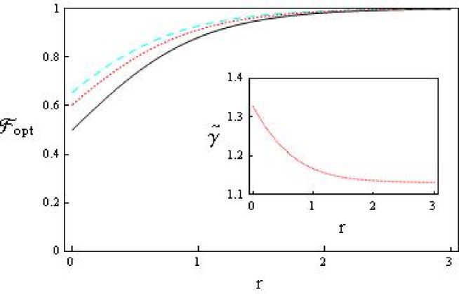
Figure 4.4: Optimal fidelity of teleportation $\mathcal{F}_{opt}$, as a function of the squeezing parameter $r$, with $\phi=\pi$, using squeezed cat-like resources. The fidelity corresponds to the teleportation of input coherent states with a squeezed cat-like state as entangled resource (dotted line). For comparison, we plot the fidelities obtained with a squeezed vacuum resource (full line) and with a squeezed Bell-like resource (dashed line). The inset gives the optimal value of the parameter $|\,\gamma\,|=|\,\tilde{\gamma}\,|$ as a function of $r$.

4.2.3 Entanglement, non-Gaussian character and Gaussian affinity for cat-like states

The behavior of the teleportation fidelity for the optimized, squeezed cat-like resource in fig. (4.4) is in agreement with the behaviors of its von Neumann entropy (eq. (3.24)), non-Gaussianity (eq. (3.25)), and squeezed vacuum affinity (eq. (3.26)). We report these in fig. (4.5) and fig. (4.6), panel I and panel II, respectively.

The optimized squeezed cat-like resource is less entangled, less non-Gaussian (according to the $d_{nG}$ measure), and less affine to the squeezed vacuum than the optimized squeezed Bell-like state. The entanglement as measured by the von Neumann entropy is higher for the cat-like resource than for a Gaussian, but lower than that for a Bell-like state for all values of $r$. The optimized squeezed cat-like resource exhibits a markedly lower value of $\mathcal{G}$ in comparison with the truncated Gaussian resources. This can be seen by comparing fig. (4.6), panel II with the corresponding plots shown in fig. (4.3), panel II; in fact, $\mathcal{G}$ seems to have an asymptote at value $71\%$ (approached from below).

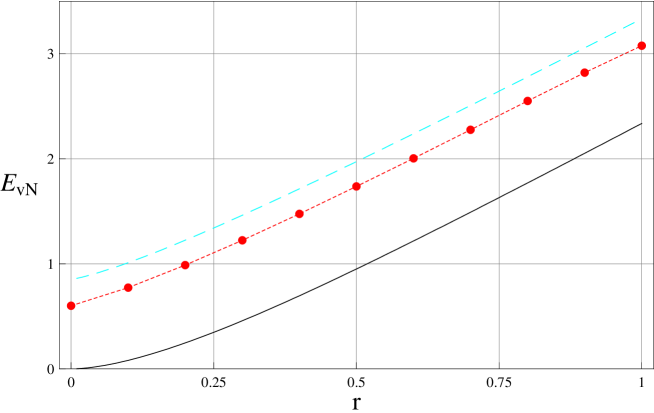
Figure 4.5: Behavior of the von Neumann entropy $E_{vN}$ as a function of $r$, with $|\,\gamma\,|=\tilde{\gamma}$ (see the inset in fig. (4.4)) for the optimized squeezed cat-like state (dotted line). For comparison, we also plot the quantities $E_{vN}$ corresponding to a two-mode squeezed vacuum (full line), and to a squeezed Bell-like state (dashed line).

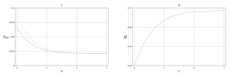
Figure 4.6: Behavior of the non-Gaussianity $d_{nG}$ (panel I) and of the squeezed vacuum affinity $\mathcal{G}$ (panel II) as a function of $r$, with $|\,\gamma\,|=\tilde{\gamma}$ (see the inset in fig. (4.4)) for the optimized squeezed cat-like state (dotted line). For comparison, in panel I we plot $d_{nG}$ for the optimized squeezed Bell-like state (dashed line).

Chapter 5 Teleportation with noisy non-Gaussian resources

In chapter 3, we defined the squeezed Bell-like states (eq. (3.13)); a class of states that include all the other non-Gaussian resources studied in that chapter, as well as the Gaussian two-mode squeezed vacuum. We optimized the Squeezed Bell-like state for the teleportation of some inputs and compared them for their properties of entanglement, non-Gaussianity and Gaussian resource affinity with the other resource states studied in that chapter. In chapter 4, we introduced the squeezed cat-like states [37] (eq. (4.6)) by substituting a coherent state term for the Fock state term in the superposition making up a Bell-like state, with the intention of creating a more feasible [18], more resilient [19] (to decoherence) resource.

In this chapter, we extend the analysis performed in chapters 3 and 4 to the realistic case of optimized, squeezed Bell-like and squeezed cat-like resources prepared or propagated in the presence of thermal noise (see section 2.4), for the teleportation of coherent state inputs [36, 37]. For comparison purposes we perform the same analysis for Gaussian two-mode squeezed vacuum states, also prepared in the presence of thermal noise.

We analyze the behavior of inseparability parameters developed for general CV contexts [41, 42], for Bell-like and Gaussian resource states. For a practical measure of the disappearance (or appearance) of entanglement of teleportation, we consider the level of noise at which the resource passes the classical teleportation threshold [39, 40] of $1/2$, for a fixed squeezing. This last analysis is performed for both the squeezed Bell-like resource and the squeezed cat-like resource, with the squeezed vacuum put in for comparison purposes.

5.1 Fidelity of teleportation with mixed, noisy non-Gaussian resources

The presence of thermal noise in the preparation of the resource states can be modelled by superimposing a pure resource state on thermal states (see section 2.4) in modes $A$ and $B$ of the resource. The characteristic function of such a preparation (see eq. (2.41)) is given by

$$\chi_{AB}^{(th)}(\xi_{A},\xi_{B})\,=\,e^{-n_{th,A}|\xi_{A}|^{2}-n_{th,B}|\xi_{B}|^{2}}\,\chi_{AB}(\xi_{A},\xi_{B})$$ (5.1)

where $n_{th,A},n_{th,B}$ are the mean photon numbers; thermal parameters associated with the modes $A$ and $B$.

The state of eq. (5.1) is mixed for $n_{th,A},n_{th,B}\neq\,0$. $\chi_{AB}$ is the characteristic function for the pure resource state thus superimposed over thermal states. We substitute in eq. (5.1) the characteristic functions of either the squeezed Bell-like state (eq. (3.14)); the squeezed cat-like resource (eq. (4.7)) or the two-mode squeezed vacuum (eq. (1.58)) to produce the respective ”noisy” teleportation resources.

Substituting the resource of eq. (5.1) in eq. (2.26) with a coherent state input (eq. (3.15)) and $g_{x}=g_{p}=1$; we obtain the output for CV teleportation with a noisy resource. From the output state, it is straightforward to calculate the analytic expression for teleportation fidelity as a function of the adequate superposition parameters: $\delta$ for the squeezed Bell-like state and $|\,\gamma\,|$ for the squeezed cat-like states. The squeezing parameter $r$ is fixed and $\phi=\pi$ in keeping with convention. Likewise are fixed the thermal parameters $n_{th,A}$ and $n_{th,B}$. The analytic expressions of the fidelities for the noisy non-Gaussian resources in the teleportation of coherent states; squeezed Bell-like ($\mathcal{F}_{SB}^{\,(th)\,}(\,r\,,\,n_{th,A}\,,\,n_{th,B}\,,\,\delta\,)$) and squeezed cat-like ($\mathcal{F}_{SC}^{(th)}(\,r\,,\,n_{th,A}\,,\,n_{th,B}\,,\,|\,\gamma\,|\,)$) and an initial analysis of the optimization procedure performed on the aforementioned fidelities are reported in appendix A.

For example, for the mixed squeezed Bell-like state teleporting a coherent state, the fidelity is optimized over $\delta$, leaving other parameters fixed;

$$\mathcal{F}_{opt}(\,r\,,\,n_{th,A}\,,\,n_{th,A}\,)\,=\,\max_{\delta}\;\mathcal{F}_{SB}^{\,(th)\,}(\,r\,,\,n_{th,A}\,,\,n_{th,B}\,,\,\delta)\;,$$ (5.2)

The optimization yields an optimal angle $\delta_{max}^{(c,th)}$ that has a form not too dissimilar to that for ideal teleportation (eq. (3.21));

$$\delta_{max}^{(\,c\,,\,th\,)}\,=\,\frac{1}{2}\;\arctan\left(\,1\,+\,\frac{e^{\,-\,2\,r}}{1\,+\,n_{th,A}\,+\,n_{th,B}}\right)$$ (5.3)

which reduces to the pure state case if the thermal parameters $n_{th,A}=n_{th,B}=0$. When this angle is substituted in the expression for the fidelity (eq. (A.1)) gives the optimal fidelity for a mixed Bell-like resource.

In the case of mixed squeezed cat-like states, at given thermal numbers $n_{th,A}$, $n_{th,B}$ and fixed squeezing parameter $r$, the optimal fidelity is defined as

$$\mathcal{F}_{opt}(\,r\,,\,n_{th,A}\,,\,n_{th,B}\,)\,=\,\max_{|\,\gamma\,|}\;\mathcal{F}_{SC}^{\,(th)}(\,r\,,\,n_{th,A}\,,\,n_{th,B},|\,\gamma\,|)\;$$ (5.4)

where the maximization is performed numerically for fixed values of $r$ and $n_{th}=n_{th,A}=n_{th,B}$.

In fig. (5.1); we plot the optimal fidelities for the mixed non-Gaussian resources as a function of squeezing for various choices of the thermal parameters $n_{th,A}=n_{th,B}=n_{th}$. Along, we plot the fidelities for a Gaussian two-mode squeezed vacuum, used as a benchmark. We observe that, as expected, the fidelity decreases for increasing $n_{th}$: the thermal noise sensibly reduces the success probability of teleportation, as it reduces the entanglement content of the resources. We can also observe that for similar noise $n_{th}$ the asymptote for large $r$ is the same for all resources: the asymptote indicates the convergence of all resources to a mixed two-mode squeezed vacuum at high squeezing, with the ”mixedness” putting an upper bound on teleportation fidelity even for this nearly ideal resource.

An important observation is that in our plot, for the chosen realistic values for $n_{th}$; the fidelity associated with both non-Gaussian mixed resources never drops below the threshold of classical teleportation [39] with maximal fidelity $\mathcal{F}_{cls}^{max}=1/2$. The ability of the resource to keep the fidelity above this benchmark value of $1/2$ will be made a practical measure of resilience in presence of noise; in the next section.

At fixed squeezing and thermal parameters, the non-Gaussian resources always perform better than the Gaussian two-mode squeezed vacuum. Furthermore, mixed squeezed Bell-like states have a higher performance than the mixed squeezed cat-like states. We remark that the better performance of the mixed Bell-like states over the mixed cat-like states has been demonstrated for this simple analysis of environmental noise. Other sources of noise (and decoherence) have not been studied.

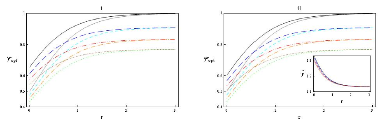
Figure 5.1: Optimal fidelity $\mathcal{F}_{opt}$, associated with the teleportation of input coherent states with mixed squeezed Bell-like resources (panel I) and mixed squeezed cat-like resources (panel II), as a function of the squeezing $r$, for several choices of the thermal parameters $n_{th,A}=n_{th,B}=n_{th}$. The curves representing the fidelities associated with mixed non-Gaussian entangled resources are plotted with the following plot style: $n_{th}=0$ (full black line), $n_{th}=0.05$ (long-dashed line), $n_{th}=0.10$ (double-dot dashed line), and $n_{th}=0.15$ (dotted line). For comparison, in both panels, we also plot the fidelities associated to the mixed squeezed vacuum entangled resources, with $n_{th}=0$ (full gray line), $n_{th}=0.05$ (dashed line), $n_{th}=0.10$ (dot-dashed line), and $n_{th}=0.15$ (long-dotted line). The inset in panel II gives the maximal value of the parameter $|\,\gamma\,|=\tilde{\gamma}$ as a function of $r$, with $n_{th}=0,\,0.05,\,0.1,\,0.15$ (same plot style as for the fidelities).

We have chosen the mixed Gaussian state to be a reference resource (see subsection 3.3.2) for the evaluation of the performance of the squeezed Bell-like state in teleportation. To develop this relationship between resources further; we define the relative fidelity (see eq. (3.23)) given for mixed squeezed Bell-like state and referring to the mixed Gaussian state

$$\Delta\mathcal{F}^{(c)}_{opt}(r,n_{th})\,=\,\frac{\mathcal{F}^{(c)}(r,n_{th},n_{th},\delta_{max}^{(c,th)})-\mathcal{F}^{(c)}(r,n_{th},n_{th},0)}{\mathcal{F}^{(c)}(r,n_{th},n_{th},0)}$$ (5.5)

where $\mathcal{F}^{(c)}(r,n_{th},n_{th},0)$ is the fidelity for the mixed Gaussian resource and $\mathcal{F}^{(c)}(r,n_{th},n_{th},\delta_{max}^{(c,th)})$ is the fidelity for the optimized noisy Bell-like resource (eq. (A.1)).

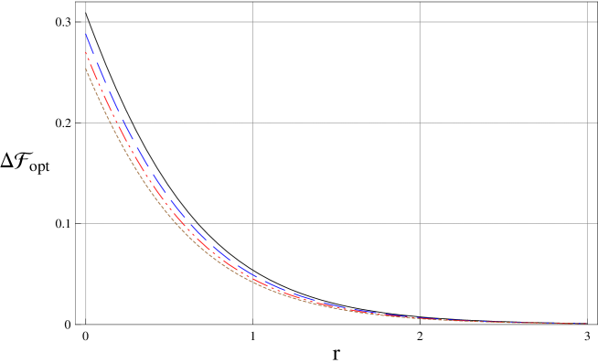
Figure 5.2: Relative fidelity for mixed Bell-like resources with respect to mixed Gaussian resources for coherent state inputs; $\Delta\mathcal{F}^{(c)}_{opt}(r,n_{th})$ as a function of the squeezing $r$, for several choices of the thermal parameter $n_{th,A}=n_{th,B}=n_{th}$: $n_{th}=0$ (full black line), $n_{th}=0.05$ (long-dashed line), $n_{th}=0.10$ (double-dot dashed line), $n_{th}=0.15$ (dotted line).

In fig. (5.2) we show the behavior of $\Delta\mathcal{F}^{(c)}_{opt}(r,n_{th})$ as a function of $r$. We see that the percent gain in the fidelity for $n_{th}=0$ essentially coincides with the one defined in the absence of thermal noise (fig. (3.6)). It is also evident that for ever increasing $n_{th}$, both the resources will converge asymptotically to $\Delta\mathcal{F}^{(c)}_{opt}(r,n_{th})=0$. This signals a similar and very poor performance in teleportation for both resources; corresponding to a separable, mixed, thermal state of two-modes.

We have shown that the mixed non-Gaussian resources; although with reduced fidelity with respect to the ideal resources, are better choices than the mixed Gaussian two-mode squeezed resource. Both the non-Gaussian resources studied here also provide acceptable (always better than the Gaussian) values of the fidelity for technically feasible squeezing $r$ and realistic values of thermal mean photon number $n_{th}$.

5.2 Inseparability criteria and classical teleportation: Bell-like, cat-like and Gaussian resources

In ref. [24] it has been shown that the entanglement, that is a fundamental requirement for the efficient implementation of nonclassical teleportation protocols, is remarkably enhanced in the Bell-like state when compared to the Gaussian squeezed vacuum. Even though the pure squeezed Bell-like state has entanglement for $r=0$; the introduction of noise (and of a mixed nature) induces a lowering of the amount of entanglement in the Bell-like state. It is then necessary to check that, for fixed values of the thermal parameter $n_{th}$, a sufficient amount of entanglement still survives and is useful for teleportation, above a classical threshold value.

In order to avoid the not-yet-solved problem of computing the amount of entanglement by means of a measure appropriate for all mixed states; we can exploit an inseparability criterion, based on the condition of positivity under partial transposition (PPT criterion) [86, 87, 88, 41, 42]. For the purpose of knowing where (for which values of $r$ and $n_{th}$) a state becomes inseparable and possibly useful for quantum teleportation, we assume this criterion to be just as useful as a proper entanglement measure.

In our case, the PPT criterion can be expressed through an inequality for a inseparability parameter $\Delta$ involving only second order statistical moments:

$$\Delta\,=\,\langle\>\hat{a}_{A}^{{\dagger}}\,\hat{a}_{A}\>\rangle\>\langle\>\hat{a}_{B}^{{\dagger}}\,\hat{a}_{B}\>\rangle\;-\;|\,\langle\>\hat{a}_{A}\,\hat{a}_{B}\>\rangle\,|^{2}\,<\,0$$ (5.6)

which are straightforward to calculate, as the characteristic function of a quantum state is the generating function for the statistical moments of the state (see eq.(1.57)).

Let us recall that the inequality in eq. (5.6) is a sufficient inseparability condition for non-Gaussian states, being necessary and sufficient for Gaussian states. In fig. (5.3); we plot the behavior of $\Delta$ as a function of $r$ for several choices of the thermal parameters $n_{th,A}=n_{th,B}=n_{th}$, both for the mixed squeezed Bell-like state and for the mixed squeezed vacuum state.

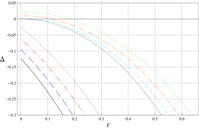
Figure 5.3: Behavior of the inseparability parameter $\Delta$ as a function of the squeezing $r$, for several choices of the thermal parameters $n_{th,A}=n_{th,B}=n_{th}$. Plots are for the mixed squeezed Bell-like state, with $n_{th}=0$ (full black line), $n_{th}=0.05$ (long-dashed line), $n_{th}=0.10$ (double-dot dashed line), $n_{th}=0.15$ (dotted line); and for the noisy squeezed vacuum state, with $n_{th}=0$ (full gray line), $n_{th}=0.05$ (dashed line), $n_{th}=0.10$ (dot-dashed line), $n_{th}=0.15$ (long-dotted line).

Recall again that the pure Bell-like state is already entangled for $r=0$ and $\delta\neq\,0,\pi/2$ (see fig. (3.8)). For realistic values of $n_{th}$ ($0$ to $0.15$) we see the mixed Bell-like state exhibiting entanglement. On the other hand, for $n_{th}>\,0$, the mixed squeezed vacuum state has $\Delta\geq 0$ at sufficiently low values of $r$; i.e. it becomes separable. Specifically, for the mixed Gaussian state the threshold value $n_{th}^{(sep)}$ for separability is $n_{th}^{(sep)}(r)=\frac{1\,-\,e^{\,-\,2\,r}}{2}$.

Though we have defined no measure for entanglement, and in particular, no measure of entanglement useful for CV teleportation; we have in the two-mode squeezed vacuum a practical reference resource,with a ”maximum classical fidelity” $\mathcal{F}_{cls}^{max}=0.5$ that is widely accepted as a practical threshold [39, 40] for CV teleportation of coherent states. We can assume for practical purposes that quantum teleportation becomes impractical when thermal noise causes fidelity to go under this value.

Therefore, for a resource that teleports coherent states, we define the classical threshold value of the thermal parameter $n_{th}^{(cls)}(r)$: At a fixed $r$ and for $n_{th}=n_{th}^{(cls)}(r)$, the optimal fidelity $\mathcal{F}_{opt}=\mathcal{F}_{cls}^{max}=1/2$. The optimal fidelity goes above the $1/2$ threshold in a smooth manner for $n_{th}<n_{th}^{(cls)}(r)$, and goes smoothly below the threshold $1/2$ for $n_{th}>n_{th}^{(cls)}(r)$. For this it is assumed (and found for the resources used here) that the optimal fidelity is an analytical function of $r$ and $n_{th}$.

In fig. 5.4 we plot $n_{th}^{(cls)}$ as a function of $r$ for the optimized, mixed squeezed Bell-like resource, the optimized mixed squeezed cat-like resource and the mixed squeezed Gaussian resource, shown as a reference.

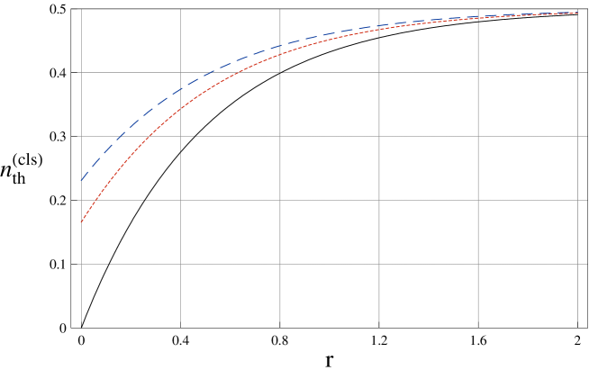
Figure 5.4: Behavior of the classical threshold value $n_{th}^{(cls)}$ of the thermal parameter as a function of $r$, for mixed squeezed Bell-like resources (dashed line), mixed squeezed cat-like resources (dotted line), and mixed squeezed vacuum, shown as a reference (full line).

We see that the threshold value $n_{th}^{(cls)}$ associated to non-Gaussian resources is larger than that associated to Gaussian ones, and in any case sensibly larger than the reasonable realistic values ($n_{th}\leq\,0.15$) we have considered. Even for $r=0$ the non-Gaussian resources, always under realistic conditions, show entanglement allowing teleportation fidelities greater than the classical threshold. On the contrary, the fidelity associated with the mixed squeezed vacuum state, at low values of $r$ falls below the classical threshold, unless optimization is performed on the local degrees of squeezing, without modifying the Braunstein-Kimble protocol [89].

It is remarkable that the squeezed Bell-like state has a consistently higher value of $n_{th}^{(cls)}$ than the squeezed cat-like state. Taking this result at face value, it can be said that the Bell-like state is more resilient in noisy environments than the squeezed cat-like state, at equal $r$. Note lastly that for mixed squeezed vacuums, $n_{th}^{(cls)}(r)$ coincides with the threshold value for separability, that is $n_{th}^{(cls)}(r)=n_{th}^{(sep)}(r)=\frac{1\,-\,e^{\,-\,2\,r}}{2}$.

Compare fig. (5.2) with fig. (5.4) for the squeezed Bell-like resource. In the former, increasing $n_{th}$ makes for a marked decrease in $\Delta\mathcal{F}^{(c)}_{opt}(r,n_{th})$ for all $r$. In the latter, the asymptotic limit of $n_{th}^{(cls)}(r)$, for both Gaussian and non-Gaussian resources is the same. Therefore, we have a value of $n_{th}\approx\,0.5$ beyond which no reasonable amount of two-mode squeezing $r$ will avail to produce a useful  resource for quantum teleportation out of either a Gaussian resource or a Bell-like resource of any kind. Fortunately, this value of $n_{th}$ is considered huge for a realistic experimental setting.

Chapter 6 Conclusions

We have developed a Wigner’s characteristic function based formalism that allows for the intuitive representation of the formalism for CV quantum teleportation for any combination of resource and input states for which these characteristic functions exist. The formalism is not confined to the original protocol; furthermore, it is possible to introduce further and more complicated steps to the protocol; measurements different from homodyne detection of EPR states and the mixing in of external modes representing noise, photon addition and photon subtraction. We have further shown that an analysis of the expression for the teleportation fidelity makes for a trivial derivation of results for resource states that are simple mixtures of pure states. The characteristic function formalism, as it stands, can easily accommodate most of the conceivable operations and measurements involved in CV teleportation, together with simple modifications to the protocol. It is then, possible, to use characteristic functions to ”model” other quantum information protocols in a convenient manner.

We have presented a thorough comparison, with regard to the performance in continuous-variable quantum teleportation, between standard Gaussian, wholly non-Gaussian (two-mode squeezed Fock state) and degaussified resources (such as photon-added and photon-subtracted squeezed states) and a new type of sculptured resource that interpolates between these states and can be optimized because it depends on an extra, relative-phase, independent free parameter in addition to squeezing. These sculptured non-Gaussian resources we have named squeezed Bell-like states: They hybridize discrete single-photon pumping, coherent superposition of Bell two-qubit eigenstates, and CV squeezing; thus including the above mentioned resources as ”special cases”. The maximization of the teleportation fidelity (an analytical expression which is valid for a given input state) is made with respect to the free parameter. Therefore we have produced a fidelity that is optimal for the class of Bell-like states including, most importantly, all the ”special case” resources. Understanding the enhancement yielded by sculptured squeezed Bell-like resources in teleportation success is possible when certain properties of the resources used are studied and compared jointly. The optimized squeezed Bell-like states are those states that are as close as possible to the simultaneous maximization of entanglement, non-Gaussianity, and affinity to the two-mode squeezed vacuum.

We have proposed a method for the experimental generation of squeezed Bell-like states using a cascading setup of second and third-order non-linear crystals. Given the nature of the squeezed Bell-like states, this method is to be additionally regarded as an alternative method for the generation of degaussified resources.

We have further generalized the Bell-like states by including an additional four-photon term in the superposition, producing squeezed symmetric superpositions of Fock (SSSF) states. These resources, with an added dimension for sculpturing, can be utilized to an optimal fidelity of teleportation that is a notable improvement even over the optimal Bell-like state fidelity. We have considered the Bell-like states as first-order truncations of a $r+s$ squeezing Gaussian state where $r$ is genuine two-mode squeezing and $s$ depends on the character of the Bell-like state; we found, remarkably, that the optimal SSSF resource is to be formulated as the second-order truncation of the same $r+s$ squeezing Gaussian states. We have argued that a Gaussian ”truncation” should be compared to the $r+s$ squeezing Gaussian instead of the $r$ squeezing Gaussian. The analysis of the properties for these states, the Bell-like and the SSSF shows that the optimal teleportation resource comes close to simultaneously maximizing entanglement and affinity to the two-mode squeezed vacuum. Not so for the non-Gaussianity.

We have introduced, and optimized for teleportation a class of two-mode squeezed cat-like states; superpositions of coherent states that are then two-mode squeezed. These states have been optimized for teleportation over their coherent amplitudes, obtaining performances and entanglement values that are higher than those for Gaussian resources; but lower than those for Bell-like states. These entangled states are interesting because of their, in principle, greater feasibility [18] in comparison with Bell-like and SSSF states, which involve superpositions of few-photon Fock states.

Given the above results, we state that the optimization of the ideal CV teleportation protocol with non-Gaussian resources necessitates only the formulation of more general and more complicated non-Gaussian resources. The only difficulty to be incurred in the generalization of non-Gaussian resources lies is in the analytic calculation of the fidelities for the purpose of optimization of the same.

Further optimization is in principle possible with respect to the local parts of the resource states, in analogy to the case of standard Gaussian resources [89]. One could think of extending the sculpturing to the entire basis of Bell states, to generate entangled non-Gaussian resources that can never be reduced to proper truncations of Gaussian squeezed resources. Such fully sculptured resources might allow for the further enhancement of the teleportation success due to the presence of a larger number of experimentally adjustable free parameters in addition to squeezing. Fully sculptured states could be applied to hybrid schemes of teleportation combining continuous-variable inputs with discrete-variable resources and viceversa. In this framework, a particularly appealing line of research would be to look for modified schemes of teleportation beyond the standard Braunstein-Kimble protocol, to be realized by generalized measurements in combination with state-control enhancing unitary operations.

We have studied the efficiency of CV teleportation of input coherent states using, as resources, squeezed Bell-like and squeezed cat-like states, prepared, superimposed over initial thermal states that represent thermal noise. Thus we have defined general non-Gaussian, realistically mixed entangled states. We have shown that, although the thermal noise strongly affects the success probability of teleportation, the resource provided by the optimized mixed extensions of the non-Gaussian squeezed Bell-like and squeezed cat-like states guarantee a sufficiently high fidelity, for realistic values of the average thermal photon number $n_{th}$ and of the squeezing $r$. A better performance is assured always, with respect to the mixed extension of the Gaussian twin beam.

We have calculated some simple expressions for the characteristic function of the teleportation output for different models of nonideal Bell measurement. The analysis of ”noisy” teleportation that we have performed can be generalized using the above mentioned results, while taking into account the decoherence induced by the propagation of the resource in noisy channels.

Finally, the present discussion could be extended to other types of quantum information tasks and processes besides teleportation. For instance, it would be interesting to investigate the comparative effects of non-Gaussian inputs and non-Gaussian resources in schemes for the generation of macroscopic and mesoscopic optomechanical entanglement [90]. A further goal will be the study of optimal teleportation with non-Gaussian resources of two-mode and multimode states [91].

Appendix A Analytic expressions of Teleportation fidelities

In this appendix we report the explicit, analytic expressions for the teleportation fidelities calculated in chapters 3 and 5. We have deemed these expressions both too cumbersome and unnecessary for the purposes of our exposition regarding the CV teleportation protocol with Non-Gaussian resources; relying instead on the plots accompanying the exposition for the graphical representation of said fidelities.

A.1 The fidelities: noisy squeezed Bell-like states with coherent state inputs

The fidelity $\mathcal{F}^{(c)}(r\,,\,n_{th,A}\,,\,n_{th,B}\,,\,\delta)$ (superposition phase $\theta=0$; squeezing angle $\phi=\pi$) for the CV teleportation of a coherent state input of arbitrary amplitude, using as a resource the mixed squeezed Bell-like state (see eq. (5.1 and eq. (3.14) reads

$$\mathcal{F}^{(c)}(\,r\,,\,n_{th,A}\,,\,n_{th,B}\,,\,\delta)\,=\,\frac{1+e^{\,2\,r}f_{th}\>+\>e^{\,4\,r}f_{th}^{2}\>+\>e^{\,2\,r}f_{th}\,\cos(2\delta)\>+\>[1\,+\,e^{\,2\,r}f_{th}]\sin(2\,\delta)}{e^{\,-2\,r}[1\,+\,e^{\,2\,r}f_{th}]^{3}}$$ (A.1)

where

$$f_{th}\equiv\,1\,+\,n_{th,A}\,+\,n_{th,B}$$ (A.2)

The fidelities for the states that are special cases of the Squeezed Bell-like state (see section 3.1) can be obtained by the substitution the appropriate values of the $\delta$ parameter in eq. (A.1) and the appropriate levels of noise $n_{th,A}$ and $n_{th,B}$. For the case in which $\delta=0$ and $n_{th,A}=n_{th,B}$=0, the fidelity equals the well-known result

$$\mathcal{F}_{TwB}(r)\,=\,\frac{1}{1\,+\,e^{\,-\,2\,r}}$$ (A.3)

holding for pure two-mode squeezed vacuum resources and coherent state inputs [39].

In the absence of thermal fields, for $n_{th,A}=n_{th,B}=0$; we have $f_{th}=1$, and the fidelity reducing to the pure resource fidelities studied in chapter 3. Notice that, in the limit of large thermal parameter, the fidelity of teleportation in eq. (A.1) is strongly suppressed and vanishes asymptotically.

A.2 The fidelities: noisy squeezed cat-like states with coherent state inputs

We report the analytical expressions for the fidelities of teleportation of input coherent states using pure and mixed squeezed cat-like states as resources. By putting, as usual, the phases $\theta=0$ and $\phi=\pi$, the fidelity for the squeezed cat-like state (eq. (4.6)) reads

$$\mathcal{F}_{SC}^{\prime}(r\,,\,\delta\,,\,\gamma)\,=\,\frac{\cos^{2}(\delta)\,+\,e^{\,\frac{(\gamma\,-\,\gamma^{*})^{2}}{1\,+\,e^{\,2\,r}}}\,\sin^{2}(\delta)\>+\>e^{\,-|\,\gamma\,|^{2}}\>(e^{\,\frac{\gamma^{2}}{1\,+\,e^{\,2\,r}}}+e^{\frac{\gamma^{*2}}{1\,+\,e^{\,2\,r}}})\sin(\delta)\>\cos(\delta)}{(1\,+\,e^{\,-2\,r})(1\,+\,e^{-|\,\gamma\,|^{2}}\sin(2\,\delta))}$$ (A.4)

It is worth noticing that for $\delta\rightarrow 0$ and/or $\gamma\rightarrow 0$, the fidelity in eq. (A.4) reduces to the well known expression of eq. (A.3). A preliminary numerical optimization procedure for eq. (A.4) allows us to fix the parameters $\arg\gamma$ and $\delta$ to the values $\arg\gamma=0$ and $\delta=\frac{\pi}{4}$, leading to the simplification of the above fidelity to the expression

$$\mathcal{F}_{SC}\left(r\,,\,|\,\gamma\,|\right)\,=\,\frac{1\,+\,e^{\,\frac{-|\,\gamma\,|^{2}}{1\,+\,e^{\,-2\,r}}}}{(1\,+\,e^{\,-2\,r})(1\,+\,e^{-|\,\gamma\,|^{2}})}$$ (A.5)

Thus, at fixed squeezing $r$ the maximization can be carried out with the real amplitude $|\,\gamma\,|$ being the only free parameter. We have $\mathcal{F}_{opt}\,=\,\max_{|\,\gamma\,|}\mathcal{F}_{SC}\,\left(r\,,\,|\,\gamma\,|\right)$. In the limit of zero squeezing ($r=0$), the value of the optimal fidelity becomes $\mathcal{F}_{opt}\,=\,[4\>(\sqrt{2}\,-\,1)]^{-1}\simeq\,0.6035$, for $|\,\gamma\,|=\ln^{1/2}(\sqrt{2}\,-\,1)^{-2}\simeq\,1.3276$.

Lastly; consider the ”noisy”, mixed squeezed cat-like resource with fixed angle $\delta=\frac{\pi}{4}$ and phases $\phi=\pi$, $\theta=0$, $\arg\gamma=0$. The fidelity $\mathcal{F}_{SC}^{(th)}(r\,,\,n_{th,1}\,,\,n_{th,2},|\,\gamma\,|)$ for the mixed squeezed cat-like state is given by

$$\mathcal{F}_{SC}^{(th)}(r\,,\,n_{th,1}\,,\,n_{th,2},|\,\gamma\,|)\,=\,\frac{1\,+\,e^{\,-|\,\gamma\,|^{2}}e^{\,\frac{|\,\gamma\,|^{2}}{(1\,+\,e^{\,2\,r}\,f_{th})}}}{e^{\,-\,2\,r}(1\,+\,e^{\,2\,r}\,f_{th})(1\,+\,e^{\,-\,|\,\gamma\,|^{2}})}$$ (A.6)

where $f_{th}$ is given by eq. (A.2).

Bibliography

- [1] F. Dell’Anno, S. De Siena, and F. Illuminati, Phys. Rep. 428, 53 (2006).
- [2] M. S. Kim, W. Son, V. Bužek, and P. L. Knight, Phys. Rev. A 65, 032323 (2002).
- [3] A. Kitagawa, M. Takeoka, M. Sasaki, and A. Chefles, Phys. Rev. A 73, 042310 (2006).
- [4] V. V. Dodonov and L. A. de Souza, J. Opt. B: Quantum Semiclass. Opt. 7, S490 (2005).
- [5] A. P. Lund, T. C. Ralph, and P. van Loock, quant-ph/0605247.
- [6] M. M. Wolf, G. Giedke, and J. I. Cirac, Phys. Rev. Lett. 96, 080502 (2006).
- [7] G. S. Agarwal and K. Tara, Phys. Rev. A 43, 492 (1991).
- [8] G. Bjork and Y. Yamamoto, Phys. Rev. A 37, 4229 (1988).
- [9] Z. Zhang and H. Fan, Phys. Lett. A 165, 14 (1992).
- [10] M. Dakna, T. Opatrný, L. Knöll, and D. G. Welsch, Phys. Rev. A 55, 3184 (1997).
- [11] M. S. Kim, E. Park, P. L. Knight, and H. Jeong, Phys. Rev. A 71, 043805 (2005).
- [12] T. Tyc and N. Korolkova, arXiv:0709.2011v1 [quant-ph].
- [13] A. Zavatta, S. Viciani, and M. Bellini, Science 306, 660 (2004).
- [14] A. I. Lvovsky and S. A. Babichev, Phys. Rev. A 66, 011801 (2002).
- [15] J. Wenger, R. Tualle-Brouri, and P. Grangier, Phys. Rev. Lett. 92, 153601 (2004).
- [16] A. Ourjoumtsev, A. Dantan, R. Tualle-Brouri, and P. Grangier, Phys. Rev. Lett. 98, 030502 (2007).
- [17] V. Parigi, A. Zavatta, M. Kim, and M. Bellini, Science 317, 1890 (2007).
- [18] A. Ourjoumtsev, H. Jeong, R. Tualle-Brouri, and P. Grangier, Nature 448, 784 (2007).
- [19] A. Serafini, S. De Siena, F. Illuminati, and M. G. A. Paris, J. Opt. B: Quantum Semiclass. Opt. 6, S591 (2004).
- [20] S. Lloyd and S. L. Braunstein, Phys. Rev. Lett. 82, 1784 (1999).
- [21] T. Opatrný, G. Kurizki, and D.-G. Welsch, Phys. Rev. A 61, 032302 (2000).
- [22] P. T. Cochrane, T. C. Ralph, and G. J. Milburn, Phys. Rev. A 65, 062306 (2002).
- [23] S. Olivares, M. G. A. Paris, and R. Bonifacio, Phys. Rev. A 67, 032314 (2003).
- [24] F. Dell’Anno, S. De Siena, L. Albano and F. Illuminati, Phys. Rev. A 76, 022301 (2007).
- [25] M. A. Nielsen and C. M. Caves, Phys Rev. A 55, 2547 (1997).
- [26] S. L. Braunstein, G.M. D’Ariano, G.J. Milburn and M. Sacchi, Phys. Rev. Lett. 84, 3486 (2000).
- [27] H. F. Hoffman, T. Ide, T. Kobayashi and A. Furusawa, Phys. Rev. A 62, 062304 (2000); ibidem arXiv:quant-ph/0110127v1 (2001), contribution to the ISQM’01 conference held August 27th to 30th 2002 in Tokyo, publ. in Proceedings of the 7th international symposium on Foundations of Quantum Mechanics in the Light of New Technology, World Scientific, 2002.
- [28] N. J. Cerf, O. Krüger, P. Navez, R. F. Werner, and M. M. Wolf, Phys. Rev. Lett. 95, 070501 (2005).
- [29] P. van Loock, W. J. Munro, K. Nemoto, T. P. Spiller, T. D. Ladd, S. L. Braunstein, and G. J. Milburn, arXiv:quant-ph/0701057.
- [30] T. C. Ralph, A. Gilchrist, G. J. Milburn, W. J. Munro, and S. Glancy, Phys. Rev. A 68, 042319 (2003).
- [31] T. P. Spiller, K. Nemoto, S. L. Braunstein, W. J. Munro, P. van Loock, and G. J. Milburn, New J. Phys. 8, 30 (2006).
- [32] H. Weyl The Theory of Groups and Quantum Mechanics, Dover Publications, Inc., New York 1950.
- [33] S. L. Braunstein and H. J. Kimble, Phys. Rev. Lett. 80, 869 (1998).
- [34] U. Leonhardt and H. Paul, Phys. Rev. A 48,No. 6,4598 (1993).
- [35] P. Marian and T. A. Marian, J. Phys. A: Math. Gen. 29, 6233 (1996).
- [36] F. Dell’Anno, S. De Siena, L. Albano and F. Illuminati, arXiv:quant-ph/0710.3259 v1.
- [37] F. Dell’Anno, S. De Siena, L. Albano and F. Illuminati, to be publ. in EPJ.
- [38] R.J. Glauber, Phys. Rev. 131, p. 2766 (1963).
- [39] S.L. Braunstein, C.A. Fuchs and H.J. Kimble, J. Mod. Opt. 47, 267 (2000).
- [40] S.L. Braunstein, C.A. Fuchs and H.J. Kimble and P. van Loock, Phys. Rev. A 64, 022321 (2001).
- [41] E. Shchukin and W. Vogel, Phys. Rev. Lett. 95, 230502 (2005).
- [42] F. Dell’Anno, S. De Siena, and F. Illuminati, Open Syst. Inf. Dyn. 13, 383 (2006).
- [43] D.F. Walls and G.J. Milburn, Quantum Optics, 2nd. print, Springer-Verlag, Berlin 1995.
- [44] G. Baym, Lectures on Quantum Mechanics, W. A. Benjamin, New York 1969.
- [45] A. Einstein, B. Podolsky and N. Rossen, Phys. Rev. 47,777 (1935).
- [46] K.E. Cahill and R.J. Glauber, Phys. Rev. 177, p. 1857 (1969); ibidem 177,p. 1882 (1969).
- [47] S.M. Barnett and P.M. Radmore, Methods in Theoretical Quantum Optics, Clarendon Press, Oxford 1997.
- [48] M. Hillery, R.F. O’Connell, M.O. Scully and E.P. Wigner, Phys. Rep. 106 No. 3, p.121. (1984).
- [49] R. Campos, B. Saleh, and M. Teich, Phys. Rev. A 40, p. 1371 (1989).
- [50] A. Furusawa, J. L. Sørensen, S. L. Braunstein, C. A. Fuchs, H. J. Kimble, and E. S. Polzik, Science 282, 706 (1998).
- [51] N. Takei, H. Yonezawa, T. Aoki, and A. Furusawa, Phys. Rev. Lett. 94, 220502 (2005).
- [52] W. P. Bowen, N. Treps, B. C. Buchler, R. Schnabel, T. C. Ralph, H.-A. Bachor, T. Symul, and P. K. Lam, Phys. Rev. A 67, 032302 (2003).
- [53] D. Boschi, S. Branca, F. De Martini, L. Hardy, and S. Popescu, Phys. Rev. Lett. 80, 1121 (1998).
- [54] G. M. D’Ariano, C. Macchiavello and M. G. A. Paris, Phys. Rev. A 50, 4298 (1994).
- [55] G. M. D’Ariano, U. Leonhardt and H. Paul, Phys. Rev. A 52, R1801 (1995).
- [56] H.P. Yuen and V.W.S. Chan, Opt. Lett. 8, 177 (1983).
- [57] R. M. Shelby, M. D. Levenson, S. H. Perlmutter, R. G. DeVoe and D. F. Walls, Phys. Rev. Lett. 57, p. 691 (1986).
- [58] L. Wu, H. J. Kimble, J. L. Hall and H. Wu, Phys. Rev. A 57, p. 2520 (1986).
- [59] H.P. Yuen, Phys. Rev. A 13, 2226 (1976).
- [60] E. Wigner, Phys. Rev. 40, 749 (1932).
- [61] A. Kenfack and K. Życzkowski, J. Opt. B: Quantum Semiclass. Opt. 6, 396 (2004).
- [62] K. Husimi, Proc. Phys. Math. Soc. Jpn. 23, 264 (1949).
- [63] G.M. D’Ariano, P. Lo Presti and M. F. Sacchi, Physics Letters A 272, 32 (2000).
- [64] W. K. Wootters and W. H. Zurek, Nature (London) 299, 802 (1982).
- [65] K. Vogel and H. Risken, Phys. Rev. A, 40, 2847 (1989).
- [66] G.M. D’Ariano, M. G. A. Paris and M. F. Sacchi, Advances in Imaging and Electron Physics Vol. 128, p. 205-308 (2003).
- [67] L. Vaidman and N. Yoran, Phys. Rev. A 59, 116 (1999).
- [68] S. L. Braunstein and P. van Loock, Rev. Mod. Phys. 77, 513 (2005).
- [69] A. V. Chizhov, L. Knöll and D.-G. Welsch, Phys. Rev. A 65, 022310 (2002).
- [70] L. Vaidman, Phys. Rev. A 49, 1473 (1994).
- [71] L. Vaidman, N. Erez and A. Retzker, Int. J. Quan. Inf. 4, 197 (2006).
- [72] N. Erez, arXiv:quant-ph/0510130v3.
- [73] J. Furasek, Phys. Rev. A 66, 012304 (2002).
- [74] H. F. Hofmann, T, Ide, and T. Kobayashi, Phys. Rev. A 62, 062304 (2000).
- [75] P. Marian and T. A. Marian, Phys. Rev. A 74, 042306 (2006).
- [76] E. B. Rockower, Phys. Rev. A 37, 4309 (1988).
- [77] A. Vukics, J. Janszky and T. Kobayashi, Phys. Rev. A 66,023809 (2002).
- [78] C. H. Bennett, H. J. Bernstein, S. Popescu, and B. Schumacher, Phys. Rev. A 53, 2046 (1996).
- [79] M. G. Genoni, M. G. A. Paris, and K. Banaszek, arXiv/quant-ph:0704.0639.
- [80] I.S. Gradshteyn and I.M. Ryzhik, Table of Integrals, Series and Products, corrected and enlarged edition, A. Jeffrey. Academic Press, N.Y., 1980.
- [81] C. H. Bennett, G. Brassard, C. Crepeau, R. Jozsa, A. Peres, and W. K. Wootters, Phys. Rev. Lett. 70, 1895 (1993).
- [82] J. E. Midwinter and J. Warner, Brit. J. Appl. Phys. 16, 1667 (1965).
- [83] R. A. Andrews, H. Rabin, and C. L. Tang, Phys. Rev. Lett. 25, 605 (1970).
- [84] M. E. Smithers and E. Y. C. Lu, Phys. Rev. A 10, 1874 (1974).
- [85] A. Ferraro, M. G. A. Paris, M. Bondani, A. Allevi, E. Puddu, and A. Andreoni, J. Opt. Soc. Am. B 21, 1241 (2004).
- [86] L.-M. Duan, G. Giedke, J. I. Cirac, and P. Zoller, Phys. Rev. Lett. 84, 2722 (2000).
- [87] R. Simon, Phys. Rev. Lett. 84, 2726 (2000).
- [88] M. Hillery and M. S. Zubairy, Phys. Rev. Lett. 96, 050503 (2006).
- [89] G. Adesso and F. Illuminati, Phys. Rev. Lett. 95, 150503 (2005).
- [90] D. Vitali, S. Gigan, A. Ferreira, H. R. Böhm, P. Tombesi, A. Guerreiro, V. Vedral, A. Zeilinger, and M. Aspelmeyer, Phys. Rev. Lett. 98, 030405 (2007); S. Bose, K. Jacobs, and P. L. Knight, Phys. Rev. A 56, 4175 (1997).
- [91] S. Adhikari, A. S. Majumdar, and N. Nayak, Phys. Rev. A 77, 012337 (2008).