Forced-induced desorption of a polymer chain adsorbed on an attractive surface - Theory and Computer Experiment

Abstract

We consider the properties of a self-avoiding polymer chain, adsorbed on a solid attractive substrate which is attached with one end to a pulling force. The conformational properties of such chain and its phase behavior are treated within a Grand Canonical Ensemble (GCE) approach. We derive theoretical expressions for the mean size of loops, trains, and tails of an adsorbed chain under pulling as well as values for the universal exponents which describe their probability distribution functions. A central result of the theoretical analysis is the derivation of an expression for the crossover exponent $\phi$, characterizing polymer adsorption at criticality, $\phi=\alpha-1$, which relates the precise value of $\phi$ to the exponent $\alpha$, describing polymer loop statistics. We demonstrate that $1-\gamma_{11}<\alpha<1+\nu$, depending on the possibility of a single loop to interact with neighboring loops in the adsorbed polymer. The universal surface loop exponent $\gamma_{11}\approx-0.39$ and the Flory exponent $\nu\approx 0.59$.

We present the adsorption-desorption phase diagram of a polymer chain under pulling and demonstrate that the relevant phase transformation becomes first order whereas in the absence of external force it is known to be a continuous one. The nature of this transformation turns to be dichotomic, i.e., coexistence of different phase states is not possible. These novel theoretical predictions are verified by means of extensive Monte Carlo simulations.

I Introduction

With the development of novel single macromolecule experiments, the manipulation of individual polymer chains and biological macromolecules is becoming an important method for understanding their mechanical properties and characterizing the intermolecular interactions Strick ; Celestini . Much of the related upsurge of interest into the statics and dynamics of single macromolecules at surfaces has been spurred by the use of Atomic Force MicroscopyHansma ; Kikuchi ; Rief ; Kishino (AFM) and optical/magnetic tweezersBustamante ; Sviboda ; Ashkin which allow one to manipulate single polymer chains. Measurements of the force, needed to detach a chain from an adsorbing surface, and most notably, of the force versus extension relationship which exhibits sharp discontinuities have been interpreted as indication for the presence of unadsorbed loops on the surface. In turn, this has initiated a number of theoretical studies Sevick ; Livadaru ; Serr which have helped to get better insight into the thermodynamic behavior and the mechanism of polymer detachment from adhesive surface under pulling external force. A comprehensive treatment of the problem for the case of a phantom polymer chain can be found in the paper of Skvortsov et al. SKB . There is a close analogy between the forced detachment of an adsorbed polymer chain like polyvinilamine and polyacrylic acid, adhering to a solid surface such as mica or a self-assembled monolayer, when the chain is pulled by the end monomer, and the unzipping of homogeneous double-stranded DNA. In the context of DNA denaturation and the simple single chain adsorption this analogy has been discussed already in the middle 60s DiMarzio . Recently, the DNA denaturation and its unzipping have been reconsidered by Kafri, Mukamel and Peliti Kafri . The consideration was based on the Poland and Sheraga’ s Grand Canonical Ensemble (GCE) approach Poland ; Bir as well as on Duplantier’s analysis of the number of configurations in polymer networks of arbitrary topology Duplantier . Duplantier’s analysis makes it possible to calculate the values of universal exponents which undergo renormalization due to excluded volume effects. In particular, it has been shown by Kafri et al. Kafri that this renormalization procedure changes even the order of the melting (or denaturation) transition in DNA from second to first order.

In the present paper we use the approach of Kafri et al.Kafri in order to treat the detachment of a single chain from a sticky substrate when the chain end is pulled by external force. It has been pointed out earlierSKB that the problem may be considered within the framework of two different statistical ensembles, i.e., by keeping the pulling force fixed while measuring the (fluctuating) position of the polymer chain end, or, by measuring the (fluctuating) force necessary to keep the chain end at fixed distance above the adsorbing plane. Our theoretical consideration has been carried out in the fixed force ensemble whereas experimentalists usually work in the fixed distance ensemble. We start in Section II with the consideration of the conventional adsorption (i.e. force-free) problem where we derive a basic expression for the crossover exponent describing polymer adsorption. There we also consider theoretically some basic features of adsorbed polymer chains as the variation of the average length of loops and tails in the chain with changing strength of the adsorption potential. In Section III we extend our theoretical analysis to the case of polymer adsorption in the presence of external force, and obtain results for the main conformal properties of such chains as well as the relevant phase diagram of the system. The properties of the simulation model are briefly reviewed in Section IV, and then in Section V we report on our most important results, gained in the course of the computer experiment, and compare them to theoretical predictions. We end this work in Section VI with a brief summary and discussion of the most salient results of the present investigation.

II Single chain adsorption: loop-, train-, and tail statistics

A single chain, adsorbed on a solid plane, is built up from loops, trains and a free tail. In order to derive expressions for the mean values of these basic structural units, one may treat the problem within the Grand Canonical Ensemble (GCE)Bir . In the GCE approach the lengths of these building blocks are not fixed and are allowed to fluctuate. The GC-partition function is given as

$$\Xi(z)=\sum_{N=0}^{\infty}\>\Xi_{N}\>z^{N}=\frac{V_{0}(z)\>Q(z)}{1-V(z)U(z)}$$ (1)

where $\Xi_{N}$ is the canonical partition function of a chain of length $N$ and $z$ is the fugacity. $U(z)$, $V(z)$ and $Q(z)$ denote the GC partition functions of loops, trains and a tail respectively. The building block adjacent to the tethered chain end is allowed for by $V_{0}(z)=1+V(z)$. The series given by Eq. (1) is a geometric progression with respect to $U(z)V(z)$. Figure 1 gives a pictorial representation of this series.

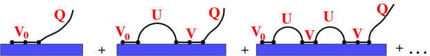
Figure 1: Schematic representation of the series expansion given by Eq. (1)

The GC-partition function of the loops is defined by

$$U(z)=\sum_{m=1}^{\infty}\>\Omega_{m}\>z^{m}=\sum_{m=1}^{\infty}\>\frac{(\mu_{3}z)^{m}}{m^{1-\gamma_{11}}}$$ (2)

where $\Omega_{m}$ is the number of surface $m$-loops (i.e., self-avoiding walks of length $m$ which start and terminate on the surface) configurations. For an isolated $m$-loop this number of configurations is given by $\Omega_{m}=\mu_{3}^{m}m^{\gamma_{11}-1}$ where $\mu_{3}$ is the $3d$ connective constant (in three dimensions, $d=3$, one has $\mu_{3}=4.68$, and the exponent $\gamma_{11}=-0.390$ )Vanderzande . Below we will demonstrate that the exponent $\gamma_{11}$ changes due to the excluded volume interactions between different loops.

The train GC-partition function reads

$$V(z)=\sum_{m=1}^{\infty}\>\Psi_{m}\>z^{m}=\sum_{m=1}^{\infty}\>\frac{(\mu_{2}wz)^{m}}{m^{1-\gamma_{d=2}}}$$ (3)

where the number of train configurations of length $m$ (which are located in the $d=2$ surface plane) is given by $\Psi_{m}=w^{m}\>\mu_{2}^{m}\;m^{\gamma_{d=2}-1}$. Here $\mu_{2}=2.6$ and $\gamma_{d=2}=1.343$ Vanderzande . In Eq. (3) we have taken into account that each adsorbed segment of the chain gains an additional statistical weight $w=\exp(\varepsilon/k_{B}T)\equiv\exp(\epsilon)$, where $T$ is the temperature and the Boltzmann constant $k_{B}$ is set to unity. In what follows the notation $\epsilon$ stands for the dimensionless adsorption energy of a single monomer. In fact, $\epsilon$ denotes the potential well depth of the short-ranged surface potential, defined in the description of our simulation model in Section IV.

The GC-partition function for the chain tail is given by

$$Q(z)=1+\sum_{m=1}^{\infty}\>\Lambda_{m}\>z^{m}=1+\sum_{m=1}^{\infty}\>\frac{(\mu_{3}z)^{m}}{m^{1-\gamma_{1}}}$$ (4)

where the $m$-tail number of configuration equals $\Lambda_{m}=\mu_{3}^{m}\>m^{\gamma_{1}-1}$, and in $d=3$ the exponent $\gamma_{1}=0.680$ Vanderzande .

With the knowledge of the GC partition function, given by Eq.(1), it is possible to calculate the number of weighted configurations of a polymer chain, containing $N$ segments (i.e., its canonical partition function), $\Xi_{N}$. From the generating function method (see, e.g., Sec. $2.4$ in the book by Rudnick and Gaspari Rudnick ) it is well known that at $N\rightarrow\infty$ the coefficient at $z^{N}$ is defined by a singular point (a pole or a branching point) of $\Xi(z)$ which lies closest to the origin. In our case this is a simple pole, $z^{*}$, which is determined from the condition

$$V(z^{*})\>U(z^{*})=1$$ (5)

The principal contribution to this coefficient at $z^{N}$ is $(z^{*})^{-(N+1)}$, i.e., $\Xi_{N}\approx(z^{*})^{-N}$, and so the corresponding free energy

$$F=-T\ln\Xi_{N}=TN\ln z^{*}$$ (6)

In Section II, devoted to the adsorption of a pulled polymer chain, we shall see that an important singularity arises also from the tail generating function. The average fraction of adsorbed monomers, $n=N_{s}/N$ (where $N_{s}$ is the number of adsorbed monomers) which we use as an order parameter for the degree of adsorption, can be calculated then as follows

$$n\equiv\frac{N_{s}}{N}=\frac{1}{N}\;\frac{\partial\>\>\ln\Xi_{N}}{\partial\ln w}=-\frac{\partial\ln z^{*}}{\partial\ln w}$$ (7)

The generating functions, given by Eqs. (2), (3), and (4), can be conveniently expressed in terms of the polylog function Erdelyi . In the Appendix we sketch the properties of the polylog function and its behavior in the vicinity of the singular point. In terms of the polylog function (see Appendix) the basic Eq.(5) is then given by

$$\Phi(\alpha,\mu_{3}z^{*})=\Phi^{-1}(\lambda,\mu_{2}wz^{*})$$ (8)

where the exponents $\alpha=1-\gamma_{11}\approx 1.39>1$ and $\lambda=1-\gamma_{d=2}\approx-0.343<1$. One should note that the exponent $\alpha=1-\gamma_{11}$ corresponds to a loop treated as an isolated one. This is an important feature of the method which handles the main building blocks (loops, trains and tails) as independent objects (see, e.g., Eq.(1)). Nevertheless, in Sec. II.2, following Kafri et al. Kafri , we shall show that by taking into account the excluded volume interaction between a loop and the rest of the chain one ends up with a renormalized value of the exponent $\alpha$ (it increases). This is important because the value of $\alpha$ determines itself the value of the well known surface (or, crossover) exponent $\phi$ in all the basic scaling laws pertaining to polymer adsorption (see below).

Close to the critical point, $z_{c}=z^{*}$ which is defined by $\mu_{3}z_{c}=1$, the l.h.s. of Eq.(8) can be expanded (cf. Eq.(92)) as follows

$$\zeta(\alpha)-a_{\alpha}(1-\mu_{3}z^{*})^{\alpha-1}-b_{\alpha}(1-\mu_{3}z^{*})=\Phi^{-1}(1-\gamma_{d=2},\mu_{2}wz^{*})$$ (9)

with $\zeta(x)$ denoting the Riemann zeta-function. At the critical adsorption point (CAP), $\epsilon_{c}$ and $w_{c}=\exp(\epsilon_{c})$, the solution of Eq. (8) is $z^{*}=z_{c}=1/\mu_{3}$ so that $w_{c}$ is given by the expression

$$\zeta(\alpha)=\Phi^{-1}(1-\gamma_{d=2},\mu_{2}w_{c}/\mu_{3}).$$ (10)

The expansion of Eq.(9) around the critical point, $z^{*}=z_{c}$ and $w=w_{c}$, could be effected by the substitution of $w=w_{c}+\delta$ and $z^{*}=z_{c}-\Delta$ in Eq. (9). Here $\delta$ and $\Delta$ are corresponding infinitesimal increments and we took into account that $z^{*}$ decreases with increasing $w$. Substituting this in Eq. (9) gives

$$\zeta(\alpha)-a_{\alpha}(\mu_{3}\Delta)^{\alpha-1}\approx\Phi^{-1}(1-\gamma_{d=2},\mu_{2}w_{c}z_{c})-\Phi^{-2}(1-\gamma_{d=2},\mu_{2}w_{c}z_{c})\>\>\left[\frac{d}{dx}\;\Phi(1-\gamma_{d=2},x)\right]_{x=\mu_{2}w_{c}z_{c}}\>\delta$$ (11)

Taking into account the condition for the critical point, Eq. (10), as well as the identity Eq. (83), the solution for $z^{*}$ can be recast in the form

$$z^{*}(w)\approx\frac{1}{\mu_{3}}\left[1-\left(\frac{A}{a_{\alpha}}\right)^{1/(\alpha-1)}\>(w-w_{c})^{1/(\alpha-1)}\right]$$ (12)

where the constants

$$A = \frac{\mu_{2}\Phi(-\gamma_{d=2},\mu_{2}w_{c}/\mu_{3})}{\Phi^{2}(1-\gamma_{d=2},\mu_{2}w_{c}/\mu_{3})}$$

$$a_{\alpha} = \frac{\pi}{\Gamma(\alpha)|\sin(\pi\alpha)|},$$ (13)

and $w_{c}$ is defined by Eq. (10). The full numerical solution for the order parameter as well as for the pole $z^{*}(w)$ is displayed in Fig. 2.

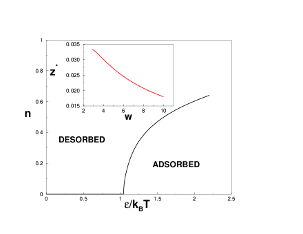
Figure 2: The ’order parameter’ (i.e., the fraction of adsorbed chain segments), $n$, against the surface potential, $\epsilon$, in the absence of detachment force, $f=0$. The inset shows the variation of the fugacity $z^{*}$ with $w=\exp(\epsilon)$, Eq. (8).

Having the solution Eq.(12) at hand, one can use the expression Eq.(7) for the average fraction of adsorbed monomers. After some straightforward calculations one arrives at

$$n(\epsilon)\propto(\epsilon-\epsilon_{c})^{\frac{1}{\alpha-1}-1}$$ (14)

where one has used $w-w_{c}\approx\exp(\epsilon_{c})\>(\epsilon-\epsilon_{c})$. On the other hand, it is well known Vanderzande that the scaling behavior in the vicinity of the critical adsorption energy is described by the crossover exponent $\phi$. Namely, the corresponding scaling relationship is given by

$$n(\epsilon)\propto\begin{cases}N^{\phi-1},\quad&\mbox{at}\quad\epsilon=\epsilon_{c}\\ (\epsilon-\epsilon_{c})^{\frac{1}{\phi}-1}\quad&\mbox{at}\quad\epsilon>\epsilon_{c}\end{cases}$$ (15)

If the result, given by Eq.(14), is compared to that of Eq. (15), it becomes apparent that

$$\phi=\alpha-1$$ (16)

This result, derived first by BirshteinBir , is of principal importance. Here it is derived in the context of self-avoiding chains. As stated above, if the loops are treated as independent non-interacting objects, the exponent $\alpha=1-\gamma_{11}$, so that

$$\phi=-\gamma_{11}\approx 0.39$$ (17)

In Sec. II.2 we shall demonstrate that by taking into account the excluded volume interactions between a loop and the rest of the chain one finds an increase of the values of $\alpha$, and $\phi$, respectively.

II.1 Loops and tails distributions close to criticality

Here we examine how the size distribution of polymer loops and tails looks like close to the critical point of adsorption. The GC-partition function for loops, given by Eq.(2), yields immediately

$$P_{\rm loop}(l)\approx\left.\frac{(\mu_{3}z)^{l}}{l^{\alpha}}\right|_{z=z^{*}}=\frac{(\mu_{3}z^{*})^{l}}{l^{1+\phi}}$$ (18)

where we have used the essential relation between the loop exponent $\alpha$ and the crossover exponent $\phi$, Eq.(16). Close to the critical point, $\mu_{3}z^{*}\leq 1$ (see Eq.(12)) and the $l$-dependence is mainly described by inverse power-law

$$P_{\rm loop}(l)\approx\frac{1}{l^{1+\phi}}$$ (19)

The power-law decay for the loop distribution close to the criticality has been discussed in the early 80s by P.-G.de Gennes PGG . Deeper in the region of adsorption, however, the exponential part in Eq. (18) dominates. Taking into account Eq.(12), one obtains

$$P_{\rm loop}(l)\approx\frac{1}{l^{1+\phi}}\exp\left[-c_{1}(\epsilon-\epsilon_{c})^{1/\phi}\>l\right],$$ (20)

i.e., with increasing adsorption energy $\epsilon$ the size distribution becomes narrower.

It is of interest to note that the size distribution of loops can be reformulated in terms of the distribution $F(h)$ of projected lengths $h$ of the loops between two consecutive monomers residing on the adsorbing surface which was analyzed by Bouchaud and Daoud Bouchaud . The relation between $P_{\rm loop}(l)$ and $F(h)$ is straightforward, namely $F(h)dh=P_{\rm loop}(l)|dl/dh|dh$, where due to the isotropy of loops $h\sim l^{\nu}$ too. Taking these relations into account as well as Eq.(19) one obtains

$$F(h)\approx\frac{1}{h^{1+\phi/\nu}}$$ (21)

This corresponds exactly to the result of Bouchaud and Daoud Bouchaud where such broad distribution was associated with the so-called node-avoiding Levy flight.

The distribution of tails (at the CAP, i.e., at $\mu_{3}z^{*}\leq 1$) is even broader, namely

$$P_{\rm tail}(l)\approx\frac{(\mu_{3}z^{*})^{l}}{l^{\beta}}$$ (22)

where for an isolated tail $\beta=1-\gamma_{1}\approx 0.32$. We will show below (see Eq.(46)) that if the interaction of a tail with the rest of the chain is taken into account this leads to a larger value of $\beta=0.51$. One should be aware, however, that this result, Eq. (22), is only valid for $\epsilon\geq\epsilon_{c}$ since a solution for Eq. (8) does not exist for subcritical values of the adsorption potential. It is clear, however, that even in the subcritical region, $\epsilon<\epsilon_{c}$, there are still monomers which occasionally touch the substrate, creating thus single loops at the expense of the tail length. This affects and modifies therefore the distribution $P_{\rm tail}$ in the vicinity of $\epsilon_{c}$. One can take into account this additional contribution by considering a single loop - tail configuration. Pictorially the latter can be inferred from Fig. 4b where instead of two loops and a tail one should imagine a single loop adjacent to the tail. The partition function of such configuration is given by $Z_{l-t}=\frac{\mu_{3}^{N-l}}{(N-l)^{1+\phi}}\;\frac{\mu_{3}^{l}}{l^{\beta}}$. On the other side, the partition function of a tail conformation with no loops whatsoever (i.e., of a tethered chain) is $Z_{t}=\mu_{3}^{N}\;N^{\gamma_{1}-1}$. Thus the probability $P^{<}_{\rm tail}(l)$ to find a tail of length $l$ next to a single loop of length $N-l$ can be estimated as

$$P^{<}_{\rm tail}(l)=\frac{Z_{l-t}}{Z_{t}}\propto\frac{N^{1-\gamma_{1}}}{l^{\beta}(N-l)^{1+\phi}}.$$ (23)

Evidently, Eq. (23) predicts a singularity (that is, a steep maximum) in the distribution of tails when $l\cong N$. One may expect that in the vicinity of the critical point, $\epsilon\approx\epsilon_{c}$, the observed distribution of tails will be given by an interpolation between the expressions shown in Eq. (22) and Eq. (23). Hence, the overall tail distribution can be represented as

$$P_{\rm tail}(l)=\begin{cases}\frac{1}{l^{\beta}}\exp\left[-c_{1}(\epsilon-\epsilon_{c})^{1/\phi}\;l\right],\quad&\quad\epsilon>\epsilon_{c}\\ \\ \frac{A_{1}}{l^{\beta}}+\frac{A_{2}N^{1-\gamma_{1}}}{l^{\beta}(N-l)^{1+\phi}},\quad&\quad\epsilon=\epsilon_{c}\\ \\ \frac{N^{1-\gamma_{1}}}{l^{\beta}(N-l)^{1+\phi}}.\quad&\quad\epsilon<\epsilon_{c}\end{cases}$$ (24)

Evidently, close to the CAP this distribution is expected to attain a $U$-shaped form with maxima at $l\approx 1$ and $l\cong N$. This shape of $P_{\rm tail}(l)$ has been predicted earlier for a Gaussian chain by Gorbunov et al.Gorbunov . In close analogy with Eq. (24), the distribution of loops reads

$$P_{\rm loop}(l)=\begin{cases}\frac{1}{l^{1+\phi}}\exp\left[-c_{1}(\epsilon-\epsilon_{c})^{1/\phi}\;l\right],\quad&\quad\epsilon>\epsilon_{c}\\ \\ \frac{B_{1}}{l^{1+\phi}}+\frac{B_{2}N^{1-\gamma_{1}}}{l^{1+\phi}(N-l)^{\beta}},\quad&\quad\epsilon=\epsilon_{c}\\ \\ \frac{N^{1-\gamma_{1}}}{l^{1+\phi}(N-l)^{\beta}}.\quad&\quad\epsilon<\epsilon_{c}\end{cases}$$ (25)

In Eqs. (24)-(25) $A_{1},A_{2},B_{1},B_{2}$ are some constants. As we shall see in Section V, the simulation results for $P_{\rm tail}(l),P_{\rm loop}(l)$ are in good agreement with the predictions, Eqs. (24)-(25).

II.1.1 Divergence of the average loop and tail lengths at criticality

The average loop length is defined by the loop GC-partition function, Eq.(2), as

$$L=\left.z\>\frac{\partial\ln U(z)}{\partial z}\right|_{z=z^{*}}=\frac{\Phi(\alpha-1,\mu_{3}z^{*})}{\Phi(\alpha,\mu_{3}z^{*})}$$ (26)

where we have used Eq.(83). Taking into account the polylog function behavior given by Eq.(92) with the requirement that $1<\alpha<2$ as well as the solution for $z^{*}$, Eq.(12), one gets

$$L\approx\frac{\Gamma(2-\alpha)}{\zeta(\alpha)}\>\left(\frac{a_{\alpha}}{A}\right)^{\frac{2-\alpha}{\alpha-1}}\>\frac{1}{(w-w_{c})^{\frac{2-\alpha}{\alpha-1}}}\propto\frac{1}{(\epsilon-\epsilon_{c})^{\frac{1}{\phi}-1}}$$ (27)

where the result Eq.(16) has been used. This result is compatible with the scaling prediction based on Eq. (15). Indeed, close to criticality, $L\approx N/N_{s}$. From Eq.(15) one obtains then the same result, $L\propto(\epsilon-\epsilon_{c})^{1-1/\phi}$. The free energy goes as $F=TN\ln z^{*}\propto-N(\epsilon-\epsilon_{c})^{1/\phi}$ where one has used Eq.(12). On the other hand, the free energy is proportional to the number of adsorption blobs, i.e., $F\propto N/g$, where $g$ is the length (number of segments) of the blob. The adsorption blobs are defined to contain as many monomers $g$ as necessary to be on the verge of adsorption and therefore carry an adsorption energy of the order of $k_{B}T$ each. In result the blob length scales as $g\propto(\epsilon-\epsilon_{c})^{-1/\phi}$. The size of the adsorbed chain perpendicular to the surface, $R_{\perp}$, is nothing but the blob size, that is, $R_{\perp}\approx g^{\nu}$. Thus one obtains

$$R_{\perp}\propto\frac{1}{(\epsilon-\epsilon_{c})^{\nu/\phi}}.$$ (28)

Consider now the average tail length $S$. In terms of the GC-partition function for tails, Eq. (4), it reads

$$S=\left.z\>\frac{\partial\ln Q(z)}{\partial z}\right|_{z=z^{*}}=\frac{\Phi(\beta-1,\mu_{3}z^{*})}{1+\Phi(\beta,\mu_{3}z^{*})}$$ (29)

with the exponent $\beta=1-\gamma_{1}=0.32<1$. This value of the exponent $\beta$ does not allow for the interaction of the tail with other building blocks of the adsorbed chain and will be corrected in Sec.II.2. Using the results, Eqs. (92) and (12), the expression for the average tail length Eq.(29) can be recast in the form

$$S\approx(1-\beta)\left(\frac{a_{\alpha}}{A}\right)^{\frac{1}{\alpha-1}}\>\frac{1}{(w-w_{c})^{\frac{1}{\alpha-1}}}\propto\frac{1}{(\epsilon-\epsilon_{c})^{\frac{1}{\phi}}}$$ (30)

Notably, the exponent $\beta$ drops out of this expression. The corresponding tail size $R_{\rm S}\sim S^{\nu}$ scales as

$$R_{\rm S}\propto\frac{1}{(\epsilon-\epsilon_{c})^{\nu/\phi}}$$ (31)

Note that the tail size, Eq.(31), scales exactly like the blob (and not the loop!) size, Eq. (28).

II.2 Role of interacting loops and tails

As mentioned above, the exponent $\alpha$, which governs the numbers of loops in the configuration of adsorbed polymer, determines also the crossover exponent $\phi$ so that it is of prime importance to know the exact value of $\alpha$. If the surface loops are treated as isolated objects (i.e., loop-loop or loop-tail interactions are ignored), the exponent $\alpha=1-\gamma_{11}=1.39$. Recently Kafri et al. Kafri have shown in the context of DNA melting that the interaction of a loop with the rest of the chain increases the loop exponent $\alpha$. In their work the authors of ref. Kafri essentially used some results of the renormalization theory of arbitrary polymer graphs, developed earlier by Duplantier Duplantier . This approach makes it possible to treat also polymer chains which are grafted onto a solid surface. Here we give a short sketch of Duplantier’s results for a polymer graph located close to the surface and then demonstrate how the loop-loop and loop-tail interactions lead to the enhancement of the effective surface loop exponent.

For an arbitrary self-avoiding polymer graph ${\cal G}$, which is grafted on the surface, it has been shown Duplantier that the total number of configurations is given by the standard asymptotic expression:

$$Z({\cal G})=\mu_{3}^{N}\>N^{\gamma^{s}-1}$$ (32)

where $N=\sum_{j=1}^{\cal N}M_{j}$ is the total length of the graph made of ${\cal N}$ chains (or edges) of length $M_{j}$. The surface exponent $\gamma^{s}$ is given by the following general relationship

$$\gamma^{s}=1-\nu(d{\cal L}+{\cal L}_{s}+{\cal V}_{s}-1)+\sum\limits_{k\geq 1}\>(n_{L}\sigma_{k}+n_{k}^{s}\sigma_{L}^{s})$$ (33)

where $\nu$ is the Flory exponent and $d$ stands for the space dimensionality. In Eq. (33) ${\cal L}$ is the total number of independent constitutive polymer loops in the graph ${\cal G}$ (i.e., the surface loops are not included in ${\cal L}$). ${\cal L}_{s}$ is the total number of extremities of polymer lines upon contact to the surface. $n_{k}$ and $n_{k}^{s}$ are the numbers of bulk and surface vertices of order $k$ respectively, thus ${\cal L}_{s}=\sum_{k\geq 1}k\>n_{k}^{s}$. ${\cal V}_{s}$ gives the number of surface vertices, i.e., ${\cal V}_{s}=\sum_{k\geq 1}n_{k}^{s}$. Finally, $\sigma_{k}$ and $\sigma_{k}^{s}$ are critical bulk and surface exponents which correspond to the $k$-arm vertices. In $d<4$ these exponents can be calculated analytically via the $\varepsilon$-expansion but some of them could be also expressed in terms of the conventional exponents $\nu$, $\gamma$, $\gamma_{1}$ and $\gamma_{11}$ Duplantier . Figure 3 gives an example of a polymer graph with the specification of its topological elements.

The number of configurations given by Eq.(32) holds when the lengths of all components $M_{a}$ are large and comparable to the total length $N$. As long as at least one of them becomes small, i.e. $M_{a}\ll N$, then one gets

$$Z({\cal G})=\mu_{3}^{N}\>N^{\gamma^{s}-1}\>G\left(\frac{M_{1}}{N},\frac{M_{2}}{N},\dots,\frac{M_{\cal N}}{N}\right)$$ (34)

where the scaling function $G(x_{1},x_{2},\dots,x_{\cal N})$ has a singularity, provided any of the arguments $x_{a}$ goes to zero. In fact, in this limit the polymer graph changes its topology and, therefore, the surface exponent $\gamma^{s}$ changes too. In the next subsection we show how these results could be used to calculate the effective exponent $\alpha$ which takes into account the interaction of a surface loop with the rest of the chain.

Figure 3: A polymer graph located close to the surface has the following topological characteristics: ${\cal L}=1$, ${\cal L}_{s}=9$, ${\cal V}_{s}=4$, $n_{1}=3$, $n_{3}=2$, $n_{1}^{s}=1$, $n_{2}^{s}=1$, $n_{3}^{s}=2$. One surface vertex is fixed whereas the other vertices may move freely.

II.2.1 Surface loop embedded in an adsorbed chain

Consider the configurations of a chain (tethered with one end on the surface) in the vicinity of the adsorption critical point (see Fig. 4). Let $M$ be the length of a surface loop while $K$ measures the length of the rest of the chain, i.e., $M+K=N$. The number of configurations of the polymer graph, depicted in Fig.4a, is

$$Z=\mu_{3}^{M+K}\>(M+K)^{\gamma_{a}^{s}-1}\>G\left(\frac{M}{M+K}\right)$$ (35)

where $\gamma_{a}^{s}$ is the exponent which could be calculated using Eq.( 33) (see below) and the scaling function $G(x)\approx 1$ for large $M$ and $K$. In the case when $M/K\rightarrow 0$ one has a crossover to the polymer graph shown in Fig 4b where the number of configurations $Z\sim\mu_{3}^{K}\>(K)^{\gamma_{a}^{s}-1}\>(1/K)^{\gamma_{a}^{s}-\gamma_{b}^{s}}$ (with $\gamma_{b}^{s}$ being the surface exponent of the corresponding graph). These arguments fix the form of the scaling function which can be written as

$$G(x)\approx\begin{cases}x^{\gamma_{a}^{s}-\gamma_{b}^{s}},\quad&\mbox{at}\quad x\ll 1\\ 1,\quad&\mbox{at}\quad x\approx 1\end{cases}$$ (36)

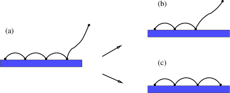
Figure 4: An array of surface loops close to criticality. One of the surface loops of length $M$ in the limit $M/N\ll 1$ is contracted, changing the topology of the polymer graph from (a) to (b). This contraction procedure makes it possible to derive the scaling function $G(x)$. By similar contraction of a tail the graph goes over from (a) to (c).

In the case of a small surface loop, embedded in an adsorbed polymer, with $M\gg 1$ and $K\gg 1$ (but with $M/K\ll 1$) one obtains for the total number of configurations

$$Z\sim\mu_{3}^{M+K}\>K^{\gamma_{a}^{s}-1}\left(\frac{M}{K}\right)^{\gamma_{a}^{s}-\gamma_{b}^{s}}\sim\mu_{3}^{M}\>M^{\gamma_{a}^{s}-\gamma_{b}^{s}}\>\>\mu_{3}^{K}\>K^{\gamma_{b}^{s}-1}.$$ (37)

The last result indicates that the total partition function may be factorized to $Z\sim Z_{\rm loop}\>Z_{\rm rest}$ where $Z_{\rm loop}$ and $Z_{\rm rest}$ are the partition functions of the small loop and the rest of the chain, respectively. Thus, using the notations of Eq.(2), one obtains $\Omega_{n}=\mu_{3}^{n}/n^{\gamma_{b}^{s}-\gamma_{a}^{s}}$, i.e., the effective exponent $\alpha$ becomes

$$\alpha=\gamma_{b}^{s}-\gamma_{a}^{s}.$$ (38)

Now we are in a position to determine the exponents $\gamma_{a}^{s}$ and $\gamma_{b}^{s}$. Let us assume that the polymer graph in Fig. 4a is made of ${\cal N}$ subchains (${\cal N}-1$ being loops and $1$ - a tail). The topological characteristics can be specified as follows: ${\cal L}=0$, ${\cal L}_{s}=2{\cal N}-1$, ${\cal V}_{s}={\cal N}$, $n_{1}=1$, $n_{1}^{s}=1$, $n_{2}^{s}={\cal N}-1$. Earlier it has been shown Duplantier that the critical exponent $\sigma_{2}^{s}=2\nu-1$. With these values Eq.(33) yields

$$\gamma_{a}^{s}=2-{\cal N}(\nu+1)+\sigma_{1}+\sigma_{1}^{s}$$ (39)

The corresponding expression for $\gamma_{b}^{s}$ can be obtained from Eq. (39) by the substitution ${\cal N}\rightarrow{\cal N}-1$. This yields

$$\gamma_{b}^{s}=3+\nu-{\cal N}(\nu+1)+\sigma_{1}+\sigma_{1}^{s}$$ (40)

The final expression for the exponent $\alpha$, given by Eq. (38), then reads

$$\alpha=\gamma_{b}^{s}-\gamma_{a}^{s}=\nu+1.$$ (41)

With this theoretical prediction the value of the crossover exponent, given by Eq. (16), is determined as:

$$\phi=\alpha-1=\nu=0.588$$ (42)

where we have taken the best numerical estimate for the Flory exponent $\nu$ at $d=3$ Vanderzande . A comparison of Eq.(42) with Eq. (17) leads to the important conclusion that, depending on the range of the excluded volume interaction, the value of $\phi$ may vary significantly. Indeed, if the interactions affect beads from the same surface loop only then $\phi$ is given by Eq.(17), otherwise (i.e., when the beads from all loops interact) the value of $\phi$ will be enhanced markedly (see Eq. (42)).

One should emphasize, however, that Eq. (41) does not give an exact value for the exponent $\alpha$, but rather an upper limit only. Indeed, the total number of configurations, given by Eq. (37), is estimated by a factorized expression for the partition function which takes into account the contribution of a loop and the rest of the chain. As a matter of fact this is a Mean Field approach which overestimates interactions at the expense of correlations, reducing thus the total number of configurations of a loop. The latter is reflected by an increase of $\alpha$. The precise value of $\alpha$ therefore satisfies the inequality $1-\gamma_{11}<\alpha<1+\nu$. In the special case of a Gauissian chain both the lower and upper limits for $\alpha$ merge while for a phantom chain one has $\gamma_{11}=-0.5$ (cf. Section 6.2 in Duplantier ) and $\nu=0.5$. Thus, for Gaussian chains one obtains the well known value $\phi=0.5$.

Following the same way of reasoning, one may expect that the exponent for the tail, $\beta$ (see Eq. (29)), is also renormalized due to interaction with the rest of the adsorbed chain. Tail contraction when going from (a) to (c) in Fig. 4 enables one to obtain for the renormalized $\beta$-exponent the following relationship

$$\beta=\gamma_{c}^{s}-\gamma_{a}^{s}$$ (43)

where $\gamma_{c}^{s}$ is the surface exponent of the polymer graph given in Fig. 4c. Again, if the polymer graph given in Fig. 4a is made of ${\cal N}$ chains then the exponent $\gamma_{c}^{s}$ for the graph Fig. 4c becomes

$$\gamma_{c}^{s}=3-\nu-{\cal N}(\nu+1)+2\sigma_{1}^{s}$$ (44)

Taking into account Eq. (39), one obtains $\beta=1-\nu+\sigma_{1}^{s}-\sigma_{1}$, whereby the critical exponents (see Duplantier ) are given by

$$\sigma_{1} = \frac{\gamma-1}{2}$$

$$\sigma_{1}^{s} = \nu+\gamma_{1}-\frac{\gamma+1}{2}$$ (45)

The calculation gives finally

$$\beta=\gamma_{1}-\gamma+1$$ (46)

with $\gamma_{1}\approx 0.68$ and $\gamma\approx 1.17$ so that $\beta\approx 0.51$. As expected, the value of the $\beta$-exponent increases as compared to the “isolated tail” case, $\beta=1-\gamma_{1}\approx 0.32$.

II.2.2 Comparison with other results

The result, given by Eq. (42), deserves a more detailed discussion. One should point out that, generally, the value of $\phi$ for the good solvent case in three dimension has been so far fairly controversial. For example, Monte-Carlo (MC) data (albeit for relatively short chains $N\leq 100$) on a diamond lattice yield $\phi=0.588\pm 0.03$ Eisenriegler which is in complete agreement with Eq.(42). A recent MC-investigation Descas has suggested that the uncertainty in the value of $\phi$ might be related to the limited accuracy in the determination of the critical adsorption energy $\epsilon_{c}$. Namely, for the bond fluctuation model (BFM), which has been used by Descas, Sommer and Blumen Descas , $\epsilon_{c}$ ranges between $0.98$ and $1.01$, i.e., within $\pm 2.5\%$. This relatively small change leads to significant variation of $\phi$ between $0.5$ and $0.59$. The same authors have shown that the set of parameters, $\epsilon_{c}=1.01$ and $\phi=0.59$, leads to a more accurate scaling prediction. The adsorption of the tethered SAW chain on a simple cubic lattice for chain lengths of up to $N=1000$ (by means of the so-called “scanning method”) gives: $\phi=0.53\pm 0.007$ Meirovitch . In yet another MC-study, based on the pruned-enriched Rosenbluth method (PERM) Grassberger_1 , it was found that $\phi$ is pretty close to $0.5$. However, in a more recent study of the same author Grassberger_2 one determined for $\phi$ an even smaller value: $\phi=0.484\pm 0.002$. The value $\phi=0.5$ was also been supported by the MC-simulation results based on the off-lattice model Metzger .

The analytical methods for calculation of $\phi$ are based on the field-theoretical renormalization group (RG) study of the semi-infinite $n$-vector model in the $n\rightarrow 0$ limit. In earlier investigations Diehl_1 ; Diehl_2 ; Eisen the $\varepsilon$-expansion (where $\varepsilon=4-d$) up to order $\varepsilon^{2}$ lead to the prediction $\phi=0.67$ which deviates widely from all MC-findings. In a more recent investigation the so-called massive field-theory approach at fixed $d$ (i.e., the $\varepsilon$-expansion has been avoided) was extended to systems with surfaces Shpot_1 ; Shpot_2 . The result for the crossover exponent reads $\phi\approx 0.52$. Thus we believe that the present study elucidates the origin for the diversity of results concerning the precise value of $\phi$ and provides a physical background of it.

III Adsorption under external detaching force

The adsorption of a Gaussian chain on a solid plane under detaching force acting on the chain end has been studied first by Skvortsov, Gorbunov and Klushin Skvortsov_1 ; Skvortsov_2 in the early 90s. For a Gaussian chain the problem can be solved rigorously even for a finite chain length $N$. The adsorption-desorption transition is of the first order, however, phase coexistence and metastable states are absent.

Below we apply the GC - ensemble approach to the case of self-avoiding polymer chain adsorption under the presence of detaching force. Again, the problem has much in common with the unzipping transition of double-stranded DNA Kafri . When a force $f$ is applied to the free end of the tethered chain, the tail GC partition function in Eq.(1) changes. The total GC-partition function is then given by

$$\Xi(z)=\frac{V_{0}(z)\>R(z)}{1-V(z)U(z)}$$ (47)

where the tail GC - partition function now takes on the form

$$R(z)=1+\sum_{m=1}^{\infty}\>\Xi_{\rm tail}(m)\>z^{m}$$ (48)

In Eq.(48) $\Xi_{\rm tail}(m)$ is the canonical partition function of the tail under applied force:

$$\Xi_{\rm tail}(m)=\frac{\mu_{3}^{m}}{m^{\beta}}\>\int d^{3}r\>P_{m}({\bf r})\>\exp\left(fr_{\perp}/T\right).$$ (49)

Here we take into account that the pulling force is directed perpendicular to the plane (in $r_{\perp}$-direction). In Eq. (49) $P_{m}({\bf r})$ is the end-to-end distance probability distribution function (PDF). To estimate this function on large distances from the solid plane, i.e., at $r_{\perp}\gg R_{m}\approx am^{\nu}$ (here and in what follows $a$ denotes the length of a Kuhn-segment), we assume, following Kreer et al. Binder , that under this condition the PDF is given by the des Cloizeaux expression DesCloizeaux for the bulk:

$$P_{m}({\bf r})=\frac{1}{R_{m}^{3}}\>F\left(\frac{{\bf r}}{R_{m}}\right)$$ (50)

where the scaling function $F(x)$ is

$$F(x)=Bx^{t}\>\exp\left(-Dx^{\delta}\right).$$ (51)

In Eq. (51) $B$ and $D$ are constants while the exponents $\delta$ and $t$ are given by

$$\delta=\frac{1}{1-\nu}$$ (52)

and

$$t=\frac{\beta-d/2+d\nu}{1-\nu}.$$ (53)

Here $\beta=1-\gamma_{1}$ is the tail surface exponent and $d=3$. Note that in the limit $r_{\perp}\gg R_{m}$ the only difference between the PDFs in the bulk and in the semi-infinite case lies in the fact that instead of the exponent $\gamma$ in Eq. (53) one has $\gamma_{1}$. The integration over the coordinates parallel to the plane in Eq.(49) is readily carried out and one obtains

$$\Xi_{\rm tail}(m) = \frac{\mu_{3}^{m}}{m^{\beta}}\>\frac{C}{R_{m}}\int\limits_{0}^{\infty}dr_{\perp}\>\left(\frac{r_{\perp}}{R_{m}}\right)^{2+t-\delta}\>\exp\left[-D\left(\frac{r_{\perp}}{R_{m}}\right)^{\delta}+\frac{fr_{\perp}}{T}\right]$$ (54)

$$= C\>\frac{\mu_{3}^{m}}{m^{\beta}}\>\int\limits_{0}^{\infty}dx\>x^{2+t-\delta}\exp\left(-Dx^{\delta}+{\tilde{f}}_{m}x\right)$$

where the normalization constant $C=\delta D^{(3+t)/\delta-1}/\Gamma[(3+t)/\delta-1]$. The integral in Eq. (54) can be tackled by the saddle point method (since ${\tilde{f}}_{m}\equiv fR_{m}/T\gg 1$). The saddle point itself is defined by the value $x_{\rm sp}=({\tilde{f}}_{m}/(\delta D))^{1/(\delta-1)}\sim{\tilde{f}}_{m}^{1/\nu-1}$, or, in terms of the $r_{\perp}$-variable,

$$r_{\perp}^{\rm sp}\approx R_{m}\>\left({\tilde{f}}_{m}\right)^{1/\nu-1}\approx am\left(\frac{fa}{T}\right)^{1/\nu-1}$$ (55)

which is nothing but the well-known Pincus deformation law Gennes . Finally, Eq. (54) becomes

$$\Xi_{\rm tail}(m)=a_{1}\>({\tilde{f}})^{\theta}\>\frac{\mu_{3}^{m}}{m^{\beta-\theta\nu}}\>\exp\left(a_{2}{\tilde{f}}^{1/\nu}m\right)$$ (56)

with $a_{1}$ and $a_{2}$ being constants, the dimensionless force ${\tilde{f}}\equiv fa/T$, and the exponent $\theta=(2+t-3\delta/2)/(\delta-1)$. Thus the GC-partition function , Eq. (48), can be written as

$$R(z) = 1+a_{1}\>{\tilde{f}}^{\theta}\>\sum_{m=1}^{\infty}\>\frac{1}{m^{\psi}}\>\left[z\mu_{3}\exp(a_{2}{\tilde{f}}^{1/\nu})\right]^{m}$$ (57)

$$= 1+a_{1}\>{\tilde{f}}^{\theta}\>\Phi(\psi,z\mu_{3}\exp(a_{2}{\tilde{f}}^{1/\nu}))$$

where we have defined the new exponent

$$\psi=\beta-\nu\theta=\frac{d-1}{2}-(d-2)\nu.$$ (58)

One should point out that the exponent $\beta$ drops out from the final expression for $\psi$ which for $d=3$ is defined as $\psi=1-\nu$.

It is evident from Eq. (57) that (cf. Eq.(92)) at $z\rightarrow\mu_{3}^{-1}\>\exp(-a_{2}{\tilde{f}}^{1/\nu})$ the tail GC-partition function has a branch point at $z=z^{\#}$, i.e.

$$R(z)\sim a_{1}\>({\tilde{f}})^{\theta}\>\frac{\Gamma(1-\psi)(z^{\#})^{1-\psi}}{\left[z^{\#}-z\right]^{1-\psi}}$$ (59)

where $1-\psi<1$ and

$$z^{\#}=\mu_{3}^{-1}\>\exp(-a_{2}{\tilde{f}}^{1/\nu}).$$ (60)

Turning back to the total GC-partition function, Eq.(47), one may conclude that $\Xi(z)$ has two singularities on the real axis ${\rm Re}z$: the pole $z^{*}$ which is defined by Eq.(5), and the branch point $z^{\#}$ given by Eq. (60). It is well known (see, e.g., Sec. 2.4.3 in Rudnick ) that in the thermodynamic limit, $N\rightarrow\infty$, the contribution to the coefficient of $z^{N}$ (i.e., to $\Xi_{N}$) consists of contributions by the pole and by the branch singular points, i.e.

$$\Xi_{N}\sim C_{1}\>(z^{*})^{-(N+1)}+\frac{C_{2}}{\Gamma(1-\psi)}\>N^{-\psi}\>(z^{\#})^{-(N+1-\psi)}$$ (61)

The singular points, $z^{*}$ and $z^{\#}$, are involved in Eq.(61) with large negative exponents. Hence, for large $N$ only the smallest of these points matters. On the other hand, $z^{*}$ depends on the dimensionless adsorption energy $\epsilon$ only (or, on $w=\exp(\epsilon)$) whereas $z^{\#}$ is controlled by the dimensionless external force ${\tilde{f}}$ (cf., Eq.(60)). Therefore, in terms of the two control parameters, $\epsilon$ and ${\tilde{f}}$, the equation

$$z^{*}(\epsilon)=z^{\#}({\tilde{f}})$$ (62)

determines the critical line of transition between the adsorbed phase and the force-induced desorbed phase. In the following this line will be referred to as the detachment line. The controll parameters, $\epsilon_{D}$ and ${\tilde{f}}_{D}$, which satisfy Eq. (62), will be named detachment energy and detachment force, respectively. On the detachment line the system undergoes a first-order phase transition. The detachment line at ${\tilde{f}}_{D}\rightarrow 0$ terminates in the critical adsorption point, $\epsilon_{c}$, where the transition becomes of second order. In the vicinity of the critical adsorption point the detachment force ${\tilde{f}}_{D}$ behaves as

$${\tilde{f}}_{D}\sim(\epsilon-\epsilon_{c})^{\nu/\phi}$$ (63)

where we have used Eq.(62) as well as Eqs. (12) and (60).

III.1 Order parameter

Let us study first how the fraction of adsorbed monomers $n=N_{s}/N$, which we use as an order parameter, depends on the pulling force at fixed value of the contact energy $\epsilon_{1}>\epsilon_{c}$. For ${\tilde{f}}<{\tilde{f}}_{D}$ it is clear that $z^{*}<z^{\#}$ and the first term in Eq. (61) dominates over the second one. In this case the order parameter

$$n=-\left.\frac{\partial\ln z^{*}(w)}{\partial\ln w}\right|_{w=\exp(\epsilon_{1})}$$ (64)

is constant independent of the force. At ${\tilde{f}}>{\tilde{f}}_{D}$ (i.e., after crossing the detachment line) $z^{*}>z^{\#}$ and the second term in Eq. (61) prevails. Since $z^{\#}$ is $w$-independent, it is evident that $n=0$, i.e., the polymer is totally detached. In result, the $n$ vs. ${\tilde{f}}$ dependence resembles a step - function with a jump at ${\tilde{f}}={\tilde{f}}_{D}$.

Now let us fix the force ${\tilde{f}}={\tilde{f}}_{1}$ and investigate how the order parameter $n$ depends on the adsorption energy $\epsilon$ or on the fugacity $w$. Again, Eq.(62) at ${\tilde{f}}={\tilde{f}}_{1}$ defines a detachment energy $\epsilon_{D}$. At $\epsilon<\epsilon_{D}$ one has still $z^{\#}<z^{*}$ and the second term in Eq. (61) dominates so that the chain is completely desorbed (i.e., $n=0$). At $\epsilon>\epsilon_{D}$ only the first term in Eq.(61) survives so that the relationship $n$ vs. $\epsilon$ follows the conventional adsorption dependence without any force-influence. The transition at $\epsilon=\epsilon_{D}$ is of first order whereby the order parameter jump grows as the force ${\tilde{f}}_{1}$ increases.

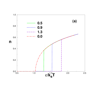
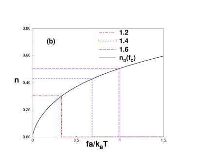
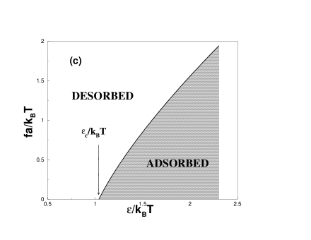
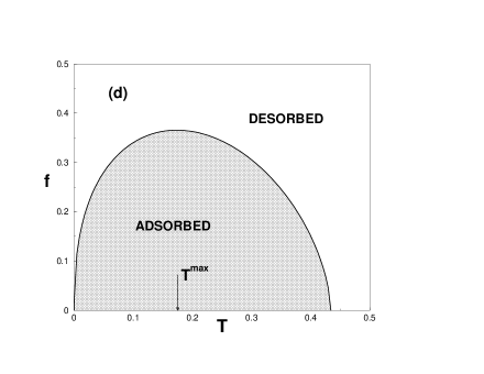
Figure 5: The ’order parameter’ , $n$, against the: (a) energy of adsorption $\epsilon$ ($f$ is given as a parameter); (b) - against the pulling force $f$, with $\epsilon$ a parameter. Vertical lines denote the discontinuous jumps of $n$, indicating a $1^{st}-$ order transition. The $n_{D}(f_{D})$ (full line) in (b) denotes the order parameter value at the detachment line. (c) The phase diagram of the adsorption-desorption transition under puling force $f$ in dimensionless units. An arrow at $\epsilon_{c}$ denotes the point of critical adsorption for $f=0$. (d) The reentrant phase diagram - the same as in (c) but with force against temperature in dimensional units at fixed value of $\epsilon>\epsilon_{c}$. The largest force $f$ for which chain adsorption may still take place occurs at temperature $T^{max}$, as indicated by an arrow.

In Figure 5a,b we show the predicted variation of the order parameter for an infinitely long chain, following from the present consideration. The boundary of the region of adsorbtion, shown in the phase diagram in Figure 5c, denotes the line of critical values of detachment force for any given attraction of the substrate as described by Eq. (62).

The adsorption-desorption first order phase transition under pulling force has a clear dichotomic nature (i.e., it follows an “either - or” scenario): in the thermodynamic limit $N\rightarrow\infty$ there is no phase coexistence! The configurations are divided into adsorbed and detached (or stretched) dichotomic classes. The metastable states are completely absent. Basically, this is in line with the general thermodynamic principles which argue that in thermal equilibrium the thermodynamic potentials are convex functions of their order parameters. This exclude multiple minima and metastable states Binder_Review .

III.2 Reentrant behavior of the phase diagram

The results given in Section III.1 demonstrate that the detachment line on the phase diagram is a monotonous function in terms of the dimensionless quantities ${\tilde{f}}_{D}$ vs. $\epsilon_{D}$. Recently, it has been revealed that the detachment line, when represented in terms of dimensional variables, force $f_{D}$ versus temperature $T$, goes (at the relatively low temperature) through a maximum, that is, the desorption transition shows a reentrant behavior! Below we demonstrate that this result follows directly from our theory.

First, one should note that the low temperature limit implies large values of the ratio $\epsilon=\varepsilon/k_{B}T$. On the other hand, the solution $z^{*}(w)$, which results from Eq.(8), goes to zero, i.e., $z^{*}\rightarrow 0$, when $\varepsilon\rightarrow\infty$. One may assume that under these conditions $z^{*}\mu_{2}{\rm e}^{\epsilon}\rightarrow 1^{-}$ (this will be proven a posteriori). Then the polylog function in the l.h.s. of Eq.(8) reads $\Phi(\alpha,\mu_{3}z^{*})\approx\mu_{3}z^{*}$ but $\Phi^{-1}(\lambda,\mu_{2}wz^{*})\approx c_{1}(1-\mu_{2}wz^{*})^{1-\lambda}$ (where we have used Eq. (92) and the fact that $\lambda<1$). Taking into account Eq.(8), one arrives at the following result

$$\mu_{3}z^{*}\approx c_{1}(1-\mu_{2}wz^{*})^{1-\lambda}$$ (65)

This equation determines the function $z^{*}(w)$ at large $w$. To zero-order approximation the solution reads $z^{*}_{(0)}\approx(\mu_{2}w)^{-1}$. Within the first order approximation $z^{*}_{(1)}\approx(\mu_{2}w)^{-1}-\delta$ where the decrement $\delta$ is found as $\delta=(1/\mu_{2}w)(\mu_{3}/\mu_{2}w)^{1/(1-\lambda)}$. This result is consistent with the assumption $z^{*}\mu_{2}{\rm e}^{\epsilon}\rightarrow 1^{-}$ so that the solution of Eq. (65) in the main approximation can be written as

$$z^{*}\approx\frac{1}{\mu_{2}}\>{\rm e}^{-\epsilon}$$ (66)

By making use of this solution as well as of the result given by Eq.(60) in the Eq.(62), the detachment line at large dimensionless detachment energy $\epsilon_{D}\equiv\varepsilon/T$ and force ${\tilde{f}}_{D}\equiv af_{D}/T$ can be written as

$${\tilde{f}}_{D}=\frac{1}{a_{2}^{\nu}}\>\left[\epsilon_{D}-\ln\left(\frac{\mu_{3}}{\mu_{2}}\right)\right]^{\nu}.$$ (67)

Thus, in terms of the dimensionless controll parameters ${\tilde{f}}_{D}$ increases as the energy $\epsilon_{D}$ increases. Notably, however, if the same detachment line is represented in terms of the dimensional control parameters, detachment force $f_{D}$ vs. detachment temperature $T_{D}$ (with the dimensional adsorption energy $\varepsilon_{0}$ being fixed), one encounters a nonmonotonic behavior

$$f_{D}=\frac{T_{D}}{a}\>\left[\frac{\varepsilon_{0}}{T_{D}}-\ln\left(\frac{\mu_{3}}{\mu_{2}}\right)\right]^{\nu}$$ (68)

which is shown in Fig. 5d. The curve given by Eq.(68) goes through a maximum at a temperature given by

$$T_{D}^{\rm max}=\frac{(1-\nu)\varepsilon_{0}}{\ln\left(\frac{\mu_{3}}{\mu_{2}}\right)}.$$ (69)

Such nonmonotonic behavior is termed reentrant and can be observed in the DNA unzipping process Maritan ; Seno ; Shakhnovich as well as in the case of stretched polymer adsorption on solid surfaces Mishra ; Krawczyk . At very low $T$, however, the expression, Eq. (50), for $P_{m}({\bf r})$ DesCloizeaux predicts divergent chain deformation Seno , i.e., it becomes unphysical. One can readily show that in this case the correct behavior is given by $fa=\varepsilon_{0}+T\ln(\mu_{3}/\mu_{2})$.

III.3 Average loop and tail lengths close to the detachment line

As long as the adsorption energy $\epsilon>\epsilon_{c}$ (or $w>w_{c}$), the average loop length $L$ remains finite upon the detachment line crossing Namely, at ${\tilde{f}}<{\tilde{f}}_{D}$ the fugacity $z=z^{*}(w)$ and the average loop length are given by

$$L=\left.z\>\frac{\partial\ln U(z)}{\partial z}\right|_{z=z^{*}(w)}=\frac{\Phi\left(\alpha-1,\mu_{3}z^{*}(w)\right)}{\Phi\left(\alpha,\mu_{3}z^{*}(w)\right)}.$$ (70)

Thus, at ${\tilde{f}}<{\tilde{f}}_{D}$ the force does not effects the loop length. At ${\tilde{f}}>{\tilde{f}}_{D}$ the fugacity is given by $z=z^{\#}({\tilde{f}})$ where $z^{\#}$ is determined from Eq. (60). In this case the average loop length reads

$$L=\left.z\>\frac{\partial\ln U(z)}{\partial z}\right|_{z=z^{\#}({\tilde{f}})}=\frac{\Phi\left(\alpha-1,\mu_{3}z^{\#}({\tilde{f}})\right)}{\Phi\left(\alpha,\mu_{3}z^{\#}({\tilde{f}})\right)}$$ (71)

Recall, that at $\epsilon>\epsilon_{c}$ and ${\tilde{f}}>{\tilde{f}}_{D}$ we have $\mu_{3}z^{\#}<\mu_{3}z^{*}<1$. In this case the function given by Eq. (71) declines when the force grows - see Figure 6a.

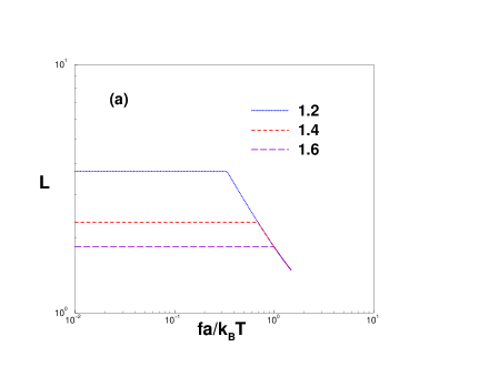
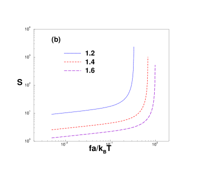
Figure 6: Variation of the average loop size, $L$, with detachment force strength $f$ for several values of the adsorption energy $\epsilon$ (given as a parameter). (b) Mean tail size $S$ against $f$ at different substrate attraction $\epsilon$.

In contrast, the average tail length $S$ diverges in the vicinity of the detachment line. Indeed, at ${\tilde{f}}<{\tilde{f}}_{D}$ the average tail length is given by

$$S=\left.z\>\frac{\partial\ln R(z)}{\partial z}\right|_{z=z^{*}(w)} = \frac{a_{1}{\tilde{f}}^{\theta}\Phi\left(\psi-1,\mu_{3}z^{*}(w)\exp(a_{2}{\tilde{f}}^{1/\mu})\right)}{1+a_{1}{\tilde{f}}^{\theta}\Phi\left(\psi,\mu_{3}z^{*}(w)\exp(a_{2}{\tilde{f}}^{1/\mu})\right)}$$ (72)

$$\approx \frac{1}{\left[1-\mu_{3}z^{*}\exp(a_{2}{\tilde{f}}^{1/\mu})\right]}$$

because $\psi<1$ and $\mu_{3}z^{*}\exp(a_{2}{\tilde{f}}^{1/\mu})\leq 1$ (cf. Eq. (92)). In the vicinity of the detachment line $1-\mu_{3}z^{*}(w)\exp(a_{2}{\tilde{f}}^{1/\mu})\approx({\tilde{f}}_{D}-{\tilde{f}})/(\nu{\tilde{f}}_{D})$ and, therefore,

$$S\propto\frac{{\tilde{f}}_{D}}{{\tilde{f}}_{D}-{\tilde{f}}}.$$ (73)

At ${\tilde{f}}\geq{\tilde{f}}_{D}$ the fugacity $z=z^{\#}({\tilde{f}})$ and hence,

$$S=\left.z\>\frac{\partial\ln R(z)}{\partial z}\right|_{z=z^{\#}({\tilde{f}})}\rightarrow\infty.$$ (74)

The divergence in Eq.(74) follows immediately from Eq.(59) which holds in the thermodynamical limit. In practice, however, for a large but finite chain length $S\rightarrow N$ at ${\tilde{f}}\geq{\tilde{f}}_{D}$. Thus, despite the abrupt first order phase transition, as far as the order parameter $n$ is concerned, the detachment in terms of the tail length $S$ starts diverging already at ${\tilde{f}}\leq{\tilde{f}}_{D}$ as one comes close to the critical detachment force ${\tilde{f}}_{D}$.

III.4 Latent heat variation upon detachment

What is the internal energy change while crossing the detachment line? At ${\tilde{f}}>{\tilde{f}}_{D}$ the stretching energy $E$ follows the Pincus law, so that

$$E({\tilde{f}}={\tilde{f}}_{D}+0)=NT{\tilde{f}}_{D}^{1/\nu}$$ (75)

In the adsorbed phase

$$E({\tilde{f}}={\tilde{f}}_{D}-0)=-NT\>\epsilon_{D}\>n(w_{D})$$ (76)

In result, the latent heat $q$, consumed upon detachment (or, due to force-induced desorption,) reads

$$q\equiv E({\tilde{f}}={\tilde{f}}_{D}+0)-E({\tilde{f}}={\tilde{f}}_{D}-0)=NT\left[{\tilde{f}}_{D}^{1/\nu}+\epsilon_{D}\>n(w_{D})\right]>0$$ (77)

i.e., the heat is absorbed by the system during the force -induced desorption. In the vicinity of the critical point ${\tilde{f}}_{D}\sim(\epsilon-\epsilon_{c})^{\nu/\phi}$ and $n\sim(\epsilon-\epsilon_{c})^{1/\phi-1}$, thus to a leading order

$$q\approx NT\epsilon_{c}\>(\epsilon-\epsilon_{c})^{1/\phi-1}.$$ (78)

IV Monte Carlo Simulation Model

We have investigated the force induced desorption of a polymer by means of extensive Monte Carlo simulations. We use a coarse grained off-lattice bead-spring model MC_Milchev which has proved rather efficient in a number of polymers studies so far. The system consists of a single polymer chain tethered at one end to a flat impenetrable structureless surface. The effective bonded interaction is described by the FENE (finitely extensible nonlinear elastic) potential:

$$U_{FENE}=-K(1-l_{0})^{2}ln\left[1-\left(\frac{l-l_{0}}{l_{max}-l_{0}}\right)^{2}\right]$$ (79)

with $K=20,l_{max}=1,l_{0}=0.7,l_{min}=0.4$. In fact, $l_{max}$ sets the length scale in our model. The nonbonded interactions between monomers are described by the Morse potential.

$$\frac{U_{M}(r)}{\epsilon_{M}}=\exp(-2\alpha(r-r_{min}))-2\exp(-\alpha(r-r_{min}))$$ (80)

with $\alpha=24,\;r_{min}=0.8,\;\epsilon_{M}/k_{B}T=1$.

The surface interaction is described by a square well potential,

$$U_{w}(z)=\begin{cases}\epsilon,&z<\delta\\ 0,&z\geq\delta\end{cases}$$ (81)

where the range of interaction $\delta=l_{max}/4$. The strength $\epsilon$ of the surface potential is varied from $2.0$ to $7.0$ and $k_{B}T=1$.

We employ periodic boundary conditions in the $x-y$ directions and impenetrable walls in the $z$ direction. The lengths of the studied polymer chains are typically $32$, $64$, and $128$. The size of the simulation box was chosen appropriately to the chain length, so for example, for a chain length of $128$, the box size was $256\times 256\times 256$ . All simulations were carried out for constant force, that is, in the stress ensemble. A force $f$ was applied to the last monomer in the $z$-direction, i.e., perpendicular to the adsorbing surface.

The standard Metropolis algorithm was employed to govern the moves with self avoidance automatically incorporated in the potentials. In each Monte Carlo update, a monomer was chosen at random and a random displacement attempted with $\Delta x,\;\Delta y,\;\Delta z$ chosen uniformly from the interval $-0.5\leq\Delta x,\Delta y,\Delta z\leq 0.5$. If the last monomer was displaced in $z$ direction, there was an energy cost of $-f\Delta z$ due to the pulling force. The transition probability for the attempted move was calculated from the change $\Delta U$ of the potential energies before and after the move was performed as $W=exp(-\Delta U/k_{B}T)$. As in a standard Metropolis algorithm, the attempted move was accepted, if $W$ exceeds a random number uniformly distributed in the interval $[0,1]$.

As a rule, the polymer chains have been originally equilibrated in the MC method for a period of about $5\times 10^{5}$ MCS after which typically $500$ measurement runs were performed, each of length $2\times 10^{6}$ MCS. The equilibration period and the length of the run were chosen according to the chain length and the values provided here are for the longest chain length.

V Monte Carlo Simulation Results

V.1 Determination of the detachment point

In the absence of external pulling force, the transition of a polymer from desorbed to adsorbed state is known to be of second order, and the fraction of adsorbed monomers, $n$, can be identified as an order parameter. Therefore, in our computer experiment we use $n$ to determine the point of polymer detachment from the adsorbing surface.

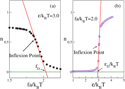
Figure 7: (a) Plot of the ’order parameter’, $n$, against pulling force $f$, for an adsorption strength $\varepsilon/k_{B}T=3.0$. The polymer chain length is $N$=128. The tangent at the inflexion point of the curve meets the abscissa at $f_{D}$ which we define as the detachment force. (b) The ’order parameter’, $n$, against the adsorption potential $\epsilon$ for fixed pulling force $f=2.0$. The tangent at the inflexion point of the curve meets the abscissa at $\varepsilon_{D}/k_{B}T$ where the polymer adsorbs at the surface plane.

At constant surface potential, $\epsilon$, one finds that $n$ steeply decreases upon a small increase of the pulling force whereby the polymer chain undergoes a transition from an adsorbed phase to a grafted-detached state. In order to locate the point of chain detachment, we draw a tangent at the inflexion point of the curve $n$ vs. $f$. The detachment force, $f_{D}$, is then identified as the point where the tangent intersects the abscissa ($f$-axis) - see Fig. 7(a). Thus one can determine the detachment force as a function of the adsorption potential $\epsilon$. Alternately, from the plot of $n$ against the adsorption potential $\epsilon$, with the pulling force $f$ held constant, one can observe that as sharp growth of $n$ as the potential is slightly increased. The critical potential for chain attachment at the transition point can be found similarly as indicated in Fig. 7(b).

Fig. 8(a) shows the variation of the order parameter with changing surface potential for several values of the pulling force. Evidently, the larger the pulling force, the stronger the surface potential, needed to keep the polymer adsorbed on the plane. In the absence of a force, the order paramenter changes smoothly. For larger forces, however, the transition becomes rapidly abrupt. This abrupt behavior of the order parameter is in close agreement with our theoretical predictions, depicted in Fig. 5. In Fig.  8(b) we show the variation of the order parameter $n$ with changing force $f$ for various adsorption potentials $\epsilon$. The threshold values for polymer desorption, $\epsilon_{D}(f)$ and $f_{D}(\epsilon)$, as obtained for chains of different length, are then extrapolated to obtain the corresponding values in the thermodynamic limit $\rightarrow\infty$.

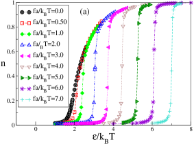
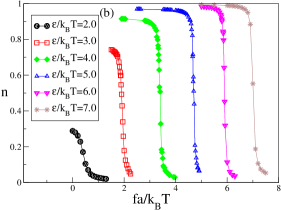
Figure 8: (a) The ’order parameter’, $n$, against the surface potential, $\epsilon$, for various pulling forces. The chain has length $N$=128. (b) Variation of $n$ with the pulling force, $f$, for several surface potentials.

Our observations show that $\epsilon_{D}$ increases slightly (i.e., the finite-size effects are rather small) with growing chain length $N$. By extrapolating the data to $1/N\rightarrow 0$ one obtains then $\epsilon_{D}$ for infinite length of the polymer chain. Similarly, the detachment force at fixed surface potential $\epsilon$ may be determined in the thermodynamic limit.

V.2 Adsorption-desorption phase diagram under pulling

Using the threshold values of $f_{D}$ and $\epsilon_{D}$ for critical adsorption/detachment in the thermodynamic limit, one can construct the adsorption-desorption phase diagram for a polymer chain. The phase diagram may be obtained by any of the two methods, i.e., (i) by fixing of the force and locating $\epsilon_{D}$, and/or (ii), by fixing of the surface potential and locating the detachment force $f_{D}$). The resulting phase diagram is displayed in Figure 9. The inset in Fig 9 shows that $f_{D}\propto(\epsilon-\epsilon_{c})^{0.97}$ which may be compared to the theoretical prediction $f_{D}\sim(\epsilon-\epsilon_{c})^{\nu/\phi}$. Hence, this method gives us an estimate for the crossover exponent $\phi$. For $\epsilon_{c}=1.67$ , we find $\phi\sim 0.59\pm 0.02$.

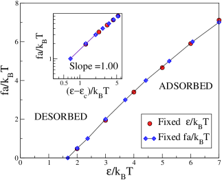
Figure 9: Plot of the critical detachment force $f_{D}$ against the surface potential $\epsilon$. In the inset in a double logarithmic plot $f_{D}$ is plotted against $(\epsilon-\epsilon_{c})/k_{B}T$. The critical adsorption potential for zero force has been found earlier Bhatt_stat_ads to be $\epsilon_{c}=1.67$.

V.3 Average lengths of loops and tails

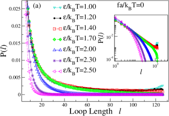
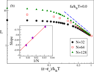
Figure 10: (a) Distribution of loop sizes for chain length $N=128$ at different strength of the surface potential and no pulling force. The inset shows the same in double logarithmic coordinates. The measured slope at $\epsilon_{c}/k_{B}T=1.67$ (full line) is $-1.38\pm 0.02$ which practically coincides with the prediction Eq.(18). (b) The average loop length plotted against $(\epsilon-\epsilon_{c})/k_{B}T$ where $\epsilon_{c}/k_{B}T=1.67$, for various chain lengths in double logarithmic coordinates. The slopes $x$, indicated by a dashed line, are obtained from the $L$ vs. $(\epsilon-\epsilon_{c})/k_{B}T$ curves, and plotted against $1/N$ in the inset. Extrapolation to $1/N\rightarrow 0$ yields $x\approx 0.95$.

In Fig 10a we plot the PDF of the loop sizes for a chain with $N=128$ at several strengths of the adsorption potential $\epsilon$ in the absence of pulling. One may readily verify that the PDF has a peak for loops of size unity which suggests that most frequently single-segment defects (that is, vacancies in the monomer trains) occur in the conformation of adsorbed chain. However, for $\epsilon<\epsilon_{c}$ one may detect clearly in Fig 10a slight increase in the distribution for loops of size $l\approx N$ which becomes more pronounced at smaller $\epsilon\approx 1.0\div 1.2$ in full agreement with the double-peaked shape, predicted by Eq. (25).

The average loop size $L$ is plotted against the surface potential (with regard to its critical value at the adsorption point), $(\epsilon-\epsilon_{c})/k_{B}T$ in Fig 10b. We find that, well inside the region of adsorption, $L$ scales as a power law, $L\propto(\epsilon-\epsilon)^{x}$. The exponent $x$, plotted as a function of $N$ in the inset, is negative, therefore, stronger attraction makes the loops smaller while the mean loop size evidently increases with growing chain length $N$ which is a finite size effect. The exponent $x$ approaches $-0.96$ in the limit $1/N\rightarrow 0$ - see inset in Fig 10b. This provides another estimate of the crossover exponent $\phi$ since $x=1-1/\phi$, according to Eq.(27). Thus we find $\phi\approx 0.51\pm 0.02$. From Fig 10b it is evident that the slope of the $L$ vs. $(\epsilon-\epsilon)/k_{B}T$ curves visibly changes as one comes closer to the CAP. In the immediate vicinity of $\epsilon_{c}$ the slope is small and the corresponding estimate for the crossover exponent in this region is $\phi\approx 0.63$. One should bear in mind, however, that this is due to the finite length of the chains used in the simulation which limits the possibility for the loop size to grow indefinitely, especially at $\epsilon_{c}$. Therefore, we use and depict measurements of the slope sufficiently far from the CAP where it tends to a constant value, indicated by the dashed line in Fig 10b.

In Fig. 11(a) we plot the PDF of the tail size for a chain with $N=128$ at several strengths of the adsorption potential in the absence of pulling. An interesting feature of the tail distribution function for $\epsilon=1.70$ immediately at the CAP, $\epsilon_{c}=1.67$, is the observed bimodal character. It means that there are two dominating chain populations, one with few loops and a long tail, and the other with many loops and a very short tail. Our simulation result thus confirms the shape of the tail distribution at criticality, Eq. (24), and appears in excellent agreement with the analytic result, derived earlier by Gorbunov et al. Gorbunov , indicating that in the vicinity of the critical adsorption point (CAP) chain conformations are either loop- or tail-dominated.

In Fig 11(b) the average tail length, $S$, is plotted against $(\epsilon-\epsilon_{c})/k_{B}T$. Again, $S$ is found to scale as a power law with the adhesion strength, $S\propto(\epsilon-\epsilon_{c})^{y}$ where $y$ is negative, decreases with $N$, and approaches eventually $-1.67$ for $1/N\rightarrow 0$ . This result can be compared to Eq.( 30). The corresponding estimate of $\phi$ is thus $0.60$.

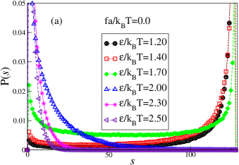
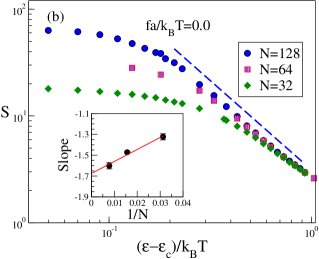
Figure 11: (a)Distribution of the tail size for different surface potentials in a polymer of length $N=128$ with no pulling force. (b) The average tail length $S$ against $(\epsilon-\epsilon_{c})/k_{B}T$ plotted for various chain lengths in double logarithmic coordinates. The slopes obtained from these curves are plotted against $1/N$ in the inset and extrapolated to get the thermodynamic limit $N\rightarrow\infty$.

We turn now to the properties of adsorbed chains in the presence of pulling force. A remarkable feature of the probability distribution of the order

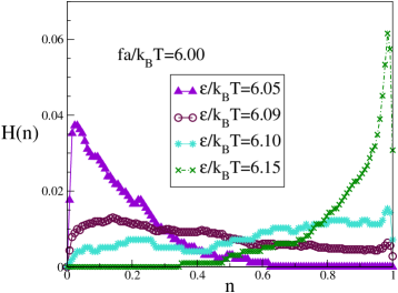
Figure 12: Distribution of the order parameter $n$ for a pulling force $fa/k_{B}T=6.0$ and different strength of adhesion $\epsilon/k_{B}T$. The chain length is $N=128$ and the threshold value of the surface potential for this force is $\epsilon_{D}\approx 6.095\pm 0.03$. The values $\epsilon/k_{B}T=6.09$ and $\epsilon/k_{B}T=6.10$ are on both sides of the detachment line, cf. Fig. 9.

parameter is the absence of a second peak in the vicinity of the critical strength of adsorption, $\epsilon_{D}\approx 6.095\pm 0.03$, which still keeps the polymer adsorbed at pulling force $fa/k_{B}T=6.0$, see Fig. 12. Somewhat further away from $\epsilon_{D}$, one observes a clear maximum in the distribution $H(n)$, indicating a desorbed chain with $n\approx 0.01$ for $\epsilon=6.05$, or an almost entirely adsorbed chain with $n\approx 0.99$ for $\epsilon=6.15$. This lack of bimodality in the $H(n)$ confirms the dichotomic nature of the desorption transition which rules out phase coexistence.

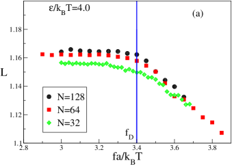
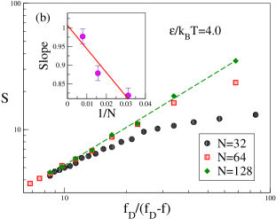
Figure 13: (a) The average loop length plotted against the pulling force $f$ for fixed $\epsilon/k_{B}T=4.0$. (b) The average tail length $S$ is plotted against the $(f-f_{D})^{-1}$ for various chain lengths for $\epsilon/k_{B}T=4.0$ in double logarithmic coordinates. The inset shows the extrapolated slope for $N\rightarrow\infty$ go to unity, as predicted by Eq. (73)

.

In Fig 13a, the average loop length, $L$ is plotted against the external pulling force $f$ for $\epsilon/k_{B}T=4.0$. For $f$ below the detachment threshold, $f_{D}$, the average loop size appears to be constant independent of the force. As the force $f$ exceeds $f_{D}$, the average loop size decreases in close agreement with the theoretical prediction, shown in Fig. 5a.

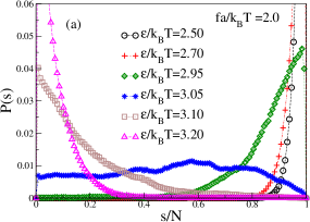
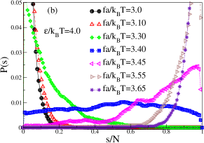
Figure 14: (a) Distribution of the tail size for a pulling force $fa/k_{B}T=2.0$ and different strength of adhesion $\epsilon/k_{B}T$. The chain length is $N=128$. (b) Distribution of the tail size for different force $f$ at $\epsilon/k_{B}T=4.0$.

In Fig 13b, the average tail length, $S$, is plotted against the difference $f_{D}-f$ for several chain lengths at surface adhesion $\epsilon/k_{B}T=4.0$ in double logarithmic coordinates. As the applied pulling force $f$ gradually approaches the threshold force for detachment, $f_{D}$, the tail gets systematically longer and comes close to the length of the chain $N$. Evidently, if one takes into account the finite-size effects which lead to the observed bending of $S\approx N$ at stronger pulling, the tail $S$ scales as $(f_{D}-f)^{-w}$. The exponent $w$ approaches $1.01$ (see inset in Fig 13b) at $\epsilon/k_{B}T=4.0$. This may be compared to the theoretical prediction of Eq. (73) which predicts indeed $w=1$.

Eventually, in Fig 14(a) the PDF of the tail size $s$ is plotted at different strengths of the surface potential $\epsilon$ while the force, applied to the chain end, is held constant, $f=2.0$. In contrast, in Fig 14(b), we display the distribution of tail size $s$ for the case when the adhesion strength is fixed, $\epsilon/k_{B}T=4.0$, whereas the pulling force $f$ is varied. Both graphs are remarkable in that they reflect the transition from fully adsorbed polymer, characterized by a sharp peak in the PDF at vanishing tail sizes, to detached chain when the pulling force exceeds the threshold $f_{D}$ and the corresponding PDF is peaked at $s/N\approx 1$. We emphasize again that although this phase transition of chain detachment is clearly of first order, no trace of a bimodal distribution in the vicinity of the transition line can be detected! Thus, the states on both sides of the phase boundary $f_{D}(\epsilon)$ cannot coexist simultaneously which underlines the peculiar nature of this phase transformation. At this point we should like to point out, however, that this exotic feature of the detachment transitions has meanwhile been established also in the case of the so called escape transition of a polymer coil, deformed under the tip of an Atomic Force Microscope Sub ; Yamakov . It has been shown rigirously recentlyKlushin , that despite its first order nature, the escape transition takes place without phase coexistence. Most probably, this unusual feature is due to the topological connectivity of polymer chain as quasi-onedimensional systems.

VI Summary and Discussion

In the present investigation we have studied the force-induced desoption transition of a polymer chain in contact with an adhesive surface. We treat the problem within the framework of the Grand Canonical Ensemble approach and derive analytic expressions for the various conformational building blocks, characterizing the structure of an adsorbed linear polymer chain, subject to pulling force of fixed strength. Closed analytic expressions for the fraction of adsorbed segments (i.e., the order parameter of the desorption transition) and for probability distributions of trains, loops and tails have been derived along with expressions for the corresponding first moments in terms of the surface potential intensity both with and without external force. As expected, all these conformational properties and their variation with the proximity to the CAP are governed by a crossover exponent $\phi$.

A central result in the present work is the calculation of $\phi$ using the approach of Kafri et al. Kafri which provides insight into the background of the existing controversial reports about its numeric value. We demonstrate that the value of $\phi$ may vary within the interval $0.39\leq\phi\leq 0.6$, depending on the possibility of a single loop to interact with the neighboring loops in the adsorbed polymer. Since this range is model-dependent, one should not be surprised that different models produce different estimates of $\phi$ in this interval.

A comparison with the results from extensive Monte Carlo simulations demonstrates the good agreement between theoretic predictions and simulation data.

In particular, we verify the gradual transition of the PDF of loops from power-law to exponential decay as one moves away from the critical adsorption point to stronger adsorption. We demonstrate that for vanishing pulling force, $f\rightarrow 0$, the mean loop size, $L\propto(\epsilon-\epsilon_{c})^{1-\frac{1}{\phi}}$, and the mean tail size, $S\propto(\epsilon-\epsilon_{c})^{\frac{1}{\phi}}$, diverge when one comes close to the CAP. In contrast, for a non-zero pulling force, $f\neq 0$, we show that the loops on the average get smaller with growing force while close to the detachment threshold, $f\approx f_{D}$, the tail length diverges as $S\propto(1-\frac{f}{f_{D}})^{-1}$.

Eventually, we derive the overall phase diagram of the force-induced desorption transition for a linear self-avoiding polymer chain and demonstrate its reentrant character when plotted in terms of detachment force $f_{D}$ against system temperature $T$. We find that despite being of first order, the force-induced phase transition of polymer desorption is dichotomic in its nature, that is, no phase coexistence and no metastable states exist. This unusual feature of the phase transformation is unambiguously supported by our simulation data, e.g., through the comparison of the order parameter probability distributions on both sides in the immediate vicinity of the detachment line whereby no double-peaked structure is detected.

Finally, we should like to to emphasize that while the present investigation will hopefully shed new light on the force-induced desorption transition of a linear polymer from a sticky surface, a lot more work is needed before a comprehensive understanding of this phenomenon is achieved. In this work simulations have been carried out within the framework of a constant force ensemble. In their comprehensive treatment of the problem, however, Skvortsov et al. SKB have shown that one may well work in the constant height ensemble whereby one uses the end-monomer $h$-position as an independent parameter and measures the force, exerted by the chain on the end monomer. Notwithstanding the equivalence of both ensembles, some quantities behave differently in each ensemble and this becomes evident only if one presents the salient features of the system behavior in each particular ensemble. Thus in the fixed-height ensemble, a different and rather interesting thermodynamic behavior of the measured mean detachment force and of the fraction of adsorbed segments agains $h$ is expected to be observed. Typically one then observes a constant force plateau while the height of the chain end monomer is varied. Such a behavior can be inferred even within the fixed-force ensemble. Indeed, as shown in Fig. 14b the PDF $P(s)$ is practically flat for the critical detachment force $f_{D}=3.40$, meaning that all chain end heights are equally probable at this particular force. The latter is equivalent to a constant-force plateau in the fixed-height ensemble. A verification by computer experiment is among our tasks in the immediate future as well as a study of the so far unexplored kinetics of chain detachment.

VII Acknowledgments

We are indebted to A. Skvortsov, L. Klushin, J.-U. Sommer, and K. Binder for useful discussions during the preparation of this work. A. Milchev thanks the Max-Planck Institute for Polymer Research in Mainz, Germany, for hospitality during his visit in the institute. A. Milchev and V. Rostiashvili acknowledge support from the Deutsche Forschungsgemeinschaft (DFG), grant No. SFB 625/B4.

Appendix A Properties of the polylog function

The polylog function $\Phi(\alpha,z)$ is defined by the series

$$\Phi(\alpha,z)=\sum_{k=1}^{\infty}\>\frac{1}{k^{\alpha}}\;z^{k}$$ (82)

which converges at $|z|<1$. From the definition, Eq. (82), one immediately obtains

$$z\>\frac{d}{dz}\>\Phi(\alpha,z)=\Phi(\alpha-1,z)$$ (83)

The calculation of the series Eq. (82) (see Sec. 1.11 in ref. Erdelyi ) gives

$$\Phi(\alpha,z)=\Gamma(1-\alpha)\left[\ln\left(\frac{1}{z}\right)\right]^{\alpha-1}+\sum_{r=0}^{\infty}\>\zeta(\alpha-r)\frac{(\ln z)^{r}}{r!}$$ (84)

where $\Gamma(x)$ is the gamma-function, $\zeta(x)$ is the Riemann zeta-function, and the exponent $\alpha$ is noninteger, i.e. $\alpha\neq 1,2,3,\dots$

Consider now the case of integer values of $\alpha$. The gumma-function $\Gamma(x)$ has poles at all negative integer arguments whereas the pole of $\zeta(x)$ is placed at $x=1$. One may write $\alpha=m+\delta$ where $m$ is a positive integer and $\delta\rightarrow 0$. Then in the vicinity of the poles the gamma- and zeta-functions can be rewritten as

$$\Gamma(1-m-\delta) = \frac{(-1)^{m}}{(m-1)!}\>\left[\frac{1}{\delta}-\psi(m)+{\cal O}(\delta)\right]$$

$$\zeta(1+\delta) = \left[\frac{1}{\delta}-\psi(1)+{\cal O}(\delta)\right]$$ (85)

where $\psi(x)$ is the digamma function (or $\psi$-function) defined as the logarithmic derivative of the gamma-function, $\psi(x)=d\ln\Gamma(x)/dx$. One should also take into account that

$$\left[\ln\left(\frac{1}{z}\right)\right]^{\delta}=1+\delta\ln\left[\ln\left(\frac{1}{z}\right)\right]+{\cal O}(\delta)$$ (86)

After taking into account Eqs.(85) and (86) in Eq. (84) and due to the cancellation of poles in the gamma- and zeta-functions at small values of $\delta$ the polylog function, Eq.(82) becomes Erdelyi

$$\Phi(m,z)=\frac{(\ln z)^{m-1}}{(m-1)!}\>\left[\psi(m)-\psi(1)-\ln\ln\left(\frac{1}{z}\right)\right]+\mathop{{\sum}^{\prime}}\limits_{r=0}^{\infty}\>\zeta(m-r)\;\frac{(\ln z))^{r}}{r!}$$ (87)

where the prime indicates that the term $r=m-1$ is to be omitted.

We are interested in the behavior of $\Phi(\alpha,z)$ at $z\rightarrow 1$. In this case $\ln(1/z)=-\ln[1-(1-z)]\approx(1-z)$. At $\alpha<1$, the main contribution comes from the first term in Eq. (84), i.e.

$$\Phi(\alpha,z)\approx\frac{\Gamma(1-\alpha)}{(1-z)^{1-\alpha}}$$ (88)

At $\alpha=1$ and $z\rightarrow 1$, and making use of Eq. (87), one obtains

$$\Phi(1,z)\approx-\ln\ln\left(\frac{1}{z}\right)\approx\ln\left(\frac{1}{1-z}\right)$$ (89)

Finally, at $\alpha>1$ the polylog function $\Phi(\alpha,z)$ has no singularity at $z\rightarrow 1$ and Eq.(84) results in the following expansion

$$\Phi(\alpha,z)\approx\zeta(\alpha)+\Gamma(1-\alpha)(1-z)^{\alpha-1}-\zeta(\alpha-1)(1-z)+\dots$$ (90)

In a bit more specific case when $1<\alpha<2$ we will use the well known relationship $\Gamma(1-\alpha)=-\pi/[\Gamma(\alpha)|\sin(\pi\alpha)|]$ so that

$$\Phi(\alpha,z)\approx\zeta(\alpha)-\frac{\pi}{\Gamma(\alpha)|\sin(\pi\alpha)|}(1-z)^{\alpha-1}-\zeta(\alpha-1)(1-z)+\dots$$ (91)

Taking into account the Eqs.(88), (89) and (91), the expression for the polylog function at $z\rightarrow 1$ reads

$$\Phi(\alpha,z)\approx\begin{cases}\frac{\Gamma(1-\alpha)}{(1-z)^{1-\alpha}},\quad&\mbox{\rm at}\quad\alpha<1\\ \\ \ln\left(\frac{1}{1-z}\right),\quad&\mbox{\rm at}\quad\alpha=1\\ \\ \zeta(\alpha)-a_{\alpha}(1-z)^{\alpha-1}-b_{\alpha}(1-z)+\dots,\quad&\mbox{\rm at}\quad 1<\alpha<2\end{cases}$$ (92)

where the coefficients $a_{\alpha}=\pi/{\Gamma(\alpha)|\sin(\pi\alpha)|}$ and $b_{\alpha}=\zeta(\alpha-1)$.

References

- (1) T. Strick, J.-F. Allemand, V. Croquette, and D. Bensimon, Phys. Today, 54, 46(2001).
- (2) F. Celestini, T. Frisch, and X. Oyharcabal, Phys. Rev. 70, 012801(2008).
- (3) H. G. Hansma, J. Vacuum Sci. Technol. B, 14, 1390(1995).
- (4) H. Kikuchi, N. Yokoyama, and T. Kajiyama, Chem. Lett. 11, 1107 (1997).
- (5) M. Rief, F. Oersterhelt, B. Heymann, and H. E. Gaub, Science, 275, 1295 (1997).
- (6) A. Kishino and T. Yanagida, Nature (London), 34, 74 (1998).,
- (7) S. B. Smith, Y. Cui, and C. Bustamante, Science, 271, 795 (1996).
- (8) K. Sviboda and S. M. Block, Annu. Rev. Biophys. Biomol. Struct., 23, 247 (1994).
- (9) A. Ashkin, Proc. Natl. Acad. Sci. USA, 94, 4853 (1997).
- (10) B. J. Haupt, J. Ennis, and E. M. Sevick, Langmuir, 15, 3868 (1999).
- (11) F. Hanke, L. Livadaru, and H. J. Kreuzer, Europhys. Lett. 69, 242 (2005).
- (12) A. Serr and R. R. Netz, Europhys. Lett. 73, 292 (2006).
- (13) A. M. Skvortsov, L. I. Klushin, and T. M. Birshtein, Polymer Sci. A (Moscow) (2008) in press.
- (14) C.A. Hoeve, E.A. Di Marzio, P. Peyser, J. Chem. Phys. 42, 2558 (1965).
- (15) Y. Kafri, D. Mukamel, L. Peliti, Eur. Phys. J. B 27, 135 (2002).
- (16) D. Poland, H.A. Scheraga, J. Chem. Phys. 45, 1456 (1966); J. Chem. Phys. 45, 1469 (1966).
- (17) T. M. Birshtein, Macromolecules, 12, 715(1979); ibid. 16, 45(1983).
- (18) B. Duplantier, J. Stat. Phys. 54, 581 (1989).
- (19) C. Vanderzande, Lattice Model of Polymers, Cambridge University Press, Cambridge, 1998.
- (20) J.A. Rudnick, G.D. Gaspari, Elements of the random walk: an introduction for advanced students and researchers, Cambridge University Press, Cambridge, 2004.
- (21) A. Erdélyi, Higher transcendental functions, v.1, N.Y., 1953.
- (22) P.-G. de Gennes, C.R. Acad. Sci., Paris, II 294, 1317 (1982).
- (23) E. Bouchaud, M. Daud, J. Phys. A 20, 1463 (1987).
- (24) A. A. Gorbunov, A. M. Skvortsov, J. van Male, and G. J. Fleer, J. Chem. Phys. 114, 5366 (2001).
- (25) E. Eisenriegler, K. Kremer, K. Binder, J. Chem. Phys. 77, 6296 (1982).
- (26) R. Descas, J.-U. Sommer, A. Blumen, J. Chem. Phys. 120, 8831 (2004).
- (27) H. Meirovitch, S. Livne, J. Chem. Phys. 88, 4507 (1988).
- (28) R. Hegger, P. Grassberger, J. Phys.A 27, 4069 (1994).
- (29) P. Grassberger, J. Phys.A 38, 323 (2005).
- (30) S. Metzger, M. Müller, K. Binder, J. Baschnagel, Macromol. Theory Simul. 11, 985 (2002).
- (31) H.-W. Diehl, S. Dietrich, Phys. Rev. B 24, 2878 (1981).
- (32) H.-W. Diehl,Phase Transition and Critical Phenomena, v. 10, ed. C. Domb and J.L. Lebowitz (N.Y., Academic), 1986.
- (33) E. Eisenriegler,Polymers Near Surfaces, Wold Scientific, London, 1993.
- (34) H.-W. Diehl, M. Shpot, Phys. Rev. Lett. 73, 3431 (1994).
- (35) H.-W. Diehl, M. Shpot, Nucl. Phys. B 528, 595 (1998).
- (36) A.A. Gorbunov, A.M. Skvortsov, J. Chem. Phys. 98, 5961 (1993).
- (37) A.M. Skvortsov, A.A. Gorbunov, L.I. Klushin, J. Chem. Phys. 100, 2325 (1994).
- (38) T. Kreer, S. Metzger, M. Müller, K. Binder, J. Baschnagel, J. Chem. Phys. 120, 4012 (2004).
- (39) S. Bhattacharya, H.-P. Hsu, A. Milchev, V. G. Rostiashvili, and T. A. Vilgis, Macromolecules, 41, 2920, (2008).
- (40) J. des Cloizeaux, G. Jannink, Polymers in Solution, Clarendon Press, Oxford, 1990.
- (41) P.-G. de Gennes, Scaling Concepts in Polymer Physics, Cornell University Press, Ithaca, 1979.
- (42) K. Binder, Rep. Prog. Phys. 50, 783 (1987).
- (43) D. Marenduzzo, A. Travato, A. Maritan, Phys. Rev. E 64, 031901 (2001).
- (44) E. Orlandini, S.M. Bhattacharjee, D. Marenduzzo, A. Maritan, F. Seno, J. Phys. A: Math. Gen. 34, L-751 (2001).
- (45) E.A. Mukamel, E.I. Shakhnovich, Phys. Rev. E 66, 032901 (2002).
- (46) P.K. Mishra, S. Kumar, Y. Singh, Europhys. Lett. 69, 102 (2005).
- (47) J. Krawczyk, T. Prellberg, A.L. Owczarek, A. Rechnitzer, J. Stat. Mech. P10004 (2004).
- (48) K. Binder and A. Milchev, J. Computer-Aided Material Design, 9, 33(2002)
- (49) G. Subramanian, D. R. M. Williams, and P. A. Pincus, Europhys. Lett. 29, 285(1995); Macromolecules 29, 4045(1996).
- (50) A. Milchev, V. Yamakov, and K. Binder, Phys. Chem. Chem. Phys. 1, 2083 (1999); Europhys. Lett. 47, 675(1999).
- (51) L. I. Klushin, A. M. Skvortsov, and F. A. M. Leermakers, Phys. Rev. E 69, 061101(2004); A. M. Skvortsov, L. I. Klushin, and F. A. M. Leermakers, Macromol. Symp. 237, 73(2006); J. Chem. Phys. 126, 024905(2007).