Non-Adiabatic Fluctuation in Measured Geometric Phase

Abstract

We study how the non-adiabatic effect causes the observable fluctuation in the “geometric phase” for a two-level system, which is defined as the experimentally measurable quantity in the adiabatic limit. From the Rabi’s exact solution to this model, we give a reasonable explanation to the experimental discovery of phase fluctuation in the superconducting circuit system [P. J. Leek, et al., Science 318, 1889 (2007)], which seemed to be regarded as the conventional experimental error.

Introduction.- It was discovered by I. I. Rabi Rabi37 that the non-adiabatic transition of a quantum system in a time-dependent magnetic field was subject to the sign of its magnetic momentum. The exact solution was first given in 1937, but its physical significance for the relative phase acquired under adiabatic evolution was not clarified until five decades later Berry84 . It was M. V. Berry who found that this phase might contain a geometric part, now called the Berry’s phase. Then the quantum adiabatic approximation theorem (QAAT) Messiah62 was reproved to naturally include the Berry’s phase Sun88a and generalized to deal with the non-adiabatic effects for many cases Sun88b ; Sun90a ; Sun90b ; Sun93 ; Sun95 . On the other hand, because of its geometric dependence, conditional geometric phase was proposed as an intrinsically fault-tolerant way of performing quantum computation Jonathan00 .

In this paper, associated with a recent experiment about phase fluctuation in the superconducting circuit system Leek07 , the above Rabi’s solution is used to study in details the non-adiabatic effects for a two-level system (TLS) in a harmonically rotated field (see Fig.1). This field can be realized with a microwave field perpendicular to the static magnetic field both applied to the system. With the phase of the microwave linearly varying with time, the Hamiltonian harmonically rotates in the parametric space.

Generally speaking, the Berry’s phase is always accompanied with the dynamical phase, and thus its pure effect can not be observed directly. However, we apply a $\pi$-pulse to the TLS so that the evolution is divided into two parts with both of them in the same path but in the opposite directions. In this case, the effect of the dynamical phase can be completely eliminated. This is the technique referred to spin echo technique Abragam61 . Thus, the pure geometric effect can be observed. And that may result in observable fluctuation of the measured geometric phase due to the Rabi’s non-adiabatic transitions.

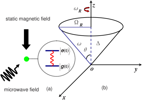
Figure 1: (color online) (a) Schematic diagram of a TLS in a static magnetic field along with a microwave field. (b) Realized effective Hamiltonian rotating in the parametric space.

Non-Adiabatic Effect with Berry’s Phase.-The evolution of the system can be well described with the Hamiltonian

$$H(t)=\frac{1}{2}(\Delta\sigma_{z}+\Omega_{R}\sigma_{x}\cos\omega_{R}t+\Omega_{R}\sigma_{y}\sin\omega_{R}t)\text{,}$$ (1)

where $\Delta$ is the energy splitting without the microwave field, $\Omega_{R}$ the Rabi frequency of the microwave, $\omega_{R}$ the oscillating frequency of the microwave’s phase, $\sigma_{x,y,z}$ the Pauli matrixes. Note that Hamiltonian (1) is exactly the effective Hamiltonian realized in Ref.Leek07 , where the rotating wave approximation Scully was applied. Straightforwardly, its instantaneous eigen states are obtained as

$$|e(t)\rangle =\cos\frac{\theta}{2}|0\rangle+\sin\frac{\theta}{2}e^{i\omega_{R}t}|1\rangle\text{,}$$ (2)

$$|g(t)\rangle =\sin\frac{\theta}{2}e^{-i\omega_{R}t}|0\rangle-\cos\frac{\theta}{2}|1\rangle\text{,}$$ (3)

with corresponding eigen energies $\pm\omega/2$. Here the energy splitting is $\omega=\sqrt{\Delta^{2}+\Omega_{R}^{2}}$, and the mixing angle is $\theta=\tan^{-1}(\Omega_{R}/\Delta)$. We also emphasize that due to the requirement of the single valueness of the eigenfunctions for a given Hamiltonian without singularity, the phase factor $\exp(\pm i\omega_{R}t)$ in $|e(t)\rangle$ or $|g(t)\rangle$ is fixed once the factor in the other state is chosen Shapere89 .

At time $t$, the evolution state is assumed to be a superposition $|\psi(t)\rangle=\alpha(t)|e(t)\rangle+\beta(t)|g(t)\rangle$ of two instantaneous eigen states . The time-dependent Schrödinger equation $H|\Psi(t)\rangle=i\partial_{t}|\Psi(t)\rangle$ leads to the following equations of coefficients

$$\dot{\alpha} =-i(\frac{\omega}{2}+\omega_{R}\sin^{2}\frac{\theta}{2})\alpha+i\beta^{\prime}\frac{\omega_{R}}{2}\sin\theta\text{,}$$ (4)

$$\dot{\beta^{\prime}} =i(\frac{\omega}{2}-\omega_{R}\cos^{2}\frac{\theta}{2})\beta^{\prime}+i\alpha\frac{\omega_{R}}{2}\sin\theta\text{,}$$ (5)

where $\beta^{\prime}(t)=\beta(t)\exp(-i\omega_{R}t)$.

Under the adiabatic conditions

$$\frac{\omega}{2}+\omega_{R}\sin^{2}(\frac{\theta}{2}) \gg\frac{\omega_{R}}{2}\sin\theta\text{,}$$ (6)

$$\frac{\omega}{2}-\omega_{R}\cos^{2}(\frac{\theta}{2}) \gg\frac{\omega_{R}}{2}\sin\theta\text{,}$$ (7)

the adiabatic approximate solutions to Eqs.(4) and (5) is obtained  by ignoring the terms with $\omega_{R}\sin\theta$ $/2$ . They show that both norms of the amplitudes remain the same as their initial values, while they acquire a Berry’s geometric phase $\pm\omega_{R}t(1-\cos\theta)/2$ in addition to the dynamical phase $\pm\omega t/2$ respectively.

On the other hand, the above Eqs.(4) and (5) can be solved exactly and it should be done so when the adiabatic condition is broken under certain circumstances. Thus, we have

$$\alpha =A_{1}e^{i\omega_{+}t}+A_{2}e^{i\omega_{-}t}\text{,}$$ (8)

$$\beta^{\prime} =B_{1}e^{i\omega_{+}t}+B_{2}e^{i\omega_{-}t}\text{,}$$ (9)

where $\omega_{\pm}=(-\omega_{R}\pm\Omega)/2\equiv(-\omega_{R}\pm\sqrt{\omega^{2}-2\omega\omega_{R}\cos\theta+\omega_{R}^{2}})/2$, and the coefficients are determined by the initial values $\alpha(0)$ and $\beta(0)$,

$$A_{1} =\frac{\beta(0)\omega_{R}\sin\theta+\alpha(0)(-\omega+\Sigma_{+})}{2\Omega}\text{,}$$

$$A_{2} =\frac{-\beta(0)\omega_{R}\sin\theta+\alpha(0)(\omega+\Sigma_{-})}{2\Omega}\text{,}$$

$$B_{1} =\frac{\beta(0)(\omega+\Sigma_{-})+\alpha(0)\omega_{R}\sin\theta}{2\Omega}\text{,}$$

$$B_{2} =\frac{\beta(0)(-\omega+\Sigma_{+})-\alpha(0)\omega_{R}\sin\theta}{2\Omega}\text{,}$$

where $\Sigma_{\pm}=\omega_{R}(1\pm\cos\theta)+2\omega_{+}.$

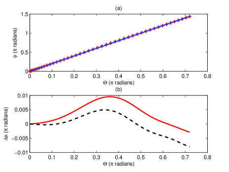
Figure 2: (color online) (a) Comparison between the Berry’s phase (blue solid line) $\phi_{B}$ and non-adiabatic phase (red cross) $\phi_{na}$ with $n=1$ circular rotation in each round. (b) The discrepancy between them with red solid line for the numerical result and black dashed line for the second order approximation.

Generally speaking, the Berry’s phase can not be observed directly from the experiment, since the dynamical phase always occurs along with the Berry’s phase. Here, we consider a concrete case where the total evolution is divided into two rounds, both of which are in the same path but with opposite directions. Provided that both the excited and the ground states acquire the same dynamical phase but with opposite signs in each round, the dynamical phase can be canceled when the amplitudes are exchanged after the first round of evolution. Thereafter, by experiencing the inverse rotation in the parametric space, the dynamical phase is canceled while the Berry’s phase is doubled since the latter depends on the sign of the angle velocity $\omega_{R}$ while the former does not. Excellent agreement may be expected with the Berry’s prediction

$$\phi_{B}=2\omega_{R}T(1-\cos\theta)$$ (10)

provided that the adiabatic condition, i.e., Eq.(6), is satisfied. Here, $T$ is the evolution time for each round.

However, when the non-adiabatic effect is considered, small deviation is expected. In Fig.(2), we plot the exact phase calculated from Eqs.(8) and (9), which is defined as the phase of $\alpha(2T)\beta^{\ast}(2T)$, denoted as

$$\phi_{na}=\text{angle}(\alpha(2T)\beta^{\ast}(2T))\text{.}$$ (11)

This is an observable quantity in experiment, which can be determined by measuring the complex amplitudes $\alpha(2T)$ and $\ \beta(2T).$ It just recovers the Berry’s phase in adiabatic limit.

It is predicted that the Berry’s phase is proportional to the solid angle $\Theta=2\pi(1-\cos\theta)$ subtended by the path. Recently, a measurement of the Berry’s phase in the superconducting qubit was carried out Leek07 . In order to compare the theoretical analysis with the experimental result, we adopt the same parameters as those given in Ref.Leek07 , i.e., $\Delta=50$ MHz, $\omega_{R}=(4n+1)$ MHz with $n$ being the number of loops. The tiny difference between those two can almost not be distinguished in Fig.(2a). Moreover, as shown in Fig.(2b), there are small oscillations in the deviation between them, $\Delta\phi=\phi_{na}-\phi_{B}$, with the root-mean-square deviation of $0.015$ rad from the expected lines while the counterpart for $n=1.5$ is $0.043$ rad. They are in reasonable agreement with the experimental result, i.e., $0.14$ rad Leek07 , considering that the rotating wave approximation Scully was applied to obtain the Hamiltonian (1) and the non-adiabatic effect in the process of applying the microwave field also accounted for part of the deviation.

Second-Order Fluctuation.-It was C. N. Yang who firstly pointed out that the Berry’s phase could be recovered from the original QAAT by retaining the first order term $O(\omega_{R}/\omega)$ in the phase. And this point of view was shortly confirmed by one (CPS) of the authors Sun95 using the Rabi’s exact solution. Here, with careful calculation to the second order term $O(\omega_{R}/\omega)^{2}$, the fluctuation in the phase is obtained. For an initial state with $\alpha(0)=\beta(0)=1/\sqrt{2}$, the measured deviation from the expected Berry’s phase is given as

$$\Delta\phi= \lambda^{2}(\sin\phi_{1}+4\sin\phi_{2}+2\sin\phi_{3}+2\sin\phi_{4}$$

$$+2\sin\phi_{5}+\sin\phi_{6}+2\sin\phi_{7}+\sin\phi_{8}$$

$$+2\sin\phi_{9}+2\sin\phi_{10}+4\sin\phi_{11}+4\sin\phi_{12})\text{,}$$ (12)

where $\lambda=\omega_{R}\sin\theta/2\omega$, $\phi_{j}=\phi_{j}^{\prime}-\phi_{B}$ ($j=1,2\ldots$) with

$$\phi_{1}^{\prime} =\pi-2T\omega_{R}\cos\theta\text{,}$$

$$\phi_{2}^{\prime} =-T\omega_{R}\text{,}$$

$$\phi_{3}^{\prime} =T\omega_{R}(-1+2\cos\theta)\text{,}$$

$$\phi_{4}^{\prime} =-\frac{T(\omega_{R}^{2}+8\omega_{R}\omega+4\omega^{2}-4\omega_{R}\omega\cos\theta-\omega_{R}^{2}\cos 2\theta)}{4\omega}\text{,}$$

$$\phi_{5}^{\prime} =\pi+\frac{T(-(\omega_{R}+2\omega)^{2}+4\omega_{R}\omega\cos\theta+\omega_{R}^{2}\cos 2\theta)}{4\omega}\text{,}$$

$$\phi_{6}^{\prime} =\pi+\frac{T((\omega_{R}-2\omega)^{2}-\omega_{R}^{2}\cos 2\theta)}{2\omega}\text{,}$$

$$\phi_{7}^{\prime} =\frac{T(\omega_{R}^{2}-2\omega_{R}\omega+4\omega^{2}-\omega_{R}^{2}\cos 2\theta)}{2\omega}\text{,}$$

$$\phi_{8}^{\prime} =\pi+\frac{T(\omega_{R}^{2}+4\omega^{2}-\omega_{R}^{2}\cos 2\theta)}{2\omega}\text{,}$$

$$\phi_{9}^{\prime} =\pi+\frac{T((\omega_{R}-2\omega)^{2}-4\omega_{R}\omega\cos\theta-\omega_{R}^{2}\cos 2\theta)}{4\omega}\text{,}$$

$$\phi_{10}^{\prime} =\frac{T(\omega_{R}^{2}+4\omega^{2}-4\omega_{R}\omega\cos\theta-\omega_{R}^{2}\cos 2\theta)}{4\omega}\text{,}$$

$$\phi_{11}^{\prime} =\frac{T(\omega_{R}^{2}-8\omega_{R}\omega+4\omega^{2}+4\omega_{R}\omega\cos\theta-\omega_{R}^{2}\cos 2\theta)}{4\omega}\text{,}$$

$$\phi_{12}^{\prime} =\pi+\frac{T((\omega_{R}-2\omega)^{2}+4\omega_{R}\omega\cos\theta-\omega_{R}^{2}\cos 2\theta)}{4\omega}\text{.}$$

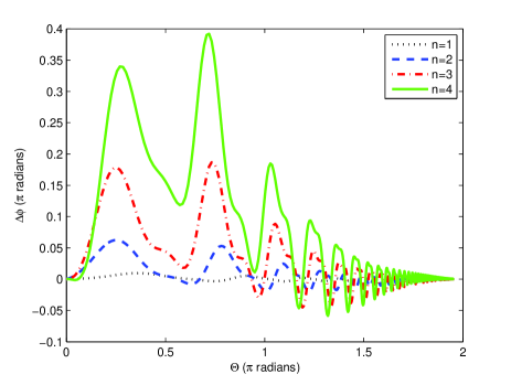
Figure 3: (color online) Comparison between different numbers of rotation loops $n$, with black dotted line for $n=1$, blue dashed line for $n=2$, red dash-dot line for $n=3$ and green solid line for $n=4$.

It can be seen from Eq.(12) that the sinusoidal deviation from the expectation will be present in the measured phase. As shown in Fig.2(b), the behavior is well described by the second order approximation. Although there is small distinction between it and the exact result, it is believed that it is due to the higher order terms. Based on the above theoretical analysis, we may safely arrive at the conclusion that due to the non-adiabatic evolution of the TLS, not only do the relative phases of the amplitudes of the two states change with time, but also do their norms. In other words, the non-adiabatic transition results in the small fluctuation of the measured phase.

To further explore the non-adiabatic effect, we investigate the phase fluctuation for different rotation velocity $\omega_{R}$’s. In Fig.3, the discrepancy between the measured phase and the Berry’s phase is plotted. As expected from Eq.(12), the sinusoidal oscillation is again witnessed. Additionally, the oscillating amplitudes rise as the rotating velocity is increased. Here, the total time for evolution is fixed AboutTime . This result is consistent with Eq.(12) as $\Delta\phi$ scales as $\omega_{R}^{2}$. Notice that all of them nonexceptionally approach zero at the both ends. It is a reasonable result since $\Delta\phi$ vanishes as $\theta=0$. Actually, the Hamiltonian remains the same as its initial state in the parametric space. The only effect for time evolution is to acquire a dynamical phase. On the other hand, as $\theta$ approaches $\pi/2$,

$$\omega=\sqrt{\Omega_{R}^{2}+\Delta^{2}}>\Omega_{R}\gg\Delta>\omega_{R}$$

since $\Delta$ is fixed. Due to vanishing of $\lambda$, we have a zero deviation from the predicted phase, i.e., $\Delta\phi=0$. In the limit $\theta\rightarrow\pi/2$, the initial state $|\psi(0)\rangle=(|0\rangle+|1\rangle)/\sqrt{2}$ is the eigen state of the initial Hamiltonian $H(0)\simeq\Omega_{R}\sigma_{x}/2$. Intuitionally, the evolution of the system is similar to the situation that a classical magnetic moment initially parallel to the applied field closely follows the rotation of the field.

Conclusion.-In this paper, we have investigated the fluctuation in the phase due to the non-adiabatic evolution. In contrast to the adiabatic evolution, the sinusoidal deviation from the expected line drawn for the Berry’s phase is observed. The phase fluctuations discovered in the recent experiment can be partially explained by our theoretical analysis. For a given time of evolution, it is predicted that the fluctuation from the Berry’s prediction rises larger and larger as the number of loops is increased.

Acknowledgement.-One (QA) of the authors would be grateful for stimulating discussions with Y. S. Li and valuable comments on the manuscript from Z. Q. Yin. This work is partially supported by the National Fundamental Research Program Grant No. 2006CB921106, China National Natural Science Foundation Grant No. 10775076.

References

- (1) I. I. Rabi, Phys. Rev. 51, 652 (1937).
- (2) M. V. Berry, Proc. R. Soc. London Ser. A 392, 45 (1984).
- (3) A. Messiah, Quantum Mechanics (North-Holland, Amsterdam, 1962).
- (4) C. P. Sun, J. Phys. A 21, 1585 (1988).
- (5) C. P. Sun, Phys. Rev. D 38, 2908 (1988).
- (6) C. P. Sun, Phys. Rev. D 41, 1318 (1990).
- (7) C. P. Sun and M. L. Ge, Phys. Rev. D 41, 1349 (1990).
- (8) C. P. Sun, Phys. Scr. 48, 393 (1993).
- (9) C. P. Sun and L. Z. Zhang, Phys. Scr. 51, 16 (1995).
- (10) M. V. Berry, Proc. R. Soc. London Ser. A 414, 31 (1987).
- (11) J. A. Jones, V. Vedral, A. Ekert, and G. Castagnoli, Nature 403, 869 (2000).
- (12) A. Shapere, F. Wilczek, Geometric Phases in Physics (World Scientific, Singapore, 1989).
- (13) A. Abragam, Principles of Nuclear Magnetism (Oxford Univ. Press, Oxford, 1961).
- (14) P. J. Leek, J. M. Fink, A. Blais, R. Bianchetti, M. Göppl, J. M. Gambetta, D. I. Schuster, L. Frunzio, R. J. Schoelkopf, A. Wallraf, Science 318, 1889 (2007).
- (15) M. O. Scully, M. S. Zubairy, Quantum Optics, (Cambridge University Press, Cambridge, England, 1997).
- (16) In the experiment, the total time consisted of the evolution of two rotations and the processes of applying and removing the microwave field. For the sake of excluding the phase decoherence, the total time for evolution ns is fixed. In contrast, the time for each rotation varies with .