Ultracold Atomic Gases: Novel States of Matter

LUDWIG MATHEY^a, SHAN-WEN TSAI^b, and ANTONIO H. CASTRO NETO^c

^a Harvard University, Cambridge, Massachusetts, USA
^b University of California, Riverside, California, USA
^c Boston University, Boston, Massachusetts, USA

Glossary

Bose-Einstein Condensation (BEC)
Low temperature phase of systems of identical bosons, characterized by superfluidity.

Boson
Particles with integer spin $S=0,1,2,...$. Mediators of interactions, such as photons and gluons are bosons. Objects made of an even number of fermions are bosons: positroniun (electron + positron), meson (two quarks), ⁸⁷Rb (37 protons, 48 neutrons and 37 electrons), ⁷Li (3 protons, 4 neutrons, 3 electrons).

Cooper pairs
At low temperatures and for attractive interactions fermions form a superconducting state, in which fermions form pairs which condense.

Fermi surface
Since fermions obey Pauli’s exclusion principle, the ground state of $N$ non-interacting fermions in $d$-dimensions is the state with the $N$ lowest energy states occupied. In momentum space the last occupied state and the first unoccupied state define a surface of dimensions $d-1$, called the Fermi surface.

Fermion
Particles with half-odd integer spin $S=\frac{1}{2},\frac{3}{2},\frac{5}{2},...$. Examples include elementary particles such as electrons and quarks. Objects made of an odd number of fermions are also fermionic, such as protons, ⁴⁰K (19 protons, 21 neutrons, and 19 electrons), and ⁶Li (3 protons, 3 neutrons, and 3 electrons).

Laser Cooling
In a typical experimental setup, the atoms are cooled to the regime of $10^{2}\mu K$, by using pairs of counterpropagating laser beams that are slightly red-detuned below an atomic transition. Due to the Doppler effect the atoms can only absorb a photon if they travel towards the beam with a high velocity. From that process the atoms experience a recoil, which slows them down.

Evaporative Cooling
To slow the atoms down further, to the $\mu K$ regime, one applies radio frequency radiation that flips the internal state to a high-field seeking, i.e. non-trapped, state in such a way, that only atoms of high kinetic energy can escape. Due to thermalization, this leads to cooling of the remaining atomic ensemble.

Magnetic Trap
The atoms are trapped by applying a spatially inhomogeneous magnetic field. This field leads to an energy shift due to the Zeeman effect, which the atoms experience as an external potential, for large energy splittings of the magnetic levels. Different geometric designs are in use, such as the TOP trap, or the Ioffe-Pritchard trap.

Optical Lattice
Counterpropagating laser beams create a standing wave field, which the atoms experience as a periodic potential, due to the ac Stark shift. If the temperature and all energy scales are small compared to the energy splitting due the spatial confinemenent in each well, this system is well approximated by a Hubbard model, i.e. by taking into account nearest-neighbor hopping and on-site interaction.

Nesting
Fermi surface with portions that are parallel. The vector that connects different parallel portions is called the nesting vector $\vec{Q}$.

I. Definition of the Subject and Its Importance

The work presented in this article belongs to the recently emerging interface of atomic physics and condensed matter theory. One of the crucial connections between these fields is the fact that ultracold atom ensembles in optical lattices, i.e. periodic potentials provided by standing waves of laser light, are well described by Hubbard models, the quintessential model of many-body theory. Therefore, these experiments allow for the study of many-body effects in a well-defined and tunable environment.

The subject of this article is the study of quantum phases of ultracold atoms in optical lattices. The objective is to propose experimental configurations, such as what lattice geometry or which types of atoms to use, for which unusual many-body effects can be found. Besides the applicability to ultra-cold atom systems, and given the generic nature of the underlying models, the resulting phases are also of interest in solid state systems.

Using techniques such as a numerical implementation of functional renormalization group equations and Luttinger liquid theory, we find the phase diagrams of various low-dimensional systems of different geometry, and discuss how the various phases could be detected.

II. Introduction

The technology of cooling and trapping atomic ensembles has been one of the most important developments in physics over the last decades. It has been a critical ingredient in creating Bose-Einstein condensates [4, 14], improving atomic clocks [84], and studying atomic properties [60, 46]. A new direction in this development was the realization of the Mott insulator transition [30] with ultra-cold atoms, which demonstrated that these systems can be used to create various types of quantum phases in a tunable and well-defined environment. The subsequent progress that has been made in controlling and manipulating ensembles of ultra-cold atoms [97, 63, 64, 57], was followed by a number of experiments to create and study more and more sophisticated many-body effects, such as fermionic superfluids [31, 45, 114], one-dimensional strongly correlated Fermi and Bose systems [82, 52, 75], or noise correlations in interacting atomic systems [3, 66, 32, 21] . These developments established the notion of ’engineering’ many-body states in a tunable environment, i.e. manipulating ensembles of ultra-cold atoms in optical lattices.

This article further explores this development. The first step of creating novel states of matter is to determine the phase diagram of the system under consideration. For this purpose we use Luttinger liquid theory for studying one-dimensional quantum systems and two-dimensional thermal systems, and functional renormalization group equations to study two-dimensional quantum systems, which are both sophisticated methods that generate a lot of insight into the physics of these systems.

This article contains three main sections, which can be read independently of each other, organized as follows: in Section III we first study the phase diagram of an incommensurate Bose-Fermi mixture in one dimension, which can be understood as a Luttinger liquid of polarons (see [65, 69]). We then broaden the scope of this study to include the effects of commensurate densities (see [68]). In Section IV, we study the phases of two coupled two-dimensional superfluids, and we propose how the phase-locking transition of such systems can be used to realize the Kibble-Zurek mechanism, i.e. to create topological defects by ramping across a phase transition (see [71]). In Section V, we use a numerical implementation of functional renormalization group equations to study the phase diagrams of Bose-Fermi mixtures in optical lattices in two dimensions. For both a square and a triangular lattice we find a rich structure of competing phases (see [67, 70, 55]).

III. One-Dimensional Lattices

The theory of one-dimensional many-body systems has been a highly active and fascinating field of physics for many decades, the centerpiece of which is the notion of the Luttinger liquid [25, 27, 95]. In this section we propose several systems that display various features of Luttinger liquids, such as quasi-long range order, competing orders, and Kosterlitz-Thouless transitions due to commensurate densities, as will be explained.

Recent advances in controlling ultra cold atoms lead to the realization of truly one dimensional systems, and the study of many-body effects therein. Important benchmarks, such as the Tonks-Girardeau gas [82, 52] and the Mott transition in one dimension[97], have been achieved by trapping bosonic atoms in tight tubes formed by an optical lattice potential. Novel transport properties of one dimensional lattice bosons have been studied using these techniques[20]. More recently, a strongly interacting one dimensional Fermi gas was realized using similar trapping methods[75]. Interactions between the fermion atoms were controlled by tuning a Feshbach resonance in these experiments. On the theory side, numerous proposals were given for realizing a variety of different phases in ultra cold Fermi systems [88, 22, 10], Bose-Fermi mixtures[9, 65, 69, 93], as well as Bose-Bose mixtures[40, 41].

In the first part of this section, we describe the phase diagram of an incommensurate Bose-Fermi mixture, in the second part we consider the effect of commensurate fillings.

Luttinger liquid of polarons in one-dimensional Bose-Fermi mixtures

In this section we investigate one dimensional (1D) Bose-Fermi mixtures (BFM) using bosonization [35, 8]. The resulting quantum phases can be understood by introducing polarons, i.e. atoms of one species surrounded by screening clouds of the other species. In our analysis the polarons emerge as the most well-defined quasi-particles in the interacting system while quantum phases of the system arise from a competition of various ordering instabilities of such polarons. The phase diagrams we obtain show a remarkable similarity to the Luttinger liquid phase diagrams of 1D interacting electron systems [95, 47], suggesting that 1D BFM may be understood as Luttinger liquids of polarons.

To illustrate the results of this section, we show a typical phase diagram for a BFM in an optical lattice in Fig. 1, as a function of experimentally controlled parameters. We consider two types of atoms, one fermionic and one bosonic, moving in a lattice potential with the amplitude $V_{b,\|}$ (see [69]), and interacting via a short-ranged interaction characterized by the scattering length $a_{bf}$ between bosons and fermions. We use these parameters, the scattering length $a_{bf}$ and the strength of the longitudinal optical lattice for bosonic atoms ($V_{b,\|}$) [18], as tuning parameters in Fig. 1.

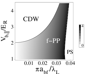
Figure 1: Phase diagram for a mixture of bosonic and spinless fermionic atoms in a 1D optical lattice. Shading in the $f$-PP phase describes the strength of the bosonic screening cloud ($2\lambda$, see Eq.(4)) around a pair of fermions. $\lambda_{L}$ and $E_{R}$ are respectively the lattice period and recoil energy. Other parameters used for this figure are (see text for notations, [69] for details): $\nu_{b}=4$, $\nu_{f}=0.5$, $V_{b,\perp}=V_{f,\perp}=20E_{R}$, $V_{f,\|}=2E_{R}$, boson-boson scattering length $a_{bb}=0.01\lambda_{L}$.

For relatively weak interactions and slow bosons (i.e. large $V_{b,\|}$) the system is in the charge-density-wave (CDW) phase, in which the densities of fermions and bosons have a periodic modulation [19]. For very strong interactions the system is unstable to phase separation (PS) [9, 1, 7]. The two regimes are separated by a $p$-wave pairing phase of fermionic polarons ($f$-PP). Our analysis is carried out for the most promising system of atoms in an optical lattice. However, qualitative results should also apply to atoms in a tight 1D cigar-shaped magnetic trap [26]. A sketch of the two phases is shown in Fig. 2.

The essence of the bosonization procedure is to diagonalize the effective low-energy Hamiltonian, which allows for the exact calculation of all relevant correlation functions. The phase diagrams are determined by finding the order parameter which has the most divergent susceptibility [95, 47]. Bosonization approach has been applied to BFM in Ref. [9]. However, that work did not consider the formation of polarons and, as a result, did not describe most of the quantum phases discussed here. The present system also has a close analogy to 1D electron-phonon systems discussed previously (see e.g. Ref. [107]). A qualitative difference of the electron-phonon system is that the sound velocity is usually much smaller than the Fermi velocity, whereas for a BFM the velocity of the phonon modes (of the bosonic condensate) can be larger than the Fermi velocity. We also note that the 1-D $p$-wave superfluid we obtain here may be of relevance to a recent proposal for quantum computation [53].

We now give an overview over the, somewhat technical, derivation of this phase diagram, before we discuss issues concerning the experimental realization and detection of these phases, and conclude. We consider a mixture of spinless fermionic ($f$) and bosonic ($b$) atoms. For a sufficiently strong optical potential the microscopic Hamiltonian is given by a single band Hubbard model

$$H = -\sum_{\langle ij\rangle}\left(t_{b}b_{i}^{\dagger}b_{j}+t_{f}f_{i}^{\dagger}f_{j}\right)-\sum_{i}\left(\mu_{f}n_{f,i}+\mu_{b}n_{b,i}\right)+\frac{U_{b}}{2}\sum_{i}n_{b,i}(n_{b,i}-1)+U_{bf}\sum_{i}n_{b,i}n_{f,i},$$ (1)

where $n_{b/f,i}$ are the boson/fermion density operators with $\mu_{b/f}$ being their chemical potentials. The tunneling amplitudes $t_{f/b}$, and the particle interactions $U_{b}$ and $U_{bf}$ can be expressed explicitly in terms of the $s$-wave scattering lengths, the laser beam intensities and atomic masses [42]. For simplicity we assume that the filling fraction of fermions $\nu_{f}\equiv\langle n_{f,i}\rangle$ is not commensurate with the lattice or with the filling fraction of bosons $\nu_{b}$. Therefore, we can neglect lattice-assisted backward/Umklapp scattering. The Fermi momentum and velocity are given by $k_{f}=\pi\nu_{f}$ and $v_{f}=2t_{f}\sin(k_{f})$, respectively.

In Haldane’s bosonization approach [35, 8] 1D fermion and boson operators can be represented by $f(x)=\left[\nu_{f}+\Pi_{f}\right]^{1/2}\sum_{m=-\infty}^{\infty}e^{(2m+1)i\Theta_{f}}e^{i\Phi_{f}}$ and $b(x)=\left[\nu_{b}+\Pi_{b}\right]^{1/2}\sum_{m=-\infty}^{\infty}e^{2mi\Theta_{b}}e^{i\Phi_{b}}$, where $x$ is a continuous coordinate that replaces the site index $i$. The operators $\Pi_{f/b}(x)$ and $\Phi_{f/b}(x)$ are the bosonized density and phase fluctuation operators. The $\Theta_{f/b}(x)$ fields are given by $\Theta_{f/b}\equiv\pi\nu_{f/b}x+\pi\int^{x}dy\Pi_{f/b}(y)$. The low-energy effective Hamiltonian thus can be written as:

$$H_{\rm eff} = \sum_{\alpha=b,f}\frac{v_{\alpha}}{2}\int dx\left[\frac{K_{\alpha}}{\pi}\left(\partial_{x}\Phi_{\alpha}\right)^{2}+\frac{\pi}{K_{\alpha}}\Pi_{\alpha}^{2}\right]+U_{bf}\int dx\Pi_{b}\Pi_{f}+\frac{2G}{2\pi}\int dx\left[\pi^{2}\Pi_{f}^{2}-(\partial_{x}\Phi_{f})^{2}\right].$$

where $v_{b}$ and $K_{b}$ are the phonon velocity and Luttinger exponent of the bosons and $K_{f}=1$ for noninteracting fermion atoms.

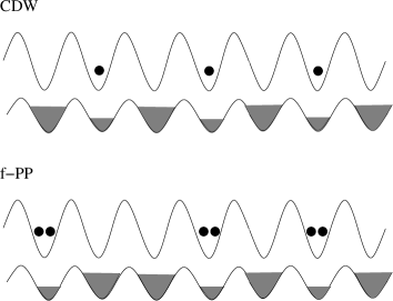
Figure 2: Illustration of the two phases that occur in a BFM with spinless fermions, CDW and $f$-PP. In the CDW phase the system develops a $2k_{f}$ density modulation in both the fermionic and the bosonic liquid. In the $f$-PP phase, the fermions form polarons, indicated by the reduced bosonic density in their vicinity, that is, their polarization cloud. This polarization leads to an effective attractive interaction, which causes these fermionic polarons to pair up and form a superfluid state.

To obtain the last term of $H_{\rm eff}$ we have integrated out the high energy ($2k_{f}$) phonons within the instaneous approximation (i.e. assuming $v_{b}\gg v_{f}$). $G\equiv\frac{g_{2k_{f}}^{2}}{\omega_{2k_{f}}}$, where $\omega_{k}$ is the (Bogoliubov) phonon energy dispersion [104] and $g_{k}=U_{bf}\sqrt{\nu_{b}\,\varepsilon_{b,k}/2\pi\omega_{k}}$ is the fermion-phonon (FP) coupling vertex with $\varepsilon_{b,k}$ being the noninteracting boson band energy. In the long wavelength limit we have a conventional FP coupling $g_{k}=g|k|^{1/2}$ with $g\equiv U_{bf}\sqrt{K_{b}}/2\pi$. The effective Hamiltonian, Eq. (LABEL:H_eff), is quadratic and can be diagonalized [17]. The resulting two eigenmode velocities are given by [9]

$$v_{a,A}^{2} = \frac{1}{2}(v_{b}^{2}+\tilde{v}_{f}^{2})\pm\frac{1}{2}\sqrt{(v_{b}^{2}-\tilde{v}_{f}^{2})^{2}+16\tilde{g}^{2}v_{b}\tilde{v}_{f}},$$ (3)

where $\tilde{v}_{f}\equiv(v_{f}^{2}-4G^{2})^{1/2}$ and $\tilde{g}\equiv g\,e^{\theta}$ with $e^{\theta}=((v_{f}-2G)/(v_{f}+2G))^{1/4}$. When the FP coupling $g$ becomes sufficiently strong the eigenmode velocity $v_{A}$ becomes imaginary, indicating an instability of the system. This instability corresponds to phase separation (global collapse) for positive (negative) $U_{bf}$[9].

To understand the nature of the many-body state of BFM outside of the instability region we analyze the long distance behavior of the correlation functions. For the bare bosonic and fermionic particles we find $\langle b(x)b^{\dagger}(0)\rangle\sim|x|^{-\frac{1}{2}K_{\epsilon}^{-1}}$ and $\langle f(x)f^{\dagger}(0)\rangle\sim\cos(k_{f}x)|x|^{-\frac{1}{2}(K_{\beta}+K_{\gamma}^{-1})}$ [15]. To describe particles dressed by the other species we introduce the composite operators

$$\tilde{f}(x)\equiv e^{-i\lambda\Phi_{b}(x)}f(x),\ \ \ \tilde{b}(x)\equiv e^{-i\eta\Phi_{f}(x)}b(x),$$ (4)

with $\lambda$ and $\eta$ being some real numbers. The correlation functions of these operators are given by $\langle\tilde{f}(x)\tilde{f}^{\dagger}(0)\rangle\sim\cos(k_{f}x)|x|^{-\frac{1}{2}(K_{\beta}+\lambda^{2}K_{\epsilon}^{-1}+K_{\gamma}^{-1}-2\lambda K_{\gamma\epsilon}^{-1})}$ and $\langle\tilde{b}(x)\tilde{b}^{\dagger}(0)\rangle\sim|x|^{-\frac{1}{2}(K_{\epsilon}^{-1}+\eta^{2}K_{\gamma}^{-1}-2\eta K_{\gamma\epsilon}^{-1})}$ [15]. We observe that the exponents of the correlation functions are maximized for $\lambda_{c}=K_{\epsilon}/K_{\gamma\epsilon}$ and $\eta_{c}=K_{\gamma}/K_{\gamma\epsilon}$. From now on we will use Eq. (4) with $\lambda_{c}$ and $\eta_{c}$ to construct polaronic particles. In the limit of weak interactions we have $\lambda_{c}\to U_{bf}/U_{b}$ and $\eta_{c}\to 2U_{bf}/\pi v_{b}$. This result can be understood by a simple density counting argument that a fermionic polaron ($f$-polaron) locally suppresses (enhances) a bosonic cloud by $\lambda_{c}$ particles, whereas a bosonic polaron ($b$-polaron) depletes (enhances) the fermionic system by $\eta_{c}$ atoms for positive (negative) $g$.

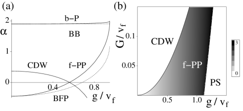
Figure 3: Ground state of a BFM with spinless fermions. (a) Scaling exponents of different order parameters (see the text). Parameters are chosen to be $v_{b}/v_{f}=3$, $K_{b}=5$ and $G/v_{f}=0.1$. (b) Global phase diagram for $v_{b}/v_{f}=5$ and $K_{b}=10$. Shading density indicates the strength of the screening clouds of a polaron pair, $2\lambda_{c}$.

The polaronic operators defined in Eq. (4) can also be introduced via the canonical polaron transformation (CPT), which is often used in polaron theory [62, 2]. The CPT operator is given by $U=e^{-i\lambda\sum_{{k}\neq 0}\left(F_{k}\beta_{k}\rho_{k}^{\dagger}+{\rm h.c.}\right)}$, where $\beta_{k}$ is the phonon annihilation operator, $\rho_{k}$ is the fermion density operator, $F_{k}$ is some function of wavevector $k$, and $\lambda$ specifies the strength of the phonon dressing. When applied to a fermion operator, the CPT transforms it to a polaron operator, $U^{-1}f(x)U=f(x)\exp\left[-i\lambda\sum_{{k}\neq 0}\left(F_{k}\beta_{k}e^{-i{k}\cdot{x}}+{\rm h.c.}\right)\right]$ [62, 2], which is the same as Eq.(4), provided that one takes $F_{k}=\sqrt{\frac{2\pi}{K_{b}|k|L}}{\rm sgn}(k)$. (Note that in 1D fermionic systems density operators correspond to Luttinger bosons.) We note, however, unlike in ordinary polaron theory, where further approximations after the CPT have to be made [62, 2], in the 1D BFM system we consider here, the full low energy quantum fluctuations have been included via bosonization method and exact diagonalization of the resulting Hamiltonian Eq. (LABEL:H_eff). This allows for an essentially exact determination of the polarization parameter $\lambda$.

Now we study the many-body ground state phase diagram of a 1D BFM, which is characterized by specifying the order parameters that have the slowest long distance decay of the correlation functions [95, 47]. Two types of ordering were found to occur: $2k_{f}$-ordering due to a Peierls-type instability and $f$-polaron pairing due to their effective attractive interactions induced by the screening clouds. For the $2k_{f}$ CDW order parameter, $O_{CDW}=f^{\dagger}_{L}f_{R}$, we find $\alpha_{CDW}=2-2K_{\beta}$, and for the $f$-polaron pairing field, $O_{f-PP}=\tilde{f}_{L}\tilde{f}_{R}$, we obtain $\alpha_{f-PP}=2-2\left[\lambda^{2}_{c}K_{\epsilon}^{-1}+K_{\gamma}^{-1}-2\lambda_{c}K_{\gamma\epsilon}^{-1}\right]$. We did not include polaron dressing in $O_{CDW}$, since this operator has no net fermionic charge and the exponent of $O_{CDW}$ does not change if we replace $f$ by $\tilde{f}$. Scaling exponents shown in Fig. 3(a) demonstrate that divergencies of the CDW and $f$-PP susceptibilities (corresponding to positive $\alpha$) are mutually exclusive and cover the entire phase diagram outside the PS regime. In the same figure, we also show the scaling exponents calculated for bare fermion pairing ($O_{BFP}=f_{L}f_{R}$), bare boson condensate ($O_{BB}=b$), and $b$-polaron condensate ($O_{b-P}=\tilde{b}$). It is easy to see that the polaronic order parameters always have larger exponents than their counterparts constructed with bare atoms, showing the stability of polaronic quasi-particle in a 1D BFM system. Moreover, the necessity to consider $f$-polaron pairing instead of bare fermion pairing is further supported by considering the stability of superfluidity: we introduce a single weak impurity potential in the 1D BFM and determine its relevance by a renormalization group (RG) calculation [48]. We find that the impurity potential is relevant within the CDW phase and irrelevant outside of it. This indicates that there should be a superfluid phase outside of the insulating CDW phase , which supports the existence of $f$-polaron pairing instead of bare fermion pairing according to Fig. 3(a).

In Fig. 3(b) we show a global phase diagram of a BFM considering the FP coupling ($g$) and effective fermion-fermion interaction ($G$) as independent variables. One can see that the polaronic effects and the associated pairing phase are important when FP coupling ($g$) is large, while the CDW phase dominates when the effective fermion interaction ($G$) is increased. This phase diagram is very similar to what one finds for spinless electrons in Luttinger liquid theory [95, 47], where CDW and pairing phase compete with each other in the whole phase diagram. Therefore one can introduce a Luttinger liquid of polarons to describe BFM in 1D systems. The phase diagram in terms of experimentally controlled parameters was shown in Fig. 1. When considering finite temperature effects in a realistic experiment, we note that the correlation function is cut-off by thermal correlation lengths, which are approximately given by $\xi\sim v_{f}/k_{B}T$. Therefore the zero temperature ground states should appear when $\xi>L$ with $L$ being the system size. This corresponds to a temperature regime of $1\%$ of the Fermi temperature for systems of approximately 100 sites in the longitudinal direction.

Several approaches can be used to detect the quantum phases discussed above. First, in the CDW phase the fermion density modulation will induce a $2k_{f}$ density wave in the boson field in addition to the zero momentum condensation so that the CDW phase can be observed as interference peaks at momentum $k=2k_{f}$ in a standard time-of-flight (TOF) measurement for bosons [19]. Secondly, the polaron pairing phase can be observed by measuring the noise correlation of fermions in a TOF experiment as proposed in Ref. [3]. Thirdly, a laser stirring experiment [77, 87] can be used to probe the phase transition between the insulating (pinned by trap potential) CDW and the superfluid $f$-PP phase: one can use a laser beam focused at the center of the cloud and stir such local potential to measure the response of the BFM. If the system is in the pairing phase, the laser beam can be moved through the system without dissipation if only its velocity is slower than some critical value [77, 87]. At the $f$-PP/CDW phase boundary this critical velocity goes to zero, reflecting a transition to the insulating (CDW) state. This scenario follows from the above described RG analysis of a single impurity potential [48]. Finally a way to probe the PS boundary could be to measure the dipolar collective oscillations of the system, generated by a sudden displacement of the harmonic trap potential with respect to the lattice potential [61, 24, 106]. When the system is near the PS boundary, fermion-boson interaction will strongly reduce the frequency of the dipolar mode.

In summary, we used bosonization to investigate the quantum phases of 1D mixtures of bosonic and fermionic atoms involving spinless fermions. The phase diagram that we found can be understood in terms of a Luttinger liquid of polarons. We also described several experimental techniques for probing these quantum phases.

Commensurate mixtures of ultra-cold atoms in one dimension

In this section we explore the behavior of ultracold atomic mixtures, confined to one-dimensional (1D) motion in an optical lattice, that exhibit different types of commensurability, by which we mean that the atomic densities and/or the inverse lattice spacing have an integer ratio. Commensurable fillings arise naturally in many ultracold atom systems, because the external trap potential approximately corresponds to a sweep of the chemical potential through the phase diagram, and therefore passes through points of commensurability. At these points the system can develop an energy gap, which fixes the density commensurability over a spatially extended volume. This was demonstrated in the celebrated Mott insulator experiment by Greiner et al.[30], where Mott phases with integer filling occurred in shell-shaped regions in the atom trap. These gapped phases gave rise to the well-known signature in the time-of-flight images[100], and triggered the endeavor of ‘engineering’ many-body states in optical lattices. Further examples include the recently created density-imbalanced fermion mixtures [83, 115] in which the development of a balanced, i.e. commensurate, mixture at the center of the trap is observed.

In 1D, this phenomenon is of particular importance, because it is the only effect that can lead to the opening of a gap, for a system with short-range interactions. In contrast to higher dimensional systems, where, for instance, pairing can lead to a state with an energy gap, in 1D only discrete symmetries can be broken, due to the importance of fluctuations. Orders that correspond to a continuous symmetry can, at most, develop quasi long range order (QLRO), which refers to a state in which an order parameter $O(x)$ has a correlation function with algebraic scaling, $\langle O(x)O(0)\rangle\sim|x|^{-(2-\alpha)}$, with a positive scaling exponent $\alpha$.

Due to its importance in solid state physics, the most thoroughly studied commensurate 1D system is the SU(2) symmetric system of spin-1/2 fermions. This system develops a spin gap for attractive interaction and remains gapless for repulsive interaction, as can be seen from a second order RG calculation. However, the assumed symmetry between the two internal spin states, which is natural in solid state systems, does not generically occur in Fermi-Fermi mixtures (FFMs) of ultra-cold atoms, where the ‘spin’ states are in fact different hyperfine states of the atoms. An analysis of the generic system is therefore highly called for. Furthermore, we will extend this analysis to both Bose-Fermi (BFMs) and Bose-Bose mixtures (BBMs), as well as to the dual commensurability, in which the charge field, and not the spin field, exhibits commensurate filling, as will be explained below.

The main results of this section are the phase diagrams shown in Fig. 4 and 5. We find that both attractive and repulsive interactions can open an energy gap. For FFMs the entire phase diagram is gapped, except for the repulsive SU(2) symmetric regime (cp. [10]), for BFMs or BBMs the bosonic liquid(s) need(s) to be close to the hardcore limit, otherwise the system remains gapless. Furthermore, we find a rich structure of quasi-phases, including charge and spin density wave order (CDW, SDW), singlet and triplet pairing (SS, TS), polaron pairing [65, 69], and a supersolid phase, which is the first example of a supersolid phase in 1D. These results are derived within a Luttinger liquid (LL) description, which treats bosonic and fermionic liquids on equal footing.

We will now classify the types of commensurability that can occur in a system with short-ranged density-density interaction. We consider Haldane’s representation [35, 8] of the densities for the two species:

$$n_{1/2} = [\nu_{1/2}+\Pi_{1/2}]\sum_{m}e^{2mi\Theta_{1/2}}$$ (5)

$\nu_{1}$ and $\nu_{2}$ are the densities of the two liquids, $\Pi_{1/2}(x)$ are the low-k parts (i.e. $k\ll 1/\nu$) of the density fluctuations; the fields $\Theta_{1/2}(x)$ are given by $\Theta_{1/2}(x)=\pi\nu_{1/2}x+\theta_{1/2}(x)$, with $\theta_{1/2}(x)=\pi\int^{x}dy\Pi_{1/2}(y)$. These expressions hold for both bosons and fermions. If we use this representation in a density-density interaction term $U_{12}\int dxn_{1}(x)n_{2}(x)$, we generate to lowest order a term of the shape $U_{12}\int dx\Pi_{1}(x)\Pi_{2}(x)$, but in addition an infinite number of nonlinear terms, corresponding to all harmonics in the representation. However, only the terms for which the linear terms ($2\pi m_{1/2}\nu_{1/2}x$) cancel, can drive a phase transition. For a continuous system this happens for $m_{1}\nu_{1}-m_{2}\nu_{2}=0$, whereas for a system on a lattice we have the condition $m_{1}\nu_{1}-m_{2}\nu_{2}=m_{3}$, where $m_{1}$,$m_{2}$ and $m_{3}$ are integer numbers. In general, higher integer numbers correspond to terms that are less relevant, because the scaling dimension of the non-linear term scales quadratically with these integers. We are therefore lead to consider small integer ratios between the fillings and/or the lattice if present. In [69], we considered two cases of commensurabilities: a Mott insulator transition coupled to an incommensurate liquid, and a fermionic liquid at half-filling coupled to an incommensurate bosonic liquid. In both cases the commensurability occurs between one species and the lattice, but does not involve the second species. Here, we consider the two most relevant, i.e. lowest order, cases which exhibit a commensurability that involves both species. The first case is the case of equal filling $\nu_{1}=\nu_{2}$, the second is the case of the total density being unity, i.e. $\nu_{1}+\nu_{2}=1$, where the densities $\nu_{1}$ and $\nu_{2}$ themselves are incommensurate. The first case can drive the system to a spin-gapped state, the second to a charge gapped state. We will determine in which parameter regime these transitions occur, and what type of QRLO the system exhibits in the vicinity of the transition. These two cases can be mapped onto each other via a dual mapping, which enables us to study only one case and then infer the results for the second by using this mapping. We will write out our discussion for the case of equal filling and merely state the corresponding results for complementary filling.

The action of a two-species mixture with equal filling in bosonized form is given by:

$$S = S_{0,1}+S_{0,2}+S_{12}+S_{int}.$$ (6)

The terms $S_{0,j}$, with $j=1,2$, are given by

$$S_{0,j} = \frac{1}{2\pi K_{j}}\int d^{2}r\Big{(}\frac{1}{v_{j}}(\partial_{\tau}\theta_{j})^{2}+v_{j}(\partial_{x}\theta_{j})^{2}\Big{)}$$ (7)

Each of the two types of atoms, regardless of being bosonic or fermionic, are characterized by a Luttinger parameter $K_{1/2}$ and a velocity $v_{1/2}$. Here we integrate over ${\bf r}=(v_{0}\tau,x)$, where we defined the energy scale $v_{0}=(v_{1}+v_{2})/2$. The term $S_{12}$ describes the acoustic coupling between the two species, and is bilinear:

$$S_{12} = \frac{U_{12}}{\pi^{2}}\int d^{2}r\partial_{x}\theta_{1}\partial_{x}\theta_{2}+\frac{V_{12}}{\pi^{2}}\int d^{2}r\partial_{\tau}\theta_{1}\partial_{\tau}\theta_{2}.$$ (8)

The second term is created during the RG flow; its prefactor therefore has the initial value $V_{12}(0)=0$. We define $S_{0}=S_{0,1}+S_{0,2}+S_{12}$, which is the diagonalizable part of the action. $S_{int}$ corresponds to the non-linear coupling between the two liquids, which we study within an RG approach:

$$S_{int} = \frac{2g_{12}}{(2\pi\alpha)^{2}}\int d^{2}r\cos(2\theta_{1}-2\theta_{2}).$$ (9)

Figure 4: a) Phase diagram of a commensurate FFM or a BBM of hardcore bosons (with the replacement $TS_{z}{\rightarrow}SS$), b) phase diagram of a BFM with hardcore bosons, in terms of the interaction $U_{12}$ and the parameter $z=|v_{1}-v_{2}|/(v_{1}+v_{2})$. For both attractive and repulsive interactions a spin gap opens, except for $z=0$ and positive interaction. In the attractive regime, a FFM or a BBM shows either singlet pairing or CDW order, or a coexistence of these phases, a BFM shows either CDW order or polaron pairing. For repulsive interaction all mixtures show SDW ordering, with FFMs and BBMs showing subdominant triplet or singlet pairing, respectively, for a large range of $z$. In the gapless regime, a FFM shows degenerate SDW and CDW order, a BFM shows CDW order for the fermions and SF for the bosons, and a BBM shows SF with subdominant CDW, i.e. supersolid behavior. For very large positive values of $U_{12}$ the system undergoes phase separation (PS); for very large negative values it collapses (CL).

This bosonized description applies to a BBM, a BFM, and a FFM. Depending on which of these mixtures we want to describe we either construct bosonic or fermionic operators according to Haldane’s contruction [35, 8]:

$$f/b = [\nu_{0}+\Pi]^{1/2}\sum_{m\,odd/even}e^{mi\Theta}e^{i\Phi}.$$ (10)

$\nu_{0}$ is the zero-mode of the density, $\Phi(x)$ is the phase field, which is the conjugate field of the density fluctuations $\Pi(x)$. The action for a mixture with complementary filling, $\nu_{1}+\nu_{2}=1$, is of the form $S_{0}+S^{\prime}_{int}$, where the interaction $S^{\prime}_{int}$ is given by:

$$S^{\prime}_{int} = \frac{2g_{12}}{(2\pi\alpha)^{2}}\int d^{2}r\cos(2\theta_{1}+2\theta_{2}).$$ (11)

To map the action in Eq. (6) onto this system we use the mapping: $\theta_{2}{\rightarrow}-\theta_{2}$, $\phi_{2}{\rightarrow}-\phi_{2}$, and $g_{12}{\rightarrow}-g_{12}$, which evidently maps a mixture with complementary filling and attractive (repulsive) interaction and onto a mixture with equal filling with repulsive (attractive) interaction.

To study the action given in Eq. (6), we perform an RG calculation along the lines of the treatment of the sine-Gordon model in [56, 27]. In our model, a crucial modification arises: the linear combination $\theta_{1}-\theta_{2}$, that appears in the non-linear term, is not proportional to an eigenmode of $S_{0}$, and therefore the RG flow does not affect only one separate sector of the system, as in an SU(2)-symmetric system. The RG scheme that we use here proceeds as follows: First, we diagonalize $S_{0}$ through the transformation (see [68]) $\theta_{1}=B_{1}\tilde{\theta}_{1}+B_{2}\tilde{\theta}_{2}$, and $\theta_{2}=D_{1}\tilde{\theta}_{1}+D_{2}\tilde{\theta}_{2}$, where $B_{1/2}$ and $D_{1/2}$ are some coefficients, and $\tilde{\theta}_{1/2}$ are the eigenmode fields with velocities $\tilde{v}_{1/2}$. Now we introduce an energy cut-off $\Lambda$ on $\tilde{\theta}_{1/2}$ according to $\omega^{2}/\tilde{v}_{1/2}+\tilde{v}_{1/2}k^{2}<\Lambda^{2}$. We shift this cut-off by an amount $d\Lambda$, and correct for this shift up to second order in $g_{12}$. At first order, only $g_{12}$ is affected, its flow equation is given by:

$$\frac{dg_{12}}{dl} = \Big{(}2-K_{1}-K_{2}-\frac{2}{\pi}\frac{U_{12}+V_{12}v_{1}v_{2}}{v_{1}+v_{2}}\Big{)}g_{12},$$ (12)

with $dl=d\Lambda/\Lambda$. At second order several terms are created that are quadratic in the original fields $\theta_{1}$ and $\theta_{2}$. We undo the diagonalization, and absorb these terms into the parameters of the action, which concludes the RG step. By iterating this procedure we obtain these flow equations at second order in $g_{12}$:

$$\frac{dK_{1/2}}{dl} = -\frac{g_{12}^{2}}{16\pi^{2}}\Big{(}2+\Big{(}\frac{v_{2}}{v_{1}}+\frac{v_{1}}{v_{2}}\Big{)}\Big{)}$$ (13)

$$\frac{dv_{1}}{dl} = v_{1}\frac{g_{12}^{2}}{16\pi^{2}}\Big{(}\frac{v_{2}}{v_{1}}-\frac{v_{1}}{v_{2}}\Big{)}$$ (14)

$$\frac{dv_{2}}{dl} = v_{2}\frac{g_{12}^{2}}{16\pi^{2}}\Big{(}\frac{v_{1}}{v_{2}}-\frac{v_{2}}{v_{1}}\Big{)}$$ (15)

$$\frac{dU_{12}}{dl} = -\frac{g_{12}^{2}}{8\pi}(v_{1}+v_{2})$$ (16)

$$\frac{dV_{12}}{dl} = -\frac{g_{12}^{2}}{8\pi}(1/v_{1}+1/v_{2})$$ (17)

The system of differential equations, Eqns. (12) to (17), can show two types of qualitative behavior: The coefficient $g_{12}$ of the non-linear term (9) can either flow to zero, i.e. $S_{int}$ is irrelevant, or it diverges, leading to the formation of an energy gap. In the first case, the system flows to a fixed point that is described by a renormalized diagonalizable action of the type $S_{0}$, from which the quasi-phases can be determined.

When $S_{int}$ is relevant, we introduce the fields [47] $\theta_{\rho/\sigma}=\frac{1}{\sqrt{2}}(\theta_{1}\pm\theta_{2})$, which define the charge and the spin sector of the system. In this regime, these sectors decouple. Each of the two sectors is characterized by a Luttinger parameter and a velocity, $K_{\rho/\sigma}$ and $v_{\rho/\sigma}$, which are related to the original parameters in $S_{0}$ in a straightforward way. Using the numerical solution of the flow equations, we find that $K_{\sigma}\rightarrow 0$, as can be expected for an ordering of the nature of a spin gap, leaving $K_{\rho}$ the only parameter characterizing the QLRO in this phase.

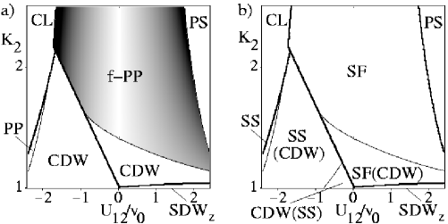
Figure 5: a) Phase diagram of a BFM, b) phase diagram of a BBM with the first species being in the hardcore limit, in terms of $U_{12}$, and the Luttinger parameter of the second species ($K_{2}$), at the fixed velocity ratio $|v_{1}-v_{2}|/(v_{1}+v_{2})=0.5$. For large repulsive interaction the system undergoes phase separation (PS), for large attractive interaction the system collapses (CL). In the regime below the thick line the system opens a gap, i.e. if species 2 is close to the hardcore limit. However, for larger values of $K_{2}$, the gapless phase is restored. Close to the transition, the properties of the fermions, respectively hardcore bosons, are still affected by the RG flow, leading to CDW order for the fermions and to supersolid behavior for the bosons.

In order to determine the QLRO in the system we will determine the scaling exponents of various order parameters. The order parameter with the largest positive scaling exponent shows the dominant order, whereas other orders with positive exponent are subdominant.

We will now apply this procedure to the different types of mixtures. For a FFM we find that the system always develops a gap, with the exception of the repulsive SU(2) symmetric regime (cp. [10]). To determine the QLRO we introduce the following operators [47, 25]: $O_{SS}=\sum_{\sigma,\sigma^{\prime}}\tilde{\sigma}f_{R,\sigma}\delta_{\sigma,\sigma^{\prime}}f_{L,3-\sigma^{\prime}}$, $O_{TS}^{a}=\sum_{\sigma,\sigma^{\prime}}\tilde{\sigma}f_{R,\sigma}\sigma^{a}_{\sigma,\sigma^{\prime}}f_{L,3-\sigma^{\prime}}$, $O_{CDW}=\sum_{\sigma,\sigma^{\prime}}f_{R,\sigma}^{\dagger}\delta_{\sigma,\sigma^{\prime}}f_{L,\sigma^{\prime}}$, and $O_{SDW}^{a}=\sum_{\sigma,\sigma^{\prime}}\tilde{\sigma}f_{R,\sigma}^{\dagger}\sigma^{a}_{\sigma,\sigma^{\prime}}f_{L,\sigma^{\prime}}$, with $\sigma,\sigma^{\prime}=1,2$, $\tilde{\sigma}=3-2\sigma$, and $a=x,y,z$. In the gapless SU(2) symmetric regime, both CDW and SDW show QLRO, with both scaling exponents of the form $\alpha_{SDW/CDW}=1-K_{\rho}$ [47], which shows that these orders are algebraically degenerate. Within the gapped regime the scaling exponents of these operators are given by $\alpha_{SS,TS_{z}}=2-K_{\rho}^{-1}$ and $\alpha_{CDW,SDW_{z}}=2-K_{\rho}$. As discussed in [25], the sign of $g_{12}$ determines whether CDW or SDW_z, and SS or TS_z appears. In Fig. 4 a), we show the phase diagram based on these results. In addition to these phases we indicate the appearance of the Wentzel-Bardeen instability, shown as phase separation for repulsive interaction and collapse for attractive interaction.

We will now use the dual mapping to obtain the phase diagram of a FFM with complementary filling from Fig. 4 a). Under this mapping, the attractive and repulsive regimes are exchanged with the following replacements: $CDW{\rightarrow}SDW_{z}$, $SDW_{z}{\rightarrow}CDW$, $SS,TS_{z}{\rightarrow}SDW$, and $SDW{\rightarrow}SS$. Note that the gapless regime is now on the attractive side, with degenerate CDW and SS pairing.

For BBMs we proceed in the same way as for FFMs. We introduce the following set of order parameters: $O_{CDW}=b_{1}^{\dagger}b_{1}+b^{\dagger}_{2}b_{2}$, $O_{SS}=b_{1}b_{2}$, $O_{SDW_{z}}=b_{1}^{\dagger}b_{1}-b^{\dagger}_{2}b_{2}$, $O_{SDW_{x}}=b_{1}^{\dagger}b_{2}+b^{\dagger}_{2}b_{1}$, $O_{SDW_{y}}=-i(b_{1}^{\dagger}b_{2}-b^{\dagger}_{2}b_{1})$, and in addition the superfluid (SF) order parameters $b_{1}$ and $b_{2}$. In Fig. 4 a) we show the phase diagram of a mixture of a BBM of hardcore bosons, which is almost identical to the one of a FFM. The phase diagram of the mixture with complementary filling, as obtained from the dual mapping, is also of the same form as its fermionic equivalent, with the exception of the gapless regime, in which BBMs show supersolid behavior (coexistence of SF and CDW order), and with the replacement $TS_{z}{\rightarrow}SS$.

In Fig. 5 b), we show the phase diagram of a mixture of hardcore bosons (species 1) and bosons in the intermediate to hardcore regime (species 2). If species 2 is sufficiently far away from the hardcore limit, the system remains gapless. However, in the vicinity of the transition the scaling exponents of the liquids are affected by the RG flow. As indicated, the effective scaling exponent of the hardcore bosons is renormalized to a value that is smaller than 1, and therefore we find both SF and CDW order, i.e. supersolid behavior. The phase diagram of the dual mixture is of the following form: the attractive and the repulsive regime are exchanged, and in the gapped phase we again have the mapping: $CDW{\rightarrow}SDW_{z}$, $SDW_{z}{\rightarrow}CDW$, $SS{\rightarrow}SDW$, and $SDW{\rightarrow}SS$. The gapless regime is unaffected.

For a BFM we find that the order parameters $O_{CDW}$, $O_{SDW_{z}}$, $O_{f-PP}=f_{R}f_{L}e^{-2i\lambda\Phi_{b}}$ [65, 69], and $b$ can develop QLRO in the gapless regime. In the gapped regime, the order parameters $O_{PP}\equiv f_{R}bf_{L}b$ and $O_{PP^{\prime}}\equiv f_{R}b^{\dagger}f_{L}b^{\dagger}$, in addition to $O_{CDW}$, show QLRO. ($O_{PP/PP^{\prime}}$ are special cases of the polaron pairing operators discussed in [65, 69].) In Fig. 4 b) we show the phase diagram of a BFM with hardcore bosons, and in Fig. 5 a), we vary the Luttinger parameter of the bosons. In both the gapless phase and the gapped phase, we find that CDW and $f$-PP or PP, respectively, are mutually exclusive and cover the entire phase diagram, cp. [65, 69]. The dual mapping again maps attractive and repulsive regimes onto each other. Within the gapped phase we find the mapping $CDW{\rightarrow}SDW_{z}$, $SDW_{z}{\rightarrow}CDW$, and $PP{\rightarrow}PP^{\prime}$, the gapless regime is unaffected.

Before we conclude, we discuss how these predictions could be measured experimentally. CDW order will create additional peaks in TOF images, corresponding to a wavevector $Q=2k_{f}$. As demonstrated and pointed out in [32, 21, 3, 66], the noise in TOF images allows to identify the different regimes of both gapped and gapless phases. As discussed in [65, 69], a laser stirring experiment could determine the onset of CDW order for fermions, or the supersolid regime for bosons. RF spectroscopy [12] can be used to determine the presence and the size of an energy gap.

In conclusion, we have studied mixtures of ultra-cold atoms in 1D with commensurate filling. We used a Luttinger liquid description which enables us to study FFMs, BFMs, and BBMs in a single approach. We find that FFMs are generically gapped for both attractive and repulsive interactions, whereas for BFMs and BBMs the bosons need to be close to the hardcore limit. We find a rich structure of quasi-phases in the vicinity of these transitions, in particular a supersolid phase for BBMs, that occurs close to the hardcore limit. Experimental methods to detect the predictions were also discussed.

IV. Phase-locking transition of coupled low-dimensional superfluids

Most phase transitions that have been realized in ultra-cold atom systems are generic first or second order transitions. However, the paradigm of phase transitions in two dimensions at finite temperature is of a more intricate type, a Kosterlitz-Thouless transition, which is characterized by a change of the functional form of the correlation function of the order parameter, from algebraic decay to exponential decay. In an intriguing new development in studying low-dimensional strongly correlated systems, such a Kosterlitz-Thouless (KT) transition [11] was indeed realized and observed [33]. In this experiment the interference amplitude between two independent two-dimensional (2D) Bose systems was studied as a function of temperature. This analysis revealed the jump in the superfluid stiffness (see also Ref. [85]) and the emergence of unpaired isolated vortices as they crossed the phase transition.

The other focus of this section, the physics of ramping across a phase transition, is also triggered by a recent experiment: Sadler et. al. observed spontaneous generation of topological defects in the spinor condensate after a sudden quench (i.e. a rapid, non-adiabatic ramp) through a quantum phase transition [89]. A similar experiment in a double-layer system was reported in Ref. [90]. The topological defects are generated [49] at a density which is related to the rate at which the transition is crossed [113]. Later it was argued that the dependence of the number of such defects on the swipe rate across a quantum critical point can be used as a probe of the critical exponents characterizing the phase transition [86]. This Kibble-Zurek (KZ) mechanism was originally considered as an early universe scenario creating cosmic strings, which would serve as an ingredient for the formation of galaxies [50]. Cold atom systems appear to be a very suitable laboratory for performing such “cosmological experiments”, since these systems are highly tunable and well isolated from the environment. So far the experiments and the theoretical proposals addressed the KZ scenario across a quantum phase transition. The main reason is that it is generally hard to cool such systems sufficiently fast to observe non-equilibrium effects. In this work we provide an example of a particular system where this difficulty can be easily overcome by quenching the transition temperature $T_{c}$ instead of $T$. Thus the relevant ratio $T/T_{c}$ can be tuned with an arbitrary rate and the KZ mechanism can be observed. Specifically, we examine a system of two superfluids (SF): As we show below, by turning on tunneling between the two systems the transition temperature increases rapidly, and the system attempts to create long-range order (LRO). However, in this process, defects in the SF phase are created, which develop into long-lived vortex-anti-vortex pairs or in finite system unbalanced population between vortices and anti-vortices. We note that because the systems are isolated and there is no external heat bath, the temperature itself also changes due to the quench. However, the long-wavelength fluctuations relevant for the KT transition are only a small subset of all degrees of freedom, majority of which are only weakly affected by small inter-layer tunneling. So we believe that the change of the $T_{c}$ is the main effect of the quench.

In this section we consider two SFs coupled via tunneling and/or interactions. In the experiments the hopping or tunneling rate between two systems can be tuned to a high precision [82, 33, 92, 34]. Interactions between the atoms in different systems can either be realized in ensembles of polar molecules or by using mixtures of two hyperfine states, where the tunneling rate is controlled by an infrared light source [44], which induces spin-flipping between the hyperfine states. In this case the atoms in different states naturally interact with each other since they are not physically separated in space. The main results of our analysis are the phase diagrams of coupled SFs in Fig. 6 and Fig. 7, the behavior of $T_{c}$ and the energy gap shown in Fig. 16, as well as the proposal of realizing the KZ mechanism by switching on the tunneling between two SFs.

Figure 6: Phase diagrams of two 2D SFs, coupled through a term of the form ${\mathcal{S}}_{12}$, Eq. (22), in terms of $J_{int}/J$ and $T/T_{KT}$. For low temperatures we find antisymmetric quasi-order (AQ) and/or symmetric quasi-order (SQ), which either simultaneously undergo a KT transition due to single vortices (AQ/SQ to thermal Bose gas (TBG) phase), or individually due to correlated vortex pairs: symmetric (anti-symmetric) vortex pairs drive the AQ/SQ to AQ (SQ) transition.

2D superfluids

In this section we consider two 2D SFs, each characterized by a KT temperature $T_{KT}$. We write the bosonic operators $b_{1/2}$ in the two layers in a phase-density representation [11, 27], $b_{1/2}\sim\sqrt{\rho_{1/2}}\exp(i\phi_{1/2})$, where $\rho_{1/2}$ are the density operators of the two systems, and $\phi_{1/2}$ the phases. The low-momentum fluctuations of the phase fields are described by Gaussian contributions to the Hamiltonian $\mathcal{H}_{0}$. Because of the formal analogy between the quantum 1D and thermal 2D systems [25] we adopt the quantum terminology throughout the paper and refer to the ratio of the Hamiltonian and the temperature as the action. Then

$${\mathcal{S}}_{0}\equiv\frac{{\mathcal{H}}_{0}}{T}=\frac{J}{2T}\int d^{2}r[(\nabla\phi_{1})^{2}+(\nabla\phi_{2})^{2}]\,.$$ (18)

The energy scale $J$ here is related to $T_{KT}$ by $J=2T_{KT}/\pi$. Besides these long-wavelength fluctuations, the system also contains additional degrees of freedom, vortex-anti-vortex pairs [11]. The corresponding term in the action is expressed through the dual fields $\theta_{1,2}$ [27]:

$${\mathcal{S}}_{1} = \frac{2A_{1}}{T}\int\frac{d^{2}r}{(2\pi\alpha)^{2}}[\cos(2\theta_{1})+\cos(2\theta_{2})]\,,$$ (19)

where $\alpha$ is a short-distance cut-off of the size of the vortex core, and $A_{1}$ is proportional to the single-vortex fugacity: $A_{1}\sim J\exp(-J/T)$, where we assume both SFs to have the same effective parameters $J$ and $A_{1}$. Operators of the type $\exp(2i\theta)$ create kinks in the field $\phi$: $\exp(-2i\theta(x))\phi(x^{\prime})\exp(2i\theta(x))\sim\phi(x^{\prime})+2\pi\Theta(x-x^{\prime})$, $\Theta(x)$ being the step function, which corresponds to the effect of vortices in the original 2D problem (Ref. [25], p. 92).

In addition the two systems are coupled by a hopping term $\sim t_{\perp}b_{1}^{\dagger}b_{2}+h.c.$, which results in the following contribution to the action:

$${\mathcal{S}}_{\perp} = \frac{2J_{\perp}}{T}\int\frac{d^{2}r}{(2\pi\alpha)^{2}}\cos(\phi_{1}-\phi_{2}),$$ (20)

where the bare value of $J_{\perp}$ corresponds approximately to $t_{\perp}\rho_{0}$. In principle, the hopping term is modified by the vortex contributions, however, these corrections are always irrelevant under renormalization group (RG).

For most of the discussion in this paper we use the symmetric and anti-symmetric combinations of $\phi_{1/2}$ and $\theta_{1/2}$:

$$\phi_{s/a}=(\phi_{1}\pm\phi_{2})/\sqrt{2},\quad\theta_{s/a}=(\theta_{1}\pm\theta_{2})/\sqrt{2}\,.$$ (21)

Written in these fields, the term ${\mathcal{S}}_{0}$ in Eq. (18) is again a sum of Gaussian models, now in the fields $\phi_{s}$ and $\phi_{a}$, with the same energy scale $J$. However, we will consider a broader class of actions, in which the energy scales of the symmetric and anti-symmetric sector differ. We include the following term in the action:

$${\mathcal{S}}_{12} = \frac{J_{{\rm int}}}{T}\int d^{2}r\nabla\phi_{1}\nabla\phi_{2}$$ (22)

With this, the quadratic part of the action is given by:

$${\mathcal{S}}_{0}+{\mathcal{S}}_{12} = \frac{J_{s}}{2T}\int d^{2}r(\nabla\phi_{s})^{2}+\frac{J_{a}}{2T}\int d^{2}r(\nabla\phi_{a})^{2}\,,$$ (23)

where $J_{s}$ and $J_{a}$ are given by $J_{s/a}=J\pm J_{{\rm int}}$.

We now motivate the existence of such a term ${\mathcal{S}}_{12}$ in ultracold atom systems, by considering two BECs coupled by a short-range density-density interaction. Starting from a Hamiltonian of the form $H=\sum_{k}[\epsilon_{\mathbf{k}}b^{\dagger}_{\mathbf{k}}b_{\mathbf{k}}+(g/2V)\rho_{\mathbf{k}}^{\dagger}\rho_{\mathbf{k}}$], where $b_{\mathbf{k}}$ is the boson operator, $\epsilon_{\mathbf{k}}$ the free dispersion $\epsilon_{\mathbf{k}}={\mathbf{k}}^{2}/2m$, $g$ is the interaction strength of the contact interaction, $V$ the volume, and $\rho_{\mathbf{k}}$ is the density operator of momentum ${\mathbf{k}}$, given by $\rho_{\mathbf{k}}=\sum_{\mathbf{p}}b^{\dagger}_{\mathbf{p}}b_{\mathbf{p}+\mathbf{k}}$, we assume that the zero momentum mode is macroscopically occupied, and formally replace the operator $b_{0}$ by a number, $b_{0}\rightarrow\sqrt{N_{0}}$, where $N_{0}$ is the number of condensed atoms which is comparable to the total atom number $N$, i.e. $N_{0}\sim N$. Next we keep all terms that are quadratic in $b_{\mathbb{k}}$ (with $\mathbb{k}\neq 0$), and perform a Bogoliubov transformation, given by: $b_{\mathbb{k}}=u_{\mathbb{k}}\beta_{\mathbb{k}}+v_{\mathbb{k}}\beta^{\dagger}_{\mathbb{-k}},$ to diagonalize the Hamiltonian. The eigenmodes $\beta_{\mathbb{k}}$ have a dispersion relation $\omega_{\mathbf{k}}=\sqrt{\epsilon_{\mathbf{k}}(\epsilon_{\mathbf{k}}+2gn)}$, with $n$ being the density $N/V$. The low-${\bf k}$ limit is given by $\omega_{\mathbb{k}}^{2}\sim v^{2}|{\bf k}|^{2}$, with $v=\sqrt{gn/m}$, which corresponds to the contribution in Eq. (18) of the action. Next, we consider the sum of two copies of the previous Hamiltonian with boson operators $b_{1/2}$. In addition we consider an interaction $H_{12}=g_{12}/V\sum_{\mathbf{k}}\rho_{1,\mathbf{k}}^{\dagger}\rho_{2,\mathbf{k}}$, where the density operators $\rho_{1/2,{\mathbf{k}}}$ are given by $\rho_{1/2,\mathbf{k}}=\sum_{\mathbf{p}}b^{\dagger}_{1/2,\mathbf{p}}b_{1/2,\mathbf{p}+\mathbf{k}}$. Following the same procedure as before, we find two eigenmode branches, corresponding to in-phase and out-of-phase superpositions of the modes of each condensate, with the dispersions $\omega_{s/a,\mathbb{k}}^{2}\sim v_{s/a}^{2}|{\bf k}|^{2}$, with the velocities $v_{s/a}=\sqrt{(g\pm g_{12})n/m}$. Therefore, for this example, the energy scale $J_{int}$ is related to $g_{12}n/m$, which would be of similar order as $J$ for a system interacting via contact interaction, for small temperatures. This discussion only applies to the weakly interacting limit of a true condensate. However, it demonstrate that a density-density contact interaction term can lead to a substantial energy splitting of the in-phase and out-of phase modes.

Figure 7: Phase diagram, temperature (in units of $T_{KT}$) versus interaction (in units of $J$). We assume $J_{\perp}/J\sim 10^{-3}$ and $A_{1}/J\sim 10^{-3}$. DLSF: double layer superfluid; TBG: thermal Bose gas; ASF: anti-symmetric superfluid; SQ: symmetric quasi-order. The order of the transition lines are either first (I), second order (II), or KT (thin lines).

Finally, in addition to single vortices in each SF, we have to consider the possibility of correlated vortex pairs, i.e. one vortex in each layer at the same location of either the same or of opposite vorticity. We will refer to these vortex configurations as symmetric or anti-symmetric vortex pairs, respectively. These excitations appear as the following terms in the action:

$${\mathcal{S}}_{s,a} = \frac{2A_{s,a}}{T}\int\frac{d^{2}r}{(2\pi\alpha)^{2}}\cos(2\sqrt{2}\,\theta_{s,a}).$$ (24)

These correlated vortex terms, which describe new degrees of freedom, can be the most relevant non-linear terms in the action, which derives from the possibility that the vortices in different layers interact with each other, through the terms (20) and (22). The effect of these terms is the following: At low temperatures the energy between two single vortices of opposite vorticity due to tunneling grows as the square of the distance D between them, i.e. as $J_{\perp}(D/\alpha)^{2}$. As a result, the tunneling term attempts to confine vortices of opposite vorticity, leading to phase-locking between the layers, which we describe further later on. The interaction ${\mathcal{S}}_{12}$ changes the energy of correlated vortex pairs as follows: The energy of a single vortex is given by $2\pi J\log L/\alpha$, where $L$ is the system size, whereas a symmetric/anti-symmetric vortex pair has an energy of $4\pi(J\pm J_{int})\log L/\alpha$. Therefore, symmetric vortex pairs are the lowest energy vortex excitations for $J_{int}<-J/2$, whereas for $J_{int}>J/2$ anti-symmetric vortex pairs are the lowest energy excitations. As we will see below, in these regimes correlated vortex pairs drive transitions to phases, in which one sector is (quasi-)SF whereas the other is disordered. We will also see that these terms are generated under the RG flow, even if not present at the onset.

We note that a similar system has been studied in [8]. Here, we consider a larger class of systems by including the interaction term (22), which in turn requires us to include the correlated vortex excitations (24). These terms give rise to additional phases as we will see in the following.

Next we analyze our system within the RG approach. This RG flow is perturbative in the vortex fugacities $A_{1}$, $A_{s}$, and $A_{a}$, and the tunneling energy $J_{\perp}$, and therefore applies to the weak-coupling limit (in particular $J_{\perp}\rightarrow+0$). At second order the flow equations are given by [6]:

$$\frac{dJ_{\perp}}{dl}=\left(2-\frac{T}{2\pi J_{a}}\right)J_{\perp}\,,$$ (25)

$$\frac{dA_{s}}{dl}=\left(2-2\pi\frac{J_{s}}{T}\right)A_{s}+\alpha_{3}\frac{A_{1}^{2}(J_{a}-J_{s})}{2T^{2}}\,,$$ (26)

$$\frac{dA_{a}}{dl}=\left(2-2\pi\frac{J_{a}}{T}\right)A_{a}+\alpha_{3}\frac{A_{1}^{2}(J_{s}-J_{a})}{2T^{2}}\,,$$ (27)

$$\frac{dA_{1}}{dl}=\left(2-\frac{\pi(J_{s}+J_{a})}{2T}+\alpha_{3}\frac{A_{s}J_{s}+A_{a}J_{a}}{T^{2}}\right)A_{1}\,,$$ (28)

$$\frac{dJ_{a}}{dl}=\alpha_{2}\Big{(}\frac{J_{\perp}^{2}}{4\pi^{4}J_{a}}-4\frac{A_{a}^{2}}{T^{4}}J_{a}^{3}-\frac{A_{1}^{2}}{2T^{4}}(J_{s}+J_{a})J_{a}^{2}\Big{)},\phantom{XX}$$ (29)

$$\frac{dJ_{s}}{dl}=-\alpha_{2}\Big{(}2\frac{A_{s}^{2}}{T^{4}}J_{s}^{2}+\frac{A_{1}^{2}}{4T^{4}}(J_{s}+J_{a})J_{s}\Big{)}2J_{s}\,.$$ (30)

The coefficients $\alpha_{2/3}$ are non-universal parameters that appear in the RG procedure [56], and which do not affect the results qualitatively. For consistency, we have to expand the right-hand site of the above equations up to second order, around the resulting Gaussian fixed point: $J_{s/a}=J\pm J_{{\rm int}}+j_{s/a}$. We emphasize again that $J_{int}$ near the fixed point can be generated by RG and be nonzero even if it is not present at the onset.

Before we consider the full RG flow, we consider the simpler case of no tunneling, i.e. we solve the RG equations while setting $J_{\perp}=0$. In Fig. 6 we show the phase diagram of two 2D SFs coupled by ${\mathcal{S}}_{12}$, Eq. (22). Such a system would be realized by a 2D mixture of bosonic atoms in two different hyperfine states, interacting via some short-range potential. The order parameters we consider are $O_{s}(x)=b_{1}(x)b_{2}(x)$ and $O_{a}(x)=b_{1}^{\dagger}(x)b_{2}(x)$. To obtain the phase diagram we consider the correlation functions of each of these order parameters, which can either scale algebraically or exponentially. In Fig. 6 we refer to algebraic scaling of $O_{s}(x)$ as symmetric quasi-order (SQ), and of $O_{a}(x)$ as anti-symmetric quasi-order (AQ). In each of the sectors a KT transition marks the transition from the algebraic to the exponential regime, which occur either simultaneously and are driven by single-vortex excitations, or at different temperatures and are driven by correlated vortex pairs. As a result we find four regimes: At temperatures above $T_{KT}$, both sectors are disordered, giving rise to a thermal Bose gas (TBG) phase. For temperatures below $T_{KT}$, and for a wide range of $J_{int}$, we find that both sectors are quasi SF (AQ/SQ), which is the only phase in which the correlation function of the single boson operators show algebraic scaling. We also find regimes in which only one sector shows algebraic scaling, whereas the other is disordered (AQ and SQ). From the perspective of vortices, the TBG phase is a gas of free single vortices in each layer, whereas the AQ (SQ) phase is a gas of symmetric (anti-symmetric) vortex pairs.

We now consider the full RG system, including $J_{\perp}$. We numerically integrate the RG equations, and find the phase diagram shown in Fig. 7 in terms of the temperature $T$ and the interaction $J_{\rm int}$. We again find four different phases that are different combinations of LRO, QLRO, and disorder in the symmetric and anti-symmetric sector. At high temperatures we find that both sectors are disordered in a TBG phase, as before. For lower temperatures, and for a wide range of $J_{{\rm int}}$, the system is in a double-layer SF phase (DLSF): The symmetric sector shows algebraic scaling, whereas the exponent of the anti-symmetric sector is renormalized to zero, i.e. we find two SFs that are phase-locked due to $J_{\perp}$. Note that the transition temperature $T_{c}$ between DLSF and TBG has been noticeably increased relative to the decoupled value $T_{KT}$, as we will discuss further later on. We also find two additional phases, which are partially (quasi-)SF and partially disordered. One of them is the SQ phase, as before, whereas the other one (ASF), now shows true LRO in the anti-symmetric sector due to $J_{\perp}$, whereas the symmetric sector remains disordered. We note that the generic double-layer action that we discuss in this paper does not show a sliding phase [76], for any non-zero $J_{\perp}$. Either $S_{1}$ or $S_{a}$, which is generated by RG, drives the anti-symmetric sector to a disordered state, or $S_{\perp}$ creates true LRO in the field $\phi_{a}$.

We also use the RG flow to find the order of the phase transitions in the weak-coupling limit that the anti-symmetric sector undergoes, by determining the energy gap using a ’poor-man’s scaling’ argument: when the coupling amplitude $J_{\perp}(l^{*})$ is of order unity the corresponding gap is given by the expression $\Delta\sim J_{\perp}\exp(-l^{*})$. From the behavior of $\Delta$ at the phase transition we can read off whether it is of first or second order, as indicated in Fig. 7.

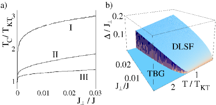
Figure 8: (a) Critical temperature $T_{c}$ of the DLSF-TBG transition (in units of $T_{KT}$) for different values of $A_{1}/J$: $10^{-3},0.1,0.4$ (I–III), and for $J_{\rm int}=0$. (b) Energy gap in the anti-symmetric sector (in units of $J_{\perp}$) as a function of $J_{\perp}/J$ and temperature (in units of $T_{KT}$). We have set $A_{1}/J=0.1$ and $J_{int}=0$.

Given the nature of an effective theory, only approximate statements can be made about how the different regimes of the phase diagram relate to the microscopic interactions. To create the ASF or AQ phase an attraction between the two atom species is needed that is of order $J$, whereas to create the SQ phase, a repulsion of that order would be needed. To detect the different phases, one could use the interference method used in [33] to distinguish the phase-locked phases (DLSF and ASF), which would show a well-defined interference pattern, from the uncorrelated phases. Another approach would be time-of-flight images: The DLSF phase would display a quasi-condensate signature, whereas the other phases would appear disordered. However, at the transition from ASF or SQ to TBG, the width of the distribution would abruptly increase.

Kibble-Zurek mechanism

In this section we discuss how the phase-locking transition found in the previous section could be used to realize the KZ mechanism. The defining property of this mechanism is the generation of topological defects by ramping across a phase transition, coming from the disordered phase. The disordered phase that we propose to use is the TBG phase of the decoupled 2D systems, that is, we consider the experimental setup reported in ref. [33] for a temperature $T$ above the KT temperature $T_{KT}$. The ordered phase we consider is the DLSF phase, i.e. the phase-locked phase of two coupled SFs. The ramping is achieved by turning on the tunneling between the two layers, which can be done by lowering the potential barrier between them. For this procedure the critical temperature $T_{c}$ of the DLSF-TBG transition needs to be above the KT temperature of the uncoupled systems. We now show that the RG flow indeed predicts such a scenario. In the experiments in Ref. [33], the atoms in different layers do not interact with each other. Therefore, it can be expected that $J_{\rm int}$ is small, of order $J_{\perp}$, which motivates us to discuss the case $J_{int}=0$ here. We note however, that the desired scenario of an increased critical temperature, is found for a wide range of $J_{int}$, as can be seen in Fig. 7. In Fig. 16 (a) we show how the critical temperature of the DLSF-TBG transition behaves, predicted by the RG flow, for different values of $A_{1}$. The critical temperature shows a sizeable increase, due to the phase-locking transition. Due to the perturbative nature of the RG scheme, the RG flow underestimates the effects of the term $S_{1}$, and predicts a finite jump of the critical temperature when $J_{\perp}$ is turned on. However, to lock the SFs together in the regime slightly above $T_{KT}$, $J_{\perp}$ needs to be at least of the order of the vortex core energy, giving rise to a finite slope of $T_{c}$ instead of a jump. The energy gap of this transition is shown in Fig. 16 from which we can see that the transition is of first order, in contrast to the second order transition described in [49, 113], which is advantageous because the onset of order is instantaneous rather than continuous. We note that the phase diagram was obtained using the assumption that the bare parameters of the model, in particular $J$, do not depend on temperature. This is true only if temperature is close to $T_{KT}$. Here we find that the ratio $T_{c}/T_{KT}$ can be relatively large. In fact $T_{c}/T_{KT}$ will be always smaller than that shown in Fig 16 (a), however, qualitatively the behavior of $T_{c}/T_{KT}$ as a function of $J_{\perp}$ should remain intact. We point out that our results can be generalized to a system of $N>2$ coupled SFs. One finds that the SFs still show a strong tendency to phase-lock together. As a result the critical temperature should approximately satisfy the equality $\pi J(T_{c})N=2T_{c}$. Thus as $N$ increases $T_{c}$ approaches the mean-field critical temperature at which the stiffness $J$ vanishes and we recover the usual 3D result.

In finite size systems there is another constraint on the minimum value of $J_{\perp}$: We consider the free energy of a single vortex in the anti-symmetric field: $\phi_{a}\sim\arctan(x/y)$. For the decoupled system we get for the free energy [56]: $F\sim 2(\pi J-2T)\log L/\alpha$, where $L$ is the system size. The coupling term gives a free energy contribution $F_{\perp}\sim J_{\perp}(L/\alpha)^{2}$. In the thermodynamic limit, $L\rightarrow\infty$, this term diverges faster than the others, which is consistent with our finding of LRO in the antisymmetric sector. For a finite system, comparing these terms gives the estimate $J_{\perp}\sim J\log(L/\alpha)/(L/\alpha)^{2}$, that is required for this order to develop. With a system size $L/\alpha\sim 10^{2}$, that would require $J_{\perp}\sim 10^{-3}J$, which, for the setup in [33], would be around $10^{2}s^{-1}$.

As an estimate of the number of domains that would be created, we follow the argument in [49]: The coherence scale of the DLSF phase is given by $(J/\Delta)^{1/2}\alpha$, which is the scale of a Klein-Gordon model with a kinetic energy scale $J$ and a ’mass-term’ with a prefactor $\Delta/\alpha^{2}$. The domain size is then given by $(J/\Delta)\alpha^{2}$, and the number of domains by $\sim(\Delta/J)L^{2}/\alpha^{2}$. As we show in Fig. 16 b) for $J_{\perp}/J\approx 10^{-2}$, we find $\Delta/J_{\perp}\sim 10^{-1}$, and therefore $J/\Delta\sim 10^{3}$. With $L/\alpha\sim 10^{2}$, we would get $N_{dom}\sim 10^{1}-10^{2}$, which would generate a similar number of vortices. We estimate the vortex-antivortex imbalance by considering the number of domains around the periphery of the system, which scales as $L/\xi$. If we imagine that the phase behaves like a random walk, the total phase mismatch, corresponding to the vortex-antivortex imbalance, will scale as $\sqrt{L/\xi}\sim N_{dom}^{1/4}$, which, for $L/\alpha\sim 10^{2}$, is of the order $10^{0}-10^{1}$.

In summary, we propose the following procedure: i) Prepare two uncoupled SFs at a temperature $T$ slightly above $T_{KT}$. ii) Switch on the tunneling between the two layers, which creates a DLSF phase with a critical temperature $T_{c}$ higher than $T$. As a result, one should find a number of long-lived vortex-antivortex pairs in the anti-symmetric phase field $\phi_{a}$, which would be visible in an interference measurement, at a temperature where there would be none in thermal equilibrium.

In conclusion of the section, we studied the phase-locking transition of 2D superfluids, within an renormalization group approach. We find that this transition is accompanied by an increase of the transition temperature. We suggest that this effect can be used to probe the Kibble-Zurek mechanism in cold atom systems by rapidly changing the ratio $T/T_{c}$. When we include interactions between the layers we find additional phases, in which either the symmetric or the anti-symmetric sector is disordered, and the other sector stays superfluid or quasi-superfluid.

V. Bose-Fermi mixtures in two-dimensional optical lattices

In the spirit of engineering many-body systems that are relevant in other fields, we now turn to atomic mixtures that resemble qualitatively, i.e. in terms of degrees of freedom of the system, electron-phonon systems. In two dimensions, these systems are actively studied and prove to be of considerable complexity. In order to study their atomic counterparts, Bose-Fermi mixtures in optical lattices, we use the powerful method of functional renormalization group equations, with which we can determine their phase diagrams in the weak-coupling limit in a systematic fashion. We find a rich competition of phases for both the square lattice and triangular lattice geometry that we consider.

In this section we consider mixtures of one bosonic type of atom and either two fermionic types that are SU(2) symmetric or spinless fermions. The Hamiltonian for a mixture on a square lattice is given by:

$$H\!=\!-t_{f}\sum_{\langle ij\rangle,s}f^{\dagger}_{i,s}f_{j,s}\!-\!t_{b}\sum_{\langle ij\rangle}b^{\dagger}_{i}b_{j}\!-\!\sum_{i}(\mu_{f}n_{f,i}\!+\!\mu_{b}n_{b,i})\!+\!\sum_{i}\Big{[}U_{ff}n_{f,i,\uparrow}n_{f,i,\downarrow}\!+\!\frac{U_{bb}}{2}n_{b,i}n_{b,i}\!+\!U_{bf}n_{b,i}n_{f,i}\Big{]}\,,$$ (31)

where $f^{\dagger}_{i,s}$ ($f_{i,s}$) creates (annihilates) a fermion at site $i$ with pseudo-spin $s$ ($s=\uparrow,\downarrow$), $b^{\dagger}_{i}$ ($b_{i}$) creates (annihilates) a boson at site $i$, $n_{f,i}=\sum_{s}f^{\dagger}_{i,s}f_{i,s}$ ($n_{b,i}=b^{\dagger}_{i}b_{i}$) is the fermion (boson) number operator, $t_{f}$ and $t_{b}$ are the fermionic and bosonic tunneling energies between neighboring sites, $\mu_{f}$ ($\mu_{b}$) is the chemical potential for fermions (bosons), $U_{bb}$ is the repulsion energy between bosons on the same site, $U_{ff}$ is the repulsion energy between the two species of fermions, and $U_{bf}$ is the repulsion energy between bosons and fermions. The two fermion species have been treated as a pseudo-spin-$1/2$ index ($\uparrow$ and $\downarrow$). The case of spinless fermions can be immediately obtained from (31) by ignoring one of the spin states. In momentum space, the Hamiltonian (31) is written as:

$$H\!=\!\sum_{\mathbf{k}}\left\{\!(\epsilon_{f,\mathbf{k}}\!-\!\mu_{f})\sum_{s}f^{\dagger}_{\mathbf{k},s}f_{\mathbf{k},s}\!+\!(\epsilon_{b,\mathbf{k}}\!-\!\mu_{b})b^{\dagger}_{\mathbf{k}}b_{\mathbf{k}}\!+\!\frac{U_{ff}}{V}\rho_{f,\mathbf{k},\uparrow}\rho_{f,-\mathbf{k},\downarrow}\!+\!\frac{U_{bb}}{2V}\rho_{b,\mathbf{k}}\rho_{b,-\mathbf{k}}\!+\!\frac{U_{bf}}{V}\rho_{b,\mathbf{k}}\rho_{f,-\mathbf{k}}\!\right\}\,,$$ (32)

where $\rho_{f,{\bf k}}=\sum_{{\bf q},s}f^{\dagger}_{\mathbf{k}+{\bf q},s}f_{\mathbf{k},s}$ ($\rho_{b,{\bf k}}=\sum_{{\bf q}}b^{\dagger}_{\mathbf{k}+{\bf q}}b_{\mathbf{k}}$) is the fermion (boson) density operator, $\epsilon_{b/f,\mathbf{k}}=-2t_{b/f}(\cos k_{x}+\cos k_{y})$, is the bosonic/fermionic dispersion relation.

We consider the limit of weakly interacting bosons that form a BEC [109, 67], where we assume that the zero momentum bosonic mode is macroscopically occupied, and the corresponding operator $b_{0}$ can be formally replaced by a real number $b_{0}\rightarrow\sqrt{N_{0}}$, where $N_{0}$ is the number of condensed atoms. After this replacement we keep all terms that are quadratic in $b_{\mathbf{k}}$ (with $\mathbf{k}\neq 0$), and perform a Bogoliubov transformation, given by: $b_{\mathbf{k}}=u_{\mathbf{k}}\beta_{\mathbf{k}}+v_{\mathbf{k}}\beta^{\dagger}_{\mathbf{-k}},$ to diagonalize the bosonic Hamiltonian. The resulting eigenmodes $\beta_{\mathbf{k}}$ have a dispersion relation given by $\omega_{\mathbf{k}}=\sqrt{\epsilon_{b,\mathbf{k}}(\epsilon_{b,\mathbf{k}}+2U_{bb}n_{b})}$ , with the low-${\bf k}$ limit $\omega_{\mathbf{k}}\sim v_{b}|{\bf k}|$, with $v_{b}=\sqrt{2t_{b}U_{bb}n_{b}}$. The parameters $u_{\mathbf{k}}$ and $v_{\mathbf{k}}$ are given by: $u_{\mathbf{k}}^{2}=(\omega_{\mathbf{k}}+\epsilon_{b,\mathbf{k}}+U_{bb}n_{b})/(2\omega_{\mathbf{k}})$ and $v_{\mathbf{k}}^{2}=(-\omega_{\mathbf{k}}+\epsilon_{b,\mathbf{k}}+U_{bb}n_{b})/(2\omega_{\mathbf{k}})$.

The density fluctuations of the bosons are approximated by: $\rho_{b,\mathbf{k}}\approx\sqrt{N_{0}}(u_{\mathbf{k}}+v_{\mathbf{k}})(\beta_{\mathbf{k}}+\beta_{-\mathbf{k}}^{\dagger})$, with $\mathbf{k}\neq 0$. The interaction between bosons and fermions is then given by $U_{bf}\sqrt{N_{0}}/V\sum_{\mathbf{k}}(u_{\mathbf{k}}+v_{\mathbf{k}})(\beta_{\mathbf{k}}+\beta_{-\mathbf{k}}^{\dagger})\rho_{f,-\mathbf{k}}$. As a next step we integrate out the bosonic modes and use an instantaneous approximation, leading to the following effective Hamiltonian:

$$H_{{\rm eff.}}=\sum_{\mathbf{k}}\left\{(\epsilon_{\mathbf{k}}-\mu_{f})\sum_{s}f^{\dagger}_{\mathbf{k},s}f_{\mathbf{k},s}+\frac{U_{ff}}{V}\rho_{f,\mathbf{k},\uparrow}\rho_{f,-\mathbf{k},\downarrow}+\frac{1}{2V}V_{{\rm ind.},\mathbf{k}}\,\,\rho_{f,\mathbf{k},}\rho_{f,\mathbf{-k}}\right\}\,,$$ (33)

where the induced potential $V_{{\rm ind.},\mathbf{k}}$ is given by:

$$V_{{\rm ind.},\mathbf{k}}=-\tilde{V}/(1+\xi^{2}(4-2\cos k_{x}-2\cos k_{y}))\,,$$ (34)

with $\tilde{V}$ given by $\tilde{V}=U_{bf}^{2}/U_{bb}$, and $\xi$ is the healing length of the BEC and is given by $\xi=\sqrt{t_{b}/2n_{b}U_{bb}}$. This approach is only valid when $v_{b}\gg v_{f}$, so that the fermion-fermion interaction mediated by the bosons can be considered as instantaneous. Away from this limit, retardation effects are present. In this case, one has to consider the frequency dependence of the interaction explicitly [55, 102, 103]. The full effective interaction, including retardation, is given by:

$$V_{\rm ind.}(\omega,\mathbf{k})=-\left[\frac{\tilde{V}}{1+\xi^{2}(4-2\cos{k_{x}}-2\cos{k_{y}})}\right]\frac{\omega^{2}_{\mathbf{k}}}{\omega^{2}+\omega^{2}_{\mathbf{k}}},$$ (35)

and the static limit (34) is recovered when $\omega_{\mathbf{k}}\gg\omega$. Equation (33) describes the scattering of two fermions from momenta ${\bf k}_{1}$ and ${\bf k}_{2}$, that are scattered into momenta ${\bf k}_{3}$ and ${\bf k}_{4}$. Momentum conservation at the interaction vertex requires that ${\bf k}_{4}={\bf k}_{1}+{\bf k}_{2}-{\bf k}_{3}$, and hence the interaction vertex, $U(\mathbf{k}_{1},\mathbf{k}_{2},\mathbf{k}_{3})$, depends on three momenta. Its bare value from (33) can be written as:

$$U(\mathbf{k}_{1},\mathbf{k}_{2},\mathbf{k}_{3}) = U_{ff}+V_{{\rm ind.},\mathbf{k}_{1}-\mathbf{k}_{3}}\,.$$ (36)

For the case with retardation, there is dependence on both the momenta and frequencies of the electrons so we have $U(k_{1},k_{2},k_{3})$, with $k_{4}=k_{1}+k_{2}-k_{3}$, where $k_{i}=(\omega,{\mathbf{k}})$.

Starting from non-interacting fermions, we ask the general question of what new many-body phases can emerge when the system is subjected to a given interaction $U(\mathbf{k}_{1},\mathbf{k}_{2},\mathbf{k}_{3})$. Our approach to address this question is the renormalization-group method, described in the next section.

Renormalization-Group Method

Starting with a microscopic model of interacting electrons on a lattice, the renormalization-group (RG) method provides the effective model at a given temperature or energy scale [94]. The RG is implemented by systematically tracing out high energy degrees of freedom in a region between $\Lambda$ and $\Lambda+d\Lambda$, where $\Lambda$ is the energy cut-off of the problem. In this process, the vertex $U$ is renormalized. At the initial value of the cut-off $\Lambda=\Lambda_{0}$, the value of $U$ is given by its bare value. For the BFM system we describe here it is given by (36). At one loop, the RG flow is obtained from a series of coupled integral-differential equations [111] for all the different interaction vertices $U(\mathbf{k}_{1},\mathbf{k}_{2},\mathbf{k}_{3})$. The RG equations read:

$$\partial_{\ell}U_{\ell}(\!{\bf k_{1}},\!{\bf k_{2}},\!{\bf k_{3}}\!)\!=\!-\!\!\!\int_{p,\omega}\!\!\partial_{\ell}[G_{p\ell}G_{k\ell}]U_{\ell}(\!{\bf k_{1}},\!{\bf k_{2}},\!{\bf k}\!)U_{\ell}(\!{\bf p},\!{\bf k},\!{\bf k_{3}}\!)\!-\!\!\int_{p,\omega}\!\!\partial_{\ell}[G_{p\ell}G_{q_{1}\ell}]U_{\ell}(\!{\bf p},\!{\bf k_{2}},\!{\bf q_{1}}\!)U_{\ell}(\!{\bf k_{1}},\!{\bf q_{1}},\!{\bf k_{3}}\!)$$

$$\!\!-\!\!\!\int_{p,\omega}\!\!\!\!\partial_{\ell}[G_{p\ell}G_{q_{2}\ell}]\!\!\left\{-\!2U_{\ell}(\!{\bf k_{1}},\!{\bf p},\!{\bf q_{2}}\!)U_{\ell}(\!{\bf q_{2}},\!{\bf k_{2}},\!{\bf k_{3}}\!)\!+\!U_{\ell}(\!{\bf p},\!{\bf k_{1}},\!{\bf q_{2}}\!)U_{\ell}(\!{\bf q_{2}},\!{\bf k_{2}},\!{\bf k_{3}}\!)\!+\!U_{\ell}(\!{\bf k_{1}},\!{\bf p},\!{\bf q_{2}}\!)U_{\ell}(\!{\bf k_{2}},\!{\bf q_{2}},\!{\bf k_{3}}\!)\!\right\}$$ (37)

where $\ell=\ln(\Lambda_{0}/\Lambda)$, ${\bf k}={\bf k}_{1}+{\bf k}_{2}-{\bf p}$, ${\bf q}_{1}={\bf p}+{\bf k}_{2}-{\bf k}_{3}$, ${\bf q_{2}}={\bf p}+{\bf k}_{1}-{\bf k}_{3}$, and $G_{k\ell}=\Theta(|\xi_{{\bf k}}|-\Lambda)/(i\omega-\xi_{{\bf k}})$ with $\xi_{\bf k}=\epsilon_{f,{\bf k}}-\mu_{f}$ and $k=(\omega,\bf k)$.

From the general interaction vertices $U(\mathbf{k}_{1},\mathbf{k}_{2},\mathbf{k}_{3})$, the specific interaction channels, such as charge-density wave (CDW), antiferromagnetic (AF), and superconducting (BCS), can be obtained:

$$V^{CDW} = 4\,\,U_{c}(\mathbf{k}_{1},\mathbf{k}_{2},\mathbf{k}_{1}+\mathbf{Q})\,,$$ (38)

$$V^{AF} = 4\,\,U_{\sigma}(\mathbf{k}_{1},\mathbf{k}_{2},\mathbf{k}_{1}+\mathbf{Q})\,,$$ (39)

$$V^{BCS} = U(\mathbf{k}_{1},-\mathbf{k}_{1},\mathbf{k}_{2})\,,$$ (40)

where we have used the notation: $U_{c}=(2-\hat{X})U/4$, $U_{\sigma}=-\hat{X}U/4$ with $\hat{X}U(\mathbf{k}_{1},\mathbf{k}_{2},\mathbf{k}_{3})=U(\mathbf{k}_{2},\mathbf{k}_{1},\mathbf{k}_{3})$, and $\mathbf{Q}$ is the nesting vector, $\mathbf{Q}=(\pi,\pi)$.

In a numerical implementation, one discretizes the Fermi surface into $M$ patches, and hence each of the interaction channels (38), (39), (40) is represented by an $M\times M$ matrix. At each RG step, we diagonalize each of these matrices. The channel with the largest eigenvalue (with the caveat that a BCS-channel needs to be attractive to drive a transition) corresponds to the dominant order. The elements of the eigenvector are labeled by the discrete patch indices around the Fermi surface and the symmetry of the order parameter is given by this angular dependence.

The RG method for interacting fermions has been extended to also include retardation effects, as for the case of interacting electrons which are also coupled to phonons in a crystal [102, 103]. In this case: (i) the interaction vertices also depend on frequencies of the incoming and outgoing fermions, so the RG equations are written for given external frequencies and the integral over intermediate frequencies can not be done analytically, and (ii) there are important self-energy corrections (in particular the imaginary part of the self-energy is non-zero). Eliashberg equations for strong-coupling superconductivity has been derived with this method [102, 103] for the case of electrons, with a circular Fermi surface, coupled to phonons. This method has also been applied to other electron-phonon problems [99, 54], and to mixtures of cold atoms in an optical lattice [55].

Phase Diagram and Sub-Dominant Orders

The microscopic parameters in the Hamiltonian (31) determine the initial conditions for the RG flow, and the shape of the Fermi surface. With these, we write the RG flow equations and solve them numerically. We first discuss the case without retardation. For some parameters, we encounter a divergence in the RG flow, indicating the onset of ordering with a gap that is in the detectable regime, i.e. larger than $10^{-3}t_{f}$. In other regimes, where such a divergence is not reached, one can read off the dominant tendency of the RG flow. In Fig. 9 we show examples of RG flows as a function of $\ell$. In Fig. 9 (a), we show the competition between d-wave and s-wave pairing, with d-wave being dominant and s-wave being subdominant. In Fig. 9 (b) we show an example with dominant d-wave channel and subdominant AF channel. In both cases we find that for short distances (or high energies) CDW fluctuations are dominant, giving rise to a state that resembles the findings for high-$T_{c}$ superconductors [37, 36, 105]. In some situations the many-body states are almost degenerate and small changes in the initial conditions (that is, changes in the form of the interactions) can be used to select one particular ground state.

With this procedure we determine the phase diagram of the system, which is shown in Fig. 10. We now discuss the general features of the phase diagram. In the absence of any coupling to the bosons, i.e. for $\tilde{V}=0$, the system shows s-wave pairing for attractive interaction, $U_{ff}<0$, and no ordering for $U_{ff}>0$, i.e. Fermi liquid behavior, except for the special case of half-filling where Fermi surface nesting drives the system to AF order for repulsive interactions, and to s-wave pairing (degenerate with CDW) for attractive interaction. If we now turn on the interaction to the bosons, this picture is modified in the following way: The boundary of the s-wave regime is moved into the regime of positive $U_{ff}$, approximately to a value of $U_{ff}$ where the effective interaction at the nesting vector ${\bf Q}$ between the fermions, $U_{ff}+V_{{\rm ind.},\mathbf{Q}}$, is positive, i.e. for $U_{ff}\approx\tilde{V}/(1+8\xi^{2})$. On the repulsive side, and away from half-filling, we find the tendency to form a paired state, either $d$-wave or $p$-wave. This tendency becomes weaker the further the system is away from half-filling. We typically find a gap in the vicinity of half-filling and further away from $\mu=0$ we find only an increasing strength of the corresponding interaction channel. For the half-filled system, we find that for attractive interactions the degeneracy between $s$-wave pairing and CDW ordering is lifted, with $s$-wave pairing being the remaining type of order. For repulsive interactions, we find an intermediate regime of $d$-wave pairing, and for larger values of $U_{ff}$ we obtain AF order.

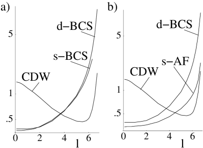
Figure 9: RG flow for the different effective interactions (in units of $t_{f}$) as a function of the RG parameter $l$ ($\tilde{V}/t_{f}=3$ and $\xi=1$). a) $U_{ff}/t_{F}=0.5$; b) $U_{ff}/t_{f}=1.2$.

Figure 10: Phase diagram, interaction strength, $U_{ff}/t_{f}$, versus number of fermions per site, $n$, for a Fermi-Bose mixture in a square lattice in 2D ($\tilde{V}/t_{f}=2$, $\xi=1$).

The RG approach also allows the extraction of the many-body gaps in the system through a ”poor man’s scaling” analysis of the divergent flow: at the point where the coupling becomes of order of $t_{f}$ the scaling parameter $\ell$ reaches the maximum value $\ell_{c}=\ln(t_{f}/\Delta)$, where $\Delta$ is the value of the gap. Hence, $\Delta/t_{f}\approx\exp\{-\ell_{c}\}$ can be obtained from the RG flows such as the ones in Fig. 9. In Fig. 11 we show the gaps of the problem as a function of $U_{ff}/t_{f}$ in the half-filled case. One can see that as $U_{ff}$ increases, from negative to positive values, the $s$-wave gap is replaced by a $d$-wave gap, and finally for an antiferromagnetic gap. As is apparent from this figure, the gap in the $d$-wave phase is much smaller than the gaps of the AF order and the $s$-wave pairing, and, furthermore, almost independent of the value of $U_{ff}$. The latter is the case because the $U_{ff}$ term is a pure $s$-wave contribution to the interaction and therefore does not contribute to the $d$-wave channel. The $d$-wave channel has an initial contribution which is entirely due to the anisotropy of the induced interaction, which gives only a small value, and as a consequence only a small value for the gap. The value of the gap (in units of $t_{f}$) can be numerically fitted with a BCS expression of the form $a\exp(-b/\tilde{V})$, with the parameters $a$ and $b$ given by $a=0.31$ and $b=14.2$.

Figure 11: Many-body energy gaps at half-filling ($\mu=0$), as a function of $U_{ff}/t_{f}$, for $\tilde{V}/t_{f}=3$ and at a fixed value of the coherence length $\xi=1$. Dashed line: s-wave gap; Continuous line: d-wave gap; Dotted-dashed line: antiferromagnetic gap. The inset shows a magnified plot of the d-wave regime.

For a system of spinless fermions, one can simply suppress one of the spin indices in (31) and (32). In this case there is a major simplification in the problem since $U_{ff}$ is absent: in a spinless problem there can be only one fermion per site, as per Pauli’s principle. Hence, in the absence of bosons, the spinless gas is non-interacting. The bosons, however, mediate the interaction between the fermions. Since the fermions are in different lattice sites the pair wavefunction has necessarily a node and hence, no $s$-wave pairing is allowed. In other words, in the spinless case the anti-symmetry of the wavefunction requires pairing in an odd angular momentum channel. In fact, we find that throughout the entire phase diagram the fermions develop $p$-wave pairing. At half-filling we find a similar behavior of CDW fluctuations on short scales, analogous to the flow shown in Fig. 9. One should point out that in real solids the conditions of ”spinlessness” behavior is hard to achieve since it usually requires complete polarization of the electron gas, that is, magnetic energies of the order of the Fermi energy (a situation experimentally difficult to achieve in good metals). However, in cold atom lattices this situation can be easily accomplished with the correct choice of atoms.

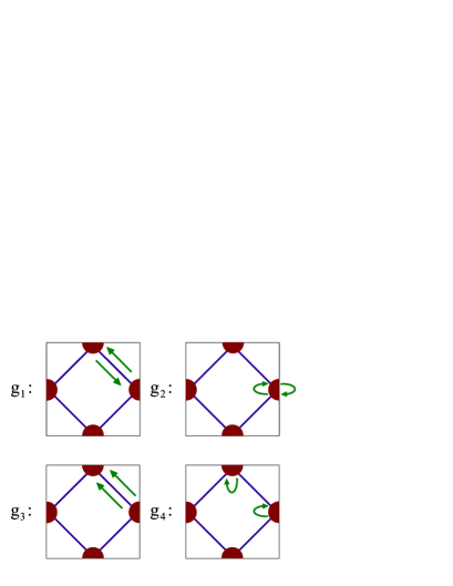
Figure 12: Relevant processes in the two-patch approximation.

Finally, when retardation is important, the numerical task of solving the RG flow equations become much more demanding. In addition to the discretization of the Fermi surface, one has to also discretize the frequency (for $T=0$), or consider a certain number of Matsubara frequencies ($T\neq 0$). This has been done for this Bose-Fermi system only for a fixed density of fermions corresponding to one half [55]. In this case the Fermi surface has a diamond shape and scattering processes are dominated by the van Hove points (corners of the diamond) where the density of states is singular. The Fermi surface can therefore be approximated by the van Hove points only [91] so that he types of relevant processes are reduced, as shown in Fig. 12. Each of the processes still depend on frequencies: $g_{i}(\omega_{1},\omega_{2},\omega_{3})$, for $i=1,2,3,4$. The phase diagram is shown in Fig. 13. Retardation leads to additional phases at half-filling and by tuning the lattice parameters, the system undergoes AF (or spin-density-wave SDW), $d$-wave SC pairing, $s$-wave-pairing, and CDW. In the limit of $v_{b}\gg v_{f}$ discussed previously, when retardation is not important, CDW does not become dominant (Fig. 10). It is at most degenerate with $s$-wave pairing for $U_{ff}<0$. As the bosons become slower, there is stronger tendency for CDW formation (Fig. 13).

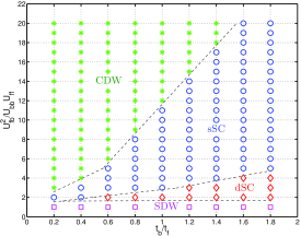
Figure 13: (Color online) Phase diagram for $U_{ff}=0.4t_{f}$, $U_{bb}=0.8t_{f}$, and $n_{b}=2.5$. Blue circles indicate $s$-wave SC, red rhombuses indicate $d$-wave SC, magenta squares AF (also called spin-density-wave SDW), and green stars CDW type of ordering. Dashed lines are guides to the eye.

Quantum Frustration in Triangular Lattices

It is known that the geometric shape of the lattice is a crucial factor in determining the properties of interacting many-body systems. For instance, localized spins interacting antiferromagnetically on a triangular lattice suffer from the phenomenon of frustration, when antiferromagnetic order cannot be achieved because of the particular lattice structure. For itinerant fermionic systems, the lattice structure, together with the dispersion relation and the filling fraction, determine the shape of the Fermi surface. The Fermi surface, by its turn, is a crucial factor in determining what type of orders the system can develop. Indeed, for the triangular lattice we consider in this Section, which shows a rich and subtle competition between superconducting phases with different symmetries, small changes in the shape of the FS determine which pairing symmetry is dominant. This is a reflection of the “lattice frustration” on the superconducting phases. In solids, this intriguing lattice geometry is realized in materials such as cobaltates [98], transition metal dichalcogenides [110] and $\kappa$-(ET)₂X layered organic crystals [43] (if each lattice site is represented by one ET dimer [51]), and has been the subject of several theoretical studies [101, 38, 108, 5, 59, 13, 23, 112]

In this section we consider a BFM on a triangular lattice. The geometry of the lattice under consideration here is shown in Fig. 15(a). This system is described by a similar Hubbard model as for the square lattice. But now, besides the triangular geometry, we allow for two different values for the hopping amplitudes, for two types of lattice bonds, as indicated in Fig. 15 a) by dashed and continuous lines. $t_{f,a}$ and $t_{b,a}$ with $a=1,2$ are the fermionic and bosonic tunneling amplitudes between neighboring sites, where the index $a=1$ ($a=2$) refers to the continuous (dashed) bonds. For the description of the isotropic case we equate $t_{b/f,1}$ and $t_{b/f,2}$, and define $t_{f}\equiv t_{f,1}=t_{f,2}$ and $t_{b}\equiv t_{b,1}=t_{b,2}$. $\mu_{f}$ ($\mu_{b}$) is the chemical potential for fermions (bosons), $U_{bb}$, $U_{ff}$, and $U_{bf}$ are the on-site boson-boson, fermion-fermion and boson-fermion repulsion energy, respectively.

Just as for the case of a square lattice (Sec. VII), we consider the limit of weakly interacting bosons, in which the bosons form a BEC, for which we use the same description. The resulting dispersion relation is now given by $\omega_{\mathbf{k}}=\sqrt{(\epsilon_{b,\mathbf{k}}-\epsilon_{b,0})(\epsilon_{b,\mathbf{k}}-\epsilon_{b,0}+2U_{bb}n_{b})}$, where the bare lattice dispersion is given by:

$$\epsilon_{b,k}=-t_{b,1}2\cos k_{x}-t_{b,2}(2\cos(k_{x}/2+\sqrt{3}k_{y}/2)+2\cos(k_{x}/2-\sqrt{3}k_{y}/2)).$$ (41)

For small values of $k_{x}$ and $k_{y}$, $\omega_{\mathbf{k}}$ can be expanded as: $\omega_{\mathbf{k}}\sim\sqrt{((2t_{b,1}+t_{b,2})k_{x}^{2}+3t_{b,2}k_{y}^{2})U_{bb}n_{b}}$, which gives us the two velocities $v_{b,x}=\sqrt{(2t_{b,1}+t_{b,2})U_{bb}n_{b}}$ and $v_{b,y}=\sqrt{3t_{b,2}U_{bb}n_{b}}$.

We again assume that these velocities of the condensate fluctuations are much larger than the Fermi velocity, which corresponds to the conditions $v_{b,x/y}>t_{f,1/2}$. Therefore, large bosonic hopping amplitudes, a bosonic density of $\approx 1$–$3$, and some intermediate value for $t_{f,1/2}$ will satisfy this requirement. As before, the bosonic modes can be integrated out, and we obtain an approximately non-retarded fermion-fermion interaction. The induced potential $V_{{\rm ind.},\mathbf{k}}$ is given by: $V_{{\rm ind.},\mathbf{k}}=-\tilde{V}/(1+\xi_{1}^{2}(2-2\cos k_{x})+\xi_{2}^{2}(4-4\cos(k_{x}/2)\cos(\sqrt{3}k_{y}/2)))$ with $\tilde{V}=U_{bf}^{2}/U_{bb}$, and $\xi_{a}$ are the healing lengths of the Bose-Einstein condensate (BEC) and are given by $\xi_{a}=\sqrt{t_{b,a}/2n_{b}U_{bb}}$ with $a=1,2$. We again arrive at a purely fermionic, non-retarded description of the same form as before. This is the effective model that we study with a numerical implementation of the functional renormalization group.

Figure 14: a) Fermi surfaces for an isotropic lattice, for $\mu_{f}<2t_{f,1/2}$, $\mu_{f}=2t_{f,1/2}$ (hexagonal shape), and $\mu_{f}>2t_{f,1/2}$ (six disjoint arcs). b) Diagram of the different types of Fermi surfaces that can be created on an anisotropic lattice, by varying the ratio $t_{f,2}/t_{f,1}$ and $\mu_{f}$. c) Fermi surfaces for $t_{f,2}<t_{f,1}$, for $\mu_{f}<4t_{f,2}-2t_{f,1}$, $4t_{f,2}-2t_{f,1}<\mu_{f}<2t_{f,1}$, and $\mu_{f}>2t_{f,1}$, corresponding to the regimes I–III, respectively. d) Fermi surfaces for $t_{f,2}>t_{f,1}$, for $\mu_{f}<2t_{f,1}$, $2t_{f,1}<\mu_{f}<4t_{f,2}-2t_{f,1}$, and $\mu_{f}>4t_{f,2}-2t_{f,1}$, corresponding to the regimes IV–VI, respectively.

For the isotropic case, perfect nesting occurs at 3/4-filling, with three possible nesting vectors: $\mathbf{Q}_{1}=(0,2\pi)$, $\mathbf{Q}_{2}=(\pi,\sqrt{3}\pi)$, and $\mathbf{Q}_{3}=(-\pi,\sqrt{3}\pi)$, leading to three different possible types of instabilities per density wave channel. For the anisotropic case, only $\mathbf{Q}_{1}$ can be a nesting vector, for the condition $\mu_{f}=2t_{f,1}$. To determine the scale of the gaps, $\Delta$, associated with each of these order parameters, we again use a ’poor man’s’ scaling estimate, specifically: $\Delta\approx\Lambda_{0}e^{-\ell_{c}}$, where $\ell_{c}$ is the point at which the RG flow diverges and the instability occurs.

The RG is implemented numerically by discretizing the FS into $M$ patches. For the results shown in this Section, $M=24$ or $36$ was used. The CDW, AF and BCS channels are diagonalized at each RG step. The dominant instability is the channel that has an eigenvalue (divided by the dimension of the matrix) with the largest magnitude (for BCS one has to ensure that such eigenvalue is negative so that the channel is attractive). Each element of the corresponding eigenvector represents a given FS patch, and hence, the symmetry of the dominant order parameter is reflected on the patch (i.e., angular) dependence of each element around the FS. Using this method, we determine the phase diagram of the system in various limits.

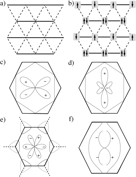
Figure 15: a) Lattice geometry of the system. The continuous (dashed) bonds correspond to the hopping amplitudes $t_{b/f,1(2)}$. For $t_{b/f,1}=t_{b/f,2}$, the lattice is an isotropic triangular lattice. b) schematic representation of the AF order corresponding to nesting vector ${\bf Q}_{1}$. c) + d) Order parameters of the extended $d$-wave orders $D_{1}$ and $D_{2}$. e) Order parameter of the $f$-wave phase. This order can also be interpreted as two $s$-wave paired hole states whose order parameters are out of phase by $\pi$. f) Order parameter of the extended $p$-wave phase, that appears in anisotropic lattices.

We first consider spin-$1/2$ fermions on an isotropic triangular lattice, i.e. with $t_{f,1}=t_{f,2}\equiv t_{f}$. The FS for such a lattice behaves as follows: For small filling the FS consists of one near-circular piece, which then approaches the shape of a hexagon as $\mu_{f}$ approaches the special value $\mu_{f}=2t_{f}$. At this special chemical potential, which corresponds to $3/4$-filling, the FS is nested with the three distinct nesting vectors ${\mathbf{Q}}_{i}$. For filling fractions larger than $3/4$ the FS breaks into six disjoined arcs. Examples for these different regimes are shown in Fig. 14 a). Without coupling to the BEC, the fermions form an $s$-wave pairing phase for attractive interactions, and a Fermi liquid phase for repulsive interactions (ignoring high angular momentum pairing phases predicted by the Kohn-Luttinger theorem [58] which would occur at energy scales much lower than the experimentally accessible regime), except for the specific case $\mu_{f}=2t_{f}$, where the system shows AF order for repulsive interactions. A schematic picture of this order is shown in Fig. 15 b) for the nesting vector $\mathbf{Q}_{1}$. This behavior is similar to the one found for isotropic square lattice in the previous Section [67]: $s$-wave pairing for attractive interaction, and Fermi liquid behavior for repulsive interaction, except at an special filling, for which we find AF order due to nesting. An interesting difference for the triangular lattice is the three-fold degeneracy of the AF phase, an indication of frustration.

When the coupling to the BEC is turned on, the isotropic triangular lattice shows a phase diagram of the type shown in Fig. 16. The $s$-wave pairing phase slightly extends into the regime of positive $U_{ff}$, because of the induced attractive interaction mediated by the bosonic fluctuations. The regime that showed Fermi liquid behavior in the absence of the induced interaction now shows a rich competition of various types of pairing. In the regime where the density is below half-filling, when the FS is approximately circular, the system shows $p$-wave pairing. For fillings larger than $3/4$, when the FS consists of six disjoined parts, the fermions Cooper pair in a superconducting state with $f$ symmetry. As shown in Fig. 15 e), the FS in this regime can also be interpreted as two distinct near-circular Fermi surfaces of holes. In this interpretation each of these two fermionic systems is in an $s$-wave pairing phase, but the relative phase between the two order parameters is $\pi$. At $3/4$-filling and large values of $U_{ff}$, the system still shows AF order. However, for smaller values of $U_{ff}$, and also for smaller fillings, two phases with degenerate extended $d$ symmetry develop. These superconducting orders have a sizeable $g$-wave component and are approximately given by:

$$\psi_{D_{1}} = \sin 2\theta+0.5\sin 4\theta$$ (42)

$$\psi_{D_{2}} = \cos 2\theta-0.5\cos 4\theta$$ (43)

These order parameters are shown in Fig. 15 c) and d). The shapes of the order parameters are energetically advantageous because, on the one hand, the order parameter maxima are located at points at which the system has a high density of states (the ’corners’ of the FS). Hence, when the superconducting gap opens, there is a large gain of condensation energy coming from these regions on the FS. On the other hand, the $d$-wave state has lower kinetic energy than the $f$-wave, and hence is selected.

The phase diagram Fig. 16 has a number of similarities to the phase diagram for a BFM on a square lattice, such as the $s$- and the $p$-wave pairing phase, and the existence of AF order for a nested Fermi surface for large $U_{ff}$.

Figure 16: Phase diagram of a Bose-Fermi mixture on a 2D isotropic triangular lattice. The vertical axis corresponds to the interaction strength, $U_{ff}/t_{f}$, whereas the horizontal axis corresponds to the filling fraction of the fermions per site, $n$. The other parameters are given by $\tilde{V}/t_{f}=3$, and $\xi_{a}=1$ with $a=1,2$.

However, the competition of pairing orders for positive $U_{ff}$ and intermediate and large filling is much richer, due to the more complex shape of the Fermi surface.

The energy gaps associated with these order parameters can be determined as we did in the previous Section [67], by using a ’poor man’s’ scaling argument. We find for the $s$-wave pairing and the AF order, that they are around $0.1T_{F}$, where $T_{F}$ is the Fermi temperature of the system. For most of the exotic phases, we energy gaps of the order of $0.01-0.001T_{F}$.

We now consider a BFM with spin-$1/2$ fermions on an anisotropic triangular lattice, i.e. with unequal hopping amplitudes, $t_{f(b),1}\neq t_{f(b),2}$. The shape of the FS behaves as follows: For $t_{f,2}>t_{f,1}$, as one increases the chemical potential, the FS first breaks into four arcs at $\mu_{f}=2t_{f,1}$, and then breaks into six arcs at $\mu_{f}=4t_{f,2}-2t_{f,1}$, corresponding to the regimes IV–VI, in Fig. 14 b) and d). For $t_{f,2}<t_{f,1}$ the FS first breaks into two arcs at $\mu_{f}=4t_{f,2}-2t_{f,1}$, and then breaks into six arcs at $\mu_{f}=2t_{f,1}$ coresponding to the regimes I–III, in Fig. 14 b) and c). At the special chemical potential $\mu_{f}=2t_{f,1}$ the FS is still nested, but there is only one nesting vector along the direction of the bonds with hopping amplitude $t_{f,1}$. In the absence of the coupling to the BEC the phase diagram has a similar structure as for the isotropic case: $s$-wave pairing for attractive interaction, Fermi liquid behavior for repulsive interaction, with the exception of the nested FS at $\mu_{f}=2t_{f,1}$ where one finds AF order (notice that in this case the filling is not $3/4$).

When the coupling to the bosons is turned on, one generates an even more complicated competition of pairing phases for repulsive $U_{ff}$ in the vicinity of the point $\mu_{f}=2t_{f,1}$, as is shown in Fig. 17. Generally, for unequal hopping the degeneracy between $D_{1}$ and $D_{2}$ in (43), as well as $p_{x}$ and $p_{y}$ is lifted: In the regime with $t_{f,2}>t_{f,1}$ ($t_{f,2}<t_{f,1}$), $D_{1}$ ($D_{2}$) and $p_{x}$ ($p_{y}$) dominate. For $t_{f,2}>t_{f,1}$, in the intermediate regime, in which the FS consists of four disjoined arcs, corresponding to the regime V in Fig. 14, the type of ordering changes from $D_{1}$ to $f$. For $t_{f,2}<t_{f,1}$, the type of pairing also eventually becomes $f$-wave, but first develops two other types of pairing, in the regime II in Fig. 14. Firstly, one finds an unusual extended $p$-wave symmetry, which is schematically shown in Fig. 15 f). Its wavefunction is of the form:

$$\psi_{P_{ext}} = \left\{\begin{array}[]{cr}\sin^{2}\theta&-\pi/2<\theta<\pi/2\\ -\sin^{2}\theta&\pi/2<\theta<3\pi/2\end{array}\right.$$ (46)

The second type of pairing that appears before the system develops $f$-wave pairing is $D_{1}$. These unusual pairing states are energetically favorable because of the anisotropic shape of the FS. For the regime in which the FS has just barely broken up into two arcs, the order parameter assumes $p$-wave symmetry and the maxima are located along the $y$-axis, where the density of states is highest. As the region of open FS widens (see Fig. 15 f)), this pairing becomes energetically unfavorable, and the system develops $D_{1}$-pairing, so that the maxima of the order parameter can again be located near the point of highest density of states. The energy gaps associated with these order parameters are of the same order of magnitude as for the isotropic lattice.

Figure 17: Phase diagram of a Bose-Fermi mixture on an anisotropic triangular lattice. The vertical axis corresponds to the ratio $t_{f,2}/t_{f,1}$, the horizontal axis corresponds to the chemical potential $\mu_{f}$. The other parameters are given by $\tilde{V}/t_{f}=3$, $U_{ff}/t_{f,1}=2$, and $\xi_{a}=1$ with $a=1,2$).

Finally, we consider a BFM with spinless fermions on an isotropic lattice. Due to the absence of $s$-wave scattering between fermions of the same spin state, there is no direct interaction, that is, $U_{ff}=0$. Hence, in the absence of bosons, the spinless gas is non-interacting. The boson fluctuations, however, mediate an induced interaction between the fermions. Due to the anti-symmetry of the Cooper pair wavefunction, pairing occurs in an odd angular momentum channel. We find a competition between $p$ and $f$-wave pairing symmetry. For small to intermediate filling ($n<0.65$), $p$-wave pairing dominates. For larger fillings, for which the FS first approaches the shape of a hexagon and then breaks up into six arcs, the system shows $f$-wave pairing. Since these larger fillings of fermions are typically realized in the center of an atomic trap, this result would suggest a comparatively easy way to create an exotic pairing state experimentally. In contrast to this, a spinless BFM on a square lattice only shows $p$-wave pairing, since for the quadrangular shape of its FS, channels of higher angular momentum are of no advantage energetically.

The many-body states discussed in this section can be observed through various methods: AF order could be revealed in time-of-flight images and Bragg scattering [96], noise correlations [32, 21, 3, 66] can be used to detect the various pairing phases, laser stirring experiments [87, 77] can be used to detect the phase boundary between AF order and pairing. The short-scale CDW fluctuations should give a signature in a photo-association measurement. RF spectroscopy [12] can be used to quantify the gaps of the various phases.

VI. Conclusions

In this article we studied the phase diagrams of various low-dimensional ultracold atom systems. In Section III we studied atomic mixtures in one dimension, using Luttinger liquid theory. We argued that a Bose-Fermi mixture can be naturally looked at as a Luttinger liquid of polarons, and we discussed the rich phase diagrams of commensurate mixtures. In Section IV, we studied the phases of two coupled two-dimensional superfluids at finite temperature. We found that that the critical temperature of the phase-locked phase is significantly increased over its bare value, which we propose to use for realizing the Kibble-Zurek mechanism. When interactions between the two superfluids are present, we find additional phases which are partially superfluid, and partially disordered. In Section V, we used the powerful method of functional renormalization group equations to determine the phases of Bose-Fermi mixtures in two-dimensional optical lattices. We found an intricate competition of orders, including new types of exotic pairing for triangular lattices. In all these sections, ideas how to probe our predictions were also given.

VII. Bibliography

Primary Literature:

Books and Reviews

Leggett AJ (2001) Bose-Einstein condensation in the alkali gases: Some fundamental concepts. Rev Mod Phys 73:307

Bloch I, Dalibard J, Zwerger W (2007) Many-Body Physics with Ultracold Gases. Rev. Mod. Phys. (to appear), arXiv:0704.3011v1

References

- [1] A.P. Albus, et al., Phys. Rev. A 67, 063606 (2003).
- [2] A.S. Alexandrov and S.N. Mott, Polarons and Bipolarons (World Scientific, Singapore, 1995).
- [3] Altman E, Demler E, and Lukin M (2004) Probing many-body states of ultracold atoms via noise correlations. Phys Rev A 70:013603
- [4] M. H. Anderson, J. R. Ensher, M. R. Matthews, C. E. Wieman, and E. A. Cornell, Observation of Bose-Einstein condensation in a Dilute Atomic Vapor Below 200 Nanokelvin, Science 269, 198 (1995).
- [5] Baskaran G (2003) Electronic model for CoO2 layer based systems: chiral resonating valence bond metal and superconductivity. Phys. Rev. Lett. 91:097003
- [6] L. Benfatto, et al., cond-mat/0609287.
- [7] M.J. Bijlsma, et al., Phys. Rev. A 61, 053601 (2000).
- [8] M.A. Cazalilla, J. Phys. B 37, S1-S47 (2004).
- [9] M. A. Cazalilla and A. F. Ho, Phys. Rev. Lett. 91, 150403 (2003).
- [10] M. A. Cazalilla, A.F. Ho, and T. Giamarchi, Phys. Rev. Lett. 95, 226402 (2005).
- [11] P.M. Chaikin and T.C. Lubensky, Principles of condensed matter physics, (Cambridge Univesrity Press, Cambridge, 1995).
- [12] Chin C, Bartenstein M, Altmeyer A, Riendl S, Jochim S, Hecker Denschlag J, and Grimm R (2004) Observation of the Pairing Gap in a Strongly Interacting Fermi Gas. Science 305:1128
- [13] Choy TP, Galanakis D, and Phillips P (2007) Proposed insulating ground state of Na0.5CoO2: Squaring the triangle. Phys. Rev. B 75:073103
- [14] K. B. Davis, M.-O. Mewes, M. R. Andrews, N. J. van Druten, D. S. Durfee, D. M. Kurn, and W. Ketterle, Bose-Einstein condensation in a gas of sodium atoms, Phys. Rev. Lett. 75, 3969 (1995).
- [15] Here we defined , , , , , and . is given by . These expressions are obtained from diagonalizing . Details will appear elsewhere.
- [16] de Pue MT, McCormick C, Winoto SL, Oliver S, and Weiss DS (1999) Unity occupation of sites in a 3D optical lattice. Phys Rev Lett 82:2262
- [17] S. Engelsberg and B.B. Varga , Phys. Rev. 136, A1582 (1964).
- [18] In this paper, we use to denote the optical lattice potential experienced by fermionic/bosonic atoms in the longitudinal (perpendicular) directions. Independent tuning of the optical lattices for two species of atoms can be achieved even with a single pair of lasers by controlling the laser detuning and intensity separately.
- [19] We note that in a homogeneous 1D system only quasi-long-range order for CDW phase is possible. However, the inhomogeneous trap boundary in a realistic experiment can pin the CDW phase to generate a true density modulation.
- [20] C. D. Fertig et al., cond-mat/0410491.
- [21] Fölling S, Gerbier F, Widera A, Mandel O, Gericke T, and Bloch I (2005) Spatial quantum noise interferometry in expanding ultracold atom clouds. Nature 434:481
- [22] J.N. Fuchs, A. Recati, and W. Zwerger, Phys. Rev. Lett. 93, 090408 (2004).
- [23] Gan JY, Chen Y, and Zhang FC (2006) Superconducting pairing symmetries in anisotropic triangular quantum antiferromagnets. Phys. Rev. B 74:094515
- [24] S.D. Gensemer and D.S. Jin, Phys. Rev. Lett. 87, 173201 (2001).
- [25] T. Giamarchi, Quantum Physics in one dimension, Clarendon Press (Oxford, UK, 2004).
- [26] A. Görlitz, et al. Phys. Rev. Lett. 87, 130402 (2001).
- [27] A.O. Gogolin, A.A. Nerseyan and A.M. Tsvelik, Bosonization and Strongly Correlated Systems (Cambridge University Press, 1998).
- [28] Goldwin J, Inouye S, Olsen ML, Newman B, DePaola BD, and Jin DS (2004) Measurement of the interaction strength in a Bose-Fermi mixture with Rb and K. Phys Rev A 70:021601
- [29] Greiner M, Bloch I, Mandel O, Hänsch TW, and Esslinger T (2001) Exploring phase coherence in a 2D lattice of Bose-Einstein condensates. Phys Rev Lett 87:160405
- [30] Greiner M, Mandel O, Esslinger T, Hänsch TW, and Bloch I (2002) Quantum phase transition from a superfluid to a Mott insulator in a gas of ultracold atoms. Nature 415:39
- [31] Greiner M, Regal CA, and Jin DS (2003) Emergence of a molecular Bose-Einstein condensate from a Fermi gas. Nature 426:537
- [32] Greiner M, Regal CA, Stewart JT, and Jin DS (2005) Probing Pair-Correlated Fermionic Atoms through Correlations in Atom Shot Noise. Phys. Rev. Lett. 94:110401
- [33] Z. Hadzibabic, P. Krüger, M. Cheneau, B. Battelier, J. B. Dalibard, Nature 441, 1118 (2006).
- [34] Z. Hadzibabic, S. Stock, B. Battelier, V. Bretin, and J. Dalibard, Phys. Rev. Lett. 93, 180403 (2004).
- [35] F. D. M. Haldane, Phys. Rev. Lett. 47, 1840 (1981).
- [36] Hanaguri T, Lupien C, Kohsaka Y, Lee D-H, Azuma M, Takano M, Takagi H, and Davis JC (2004) A ’checkerboard’ electronic crystal state in lightly hole-doped Ca2-xNaxCuO2Cl2. Nature 430:1001
- [37] Hoffman JE, Hudson EW, Lang KM, Madhavan V, Eisaki H, Uchida S, and Davis SC (2002) A four unit cell periodic pattern of quasi-particle states surrounding vortex cores in Bi2Sr2CaCu2O8+δ. Science 295:466
- [38] Honerkamp C (2003) Instabilities of interacting electrons on the triangular lattice. Phys. Rev. B 68:104510
- [39] Hubbard J (1963) Electron correlations in narrow energy band. Proc R Soc Lond A276:238
- [40] A. Isacsson and S. M. Girvin, Phys. Rev. A 72, 053604 (2005).
- [41] A. Isacsson, M.-C. Cha, K. Sengupta, and S. M. Girvin, Phys. Rev. B 72, 184507 (2005).
- [42] Jaksch D, Bruder C, Cirac JI, Gardiner CW, and Zoller P (1998) Cold bosonic atoms in optical lattices. Phys Rev Lett 81:3108
- [43] Jérome D (1991) The Physics of Organic Superconductors. Science 252:1509
- [44] G.-B. Jo, Y. Shin, S. Will, T. A. Pasquini, M. Saba, W. Ketterle, D. E. Pritchard, M. Vengalattore, M. Prentiss, cond-mat/0608585.
- [45] S. Jochim, M. Bartenstein, A. Altmeyer, G. Hendl, S. Riedl, C. Chin, J. H. Denschlag, R. Grimm, Science 302, 2101 (2003).
- [46] K. Jones, P. Julienne, P. Lett, W. D. Phillips, E. Tiesinga, and C. Williams, Measurement of the atomis Na(3P) lifetime and of retardation in the interaction between two atoms bound in a molecule, Europhys. Lett. 35, 85 (1996).
- [47] J. Voit, Rep. Prog. Phys., 58, 977 (1995).
- [48] C. Kane and M.P.A. Fisher, Phys. Rev. Lett. 68, 1220 (1992).
- [49] T. W. B Kibble, J. Phys. A 9, 1387 (1976).
- [50] Since then, it has been established that cosmic strings can only contribute a small fraction of the initial density perturbations. We thank T. Kibble for this comment.
- [51] Kino H and Fukuyama H (1995) Electronic states of conducting organic -(BEDT-TTF)2XJ. Phys. Soc. Jpn. 64:2726
- [52] T. Kinoshita, T. Wenger, and D. S. Weiss, Science 305, 1125 (2004).
- [53] A. Y. Kitaev, cond-mat/0010440
- [54] Klironomos FD and Tsai S-W (2006) Phonon-mediated tuning of instabilities in the Hubbard model at half-filling. Phys. Rev. B 74:205109
- [55] Klironomos FD and Tsai S-W (2007) Pairing and density-wave phases in Boson-Fermion mixtures at fixed filling. cond-mat/0702660
- [56] J. B. Kogut, Rev. Mod. Phys., 51, 659 (1979).
- [57] Köhl M, Moritz H, Stöferle T, Günter, and Esslinger T (2005) Fermionic atoms in a three dimensional optical lattice: observing Fermi surfaces, dynamics, and interactions. Phys Rev Lett 94:080403
- [58] Kohn W and Luttinger JM (1965) New Mechanism for Superconductivity. Phys. Rev. Lett. 15:524
- [59] S.-S. Lee and P. A. Lee (2005) Gauge Theory of the Hubbard Model: Spin Liquid States and Possible Application to -(BEDT-TTF)2Cu2(CN)3. Phys. Rev. Lett. 95:036403
- [60] P. D. Lett, P. S. Julienne, and W. D. Phillips, Photoassociative Spectroscopy of Laser-Cooled Atoms, Annu. Rev. Phys. Chem. 46, 423 (1995).
- [61] P. Maddaloni, et al., Phys. Rev. Lett. 85, 2413 (2000).
- [62] G.D. Mahan, Many-Particle Physics (Plenum Press, New York, 1990).
- [63] O. Mandel, M. Greiner, A. Widera, T. Rom, T. W. Hänsch, and I. Bloch, Phys. Rev. Lett. 91, 010407 (2003).
- [64] O. Mandel, M. Greiner, A. Widera, T. Rom, T. W. Hänsch, I. Bloch, Nature 425, 937 (2003).
- [65] Mathey L, Wang D-W, Hofstetter W, Lukin MD, Demler E (2004) Luttinger liquid of polarons in one-dimensional boson-fermion mixtures. Phys Rev Lett 93:120404
- [66] Mathey L, Altman E, Vishwanath A (2005) Noise Correlations in one-dimensional systems of ultra-cold fermions. Phys. Rev. Lett. 100, 240401 (2008).
- [67] Mathey L, Tsai S-W, and Castro Neto AH (2006) Competing types of order in two-dimensional Bose-Fermi mixtures. Phys Rev Lett 97:030601
- [68] Mathey L (2007) Commensurate mixtures of ultra-cold atoms in one dimension. Phys Rev B 75:144510
- [69] Mathey L, Wang D-W (2007) Phase diagrams of one-dimensional Bose-Fermi mixtures of ultra-cold atoms. Phys Rev A 75:013612
- [70] Mathey L, Tsai S-W, and Castro Neto AH (2007) Exotic superconducting phases of ultracold atom mixtures on triangular lattices. Phys Rev B 75:144510
- [71] Mathey L, Polkovnikov A, Castro Neto, AH (2008) Phase-locking transition of coupled low-dimensional superfluids. EuroPhys. Lett. 81, 10008.
- [72] Mckenzie RH (1997) Similarities Between Organic and Cuprate Superconductors. Science 278:820
- [73] Modugno G, Roati G, Riboli F, Ferlaino F, Brech RJ, and Inguscio M (2002) Collapse of a Degenerate Fermi Gas. Science 297:2240
- [74] Modugno G, Ferlaino F, Heidemann R, Roati G, and Inguscio M (2003) Production of a Fermi gas of atoms in an optical lattice. Phys Rev A 68:011601
- [75] H. Moritz, T. Stöferle, K. Günter, M. Köhl, and T. Esslinger, Phys. Rev. Lett. 94, 210401 (2005).
- [76] R. Mukhopadhyay, C. L. Kane, and T. C. Lubensky, Phys. Rev. B 64, 045120 (2001); C. S. O’Hern, T. C. Lubensky, and J. Toner, Phys. Rev. Lett. 83, 2745 (1999).
- [77] Onofrio R, Raman C, Vogels JM, Abo-Shaeer JR, Chikkatur AP, and Ketterle W (1999) Observation of Superfluid Flow in a Bose-Einstein Condensed Gas. Phys. Rev. Lett. 85:2228
- [78] Ospelkaus C, Ospelkaus S, Sengstock K, and Bongs K (2006) Interaction-driven dynamics of 40K-87Rb fermion-boson gas mixtures in the large-particle-number limit. Phys Rev Lett 96:020401
- [79] Ospelkaus C, Ospelkaus S, Humbert L, Ernst P, Sengstock K, and Bongs K (2006) Ultracold Heteronuclear Molecules in a 3D Optical Lattice. Phys Rev Lett 97:120402
- [80] Ospelkaus S, Ospelkaus C, Wille O, Succo M, Ernst P, Sengstock K, and Bongs K (2006) Localization of bosonic atoms by fermionic impurities in a three-dimensional optical lattice. Phys Rev Lett 96:180403
- [81] Ospelkaus S, Ospelkaus C, Humbert L, Sengstock K, and Bongs K (2006) Tuning of heteronuclear interactions in a degenerate Fermi-Bose mixture. Phys Rev Lett 97:120403
- [82] B. Paredes, A. Widera, V. Murg, O. Mandel, S. Foelling, I. Cirac, G. V. Shlyapnikov, T. W. Hänsch, and I. Bloch, Nature 429, 277 (2004).
- [83] G.B. Partridge, et al., cond-mat/0511752.
- [84] W. D. Phillips, C. Ekstrom, W. Goldin, and S. L. Rolston, Laser Cooling of Neutral Atoms for Frequency Standards, in Symposium on Frequency Standards and Metrology, ed. by J. Bergquist (World Scientific, Singapore, 1996), p. 5-10.
- [85] A. Polkovnikov, E. Altman, and E. Demler, Proc. Natl. Acad of Sci. USA 103, 6125 (2006).
- [86] A. Polkovnikov, Phys. Rev. B. 72, 161201(R) (2005); W. H. Zurek, U. Dorner, and P. Zoller, Phys. Rev. Lett. 95, 105701 (2005); J. Dziarmaga, Phys. Rev. Lett. 95, 245701 (2005).
- [87] Raman C, Köhl M, Onofrio R, Durfee DS, Kuklewicz CE, Hadzibabic Z, and Ketterle W (1999) Evidence for a Critical Velocity in a Bose-Einstein Condensed Gas. Phys. Rev. Lett. 83:2502
- [88] A. Recati, P. O. Fedichev, W. Zwerger, and P. Zoller, Phys. Rev. Lett. 90, 020401 (2003).
- [89] L. E. Sadler et al, Nature 443, 312 (2006).
- [90] D. R. Scherer et al, cond-mat/0610187.
- [91] Schulz HJ (1987) Superconductivity and antiferromagnetism in the two-dimensional Hubbard model – scaling theory. Europhys. Lett. 4:609
- [92] T. Schumm, S. Hofferberth, L. M. Andersson, S. Wildermuth, S. Groth, I. Bar-Joseph, J. Schmiedmayer, and P. Krüger, Nature Phys. 1, 57 (2005).
- [93] P. Sengupta and L. P. Pryadko, cond-mat/0512241.
- [94] Shankar R (1994) Renormalization group approach to interacting fermions. Rev Mod Phys 68:129
- [95] J. Solyom, Adv. Phys. 28, 201 (1979).
- [96] Stenger J, Inouye S, Chikkatur AP, Stamper-Kurn DM, Pritchard, and Ketterle W (1999) Bragg Spectroscopy of a Bose-Einstein Condensate. Phys. Rev. Lett. 82:4569
- [97] Stöferle T, Moritz H, Schori C, Köhl M, and Esslinger T (2004) Transition from a strongly interacting 1D superfluid to a Mott insulator. Phys Rev Lett 92:130403
- [98] Takada K, Sakurai H, Takayama-Muromachi E, Izumi F, Dilanian RA, and Sasaki T (2003) Nature 422:53
- [99] Tam K-M, Tsai S-W, Campbell DK, and Castro Neto AH (2007) Retardation effects in the Holstein-Hubbard chain at half filling. Phys. Rev. B 75:161103
- [100] Due to the confining trap the transition is, while visible, ’blurred’ into a gradual cross-over, due to finite size effects, and, more importantly, due to the coexistence of several phases in the trap. This can also be expected for the phase transitions predicted in this paper.
- [101] Tsai S-W and Marston JB (2001) -(BEDTTTF)2X organic crystals: Superconducting versus anti-ferromagnetic instabilities in the Hubbard model on an anisotropic triangular lattice. Can. J. Phys. 79:1463
- [102] Tsai S-W, Castro Neto AH, Shankar R, and Campbell DK (2005) Renormalization group approach to strong-coupled superconductors. Phys Rev B 72:054531
- [103] Tsai S-W, Castro Neto AH, Shankar R, and Campbell DK (2005) Renormalization group approach to superconductivity: from weak to strong electron-phonon coupling. Philos Mag 86:2631
- [104] S. Tsuchiya, A. Griffin, cond-mat/0311321.
- [105] Vershinin M, Misra S, Ono S, Abe Y, Ando Y, and Yazdani A (2004) Local ordering in the pseudogap state of the high- superconductor Bi2Sr2CaCu2O8+δ. Science 303:1995
- [106] L. Vichi et al., Phys. Rev. A 60, 4734 (1999).
- [107] J. Voit and H. J. Schulz, Phys. Rev. B 36, 968 (1987); ibid 37, 10068 (1988).
- [108] Vojta M and Dagotto E (1999) Indications of unconventional superconductivity in doped and undoped triangular antiferromagnets. Phys. Rev. B 59:713
- [109] Wang D-W, Lukin MD, and Demler E (2005) Engineering superfluidity in Bose-Fermi mixtures of ultracold atoms. Phys Rev A 72:(R)051604
- [110] Withers RL and Wilson JA (1986) An examination of the formation and characteristics of charge-density waves in inorganic materials with special reference to the two- and one-dimensional transition-metal chalcogenides. J. Phys. C 19: 4809
- [111] Zanchi D and Schulz HJ (2000) Weakly correlated electrons on a square lattice: Renormalization-group theory. Phys. Rev B 61:13609
- [112] Zhou A and Wang Z (2006) Charge and spin order on the triangular lattice – NaxCoO2 at . cond-mat/0608068
- [113] W. H. Zurek, Nature 317, 505 (1985).
- [114] M. W. Zwierlein, C. A. Stan, C. H. Schunck, S. M. F. Raupach, S. Gupta, Z. Hadzibabic, W. Ketterle, Phys. Rev. Lett. 91, 250401 (2003).
- [115] M. Zwierlein, et al., cond-mat/0511197.