Quantitative Rescattering Theory for high-order harmonic generation from molecules

Abstract

The Quantitative Rescattering Theory (QRS) for high-order harmonic generation (HHG) by intense laser pulses is presented. According to the QRS, HHG spectra can be expressed as a product of a returning electron wave packet and the photo-recombination differential cross section of the laser-free continuum electron back to the initial bound state. We show that the shape of the returning electron wave packet is determined mostly by the laser only. The returning electron wave packets can be obtained from the strong-field approximation or from the solution of the time-dependent Schrödinger equation (TDSE) for a reference atom. The validity of the QRS is carefully examined by checking against accurate results for both harmonic magnitude and phase from the solution of the TDSE for atomic targets within the single active electron approximation. Combining with accurate transition dipoles obtained from state-of-the-art molecular photoionization calculations, we further show that available experimental measurements for HHG from partially aligned molecules can be explained by the QRS. Our results show that quantitative description of the HHG from aligned molecules has become possible. Since infrared lasers of pulse durations of a few femtoseconds are easily available in the laboratory, they may be used for dynamic imaging of a transient molecule with femtosecond temporal resolutions.

I Introduction

High-order harmonic generation (HHG) has been studied extensively since 1990’s, both experimentally and theoretically. Initial interest in HHG was related to the generation of coherent soft X-ray beams krausz97 ; kapteyn97 , which are currently being used for many applications in ultrafast science experiments krausz09 ; thomann08 . In the past decade, HHG has also been used for the production of single attosecond pulses drescher ; sekikawa ; sansone and attosecond pulse trains apt , thus opening up new opportunities for attosecond time-resolved spectroscopy.

While HHG has been well studied for atoms, much less has been done for molecules. Initial interest in HHG from molecules was due to the fact that it offers promising prospects for increasing the low conversion efficiency for harmonic generation. The presence of the additional degrees of freedom such as the alignment and vibration opens possibilities of controlling the phase of the nonlinear polarization of the medium and of meeting the phase-matching condition. Thanks to the recent advancements in molecular alignment and orientation techniques seideman , investigation of the dependence of HHG on molecular alignment reveals the distinctive features of molecular HHG itatani05 as well as their structure itatani-nature . In particular, the existence of distinctive minima in the HHG spectra from H${}_{2}^{+}$ have been theoretically predicted by Lein et al. lein02 ; lein04 . The experimental measurements within the pump-probe scheme for CO₂ indeed showed the signature of these minima for partially aligned CO₂ kanai05 ; vozzi05 . More recently, newer experiments by JILA, Saclay, and Riken groups jila07 ; jila08 ; boutu ; riken08 began to focus on the phase of the harmonics, using mixed gases and interferometry techniques. These studies have revealed that near the harmonic yield minimum the phase undergoes a big change. In view of these experimental developments, a quantitative theory for HHG from molecular targets is timely.

HHG can be understood using the three-step model corkum ; kulander . First the electron is released into continuum by tunnel ionization; second, it is accelerated by the oscillating electric field of the laser and later driven back to the target ion; and third, the electron recombines with the ion to emit a high energy photon. A semiclassical formulation of this three-step model based on the strong field approximation (SFA) is given by Lewenstein et al lewenstein . In SFA, the liberated continuum electron experiences the full effect from the laser field, but not from the ion. In spite of this limitation, the model has been widely used for understanding the HHG by atoms and molecules. Since the continuum electron needs to come back to revisit the parent ion in order to emit radiation, the neglect of electron-ion interaction is clearly questionable. Thus, over the years efforts have been made to improve upon the SFA model, by including Coulomb distortion ivanov96 ; kaminski96 ; smirnova08 . These improvements, when applied to simple systems, however, still do not lead to satisfactory agreement with accurate calculations, based on numerical solution of the time-dependent Schrödinger equation (TDSE).

With moderate effort, direct numerical solution of the TDSE for atomic targets can be carried out, at least within the single active electron (SAE) approximation. For molecules, accurate numerical solution of the TDSE is much more computational demanding and has not been carried out except for the simplest molecules such as H${}_{2}^{+}$ lein02 ; kamta05 ; telnov07 . Thus most of the existing calculations for HHG from molecules were performed using the SFA model zhou05 ; zhou05b ; atle06 ; atle07 ; marangos06 ; seideman07 ; milosevic09 ; faisal09 . Additionally, in order to compare single molecule calculations with experimental measurements, macroscopic propagation of the emitted radiation field in a gas jet or chamber needs to be carried out, with input from calculations involving hundreds of laser intensities to account for intensity variation near the laser focus. For this purpose the TDSE method is clearly too time-consuming even for atomic targets.

In view of the inaccuracies of the SFA and the practical inefficiency of the TDSE method, we have proposed the quantitative rescattering theory or the QRS (also called the scattering-wave SFA or SW-SFA in our earlier papers atle08 ; H2+ ) as a simple and practical method for obtaining accurate HHG spectra. The main idea of the QRS is to employ exact transition dipoles with scattering wave instead of the commonly used plane-waves for the recombination step in a HHG process. Within the QRS, induced dipole moment by the laser can be represented as a product of the returning electron wave packet and the complex recombination transition dipole between free electrons with the atomic or molecular ion atle08 ; toru . The shape of the wave packet has been shown to be largely independent of the target. Therefore the returning wave packet can be calculated from the standard SFA model or by solving the TDSE from a reference atom with similar ionization potential as of the molecule under consideration. The QRS approach has been shown to be much more accurate than the standard SFA model for rare-gas atoms atle08 and a prototypical molecular system H${}_{2}^{+}$ H2+ . We note that the QRS has also been successfully used to explain high-energy electron spectra from various atomic systems chen-jpb09 ; chen09 ; sam-prl09 ; sam-jpb09 ; chen07 , and non-sequential double ionization sam-nsdi of atoms.

In order to use the QRS, we need to know the complex transition dipoles from aligned molecules. In other words, we need both the differential photoionization (or photo-recombination) cross section and the phase of the transition dipole for a fixed-in-space molecule. Calculations for these quantities can be carried out using the available molecular photoionization methods, which have been developed over the last few decades. In this paper we employ the iterative Schwinger variational method developed by Lucchese and collaborators lucchese82 ; lucchese95 .

The goal of this paper is to give a detailed description of all the ingredients of the QRS and demonstrate its validity. As examples of its application we consider HHG from aligned O₂ and CO₂ and show that the QRS is capable of explaining recent experiments. The rest of this paper is arranged as follows. In Sec. II we summarize all the theoretical tools needed for calculating HHG spectra from partially aligned molecules. We also explain how photoionization (photo-recombination) differential cross sections and phases of the transitions dipole are calculated for both atomic and molecular targets. The QRS model is formulated and its validity is carefully examined in Sec. III for atomic targets where results from the TDSE serve as “experimental” data. In Sec. IV we illustrate the application of the QRS method by considering the two examples of O₂ and CO₂ and compare the QRS results with available experiments. Sec. V discusses the predictions of the QRS for the minima in HHG spectra in relation to the simple two-center interference model. We also extend the QRS calculation for O₂ to higher photon energies by using 1600-nm lasers, to explore the interference effect in HHG spectra from O₂. Finally we finish our paper with a summary and outlook.

We note that the macroscopic propagation effect has not been treated in this paper jin09 . In the literature, theoretical treatments of such effects have been limited to atomic targets, and mostly starting with the SFA to calculate single atom response to the lasers. In this respect, the QRS offers an attractive alternative as the starting point since its calculation of single atom response is nearly as fast as the SFA, but with an accuracy much closer to the TDSE. Atomic units are used throughout this paper unless otherwise stated.

II Theoretical background

The theory part is separated into six subsections. We will describe all the ingredients used in the QRS. First we consider the TDSE and the SFA, as the methods to calculate HHG spectra and to extract returning electron wave packets. We will then present theoretical methods for calculation of photoionization (photo-recombination) cross sections for both atomic and linear molecular targets. We will also briefly describe intense laser ionization, as ionization rates are used in the QRS to account for depletion effect and overall normalization of the wave packets. Lastly, we explain how the partial alignment of molecules by an aligning laser is treated.

II.1 Method of solving the time-dependent Schrödinger equation

The method for solving the time-dependent Schrödinger equation (TDSE) for an atom in an intense laser pulse has been described in our previous works chen06 ; toru07 ; chen09 . Here we present only the essential steps of the calculations and the modifications needed to treat the HHG problem. At present accurate numerical solution of the TDSE for molecules is still a formidable computational task and has been carried out mostly for simple molecular systems such as H${}_{2}^{+}$ lein02 ; kamta05 ; telnov07 .

We treat the target atom in the single active electron model. The Hamiltonian for such an atom in the presence of a linearly polarized laser pulse can be written as

$$H=H_{0}+H_{i}(t)=-\frac{1}{2}\nabla^{2}+V(r)+H_{i}(t).$$ (1)

The atomic model potential $V(r)$ is parameterized in the form

$$V(r)=-\frac{1+a_{1}e^{-a_{2}r}+a_{3}re^{-a_{4}r}+a_{5}e^{-a_{6}r}}{r},$$ (2)

which can also be written as the sum of a short-range potential and an attractive Coulomb potential

$$V(r)=-\frac{1}{r}+V_{s}(r),$$ (3)

The parameters in Eq. (2) are obtained by fitting the calculated binding energies from this potential to the experimental binding energies of the ground state and the first few excited states of the target atom. The parameters for the targets used in this paper can be found in tong-jpb05 . One can also use a scaled hydrogen as a reference atom, as shown in Ref. atle08 ; H2+ . Here the effective nuclear charge is rescaled such that the ionization potential of the rescaled H(1s) matches the $I_{p}$ of the atom or molecule under consideration.

The electron-field interaction $H_{i}(t)$, in length gauge, is given by

$$H_{i}(t)={\bm{r}}\cdot{\bm{E}}(t).$$ (4)

For a linearly polarized laser pulse (along the $z$ axis) with carrier frequency $\omega$ and carrier-envelope-phase (CEP), $\varphi$, the electric field is taken to have the form

$${\bm{E}}(t)=\hat{z}E_{0}\cos^{2}\left(\frac{\pi t}{\tau}\right)\cos(\omega t+\varphi)$$ (5)

for the time interval ($-\tau$/2, $\tau$/2) and zero elsewhere. The pulse duration, defined as the full width at half maximum (FWHM) of the intensity, is given by $\Gamma=\tau/2.75$.

The time evolution of the electronic wavefunction $\Psi(\textbf{r},t)$, which satisfies the TDSE,

$$i\frac{\partial}{\partial t}\Psi({\bm{r}},t)=H\Psi({\bm{r}},t)$$ (6)

is solved by expanding in terms of eigenfunctions, $R_{nl}(r)Y_{lm}(\mathbf{\hat{r}})$, of $H_{0}$, within the box of $r\in[0,r_{\text{max}}]$

$$\Psi({\bm{r}},t)=\sum_{nl}c_{nl}(t)R_{nl}(r)Y_{lm}(\mathbf{\hat{r}})$$ (7)

where radial functions $R_{nl}(r)$ are expanded in a discrete variable representation (DVR) basis set DVR associated with Legendre polynomials, while $c_{nl}$ are calculated using the split-operator method  tong97

$$c_{nl}(t+\Delta t) \simeq \sum_{n^{\prime}l^{\prime}}\{e^{-iH_{0}\Delta t/2}e^{-iH_{i}(t+\Delta t/2)\Delta t}$$ (8)

$$\times e^{-iH_{0}\Delta t/2}\}_{nl,n^{\prime}l^{\prime}}c_{n^{\prime}l^{\prime}}(t).$$

For rare gas atoms, which have p-wave ground state wavefunctions, only $m=0$ is taken into account since for linearly polarized laser pulses, contribution to the ionization probability from $m=\pm 1$ is much smaller in comparison to the $m=0$ component.

Once the time-dependent wavefunction is determined, one can calculate induced dipole in either the length or acceleration forms

$$D_{L}(t)=\langle\Psi({\bm{r}},t)|z|\Psi({\bm{r}},t)\rangle$$ (9)

$$D_{A}(t)=\langle\Psi({\bm{r}},t)|\frac{\partial V(r)}{\partial z}|\Psi({\bm{r}},t)\rangle$$ (10)

For low intensities, when the ionization is insignificant, the two forms agree very well. For higher intensities the above length form should be corrected by a boundary term, to account for the non-negligible amount of electron escape to infinity, see Burnett et al burnett . Therefore, we found it more convenient to use the acceleration form. To avoid artificial reflection due to a finite box-size, we use an absorber of the form $\cos^{1/4}[\pi(r-r_{cut})/2(r_{max}-r_{cut})]$ for $r\geq r_{cut}$ tong97 , to filter out the wave packet reaching the boundary. We typically use $r_{max}=200$ to 400, $r_{cut}\approx r_{max}-100$, with up to about 800 DVR points and 80 partial-waves. We have checked that the results are quite insensitive with respect to the absorber parameter $r_{cut}$.

II.2 The strong field approximation (SFA)

The strong-field approximation (SFA) has been widely used for theoretical simulations of HHG from atoms lewenstein and molecules zhou05 ; zhou05b ; atle06 ; atle07 ; marangos06 ; seideman07 ; milosevic09 ; faisal09 . This model is known to give qualitatively good results, especially for harmonics near the cutoff. However, in the lower plateau region the SFA model is not accurate atle08 . Nevertheless, since the propagation of electrons after tunnel ionization is dominated by the laser field, one can use the SFA to extract quite accurate returning electron wave packet which can be used in the QRS theory. Here we briefly describe the SFA, extended for molecular targets zhou05 .

Without loss of generality, we assume that the molecules are aligned along the $x$-axis, in a laser field $E(t)$, linearly polarized on the $x$-$y$ plane with an angle $\theta$ with respect to the molecular axis. The parallel component of the induced dipole moment can be written in the form

$$D_{\parallel}(t) = i\int_{0}^{\infty}d\tau\left(\frac{\pi}{\epsilon+i\tau/2}\right)^{3/2}[\cos\theta d^{*}_{x}(t)+\sin\theta d^{*}_{y}(t)]$$ (11)

$$\times[\cos\theta d_{x}(t-\tau)+\sin\theta d_{y}(t-\tau)]E(t-\tau)$$

$$\times\exp[-iS_{st}(t,\tau)]a^{*}(t)a(t-\tau)+c.c.$$

where ${\bm{d}}(t)\equiv{\bm{d}}[{\bm{p}}_{st}(t,\tau)+{\bm{A}}(t)]$, ${\bm{d}}(t-\tau)\equiv{\bm{d}}[{\bm{p}}_{st}(t,\tau)+{\bm{A}}(t-\tau)]$ are the transition dipole moments between the ground state and the continuum state, and ${\bm{p}}_{st}(t,\tau)=-\int_{t-\tau}^{t}\bm{A}(t^{\prime})dt^{\prime}/\tau$ is the canonical momentum at the stationary points, with ${\bm{A}}$ the vector potential. The perpendicular component $D_{\perp}(t)$ is given by a similar formula with $[\cos\theta d^{*}_{x}(t)+\sin\theta d^{*}_{y}(t)]$ replaced by $[\sin\theta d^{*}_{x}(t)-\cos\theta d^{*}_{y}(t)]$ in Eq. (11). The action at the stationary points for the electron propagating in the laser field is

$$S_{st}(t,\tau)=\int_{t-\tau}^{t}\left(\frac{[\bm{p}_{st}(t,\tau)+\bm{A}(t^{\prime})]^{2}}{2}+I_{p}\right)dt^{\prime},$$ (12)

where $I_{p}$ is the ionization potential of the molecule. In Eq. (11), $a(t)$ is introduced to account for the ground state depletion.

The HHG power spectra are obtained from Fourier components of the induced dipole moment $D(t)$ as given by

$$P(\omega)\propto|a(\omega)|^{2}=\left|\int\frac{d^{2}D(t)}{dt^{2}}e^{i\omega t}dt\right|^{2}\approx\omega^{4}|D(\omega)|^{2}.$$ (13)

In our calculations we use ground state electronic wavefunctions obtained from the general quantum chemistry codes such as Gamess gamess or Gaussian gaussian . Within the single active electron (SAE) approximation, we take the highest occupied molecular orbital (HOMO) for the “ground state”. In the SFA the transition dipole ${\bm{d}}({\bm{k}})$ is given as $\langle{\bm{k}}|{\bm{r}}|\Psi_{0}\rangle$ with the continuum state approximated by a plane-wave $|{\bm{k}}\rangle$. In order to account for the depletion of the ground state, we approximate the ground state amplitude by $a(t)=\exp[-\int_{-\infty}^{t}W(t^{\prime})/2dt^{\prime}]$, with the ionization rate $W(t^{\prime})$ obtained from the MO-ADK theory or the MO-SFA [see, Sec. II(E)].

II.3 Calculation of transition dipoles for atomic targets

Photo-recombination process is responsible for the last step in the three-step model for HHG. The QRS model goes beyond the standard plane-wave approximation (PWA) and employs exact scattering wave to calculate the transition dipoles. Since photo-recombination is the time-reversed process of photoionization, in this and the next subsection we will analyze the basic formulations and methods for calculating both processes in atoms and linear molecules.

The photoionization cross section for transition from an initial bound state $\Psi_{i}$ to the final continuum state $\Psi_{{\bm{k}}}^{-}$ due to a linearly polarized light field is proportional to the modulus square of the transition dipole (in the length form)

$$d_{{\bm{k}},{\bm{n}}}(\omega)=\langle\Psi_{i}|{\bm{r}}\cdot{\bm{n}}|\Psi_{{\bm{k}}}^{-}\rangle.$$ (14)

Here ${\bm{n}}$ is the direction of the light polarization and ${\bm{k}}$ is the momentum of the ejected photoelectron. The photoionization differential cross section (DCS) can be expressed in the general form as starace

$$\frac{d^{2}\sigma^{I}}{d\Omega_{\bm{k}}d\Omega_{\bm{n}}}=\frac{4\pi^{2}\omega k}{c}\left|{\langle}\Psi_{i}|{\bm{r}}\cdot{\bm{n}}|\Psi_{\bm{k}}^{-}{\rangle}\right|^{2},$$ (15)

where $k^{2}/2+I_{p}=\omega$ with $I_{p}$ being the ionization potential, $\omega$ the photon energy, and $c$ the speed of light.

To be consistent with the treatment of the TDSE for atoms in laser fields in Sec. II(A), we will use the model potential approach for atomic targets. The continuum wavefunction $\Psi_{\bm{k}}^{-}({\bf r})$ then satisfies the Schrödinger equation

$$\left[-\frac{\nabla^{2}}{2}+V(r)-\frac{k^{2}}{2}\right]\Psi_{{\bm{k}}}^{-}({\bm{r}})=0,$$ (16)

where the spherically symmetric model potential $V(r)$ for each target is the same as in Eq. (2).

The incoming scattering wave can be expanded in terms of partial waves as

$$\Psi_{\bm{k}}^{-}({\bm{r}}) = \frac{1}{\sqrt{k}}\sum_{l=0}^{\infty}\sum_{m=-l}^{l}i^{l}\exp[-i(\sigma_{l}+\delta_{l})]R_{El}(r)Y_{lm}(\Omega_{\bm{r}})Y_{lm}^{*}(\Omega_{\bm{k}}).$$ (17)

Here, $\delta_{l}$ is the $l$-th partial wave phase shift due to the short range potential $V_{s}(r)$ in Eq. (2), and $\sigma_{l}$ is the Coulomb phase shift

$$\sigma_{l} = \arg\Gamma(l+1+i\gamma),$$ (18)

$$\gamma = -Z/k,$$ (19)

with the asymptotic nuclear charge $Z=1$. $R_{El}$ is the energy normalized radial wavefunction such that

$$\int_{0}^{\infty}R_{El}(r)R_{E^{\prime}l}(r)r^{2}dr=\delta(E-E^{\prime}),$$ (20)

and has the asymptotic form

$$R_{El}(r)\rightarrow\frac{1}{r}\sqrt{\frac{2}{\pi k}}\sin(kr-l\pi/2-\gamma\log 2kr+\sigma_{l}+\delta_{l}).$$ (21)

The initial bound state can be written as

$$\Psi_{i}({\bm{r}})=R_{nl_{i}}(r)Y_{l_{i}m_{i}}(\Omega_{\bm{r}}),$$ (22)

$$\int_{0}^{\infty}|R_{nl_{i}}|^{2}r^{2}dr=1.$$ (23)

In our calculations we solve both the bound state and scattering states numerically to obtain $R_{nl_{i}}$ and $R_{El}$. In the PWA, the continuum electron is given by the plane waves

$$\Psi_{\bm{k}}({\bm{r}})=\frac{1}{(2\pi)^{3/2}}\exp(i{\bm{k}}\cdot{\bm{r}}).$$ (24)

where the interaction between the continuum electron and the target ion in Eq. (16) is completely neglected.

It is appropriate to make additional comments on the use of PWA for describing the continuum electron since it is used to calculate the dipole matrix elements in the SFA. Within this model, the target structure enters only through the initial ground state. Thanks to this approximation, the transition dipole moment is then given by the Fourier transform of the ground state wavefunction weighted by the dipole operator. Thus by performing inverse Fourier transform, the ground state molecular wavefunction can be reconstructed from the transition dipole moments. This forms the theoretical foundation of the tomographic procedure used by Itatani et al itatani-nature . However, it is well-known that plane wave is not accurate for describing continuum electrons at low energies ($\sim 20$ eV up to $\sim 0.5$ keV), that are typical for most HHG experiments, and that all major features of molecular photoionization in this energy range are attributable to the property of continuum wavefunction instead of the ground state wavefunction. In fact, the use of PWA in the SFA model is the major deficiency of the SFA which has led to inaccuracies in the HHG spectra, as shown earlier in atle08 ; H2+ and will also be discussed in Sec. III.

Note that so far we have considered one-photon photoionization process only. As mention earlier, the more relevant quantity to the HHG process is its time-reversed one-photon photo-recombination process. The photo-recombination DCS can be written as

$$\frac{d^{2}\sigma^{R}}{d\Omega_{\bm{n}}d\Omega_{\bm{k}}}=\frac{4\pi^{2}\omega^{3}}{ck}\left|{\langle}\Psi_{i}|{\bm{r}}\cdot{\bm{n}}|\Psi_{\bm{k}}^{+}{\rangle}\right|^{2}.$$ (25)

In comparison with photoionization DCS in Eq. (15), apart from a different overall factor, the continuum state here is taken as the outgoing scattering wave $\Psi_{\bm{k}}^{+}$ instead of an incoming wave $\Psi_{\bm{k}}^{-}$. The partial wave expansion for $\Psi_{\bm{k}}^{+}$ is

$$\Psi_{\bm{k}}^{+}({\bm{r}}) = \frac{1}{\sqrt{k}}\sum_{l=0}^{\infty}\sum_{m=-l}^{l}i^{l}\exp[i(\sigma_{l}+\delta_{l})]R_{El}(r)Y_{lm}(\Omega_{\bm{r}})Y_{lm}^{*}(\Omega_{\bm{k}}).$$ (26)

We note here the only difference is in the sign of the phase $(\sigma_{l}+\delta_{l})$ as compared to Eq. (17). In fact, the photoionization and photo-recombination DCS’s are related by

$$\frac{d^{2}\sigma^{R}}{\omega^{2}d\Omega_{\bm{n}}d\Omega_{\bm{k}}}=\frac{d^{2}\sigma^{I}}{k^{2}d\Omega_{\bm{k}}d\Omega_{\bm{n}}},$$ (27)

which follows the principle of detailed balancing for the direct and time-reversed processes landau .

For clarity in the following we discuss the photo-recombination in argon. Once the scattering wave is available, the transition dipole can be calculated in the partial-wave expansion as

$${\langle}\Psi_{i}|z|\Psi_{\bm{k}}^{+}{\rangle} = \frac{1}{\sqrt{k}}\sum_{lm}i^{l}e^{i(\sigma_{l}+\delta_{l})}{\langle}R_{nl_{i}}|r|R_{El}{\rangle}$$ (28)

$$\times{\langle}Y_{l_{i}m_{i}}|\cos\theta|Y_{lm}{\rangle}Y_{lm}^{*}(\Omega_{\bm{k}}).$$

Here the polarization direction ${\bm{n}}$ is assumed to be parallel to $z$-axis. Using the relation

$$\cos\theta=\sqrt{\frac{4\pi}{3}}Y_{10}(\theta,\phi),$$ (29)

the angular integration can be written as

$${\langle}Y_{l_{i}m_{i}}|\cos\theta|Y_{lm}{\rangle}=\sqrt{\frac{4\pi}{3}}\int Y_{l_{i}m_{i}}^{*}(\theta,\phi)Y_{10}(\theta,\phi)Y_{lm}(\theta,\phi)\sin\theta d\theta d\phi,$$ (30)

which can also be expressed in terms of the Wigner 3j-symbol by using

$$\int Y_{l_{1}m_{1}}(\theta,\phi)Y_{l_{2}m_{2}}(\theta,\phi)Y_{l_{3}m_{3}}(\theta,\phi)\sin\theta d\theta d\phi = \sqrt{\frac{(2l_{1}+1)(2l_{2}+1)(2l_{3}+1)}{4\pi}}$$ (35)

$$\times\left(\begin{array}[]{ccc}l_{1}&l_{2}&l_{3}\\ 0&0&0\end{array}\right)\left(\begin{array}[]{ccc}l_{1}&l_{2}&l_{3}\\ m_{1}&m_{2}&m_{3}\end{array}\right).$$

From this equation, it is clear that only $m=m_{i}$ and $l=l_{i}-1$ and $l=l_{i}+1$ contribute. This gives bethe

$$A_{l_{i}m_{i}}^{lm}={\langle}Y_{l_{i}m_{i}}|\cos\theta|Y_{lm_{i}}{\rangle}=\left\{\begin{array}[]{ll}\sqrt{\frac{l_{i}^{2}-m_{i}^{2}}{(2l_{i}+1)(2l_{i}-1)}}&\quad\mbox{for $l=l_{i}-1$}\\ \sqrt{\frac{(l_{i}+1)^{2}-m_{i}^{2}}{(2l_{i}+3)(2l_{i}+1)}}&\quad\mbox{for $l=l_{i}+1$}\end{array}\right.$$ (38)

As discussed in Sec. II(A), we only need to consider the case of recombination of electron back to Ar(3p₀), as electrons in $m=\pm 1$ states are not removed by tunnel ionization in the first step. From the above equation we see that only $l=l_{i}-1=0$ (s-wave) and $l=l_{i}+1=2$ (d-wave) contribute, with $A_{10}^{00}=1/\sqrt{3}$ and $A_{10}^{20}=2/\sqrt{15}$, respectively. Furthermore, most contribution to the HHG process comes from electrons moving along laser’s polarization direction. Since

$$Y^{*}_{00}(0,0)=\sqrt{\frac{1}{4\pi}},$$

$$Y^{*}_{20}(0,0)=\sqrt{\frac{5}{4\pi}},$$

for ${\bm{k}}\parallel{\bm{n}}$ the transition dipole can be written as

$${\langle}\Psi_{i}|z|\Psi_{\bm{k}}^{+}{\rangle} = \frac{1}{\sqrt{3\pi k}}\left[e^{i(\sigma_{0}+\delta_{0})}{\langle}R_{31}|r|R_{E0}{\rangle}/2\right.$$ (39)

$$\left.-e^{i(\sigma_{2}+\delta_{2})}{\langle}R_{31}|r|R_{E2}{\rangle}\right].$$

Note that the transition dipole is intrinsically a complex number. The dominant component is the d-wave. Thus when the real d-wave radial dipole matrix element vanishes, the cross section will show a minimum known as the Cooper minimum cooper . Note that the cross section does not go precisely to zero because of the contribution from s-wave (the first term). We will analyze this example in more detail in Sec. III(B).

We comment that the calculation of transition dipole moment for atomic targets presented above is based on the SAE. The validity of such a model for describing photoionization has been studied in the late 1960’s, see the review by Fano and Cooper fano-rmp . Such a model gives an adequate description of the global energy dependence of photoionization cross sections. To interpret precise photoionization cross sections such as those carried out with synchrotron radiation, advanced theoretical methods such as many-body perturbation theory or R-matrix methods are needed. For HHG, the returning electrons have a broad energy distribution as opposed to the nearly monochromatic light from synchrotron radiation light sources, thus the simple SAE can be used to study the global HHG spectra.

II.4 Calculation of transition dipoles for linear molecules

Let us now consider photoionization of a linear molecule. For molecules, the complication comes from the fact that the spherical symmetry is lost and additional degrees of freedom are introduced. The photoionization DCS in the body-fixed frame can be expressed in the general form lucchese82

$$\frac{d^{2}\sigma}{d\Omega_{\bm{k}}d\Omega_{\bm{n}}}=\frac{4\pi^{2}\omega k}{c}\left|d_{{\bm{k}},{\bm{n}}}(\omega)\right|^{2}.$$ (40)

For the emitted HHG component with polarization parallel to that of the driving field, the only case to be considered is ${\bm{k}}\parallel{\bm{n}}$. To treat the dependence of the cross section on the target alignment, it is convenient to expand the transition dipole in terms of spherical harmonics

$$d_{{\bm{k}},{\bm{n}}}(\omega)=\left(\frac{4\pi}{3}\right)^{1/2}\sum_{lm\mu}d_{lm\mu}(\omega)Y^{*}_{lm}(\Omega_{\bm{k}})Y^{*}_{1\mu}(\Omega_{\bm{n}}).$$ (41)

Here the partial-wave transition dipole is given by

$$d_{lm\mu}(\omega)=\langle\Psi_{i}|r_{\mu}|\Psi^{-}_{klm}\rangle,$$ (42)

with $r_{\mu}=z$ for linear polarization.

In our calculations, we use an initial bound state obtained from the MOLPRO code MOLPRO03 within the valence complete-active-space self-consistent field (VCASSCF) method. The final state is then described in a single-channel approximation where the target part of the wavefunction is given by a valence complete active space configuration interaction (VCASCI) wavefunction, obtained using the same bound orbitals as are used in the wavefunction of the initial state. The Schrödinger equation for the continuum electron is

$$\left[-\frac{\nabla^{2}}{2}-\frac{1}{r}+\tilde{V}({\bm{r}})-\frac{k^{2}}{2}\right]\phi_{{\bm{k}}}^{-}({\bm{r}})=0,$$ (43)

where $\tilde{V}({\bm{r}})$ is the short-range part of the electron molecule interaction, which will be discussed below. Note that the potential is not spherically symmetric for molecular systems. The Schrödinger equation (43) is then solved by using the iterative Schwinger variational method lucchese82 . The continuum wavefunction is expanded in terms of partial waves as

$$\phi_{{\bm{k}}}^{-}({\bm{r}})=\left(\frac{2}{\pi}\right)^{1/2}\sum_{l=0}^{l_{p}}\sum_{m=-l}^{l}\imath^{l}\phi^{-}_{klm}({\bm{r}})Y^{*}_{lm}(\Omega_{\bm{k}}),$$ (44)

where an infinite sum over $l$ has been truncated at $l=l_{p}$. In our calculations, we typically choose $l_{p}=11$. Note that our continuum wavefunction is constructed to be orthogonal to the strongly occupied orbitals. This avoids the spurious singularities which can occur when scattering from correlated targets is considered lucchese96 . We have used a single-center expansion approach to evaluate all required matrix elements. That means that all functions, including the scattering wavefunction, occupied orbitals, and potential are expanded about a common origin, taken to be the center of mass of the molecule, as a sum of spherical harmonics times radial functions

$$F({\bm{r}})=\sum_{l=0}^{l_{max}}\sum_{m=-l}^{l}f_{lm}(r)Y_{lm}(\theta,\phi).$$ (45)

With this expansion, the angular integration can be done analytically and all three-dimensional integrals reduce to a sum of radial integrals, which are computed on a radial grid. Typically, we use $l_{max}=60$ to 85.

Next we describe how the interaction potential, $\tilde{V}$ is constructed. The electronic part of the Hamiltonian can be written as

$$H=\sum_{i=1}^{N}h(i)+\sum_{i<j}^{N}\frac{1}{r_{ij}},$$ (46)

with

$$h(i)=-\frac{\nabla_{i}^{2}}{2}-\sum_{a}\frac{Z_{a}}{r_{ia}},$$ (47)

where $Z_{a}$ are the nuclear charges and $N$ is the number of electrons. In the single channel approximation used here, the ionized state wavefunction $\Psi_{\bm{k}}$ is of the form

$$\Psi_{\bm{k}}=A\left(\Phi\phi_{\bm{k}}\right)$$ (48)

where $\Phi$ is the correlated $N-1$ electron ion core wavefunction, $\phi_{\bm{k}}$ is the one-electron continuum wavefunction, and the operator $A$ performs the appropriate antisymmetrization and spin and spatial symmetry adaptation of the product of the ion and continuum wavefunctions. The single-particle equation for the continuum electron is obtained from

$$\langle\delta\Psi_{\bm{k}}|H-E|\Psi_{\bm{k}}\rangle=0,$$ (49)

where $\delta\Psi_{\bm{k}}$ is written as in Eq. (48), with $\phi_{\bm{k}}$ replaced by $\delta\phi_{\bm{k}}$. By requiring this equation to be satisfied for all possible $\delta\Psi_{\bm{k}}$ (or $\delta\phi_{\bm{k}}$), one obtains a non-local optical potential which can be written in the form of a Phillips-Kleinman pseudopotential, $\tilde{V}$, lucchese88 ; lucchese93 as written in Eq. (43)

Note that ionization from a molecular orbital other than HOMO, say HOMO-1, can be done in the same manner, except that the target state $\Phi$ employed in Eq. (48) needs to be replaced by the wavefunction for the corresponding excited ion state the corresponds to ionization from the HOMO-1 orbital. Furthermore, the above single-channel formalism can be extended to coupled-multichannel calculations to account for additional electron correlation effects lucchese95 . In this paper we limit ourselves to single-channel calculations.

This single-center expansion approach has also been implemented for non-linear targets in the frozen-core Hartree-Fock approximation including the full non-local exchange potential natalense99 . A somewhat simpler approach, the finite-element R-matrix (FERM3D) by Tonzani tonzani can also be employed to calculate transition dipoles and photoionization cross sections. The FERM3D code is especially well adapted for complex molecules. In FERM3D the electrostatic potential is typically obtained from general ab initio quantum chemistry software such as GAUSSIAN gaussian or GAMESS gamess and the exchange potential is approximated using a local density functional. A polarization potential is also added to describe the long range attraction between the continuum electron and the target ion. This code can also calculate ionization from any occupied molecular orbitals.

II.5 Description of strong-field ionization from the MO-ADK and the MO-SFA

In the tunneling regime, the most successful general theories for ionization from molecules are the MO-ADK moadk and MO-SFA faisal00 ; madsen05 . For our purpose of studying HHG process, it is important to make clear distinction between the total ionization (integrated over all emission directions) and the (differential) ionization along the laser polarization direction. The former is used in the description of the ground state depletion [see Sec. II(B)], while the latter is directly related to the magnitude of the returning electron wave packet, which will be described in Sec. III(A). It is well-known that the SFA (or MO-SFA) can give qualitatively good ATI spectra, but not the overall magnitude chen06 , whereas the MO-ADK can give total ionization rates. Strictly speaking, the MO-ADK only gives total ionization, whereas the MO-SFA can also give differential rates. Therefore in our calculations we use both theories. For N₂ and O₂, the total ionization rates from the MO-ADK and the (renormalized) MO-SFA agree very well hoang08 . However for CO₂ the alignment dependent rates from the MO-ADK, the MO-SFA, and the recent experiment NRC-exp all disagree with each other, with the MO-ADK predicting a peak near $30^{\circ}$, compared to $40^{\circ}$ from the MO-SFA theory, and a very sharp peak near $45^{\circ}$ from experiment NRC-exp .

The MO-ADK theory is described in details moadk . Here we will only mention briefly main equations in the MO-SFA theory. In the MO-SFA model the ionization amplitude for a transition from a bound state $\Phi_{0}({\bm{r}})$ to continuum is given by lewenstein

$$f({\bm{p}})=i\int_{-\infty}^{\infty}dt\langle{\bm{p}}+{\bm{A}}(t)|{\bm{r}}\cdot{\bm{E}}(t)|\Psi_{0}\rangle\exp[-iS({\bm{p}},t)],$$ (50)

where

$$S({\bm{p}},t)=\int_{t}^{\infty}dt^{\prime}\left\{\frac{[{\bm{p}}+{\bm{A}}(t^{\prime})]^{2}}{2}+I_{p}\right\},$$ (51)

with ${\bm{p}}$ the momentum of the emitted electron, $I_{p}$ the binding energy of the initial state, and ${\bm{A}}(t)$ the vector potential. In the SFA the effect of the core potential is totally neglected in the continuum state, which is approximated by a Volkov state

$$\langle{\bm{r}}|{\bm{p}}+{\bm{A}}(t)\rangle=\frac{1}{(2\pi)^{3/2}}\exp\left\{i\left[{\bm{p}}+{\bm{A}}(t)\right]\cdot{\bm{r}}\right\}.$$ (52)

For the bound states we use the wavefunctions generated from the ab initio quantum chemistry Gaussian gaussian or Gamess codes gamess . In this regard we note that the use of these wavefunctions in the MO-ADK might not be sufficiently accurate, as the MO-ADK needs accurate wavefunctions in the asymptotic region.

II.6 Alignment distributions of molecules in laser fields

When a molecule is placed in a short laser field (the pump), the laser will excite a rotational wave packet (coherent superposition of rotational states) in the molecule. By treating the linear molecule as a rigid rotor seideman ; ortigoso , the rotational motion of the molecule with initial state $\Psi_{JM}(\theta,\phi,t=-\infty)=|JM\rangle$ evolves in the laser field following the time-dependent Schrödinger equation

$$i{\frac{\partial\Psi_{JM}(\theta,\phi,t)}{\partial t}}=[B{\bm{J}}^{2}-{\frac{E(t)^{2}}{2}}(\alpha_{\parallel}\cos^{2}\theta+\alpha_{\perp}\sin^{2}\theta)]\Psi_{JM}(\theta,\phi,t).$$ (53)

Here $E(t)$ is the laser electric field, $B$ is the rotational constant, $\alpha_{\parallel}$ and $\alpha_{\perp}$ are the anisotropic polarizabilities in parallel and perpendicular directions with respect to the molecular axis, respectively. These molecular properties for CO₂, O₂ and N₂ are given in Table. I. The above equation is then solved for each initial rotational state $|JM\rangle$ using the split-operator method [see Eq. (8)]. We assume the Boltzmann distribution of the rotational levels at the initial time. With this assumption, the time-dependent alignment distribution can be obtained as

$$\rho(\theta,t)=\sum_{JM}\omega_{JM}|\Psi_{JM}(\theta,\phi,t)|^{2},$$ (54)

where $\omega_{JM}$ is the weight according to the Boltzmann distribution. Note that one needs to take proper account for the nuclear statistics and symmetry of the total electronic wavefunction. For example, in case of O₂ with total electron wavefunction in ${}^{3}\Sigma_{g}^{-}$, only odd-$J$’s are allowed (see for example herzberg ), whereas CO₂ with total electron wavefunction in ${}^{1}\Sigma_{g}^{+}$ has only even-$J$’s. The angular distribution or alignment does not depend on the azimuthal angle $\phi$ in the frame attached to the pump laser field. The two equations above allow the determination of the time-dependent alignment distribution of the molecules in the laser field, as well as the rotational revivals after the laser has been turned off. The aligning laser is assumed to be weak enough so the molecules remain in the ground state and no ionization occurs.

Table 1: Molecular properties for CO₂, O₂ and N₂. $B$ is rotational constant, $\alpha_{\parallel}$ and $\alpha_{\perp}$ are parallel and perpendicular polarizability, respectively. The data are taken from hirschfelder ; webbook .

Molecule	$B$ (cm-1)	$\alpha_{\parallel}$ (Å3)	$\alpha_{\perp}$ (Å3)
CO2	0.39	4.05	1.95
O2	1.4377	2.35	1.21
N2	1.989	2.38	1.45

Once the angular distribution is obtained, the (complex) induced dipole for emission of photon energy of $\omega$ can be calculated by adding coherently the weighted contribution from different alignments by

$$\overline{D}(\omega,t)=2\pi\int_{0}^{\pi}D(\omega,\theta)\rho(\theta,t)\sin\theta d\theta,$$ (55)

if the pump and probe laser polarizations are parallel. Here we assume that rotational motion during the femtosecond probe pulse is negligible, which should be valid for the molecules under consideration with typical rotational period of few picoseconds.

If the polarizations of the pump and probe lasers are not the same, the theoretical treatment is rather cumbersome as the cylindrical symmetry is lost. This case has been discussed by Lein et al lein-jmo05 . Here we briefly describe the main results. Assume that the pump and probe laser pulses propagate collinearly and $\alpha$ is the angle between the two polarization directions. Let $\theta$ ($\theta^{\prime}$) and $\phi$ ($\phi^{\prime}$) be the polar and azimuthal angles of the molecular axis in the frame attached to the pump (probe) field. These angles are related by

$$\cos\theta=\cos\theta^{\prime}\cos\alpha+\sin\theta^{\prime}\sin\alpha\cos\phi^{\prime}.$$ (56)

The alignment distribution in the “probe” frame is

$$\rho(\alpha,\theta^{\prime},\phi^{\prime},t)=\rho(\theta(\alpha,\theta^{\prime},\phi^{\prime}),t).$$ (57)

For the emitted HHG with polarization parallel to that of the probe laser, the induced dipole can then be obtained from

$$\overline{D}_{\parallel}(\omega,\alpha,t)=\int_{0}^{\pi}\int_{0}^{2\pi}D_{\parallel}(\omega,\theta^{\prime})\rho(\alpha,\theta^{\prime},\phi^{\prime},t)\sin\theta^{\prime}d\theta^{\prime}d\phi^{\prime}.$$ (58)

And for the perpendicular component

$$\overline{D}_{\perp}(\omega,\alpha,t) = \int_{0}^{\pi}\int_{0}^{2\pi}D_{\perp}(\omega,\theta^{\prime},\phi^{\prime})\rho(\alpha,\theta^{\prime},\phi^{\prime},t)\sin\theta^{\prime}d\theta^{\prime}d\phi^{\prime}$$ (59)

$$= \int_{0}^{\pi}\int_{0}^{2\pi}D_{\perp}(\omega,\theta^{\prime},\phi^{\prime}=0)\rho(\alpha,\theta^{\prime},\phi^{\prime},t)\sin\theta^{\prime}\cos\phi^{\prime}d\theta^{\prime}d\phi^{\prime}.$$

III Quantitative Rescatering theory

In this section we provide formulation of the quantitative rescatering theory (QRS) and theoretical evidence in supporting its validity and improvements over the very popular SFA (or the Lewenstein model). Particular attention is given to the photo-recombination differential cross sections (DCS) and phases, which are used to illustrate the nature of the improvements and will also be used in the next section to simulate data for comparison with experiments.

III.1 Description of the QRS

Within the QRS as applied to HHG process, induced dipole $D(\omega,\theta)$ and its phase $\varphi(\omega,\theta)$ for a molecule aligned with an angle $\theta$ with respect to the laser polarization can be written as

$$D(\omega,\theta)=W(E,\theta)d(\omega,\theta),$$ (60)

or more explicitly

$$|D(\omega,\theta)|e^{i\varphi(\omega,\theta)}=|W(E,\theta)|e^{i\eta}|d(\omega,\theta)|e^{i\delta(\omega,\theta)},$$ (61)

where $d(\omega,\theta)$ and $\delta(\omega,\theta)$ are the “exact” transition dipole and its phase defined in sections II(C) and (D). The quantity $|W(E,\theta)|^{2}$ describes the flux of the returning electrons, which we will call a “wave packet”, with $\eta(E,\theta)$ being its phase. Electron energy $E$ is related to the emitted photon energy $\omega$ by $E=\omega-I_{p}$, with $I_{p}$ being the ionization potential of the target. Clearly the HHG signal $S(\omega,\theta)\sim|D(\omega,\theta)|^{2}$ and $W(E,\theta)$ depend on the laser properties. On the other hand, $d(\omega,\theta)$ is the property of the target only. Equation (60) can be also seen as the definition of the wave packet, assuming the induced dipole and transition dipole are known. Since the returning wave packet is an important concept in the QRS theory, let us write it down explicitly

$$W(E,\theta)=\frac{D(\omega,\theta)}{d(\omega,\theta)}.$$ (62)

The validity of Eq. (60) on the level of amplitudes has been shown in Morishita et al. toru using HHG spectra calculated by solving the TDSE for atoms. Indications for the validity of this factorization have also been shown for rare gas atoms by Levesque et al. levesque07 and for N₂ and O₂ molecules hoang07 , where the HHG spectra were calculated using the SFA model with the continuum electron being treated in the plane wave approximation.

In the tunneling regime, most electrons will be driven along the laser polarization direction. In fact, semi-classical treatment shows that most contribution to the HHG process is coming from electron released to the continuum and returning to the target ion along the laser polarization direction lewenstein . In the notations adopted in Sec. II(C) and (D), with ${\bm{n}}$ and ${\bm{n}^{\prime}}$ being the directions of the driving laser and HHG polarizations, respectively, and ${\bm{k}}$ the electron momentum, we have

$$d(\omega,\theta)\equiv d_{{\bm{k}},{\bm{n}^{\prime}}}(\omega,\theta)\mbox{ with }\left\{\begin{array}[]{ll}{\bm{k}}\parallel{\bm{n}}\parallel{\bm{n}^{\prime}}&\quad\mbox{for $D_{\parallel}(\omega,\theta)$}\\ {\bm{k}}\parallel{\bm{n}}\perp{\bm{n}^{\prime}}&\quad\mbox{for $D_{\perp}(\omega,\theta)$}.\end{array}\right.$$ (65)

In this paper, we limit ourselves to the parallel component of HHG, and therefore the subscripts are omitted in the notations.

The usefulness of Eq. (60) is two-fold. First, the factorization allows us to separate in HHG process the effect of the laser field (on the returning electron wave packets) and the influence of target structure (transition dipole and its phase). From practical point of view, this implies that one can carry out calculations for each factor separately. It is particularly important to be able to use the vast knowledge of the molecular photoionization/photo-recombination processes, which have been accumulated over the last few decades. As for the wave packets, it will be shown that although the HHG spectra from the SFA are not quite accurate, the extracted wave packets are reasonably good. This offers a simple and efficient way to calculate the wave packets. Second, the wave packets can also be shown to be largely independent of the targets. By that we mean that the shape of the wave packet as a function of electron energy depends only on laser parameters, for targets with similar ionization potentials. In other words, the wave packets can be written as

$$|W(E,\theta)|^{2}=N(\theta,...)\times|\tilde{W}(E)|^{2},$$ (66)

where $N(\theta,...)$ is the ionization probability for the emission along the laser polarization direction, which depends on the alignment angle, symmetry of the HOMO, and other parameters. The overall factor $N(\theta,...)$ does not change the shape of $\tilde{W}(E)$. This offers another way to obtain the wave packets by using a reference atom, for which numerical solution of the TDSE is relatively simpler than that of a molecule under consideration. Regarding the factor $N(\theta,...)$, it is well understood for many molecular systems based on the MO-ADK theory moadk and MO-SFA [see Sec. II(E)], and the numerical solution of the TDSE for simple systems kamta05 ; madsen07 ; telnov07 ; jiang08 . Note that, the numerical solution of the TDSE for ionization rate is much less computational demanding than for calculating HHG spectra.

From the above general discussion, let us now be more specific about the two ways of obtaining the wave packets and HHG spectra within the QRS model. For a given target, we can obtain the wave packets from the SFA. If the laser pulse is given, one first uses the SFA to calculate $D^{SFA}(t,\theta)$ and its Fourier transform $D^{SFA}(\omega,\theta)$ by using Eq. (11). Taking into account that the PWA is used in the SFA, we have

$$W^{SFA}(E,\theta)=\frac{D^{SFA}(\omega,\theta)}{d^{PWA}(\omega,\theta)}.$$ (67)

It will be shown that this wave packet agrees reasonably well with the “exact” wave packet $W(E,\theta)$ obtained from solving the TDSE. Once the wave packet is obtained, the induced dipole can be calculated by

$$D^{QRS1}(\omega,\theta) = W^{SFA}(E,\theta)d(\omega,\theta)$$ (68)

$$= \frac{d(\omega,\theta)}{d^{PWA}(\omega,\theta)}D^{SFA}(\omega,\theta).$$

Since the photo-recombination cross section is proportional to modulus square of the transition dipole [see Eqs. (14), (15), (25), and (33)], the HHG yield can be written as

$$S^{QRS1}(\omega,\theta) = \left|\frac{d(\omega,\theta)}{d^{PWA}(\omega,\theta)}\right|^{2}S^{SFA}(\omega,\theta)$$ (69)

$$= \frac{\sigma(\omega,\theta)}{\sigma^{PWA}(\omega,\theta)}S^{SFA}(\omega,\theta),$$

where $\sigma$ and $\sigma^{PWA}$ are the short-hand notations for the “exact” and PWA differential photo-recombination cross sections, respectively. For simplicity, we have used QRS1 to denote this version of the QRS model. Since the wave packets are obtained from the SFA, this method was called the scattering-wave based strong-field approximation (SW-SFA) in our previous papers atle08 ; H2+ . This method has a very simple interpretation: the QRS corrects the inaccuracies in the HHG yield from SFA by a simple scaling factor, equal to the ratio of the exact and approximate photo-recombination cross sections. It also adds the exact transition dipole phase to the harmonic phase. The success of this version of the QRS lies in the fact that the SFA describes the electron wave packet quite accurately. Recall in the three-step model, in the second step the electron “roams” well outside the target ion most of the time before being driven back to recollide with the ion. During this excursion, the electron motion is governed mostly by the laser field, which is well described by the SFA. Thus, in this version only the transition dipole moment is corrected.

The second method of obtaining the wave packet for the QRS is to use a reference atom with a similar ionization potential. For the reference atom, we can perform the TDSE calculation. Using the idea of the QRS, one can obtain the wave packet from

$$W^{ref}(E)=\frac{D^{ref}(\omega)}{d^{ref}(\omega)}.$$ (70)

The power of this method stems from the fact that effect of the target potential on the wave packet is included to some extent in the second step of the three-step model (see the paragraph above), when electron is quite far from the ion core and sees mostly the long-range Coulomb tail. This method has the advantage in improving the accuracy of the phase of the HHG induced dipole, but it is much more time consuming. Combining with Eq. (67), the wave packet for the molecular system of interest can then be written as

$$W^{QRS2}(E,\theta) = \left(\frac{N(\theta)}{N^{ref}}\right)^{1/2}W^{ref}(E)e^{i\Delta\eta}$$ (71)

$$= \left(\frac{N(\theta)}{N^{ref}}\right)^{1/2}\frac{D^{ref}(\omega)}{d^{ref}(\omega)}e^{i\Delta\eta},$$

where $N(\theta)$ and $N^{ref}$ are the ionization probability for electron emission along the laser polarization direction from the molecule and reference atom, respectively. $\Delta\eta$ is introduced to account for the phase difference between the two wave packets. This phase difference will be shown to be nearly independent of energy. The induced dipole and HHG spectra can then be written as

$$D^{QRS2}(\omega,\theta) = W^{QRS2}(E,\theta)d(\omega,\theta)$$ (72)

$$= \left(\frac{N(\theta)}{N^{ref}}\right)^{1/2}\frac{d(\omega,\theta)}{d^{ref}(\omega)}e^{i\Delta\eta}D^{ref}(\omega),$$

and

$$S^{QRS2}(\omega,\theta)=\frac{N(\theta)}{N^{ref}}\frac{\sigma(\omega,\theta)}{\sigma^{ref}(\omega)}S^{ref}(\omega).$$ (73)

This version of the QRS, called QRS2 above, also has important implications. It reflects the fact that in the tunneling regime the returning electron wave packet has nearly identical shape (momentum distribution) for all targets, except for an overall factor accounting for the differences in ionization rates. In practice for the reference atom we use a scaled hydrogen with the effective nuclear charge chosen such that it has the same $1s$ binding energy as the molecule under consideration. Experimentally, one can replace the scaled atomic hydrogen with an atomic target of comparable ionization potential. The wave packet obtained from the reference atom also has the advantage that it avoids the spurious singularity often seen in the wave packet obtained from the SFA. Such singularity occurs since the transition dipole calculated from PWA usually goes to zero at some photon energy, see Eq. (68). Both versions of the QRS have been used. In general, the one using the reference atom is more accurate but takes much longer time since the wave packets are obtained from the TDSE for atoms. Interested reader is also referred to our recent papers toru ; atle08 ; H2+ ; atle09 for other evidences and applications of the QRS to HHG processes. We note that the factorization can be approximately derived analytically based on the SFA atle-unpub and within the zero-range potential approach frolov09 .

III.2 Atomic photo-recombination cross sections and phases

In this subsection we will consider an example of photo-recombination of Ar(3p₀), which will be used in the QRS calculation in the next subsection. We will use a single-active electron model with a model potential, as detailed in Sec. II(A) and (C). We have found that the position of the Cooper minimum is quite sensitive to the form of the model potential. In our earlier paper toru ; atle08 we used the model potential of Tong and Lin tong-jpb05 , which shows a Cooper minimum near 42 eV. To have more realistic simulations for HHG spectra in this paper we use a model potential, suggested by Muller muller , which has been shown to be able to reproduce the ATI spectra comparable with experiments muller2 . This model potential has also been used quite recently to simulate HHG experiments by Minemoto et al minemoto08 and Wörner et al woerner09 . In Fig. 1(a) and 1(b) we compare the differential photo-recombination cross sections and dipole phases obtained from Eqs. (25) and (39) with these two model potentials. We also plot here the results from the PWA, with the ground state wavefunction from Muller potential, which are almost identical with the PWA results from Tong and Lin potential (not shown). Clearly, in the energy range shown in the figure the PWA result deviates significantly from the two more accurate results. Furthermore, the Cooper minimum obtained from the potential by Muller occurs near 50 eV, in a better agreement with experiments, although the minimum is somewhat more shallow than that from Tong and Lin model potential. This is not surprising since the scattering waves are known to be more sensitive to the details of the potential than the bound states, which are localized near the target core. The dipole phases obtained from both potentials show dramatic jumps of about 2 radians near the Cooper minima. Note that the dipole phase from the PWA shows a phase jump by $\pi$ at the “Cooper minimum” near 21 eV. The failure of PWA for describing photo-recombination cross section and phase at low energies is well-known. Other examples can be found in Ref. atle08 for rare gas atoms and in Ref. H2+ for H${}_{2}^{+}$.

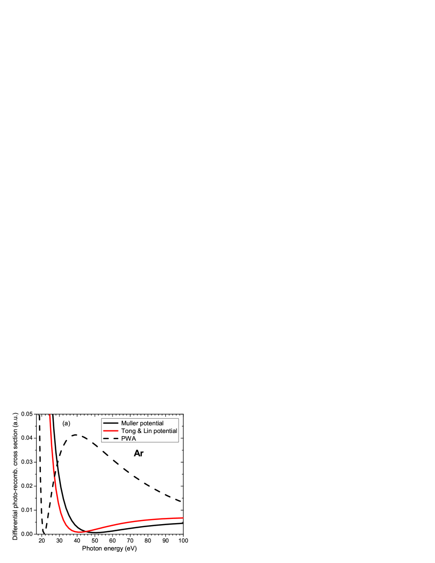
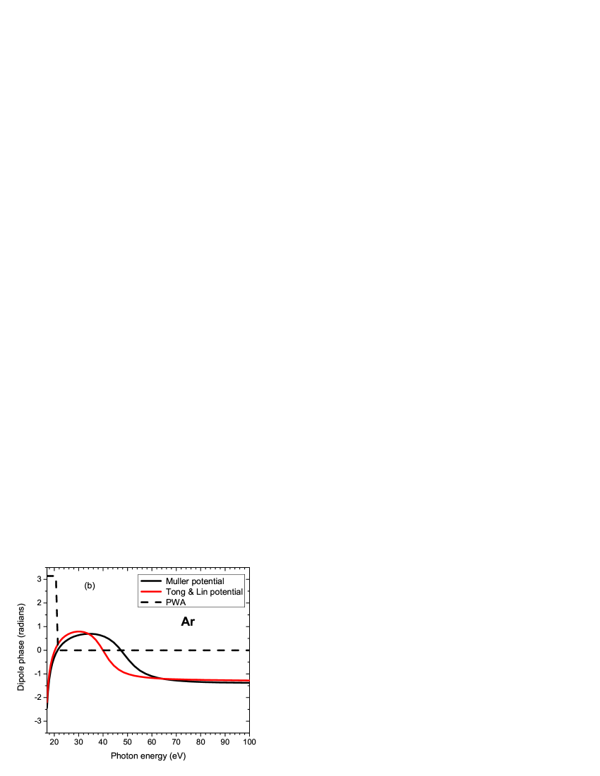
Figure 1: (Color online) Comparison of the differential photo-recombination cross sections (a) and dipole phases (b) from different models for Ar.

The simplicity of the model potential approach allows us to establish the validity of the QRS for atoms, by using the same potential in the TDSE and in the calculation of the photo-recombination transition dipole (see next subsection). In order to compare with experiments, one can go beyond the model potential approach by using different schemes to account for many-electron effect, i.e., final state and initial state correlation in photoionization (see, for example, starace ; lin74 ; amusia71 ). It is much harder to do so within the TDSE approach.

III.3 QRS for atomic targets: example of Argon

By using the photo-recombination cross section and dipole phase shown in the previous subsection, we are now ready to discuss the results from the QRS and assess its validity on an example of HHG from Ar(3p₀). We emphasize that in this paper we use a model potential proposed by Muller muller in order to get the Cooper minimum position comparable with experiments.

In Fig. 2(a) we show the comparison of the returning electron wave packets from both versions of the QRS with the “exact” wave packet, extracted from the solution of the TDSE for Ar by using Eq. (65). In the QRS2 the effective charge $Z_{eff}=1.0763$ is chosen such that the ionization potential from $1s$ state is 15.76 eV, the same as for Ar(3p₀). We use a 800-nm wavelength laser pulse with 8-cycle duration (8 fs FWHM) and peak intensity of $2.5\times 10^{14}$ W/cm². One can see very good agreement between QRS2 and the exact result over a very broad range of energy when the wave packet is extracted from the scaled atomic hydrogen. The result from the QRS1 (shifted vertically for clarity) with the wave packet from the SFA is also in reasonable good agreement with the exact one.

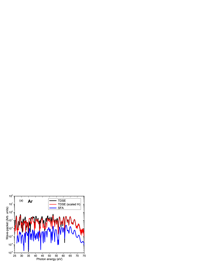
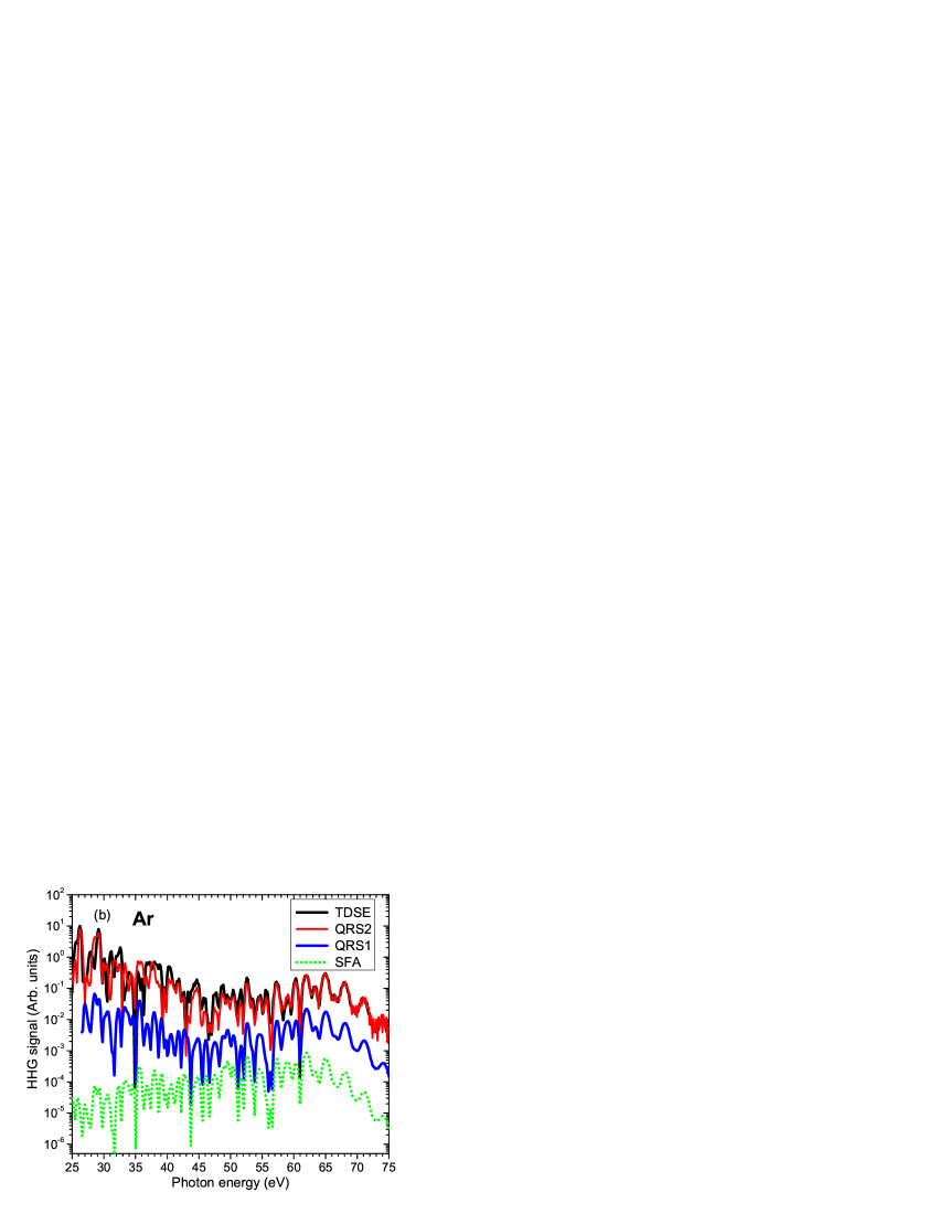
Figure 2: (Color online) (a) Comparison of the returning electron “wave packets” extracted from numerical solutions of the TDSE for Ar and scaled hydrogen and from the SFA for Ar. (b) Comparison of the HHG yields obtained from numerical solutions of the TDSE, QRS and SFA for Ar. Data have been shifted vertically for clarity. 8-cycle laser pulse with peak intensity of $2.5\times 10^{14}$ W/cm², 800-nm wavelength is used.

Fig. 2(b) shows comparison of the HHG yields from the TDSE, QRS1, QRS2 and the SFA. The data from QRS1 and SFA have also been shifted vertically for clarity. Clearly, the QRS results agree quite well with the TDSE, whereas the SFA result deviates strongly in the lower plateau. The signature of the Cooper minimum near 50 eV in the HHG spectra is quite visible. Note that the minimum has shifted as compared to the results reported in Ref. atle08 , which used a model potential suggested by Tong and Lin tong-jpb05 . The results in Fig. 2(b) clearly demonstrate the good improvement of the QRS over the SFA in achieving better agreement with the TDSE results.

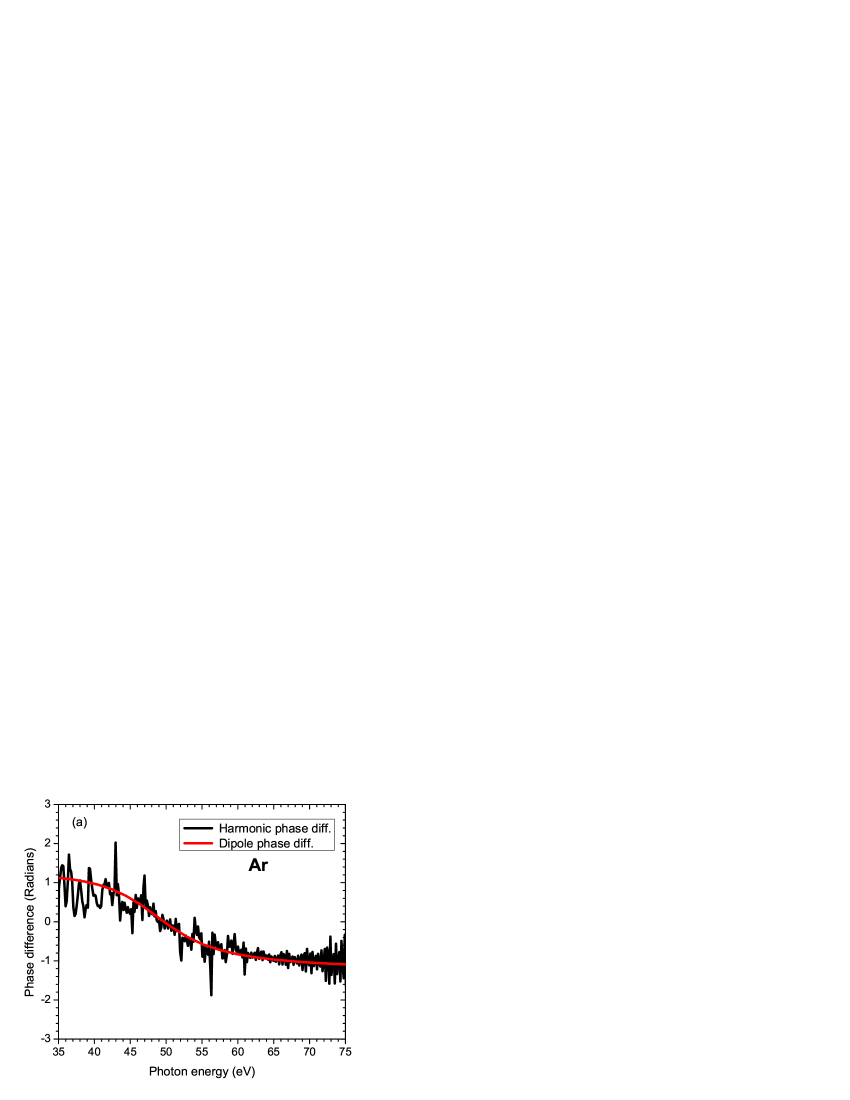
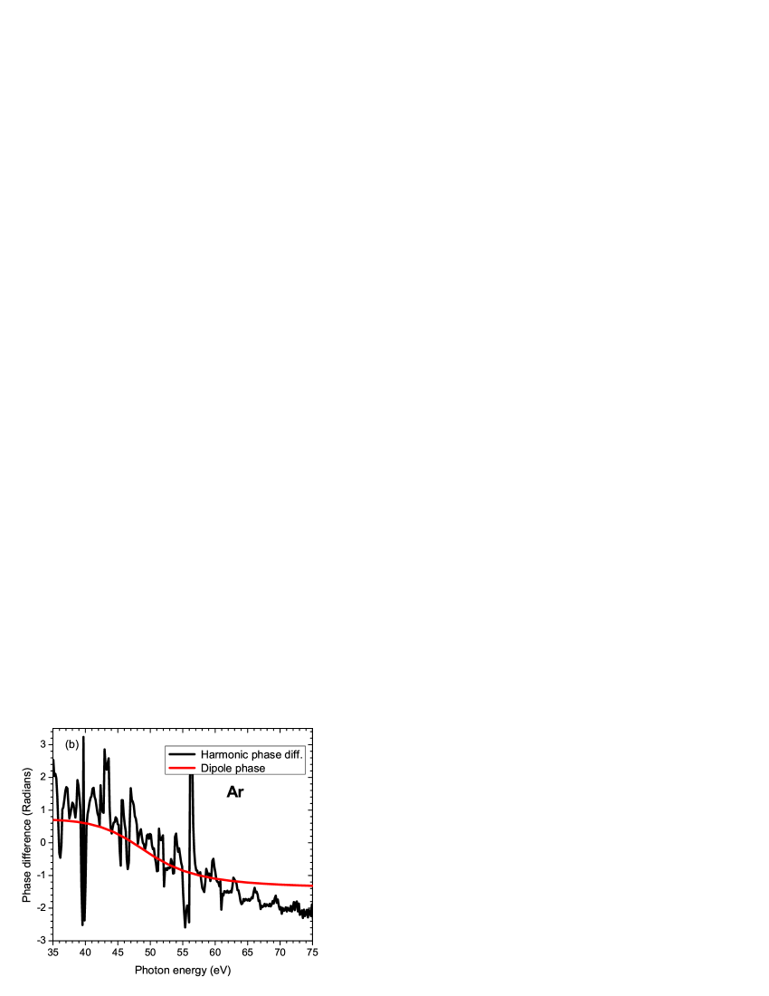
Figure 3: (Color online) (a) Comparison of extracted harmonic phase difference $\Delta\varphi$ between Ar and scaled hydrogen as a function of emitted photon energy with the photo-recombination transition dipole phase difference $\Delta\delta$. The results are obtained from numerical solutions of the TDSE. (b) Same as for (a), but SFA for Ar is used instead of a scaled hydrogen. Laser parameters are the same as for Fig. 2.

Next we examine harmonic phase, or induced dipole phase $\varphi$ [see Eq. (61)]. Since harmonic phase changes quickly from one order to the next (except in the harmonic cut-off), it is instructive to compare phases from different targets. For that purpose we calculate the harmonic phase difference $\Delta\varphi=\varphi-\varphi^{ref}$ of Ar from its reference scaled hydrogen. The result, shifted by 1.9 radians, is shown as the solid black curve in Fig. 3(a), at an energy grid with step-size of $0.1\times\omega_{0}$, where $\omega_{0}$ is the photon energy of the driving laser ($1.55$ eV). A striking feature is that this curve agrees very well with the transition dipole phase difference $\Delta\delta=\delta-\delta^{ref}$, shown as the red line. Since the transition dipole phase $\delta^{ref}$ from the reference scaled hydrogen is very small (about $0.2$ radians) in this range of energy, $\Delta\delta$ looks quite close to $\delta$ as well [see Fig. 1(b)]. Note the phase jump near the Cooper minimum at 50 eV is also well reproduced. This clearly demonstrates the validity of the QRS model in Eqs. (61) and (72) and with respect to the phase. The shift by 1.9 radians can be attributed to the phase difference of the two wave packets $\Delta\eta$, which is nearly energy independent.

Above result is based on the numerical solution of the TDSE for Ar and scaled hydrogen. Similarly one can compare the harmonic phase difference between the TDSE and SFA results $\Delta\tilde{\varphi}=\varphi-\varphi^{SFA}$ with that of the transition dipole phase $\Delta\tilde{\delta}=\delta-\delta^{PWA}$. Note that $\delta^{PWA}=0$ [see Fig. 2(b)]. Clearly, if the SFA and the PWA were exact, one would have $\Delta\tilde{\varphi}=\Delta\tilde{\delta}=0$. The results, presented in Fig. 3(b), show that the phase missed in the SFA is quite close to the transition dipole phase. The QRS1 therefore corrects the inaccuracy in the SFA phase by adding the phase from the transition dipole [see Eq. (68)]. By comparing Figs. 3(a) with 3(b), we conclude that the phase from QRS2 is more accurate than QRS1. This is expected since the QRS2 includes partially the effect of electron-core interaction during the propagation in the continuum, as explained in III(A).

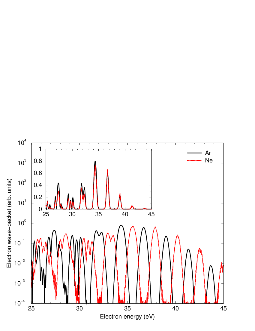
Figure 4: (Color online) The electron wave packets, extracted from the HHG spectra for Ne and Ar under the same laser field. The inset shows the wave packets in the linear scale with the Ne data shifted horizontally by -1.2 eV. The HHG are obtained within the Lewenstein model with 1064 nm laser, peak intensity of $2\times 10^{14}$ W/cm², duration of 50 fs.

Finally, we remark that the use of a reference atom with nearly identical ionization potential is not necessary. We will show here this requirement can be relaxed. As the wave packets obtained within the SFA agree reasonably well with the TDSE results, for our purpose we only use the SFA in the subsequent analysis. In Fig. 4, we show the comparison of the wave packet from Ne ($I_{p}=21.56$ eV) and Ar ($I_{p}=15.76$ eV) in the same 1064 nm laser pulse ($\omega=1.166$ eV) with peak intensity of $2\times 10^{14}$ W/cm², duration (FWHM) of 50 fs. Note that the wave packets are now plotted as functions of electron energy, instead of the photon energy as in Fig. 2(b). Clearly, the two wave packets lie nicely within a common envelope. This can be seen even more clearly in the inset, where the data are plotted in linear scale with the Ne data shifted horizontally by $-1.2$ eV. We note that the small details below 33 eV also agree well. This conclusion is also confirmed by our calculations with different laser parameters and with other atoms. This supports that the independence of the wave packet on the target structure can also be extended to systems with different ionization potentials. This fact can be useful in comparing experimental data for different targets. Note that the small shift of -1.2 eV is caused by the fact that the difference in the ionization potentials (5.8 eV) is incommensurate with the energy of two fundamental photons (2.3 eV).

III.4 Molecular photoionization cross sections and phases

Photoionization cross section and transition dipole phase from a linear molecule depend on both photon energy and angle between molecular axis and laser polarization direction. Since most interesting features of HHG from molecules are from molecules that have been pre-aligned by a pump laser pulse, it is more appropriate to present them as functions of fixed alignment angle for fixed energies. As noted before, one can use either photoionization or photo-recombination cross sections and phases in the QRS. Here we choose to use photoionization as it is in general more widely available theoretically and experimentally. In this paper we are only interested in the HHG with polarization parallel to that of the driving laser. That limits the differential cross sections to that case of ${\bm{k}}\parallel{\bm{n}}\parallel{\bm{n}}^{\prime}$ [see Eq. (65)].

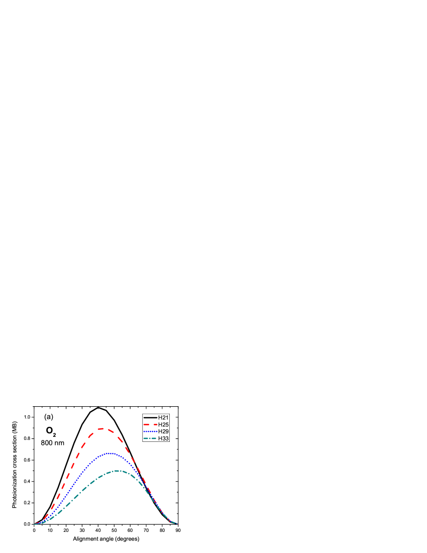
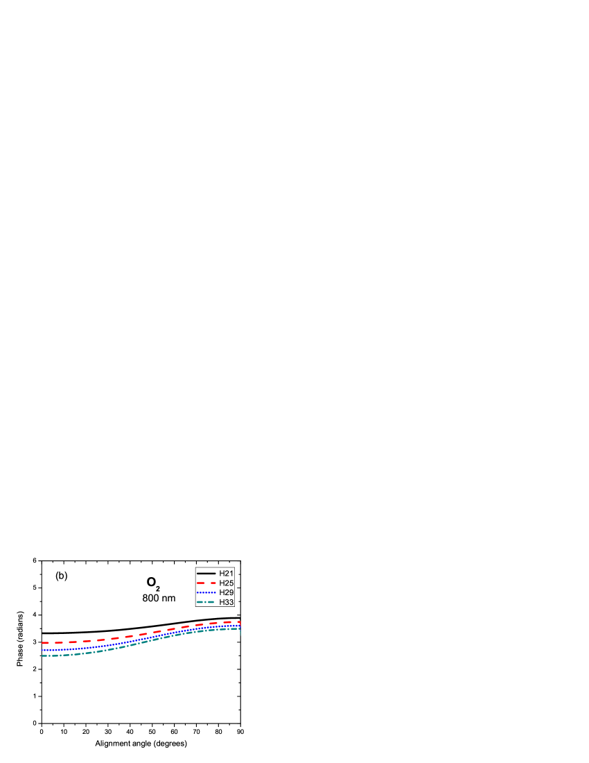
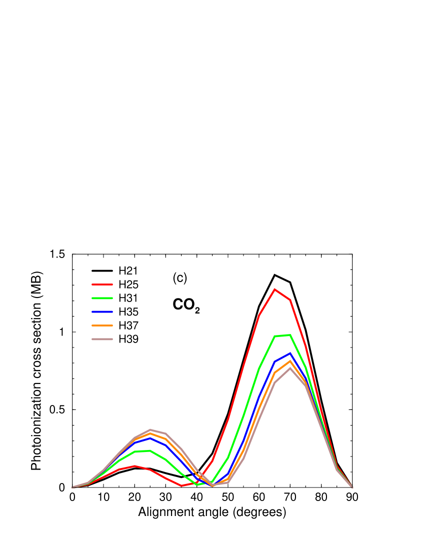
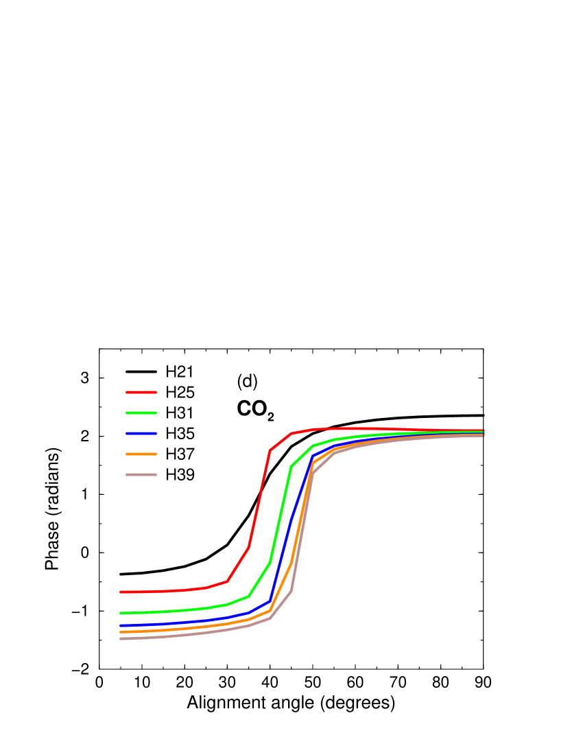
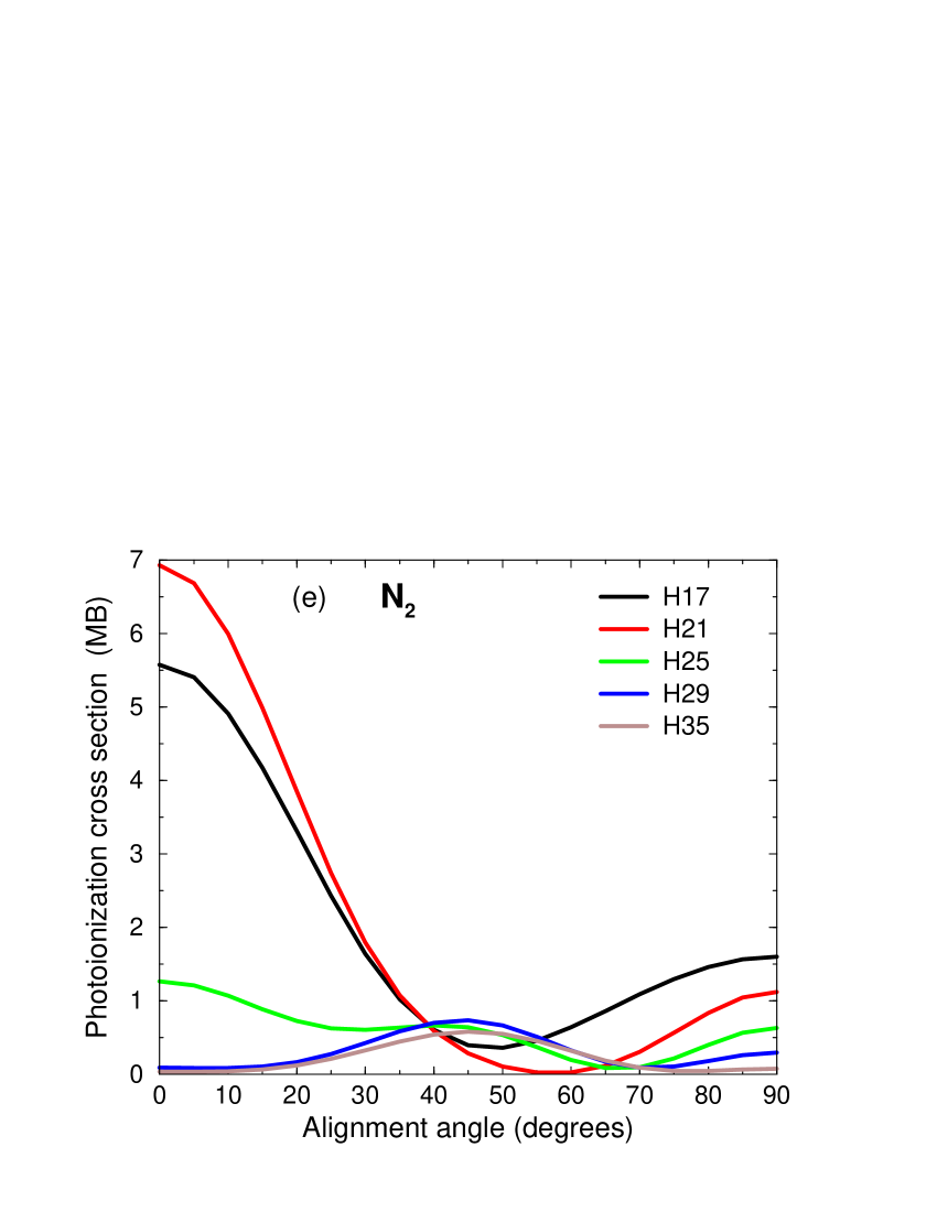
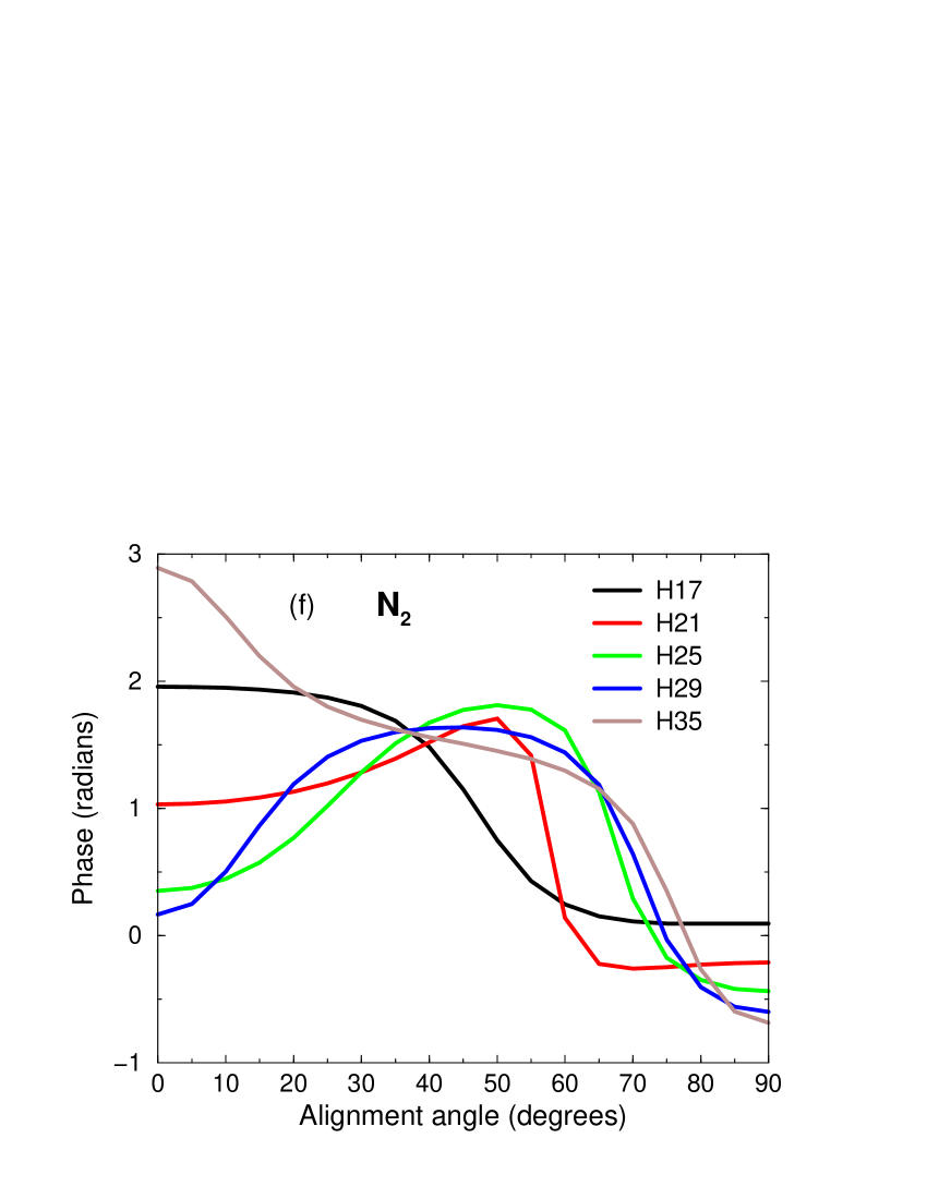
Figure 5: (Color online) Diffrential photoionization cross sections and transition phases for O₂, CO₂, and N₂, as functions of the alignment angle. The photon energies are expressed in units of harmonic orders for 800-nm laser.

The photoionization DCS and phase from O₂, CO₂, and N₂ are presented in Fig. 5(a-f) for some fixed energies as functions of angle between molecular axis and laser polarization direction. For convenience we express energy in units of photon energy of 800-nm laser. Let us first examine O₂, shown in Fig. 5(a) and (b). For a fixed energy the cross section vanishes at $\theta=0$ and $\pi/2$ due to the $\pi_{g}$ symmetry of the HOMO and the dipole selection rule for the final state and has a peak near $45^{\circ}$. As energy increases the peak slightly shifts to a larger angle and the cross section monotonically decreases. The phases behave quite smoothly and change only within about 1 radian for all energies considered. For CO₂, the cross section also vanishes at $\theta=0$ and $\pi/2$ due to the $\pi_{g}$ symmetry of the HOMO. However in contrast to O₂, for a similar range of energy the DCS of CO₂ shows a double-hump structure with the minimum shifting to a larger angle as energy increases. These features can also be seen in the phase of the transition dipoles [Fig. 5(d)], where the phase jump by almost $\pi$ is observed near the minima in the cross section. The two “humps” also behave quite differently. Within the range of energy from H21 to H39, the small hump at small angles increases and the big hump at large angles decreases with increasing energy. We note that the phase jump is smaller than $\pi$ as the cross section does not go to zero at the minimum between the two humps. In this paper we will limit ourselves to application of the QRS to O₂ and CO₂. Nevertheless it is worthwhile to point out that the case of N₂ is even more complicated than CO₂, with almost no regular behavior found in the energy range presented here, see Fig. 5(e) and (f). Note that the sharp variation of cross section from H17 to H25 is due to the presence of the well-known shape resonance in N₂. The shape resonance is accompanied by a rapid phase change in the same energy region.

We have seen that these three molecular systems behave totally differently in photoionization. We show in Sec. IV that such differences can be seen from the HHG spectra.

III.5 Wave packets from molecular targets: example of O₂

In subsection III(C) we have shown evidence to validate the QRS for atomic targets. For molecular targets some benchmark TDSE results are available only for H${}_{2}^{+}$ lein04 ; kamta05 ; telnov07 . In fact successful application of the QRS and detailed comparisons with the TDSE results for this system has been reported in H2+ . In this subsection for completeness we show here an example of the wave packets from O₂ and Xe, which have nearly identical ionization potentials (12.03 eV for O₂ and 12.13 eV for Xe). In Fig. 6(a) we compare the HHG spectra from O₂ aligned at 10^∘ and 70^∘, with that from Xe. These results were obtained from the SFA, with 1600 nm laser of $1\times 10^{14}$ W/cm² intensity and 20 fs duration (FWHM). The long wavelength is used here in order to compare the wave packets in the extended HHG plateau. Clearly, the HHG spectra look quite different. However, the wave packets, extracted by using Eqs. (67) and (70), shown in Fig. 6(b) are almost identical. For clarity we have shifted the curves vertically in both Figs. 6(a) and (b). The QRS results for the HHG are shown in Fig. 6(c). The changes in the slope of the QRS yields as compared to that of the SFA in Fig. 6(a) can be easily seen, which reflects the differences of the exact and the PWA photoionization DCS.

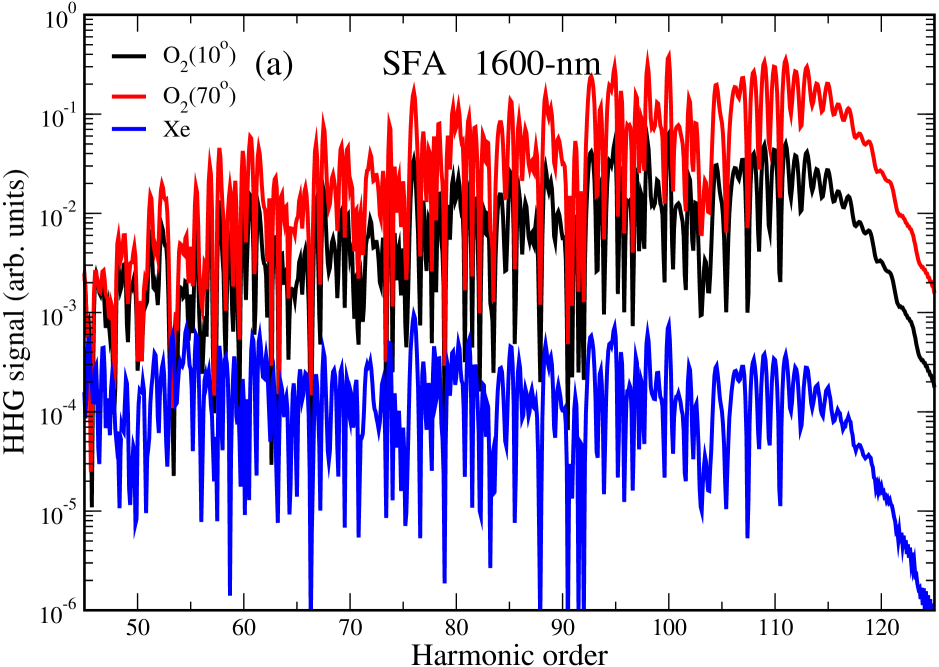
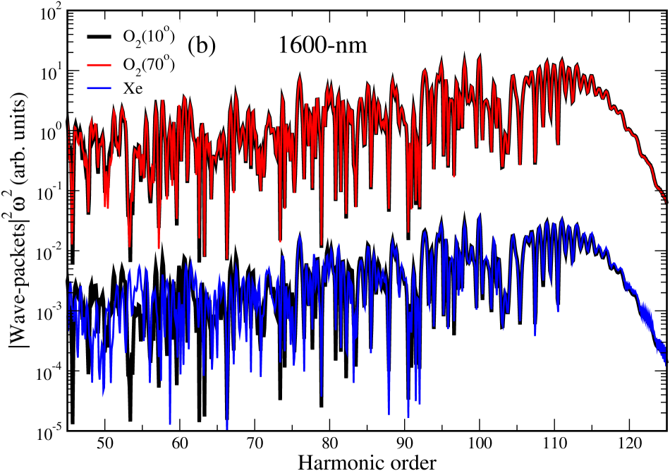
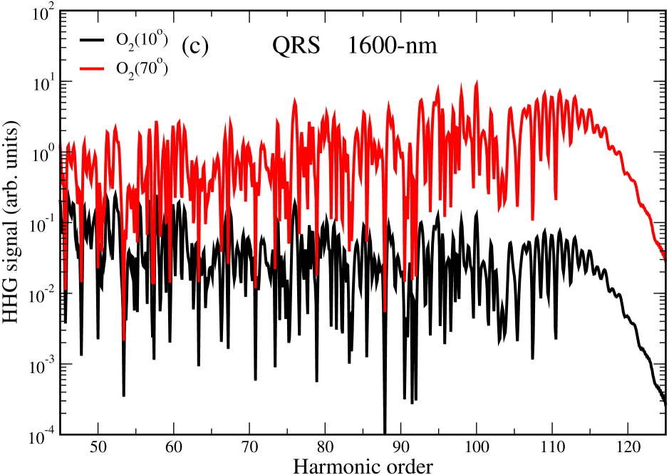
Figure 6: (Color online) (a) Comparison of the HHG spectra obtained from the SFA for O₂ aligned at 10^∘ and 70^∘, and Xe under laser pulse with wavelength of 1600 nm, intensity of $1\times 10^{14}$ W/cm² and duration of 20 fs. For clarity, we have shifted Xe data vertically. (b) Comparison of the electron returning wave packets extracted from (a). Wave packet for O₂ at 10^∘ is renormalized to that of 70^∘ and Xe and plotted twice. (c) The HHG spectra from O₂ aligned at 10^∘ and 70^∘ from the QRS.

This example clearly shows that in order to calculate the HHG spectra for a fixed alignment within the QRS one can use the wave packet from any other alignment angle or from a reference atom, with an overall factor accounting for the differences in tunneling ionization rates [see Eq. (66)]. This feature enables us to avoid the possible difficulties associated with direct extraction of the wave packet at the energies and alignments where the transition dipole in the PWA vanishes. For example, in case of N₂, it is more convenient to use the wave packet extracted for alignment angle of $90^{\circ}$, as the transition dipole in the PWA does not vanish. Furthermore, if a reference atom is used, one can also extract the wave packet from the solution of the TDSE, as has been done for H${}_{2}^{+}$ H2+ .

IV Comparisons with experiments

In this section we will compare the QRS results with the recent HHG measurement from partially aligned molecules. Below we will look at two examples of molecular O₂ (with internuclear distance at equilibrium $R=2.28$ a.u.) and CO₂ ($R=4.38$ a.u. between the two oxygen centers), which can also be seen as “elongated” O₂. HHG from aligned molecules are typically measured experimentally with the pump-probe scheme. In this scheme, non-adiabatic alignment of molecules is achieved by exposing them to a short and relatively weak laser pulse (the pump) to create a rotational wave packet. This wave packet rephases after the pulse is over and the molecules are strongly aligned and anti-aligned periodically at intervals separated by their fundamental rotational period seideman . To observe the alignment dependence of HHG, a second short laser pulse (the probe) is then used to produce HHG at different short intervals when the molecules undergo rapid change in their alignment. A slightly different setup is done by changing the relative angle between the pump and probe polarizations, but measure the HHG at fixed time delays, typically at maximal alignment (or anti-alignment) near half-revival. Theoretically, induced dipoles from the QRS need to be calculated first for a fixed molecular alignment. The results will then be convoluted with the molecular distribution following the theory presented in Sec. II(F).

IV.1 HHG from aligned O₂ molecules

In Sec. III(D) we showed harmonic spectra generated with 1600-nm laser. This was used in order to compare the wave packets in an extended plateau. To compare with available experiments calculations in this subsection are performed with 800-nm laser. First we show in Fig. 7(a) the HHG yields for some selected harmonics for fixed molecular axis. Calculations are done with the QRS, for a 30-fs pulse with a peak intensity of $2\times 10^{14}$ W/cm². The yields are maximal if molecules are aligned at about $45^{\circ}$ with respect to the probe polarization, and vanish at $0^{\circ}$ and $90^{\circ}$ due to $\pi$-symmetry of the HOMO. This result resembles closely the behavior of the photoionization DCS’s shown in Fig. 5(a), but with the relative magnitudes changed, reflecting the influence of the returning wave packets. The yields convoluted with the partial distribution with maximally aligned ensemble at half-revival are shown in Fig. 7(b), as functions of relative angle between pump and probe polarizations. Interestingly, the yields are now peaked near $0^{\circ}$, that is, when the pump and probe polarizations are parallel. This result is consistent with the data by Mairesse et al mairesse08 (see their Fig. 2) and with the earlier measurements by Miyazaki et al miyazaki05 . Note that the yield is quite insensitive to the alignment angle. However, the contrast can be increased with a better alignment. Our simulations for alignment are carried out using the pump laser intensity of $5\times 10^{13}$ W/cm² and 30 fs duration, with a rotational temperature of 30 K, the same as used in the experiment. We note that the convoluted yields from the earlier SFA results by Zhou el al zhou05b show peaks near $45^{\circ}$ with similar laser parameters. Within the QRS we found that only with higher degrees of alignment the peaks shift to about $45^{\circ}$. This can be achieved, for example, with the same pump laser intensity, but with a longer duration.

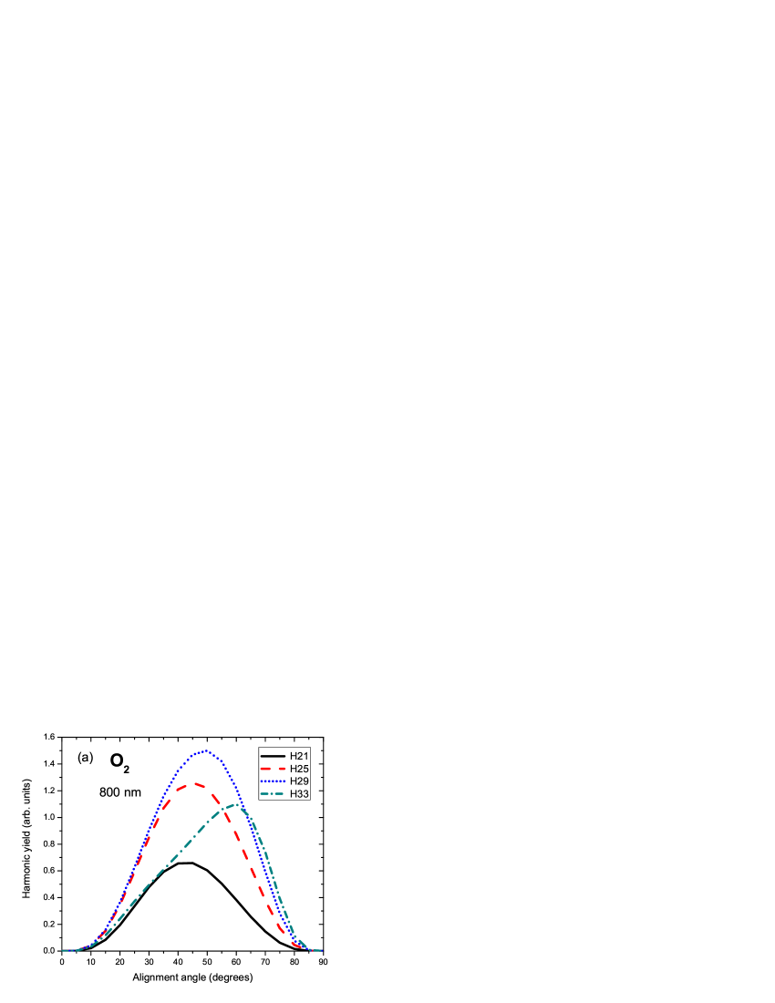
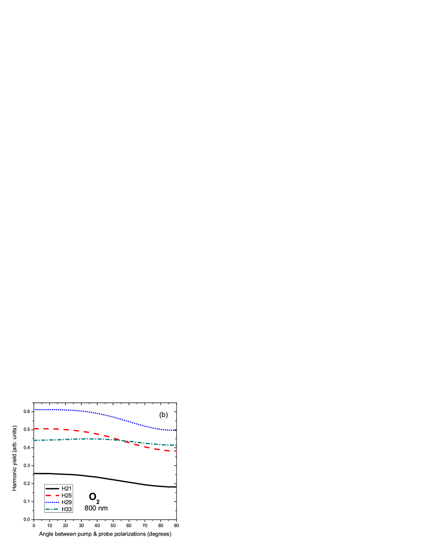
Figure 7: (Color online) Alignment dependence of harmonic yields from O₂ harmonics H21, H25,H29, and H33 for fixed molecular axis (a) and convoluted with molecular alignment distribution (b).

Next we compare in Fig. 8 harmonic yields from H17-H35 as a function of delay time near quarter- and half-revivals from the QRS and the SFA calculations with the experiments by Itatani et al itatani05 . Calculations were done with laser parameters taken from Ref. itatani05 and the yields have been normalized to that of the isotropic distribution. Clearly both theories reproduce quite well the behavior of the experimental curve, which follows $<\sin^{2}2\theta>$, shown in the upper panel. A closer look reveals that the QRS result agrees better with the experiment and the SFA tends to overestimate the yield near maximal alignment and underestimates it near maximal anti-alignment. In fact, similar quantitative discrepancies between the SFA and experiments can be seen in an earlier work by Madsen et al madsen06 for both O₂ and N₂. Note that the discrepancies between the simulations and the experiment along the delay time axis could be due to inaccuracy in the determination of laser intensities and temperature used in the experiment.

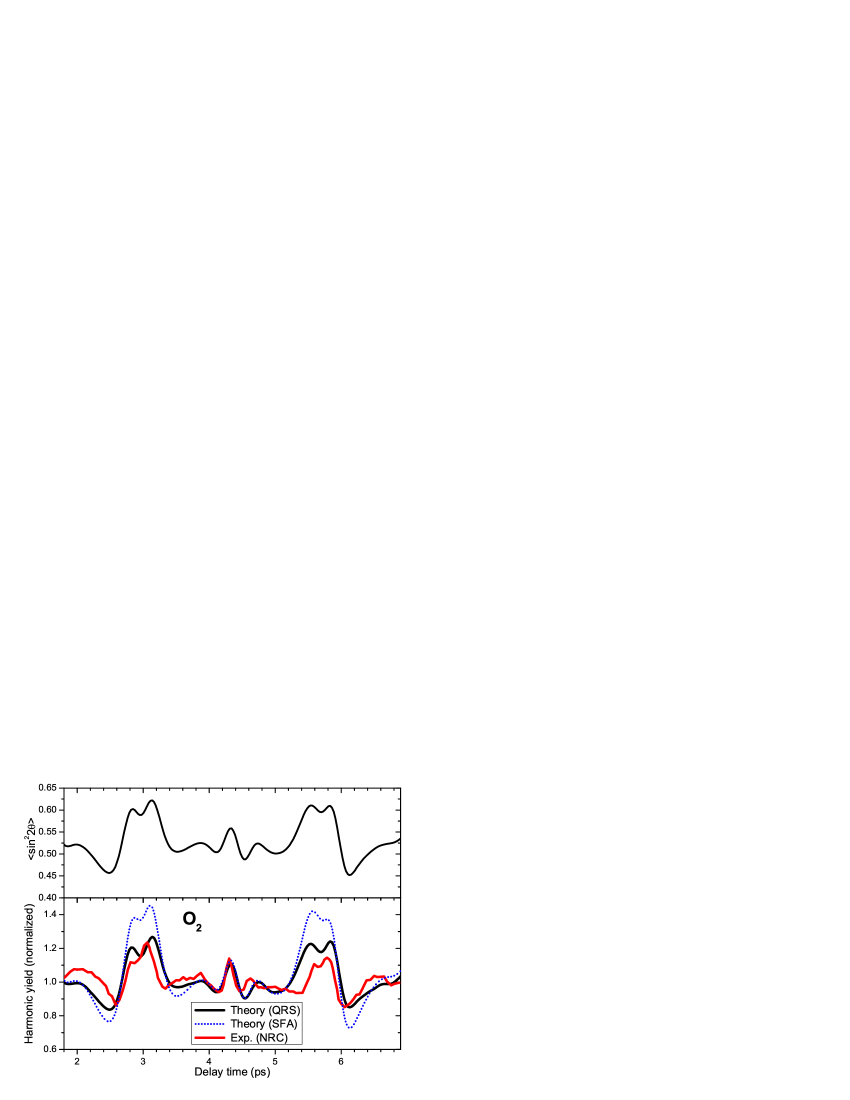
Figure 8: (Color online) Comparison of O₂ time evolution of (normalized) harmonic yields H17-H35 from the QRS, SFA and experiment, near quarter and half-revivals. The experimetal data and laser parameters are taken from Itatani et al itatani05 . $<\sin^{2}2\theta>$ is shown in the upper panel for reference.

We have seen so far only quantitative improvements of QRS over the SFA for O₂. The situation is completely different for CO₂, presented in the next subsection, where the two theories predict qualitatively different results.

IV.2 HHG from aligned CO₂ molecules

First we show in Fig. 9(a) theoretical HHG yields for selected harmonics from H21 up to H39, obtained from the QRS for fixed angles between the molecular axis and the polarization of the probe pulse. The yields resemble closely the photoionizations DCS of Fig. 5(c), with the double-hump structures seen quite clearly for the higher harmonics above H31. For the lower harmonics, the smaller humps nearly disappear. To compare with experiment, average over the molecular alignment needs to be performed. We take the alignment distribution for a pump-probe delay time at the maximum alignment near half-revival. The convoluted yields are presented in Fig. 9(b), as functions of the angle between the pump and probe polarizations. Clearly, due to the averaging over the molecular alignment distributions, the angular dependence of HHG is smoother as compared to fixed alignment data in Fig. 9(a). These results are consistent with recent experiments boutu ; mairesse08 ; jila-private , which show enhanced yields for large alignment angles and minima near $30^{\circ}$ for harmonics above H31. We note that our results also resemble the data for the induced dipole retrieved from mixed gases experiments by Wagner et al. jila07 (see their Fig. 4). To have a more complete picture of the HHG yields, we show in Fig. 9(c) a false-color plot of HHG yield as a function of harmonic orders and the angle between the pump and probe lasers polarization directions, at the delay time corresponding to the maximum alignment near the half-revival. Clearly the yield has quite pronounced peak at large alignment angle. However, the most pronounced feature in Fig. 9(c) is a minimum at small angles, which goes to larger angles as with increasing harmonic orders. Within the QRS the origin of this minimum can be directly traced back as due to the minimum in the photo-recombination DCS’s. Our results are comparable with the recent measurement by Mairesse et al mairesse08 (see their Fig. 2), which were carried out with a slightly different laser parameters. Interestingly, our results resemble closely with the theoretical calculations by Smirnova et al smirnova09 , which include contributions from the HOMO, HOMO-1 and HOMO-2 orbitals [see their Fig. 1(b), plotted in a x-y plot]. In our calculations, only the HOMO is included. We note that the position of the minima can be slightly shifted depending on the actual experimental laser setup. The above calculations for HHG were done with a 25-fs probe laser pulse with intensity of $2.5\times 10^{14}$ W/cm². Alignment distribution was obtained following the method is Sec. II(F), with a $120$-fs pump laser pulse with intensity of $0.55\times 10^{14}$ W/cm². Rotational temperature is taken to be $105$ K. These parameters are taken from the recent experimental setup by Zhou et al jila08 .

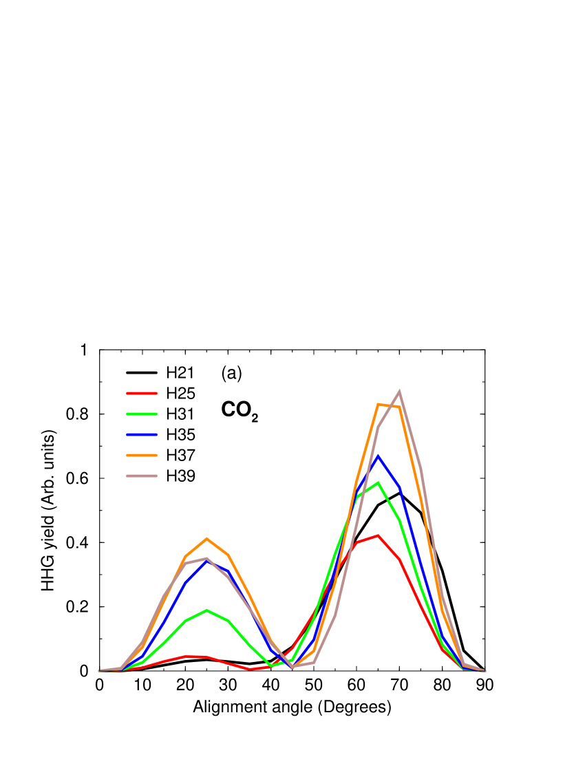
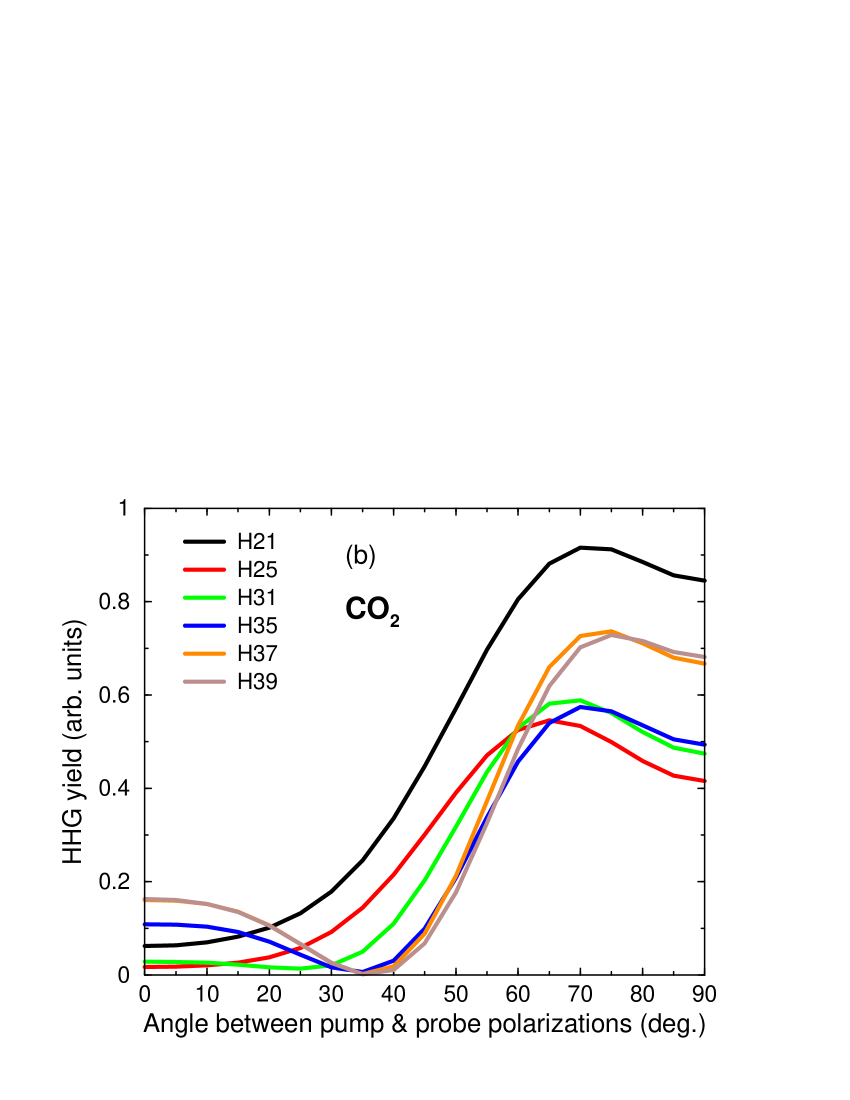
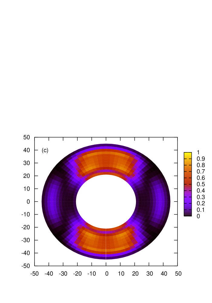
Figure 9: (Color online) HHG yield as a function of fixed angle between molecular axis and laser polarization (a) and as a function of angle between pump and probe laser polarization directions (b). False-color plot of HHG yield for a harmonic range between H20 and H42 (c). In (c) the probe laser is horizontally polarized. Alignment distribution is chosen at the maximum alignment near half-revival. The laser intensity and duration are of $0.55\times 10^{14}$ W/cm², and $120$ fs for the pump pulse, and $2.5\times 10^{14}$ W/cm² and $25$ fs for the probe pulse. Rotational temperature is taken to be $105$ K.

Comparison of theoretical HHG amplitudes for a few angles between pump and probe polarizations from $0^{\circ}$ to $25^{\circ}$ is shown in Fig. 10(a) together with the experimental data in Fig. 10(b), taken from Mairesse et al mairesse08 . The experimental data have been renormalized to a smoothed experimental wave packet from Ar under the same laser field. This wave packet is a decreasing function of harmonic order, therefore the renormalized signals in Fig. 10(b) are enhanced at higher orders compared to lower orders. No such renormalization was done for the theoretical data. Nevertheless, reasonably good agreement with the experimental data can be seen, including the shift of the minimum position to higher harmonics as alignment angle increases. The theoretical data seem to have more structures than the experimental ones. That might be due to the fact that that we use a single intensity, single molecule simulation. It is known that macroscopic propagation in general tends to smooth out the HHG spectra.

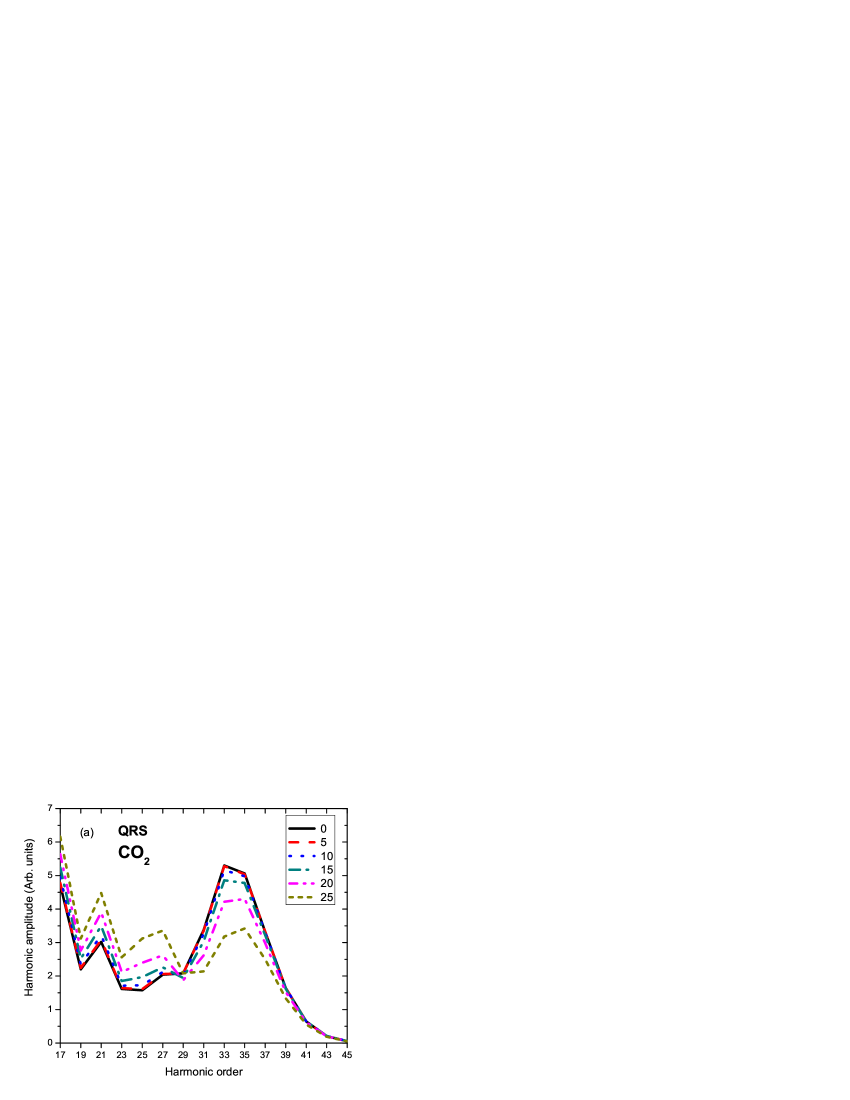
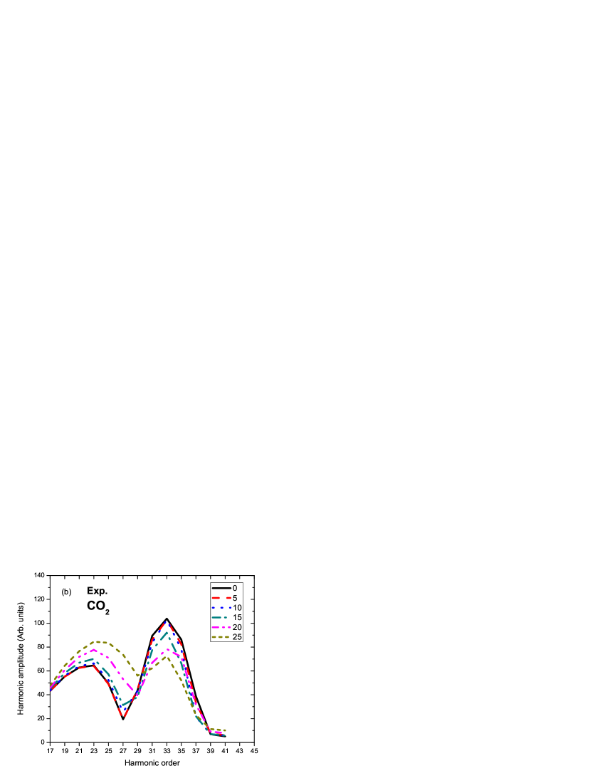
Figure 10: (Color online) Harmonic amplitudes for CO₂ for a few angles from $0^{\circ}$ to $25^{\circ}$. The experimental data by Mairesse et al mairesse08 are also shown for comparison (b). The experimental data have been renormalized to a smoothed experimental wave packet from Ar under the same laser field.

As found in Zhou et al jila08 , the most dramatic feature can be seen near 3/4-revival, where the molecule can be most strongly aligned. Our QRS results are shown in Fig. 11 for the same harmonics that have been analyzed in jila08 (see their Fig. 2). (We note here that according to the authors of jila08 , the harmonic orders should be properly shifted down by two harmonic orders, as compared to the ones given in their original paper). Theoretical results were carried out with laser parameters taken from jila08 . As can be seen from our results for the lower harmonics H21 and H25, the yields follow the inverse of the alignment parameter $\langle\cos^{2}\theta\rangle$, shown in Fig. 11(a). However, for the higher harmonics, an additional peak appears right at the delay time corresponding to the maximum alignment. The peak starts to appear near H31 and gets more pronounced with increasing harmonic orders. This behavior is in quantitatively good agreement with the measurements by Zhou et al. jila08 . In Zhou et al, the experimental data were fitted to the two-center interference model, by using a three-parameter least-square fitting procedure. Within the QRS, no fitting is needed. Furthermore, one can trace back the origin of the time-delay behavior based on the two-hump structure of the photoionization DCS. Indeed, Fig. 5(b) shows that for the lower harmonics H21 and H25 the cross sections at large angles are much larger than at small angles so the HHG yield is inverted with respect to $\langle\cos^{2}\theta\rangle$, for which small angles dominate. This fact has been known before atle06 . For the higher orders, Fig. 5(b) indicates that the smaller hump at small angles become increasingly important. Qualitatively, this explains why the HHG yields for H31 and up show a pronounced peak for the parallel alignment. In fact, it is even more simpler to explain this behavior by looking directly at the HHG yields shown in Fig. 9(a). One can immediately notice that the peak at small angles near $25^{\circ}$ starts to show up more clearly only near H31. We note that apart from the additional peaks, which are clearly visible at 3/4-revival, the general behavior of all harmonics from H19 up to cutoff near H43 shows inverted modulation with respect to $\langle\cos^{2}\theta\rangle$. Therefore, in contrast to the interpretation of Kanai et al kanai05 , inverted modulation is not an unambiguous indication of the interference minimum, especially for determining the precise position of the minimum.

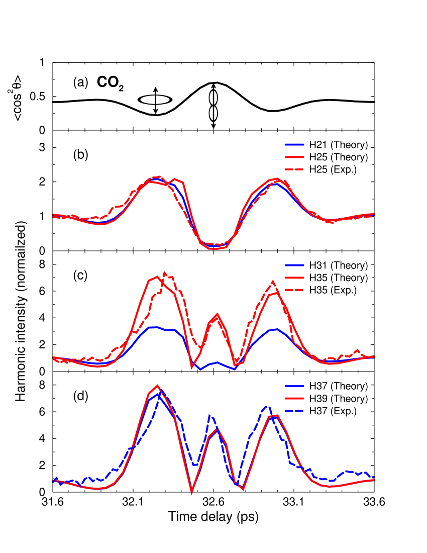
Figure 11: (Color online) Normalized HHG yield (vs isotropically distributed molecules) from CO₂ for selected harmonics as function of pump-probe delay time near 3/4-revival. The experimental data are taken from Zhou et al jila08 . Theoretical results were obtained with laser parameters taken from jila08 . The alignment parameter $\langle\cos^{2}\theta\rangle$ is also plotted for reference in the top panel.

Since the laser intensity in the experiment is quite high, the depletion of the ground state needs to be accounted for atle06 ; atle07 ; xu08 . Therefore discussion about the ionization rate is in order. Alignment dependence of the ionization rate for CO₂ is still a subject of debate. In our previous attempts atle06 ; atle07 , the MO-ADK theory moadk has been used to calculate the ionization rate. The MO-ADK theory predicts the peak in ionization rate near $30^{\circ}$, in agreement with the results deduced from measured double ionization KSU-exp . The recent experiment by the NRC group NRC-exp , however, show very narrow peak near $45^{\circ}$. Interestingly, the MO-SFA predicts a peak near $40^{\circ}$. However the MO-SFA theory is known to underestimate the ionization rate. In order to correct the MO-SFA rate, we renormalize the MO-SFA rate to that of the MO-ADK rate at laser intensity of $10^{14}$ W/cm², which gives a factor of $10$. Note that the same correction factor has been found for the SFA ionization from Kr, which has almost the same ionization potential as for CO₂. With the corrected MO-SFA rate, we found that our simulations give a better quantitative agreement with the JILA data, than with the MO-ADK rate. On the other hand, calculation with the uncorrected rate would lead to much more pronounced peaks right at the maximum alignment near 32.6 ps for H31 and higher harmonics.

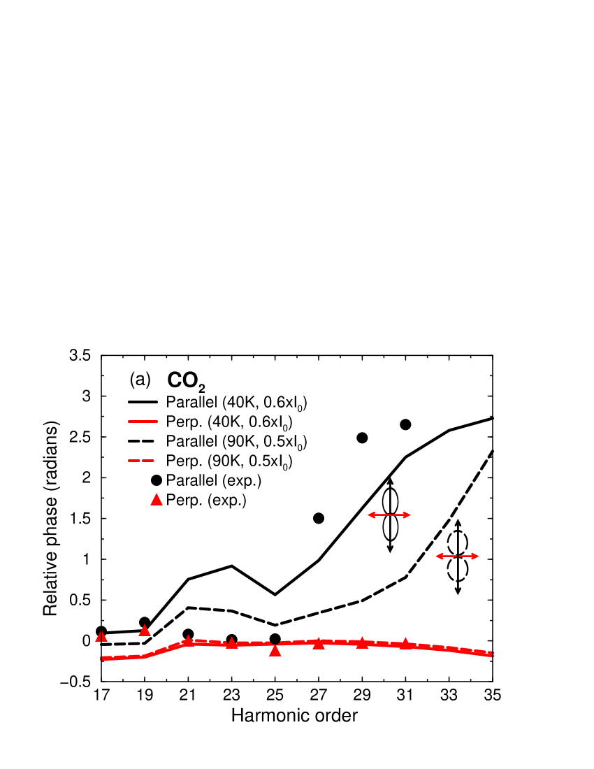
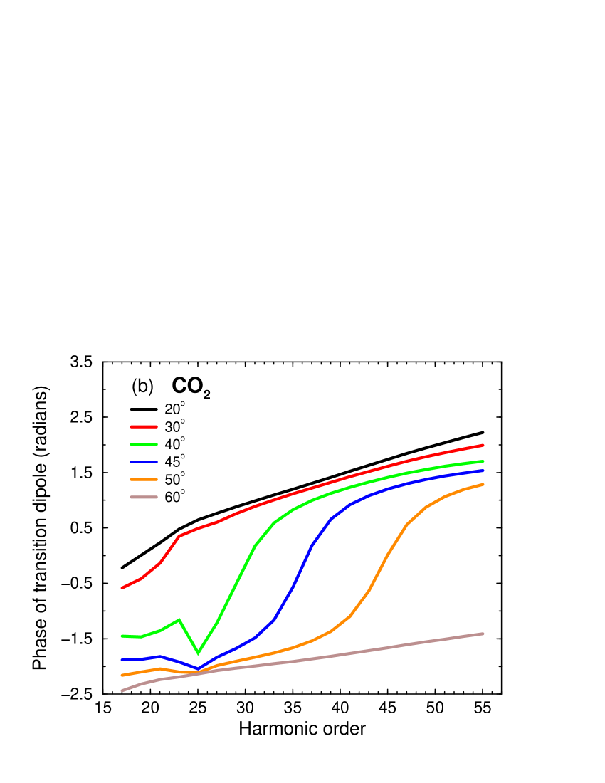
Figure 12: (Color online) (a) Harmonic phase (relative to the phase from Kr) for parallel aligned and perpendicular aligned ensembles, under two sets of parameters (solid and dashed lines) that lead to two different degrees of alignment distributions. Experimental data from Boutu el al. boutu are shown as symbols. Calculations are carried out with the same probe laser parameters as in the experiments. (b) Phase of the transition dipole for alignment angles from $20^{\circ}$ to $60^{\circ}$.

We next compare the predictions of the QRS for harmonic phase with experiments. The phase information can be of great importance. In particular it has been suggested as a more accurate way to determine positions of interference minima in HHG spectra. Experimentally the harmonics phase can be extracted from measurements of HHG using mixed gases boutu ; riken08 or interferometry method jila08 . In Fig. 12(a), we show the recent experimental data of Boutu et al. boutu where the harmonics phases (relative to that from Kr) are obtained for the parallel aligned and perpendicularly aligned ensembles, shown by black and red symbols, respectively. For the latter, the phase does not change much within H17 to H31. For the parallel aligned molecules, the phase jump from H17 to H31 was reported to be $2.0\pm 0.6$ radians. Our simulations are shown for two different ensembles, with alignment distributions confined in a cone angle of $~{}25^{\circ}$ (solid lines) and $35^{\circ}$ (dashed lines) at half maximum. The less aligned ensemble was obtained with the pump laser parameters and rotational temperature suggested by Boutu et al boutu . For the perpendicularly aligned molecules, the relative phase from both ensembles are almost identical and nearly independent of harmonic orders. This is in good agreement with the experiment. For the parallel case, our result with the pump laser parameters suggested in boutu shows the phase jump starting near H31, which only mimics the experimental data. However, the phase jump slightly shifted to near H27 with the better aligned ensemble (solid line), bringing the result closer to the experiment. This indicates that the degree of alignment can play a critical role in determination of the precise position of the phase jump. A possible reason for the discrepancy is that the experimental setup was chosen such that the short trajectory is well phase-matched, whereas our simulations are carried out at the single molecule level with contributions from both long and short trajectories. In order to understand the origin of the phase jump and its dependence on degree of alignment, it is constructive to analyze transition dipole phase as a function of harmonic order for fixed alignments. This is shown in Fig. 12(b) for angular range from $20^{\circ}$ to $60^{\circ}$. Clearly, the dipole phase shows a phase jump which shifts to higher order with larger angle. With a better alignment more contribution comes from small angles and the phase jump shifts toward smaller harmonic orders. Our calculations are carried out with a relatively low probe laser intensity of $1.25\times 10^{14}$ W/cm², the same as used in Boutu et al experiments boutu , in order to keep ground state depletion insignificant. As probe intensity increases our results indicate that the phase jump slightly shifts toward higher harmonic orders. Note that the phase jump cannot be reproduced within the SFA, where the insignificant phase difference between CO₂ and Kr is caused only by the small difference in their ionization potentials (13.77 eV vs 14 eV), independently of alignment.

V Validity of the Two-center interference model

Within the QRS theory, the structure of the HHG spectra directly relates to photo-recombination cross section. In particular, minima in photo-recombination cross section immediately result in minima in HHG spectra. It is therefore interesting to compare the positions of the minima in molecular systems under consideration with the prediction of the simple two-emitter model by Lein et al lein02 . According to this simple model, the minima satisfy the relation

$$R\cos\theta = (n+1/2)\lambda^{eff},\quad n=0,1,2,...,\quad\mbox{symmetric wavefunction},$$ (74)

$$= n\lambda^{eff},\quad n=1,2,...,\quad\mbox{anti-symmetric wavefunction}$$ (75)

where $\lambda^{eff}$ is the “effective” wavelength of the continuum electron defined such that the “effective” wave vector is $k^{eff}=\sqrt{2\Omega}$ , with $\Omega$ being the energy of the emitted photon. In other words, the energy is shifted by $I_{p}$ with respect to the usual relation $k=\sqrt{2(\Omega-I_{p})}$.

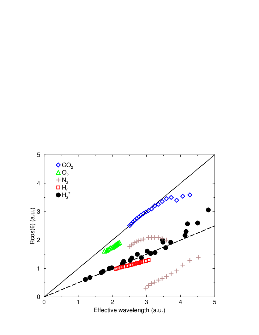
Figure 13: (Color online) Projected internuclear distance vs electron “effective” wavelength at the minima of the photoionization differential cross sections for CO₂, O₂, N₂, and H₂. Results for H${}_{2}^{+}$ with different internuclear separations, reported in Ref. H2+ , are also plotted for comparison. Predictions of the two emitter model are shown as dashed and dotted lines for symmetric and anti-symmetric wavefunctions, respectively.

In Fig. 13 we show the projected internuclear distance $R\cos\theta$ vs electron “effective” wavelength at the minima of the photoionization differential cross sections for CO₂, O₂, N₂, and H₂. For completeness, we also plot here the results for H${}_{2}^{+}$ with different internuclear separations, reported in Ref. H2+ . Remarkably, the minima from CO₂ follow the two-emitter model very well, shown as the dotted line for the case of anti-symmetric wavefunction (due to the $\pi_{g}$ symmetry of the HOMO). This fact has been first observed experimentally in the HHG measurement from aligned CO₂ kanai05 ; vozzi05 , and more conclusive evidences have been shown in Ref. jila08 ; riken08 ; boutu . For O₂, which also has the $\pi_{g}$ symmetry for the HOMO, the minima start to show up only at quite high energies (or shorter wavelengths). This is not surprising since the internuclear distance between the two oxygens is about two times shorter, as compared to CO₂. The case of H₂ also agrees reasonably well with the two-emitter model. However, N₂ minima do not follow any simple pattern. This fact has been noticed earlier by Zimmermann et al zimmermann . This clearly indicates that the two-center interference model is not guarantied to work a priori.

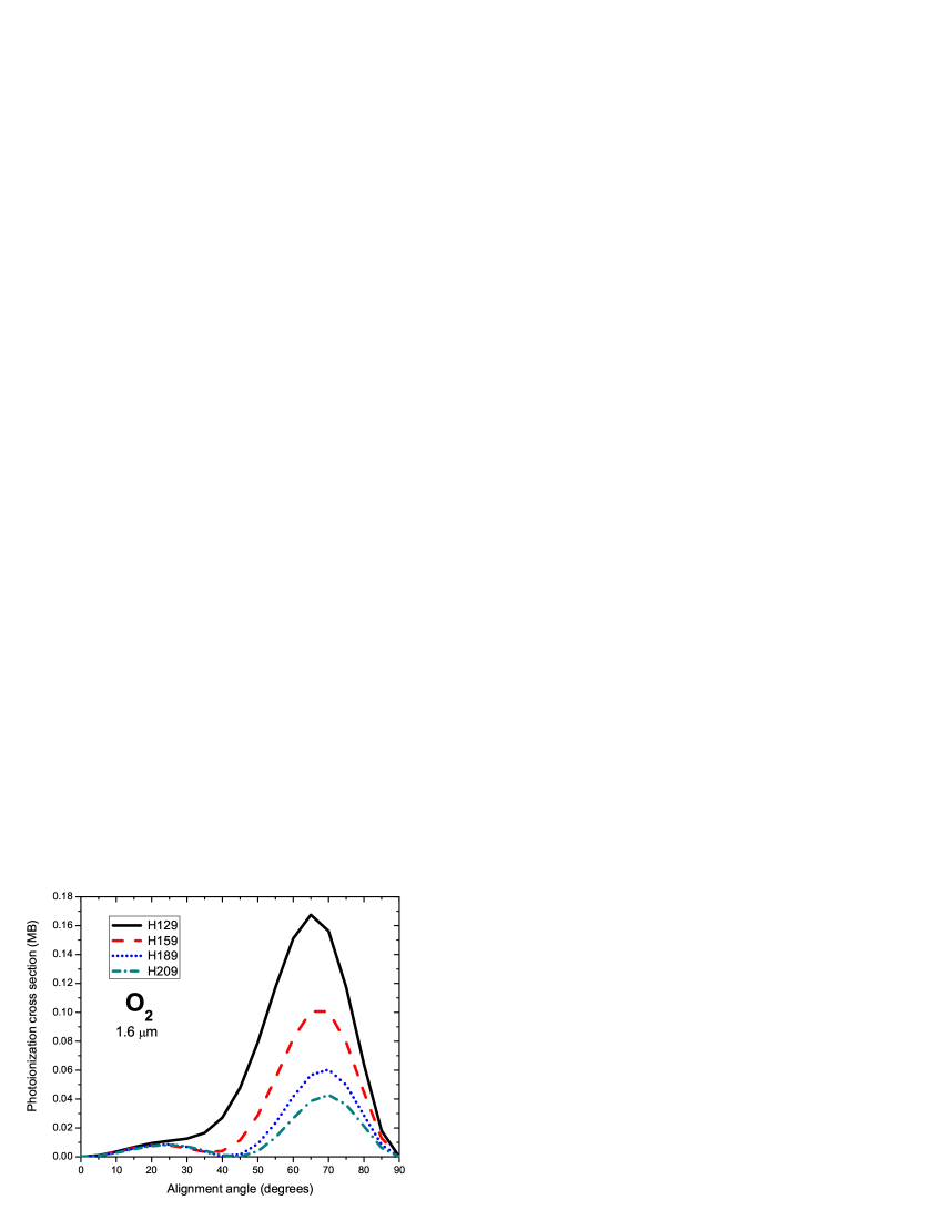
Figure 14: (Color online) Diffrential photoionization cross sections for O₂ as functions of the alignment angle. The photon energies are expressed in units of harmonic orders for 1600-nm laser.

Finally we show that the minima in the photoionization cross section of O₂ can be observed in HHG experiments. Since the minima occur at quite high energies, it is better to use a driving laser with long wavelength of 1600 nm midorikawa-prl08 , as the cutoff will be extended to much higher energies without the need of using high laser intensities. In Fig. 14 we plot the photoionization cross sections for harmonic orders of 129, 159, 189 and 209, as functions of alignment angle. Note that the lower orders are already given in Fig. 5 (but in units of harmonics for 800 nm). The cross sections show a clear minimum for H159 near $37^{\circ}$, which slowly moves to larger angles for higher harmonics. This picture resembles the behavior for the CO₂ case, but at much higher energies. Similar to CO₂, a pump-probe scheme can be used to investigate the time delay behavior of the HHG yield.

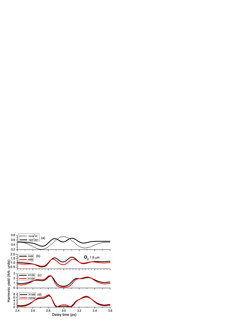
Figure 15: (Color online) HHG yield from O₂ for different harmonics as function of pump-probe delay time near quarter-revival. $\langle\sin^{2}(2\theta)\rangle$ and $\langle\cos^{2}(\theta)\rangle$ are also plotted for reference (a). Calculations are performed with a 1600-nm laser pulse with peak intensity of $2\times 10^{14}$ W/cm² and 20 fs duration.

In Fig. 15 we show a typical behavior of the HHG yield as function of delay time between pump and probe laser pulses for H49 and H69 in the lower plateau, H129 and H159 in the middle plateau, and H189 and H209 near the cutoff. The calculations were carried out with a 1600-nm laser pulse with peak intensity of $2\times 10^{14}$ W/cm² and 20 fs duration (FWHM). For the pump we use 800-nm pulse with $4\times 10^{13}$ W/cm² and 120 fs duration. We only focus on the results near the quarter-revival (near 3 ps), when the molecule can be most strongly aligned. This is in contrast to CO₂ where most strong alignment is achieved near 3/4-revival. The difference is caused by the different symmetries of the total electronic ground state wavefunctions, as discussed in Sec. II(F). Clearly the behaviors are quite different for these energy ranges. In the lower plateau, the HHG yield follows $\langle\sin^{2}(2\theta)\rangle$. This behavior is the same as for the case of 800-nm laser. In the middle plateau, the behavior starts to look similar to that of CO₂, which follows the inverted of $\langle\cos^{2}(\theta)\rangle$. This reflects the fact that the photoionization DCS peaks have shifted to larger angles for higher photon energy. Finally, for even higher harmonics an additional peak occurs right at the quarter-revival. This is also similar to the case of CO₂ near H31 for 800-nm, where the transition dipole goes through a minimum. Note that a quite high degree of alignment is needed in order to observe these additional peaks, which is not as pronounced as in CO₂ near 3/4-revival.

VI Summary and Outlook

In this paper we give detailed description of the quantitative rescattering theory (QRS) applied for high-order harmonic generation (HHG) by intense laser pulses. Although HHG has been described by the three-step model corkum in its many versions, including the Lewenstein model lewenstein , quantum orbits theory milosevic-review since the mid 1990’s, the calculated HHG spectra are known to be inaccurate, especially in the lower plateau region, as compared to accurate results from the TDSE. At the same time, numerical solution of the TDSE for molecules in intense laser pulses still remains a formidable challenge and has been carried out only for the simplest molecular system H${}_{2}^{+}$ so far. The QRS has been shown to provide a simple method for calculating accurate HHG spectra generated by atoms and molecules. The essence of the QRS is contained in Eq. (60) which states that harmonic dipole can be presented as a product of the returning electron wave packet and exact photo-recombination dipole for transition from a laser-free continuum state back to the initial bound state. The validity of the QRS has been carefully examined by checking against accurate results for both harmonic magnitude and phase from the solution of the TDSE for atomic targets within the single active electron approximation. For molecular targets, the QRS has been mostly tested for self-consistency in this paper. More careful tests have been reported earlier in Ref. H2+ for H${}_{2}^{+}$, for which accurate TDSE results are available. The results from the QRS for molecules are in very good agreement with available experimental data, whereas the SFA results are only qualitative at best.

Here are a number of the most important results of the QRS.

(i) The wave packet is largely independent of the target and therefore can be obtained from a reference atom, for which numerical solution of the TDSE can be carried out, if needed. It can also be calculated from the SFA. The shape of the wave packet depends on the laser parameters only, but its magnitude also depends on the target through the ionization probability for electron emission along laser polarization direction.

(ii) By using the factorization of HHG and the independence of the wave packet of the target structure, accurate photo-recombination transition dipole and phase can be retrieved from HHG experiments. This has been demonstrated for atomic targets, both theoretically toru ; atle08 and experimentally minemoto08 , and more recently for CO₂ atle09 .

(iii) Since the QRS is almost as simple as the SFA, it can be useful for realistic simulations of experiments, where macroscopic propagation needs to be carried out. For such simulations contributions from hundreds of intensities are needed. Existing macroscopic progagation simulations have rarely been done beyond the SFA model even for atomic targets. In the QRS the most time-consuming part is the calculation of the photoionizaion transition dipole. However, this needs to be done only once for each system, independently of laser parameters. The use of the QRS would significantly improve the SFA macroscopic results, but with the same computational effort as for the SFA.

(iv) Because of the inherent factorization, the QRS allows one to improve separately the quality of the wave packet and of the transition dipole. In particular, one can include many-electron effect in the photoionization process, which has been performed routinely in the atomic and molecular photoionization research.

The are several limitations of the QRS. Clearly, the method is not expected to work well in the multiphoton regime since QRS is based on the rescattering physics. Wave packets from the SFA becomes less accurate for lower plateau. We have seen that this has affected both harmonic yield and phase. This is probably due to the fact that the electron-core interaction has been neglected in the SFA during the electron propagation in the continuum. Remedy for this effect has been suggested by including some correction to the semi-classical action ivanov96 . We emphasize that the QRS so far only improves the last step of the three-step model by using exact photo-recombination transition dipole. Lastly we mention that similarity of the wave packets from different targets only holds for low to moderate intensities. Near saturation intensities, when depletion effect is large, the wave packets from targets with different ionization rates would be very different. Nevertheless, one can still use the wave packet from the SFA, provided the depletion is properly included.

The evidence presented in this work strongly supports that the QRS provides as a powerful method to obtain accurate HHG yield and phase from molecules under intense infrared laser pulses. As the technology of HHG generation improves, one can count on the retrieval of accurate photoionization cross section and phase from such measurement from aligned molecules. By using a pump beam to initiate a chemical reaction and a probe laser beam to generate high-order harmonics in a standard pump-probe scheme, the QRS would allow the retrieval of the transition dipole magnitude and phase over a broad range of photon energies, thus paving the way for extracting the structure information of the transient molecule, to achieve ultrafast chemical imaging with femtosecond temporal resolutions. In the meanwhile, with accurate single atom or single molecule induced dipole moments readily calculated, it is also possible to examine the effect of macroscopic propagation of the harmonics in the gaseous medium.

References

- (1) Spielmann C, Burnett NH, Sartania S, Koppitsch R, Schnurer M, Kan C, Lenzner M, Wobrauschek P, and Krausz F, Science 278, 661 664 (1997).
- (2) Z. Chang, A. Rundquist, H. Wang, M. M. Murnane, and Henry C. Kapteyn, Phys. Rev. Lett. 79, 2967 (1997).
- (3) F. Krausz and M. Ivanov, Rev. Mod. Phys. 81, 163 (2009).
- (4) I. Thomann, R. Lock, V. Sharma, E. Gagnon, S. T. Pratt, H. C. Kapteyn, M. M. Murnane, and W. Li, J. Phys. Chem. A 112, 9382 (2008).
- (5) M. Drescher, M. Hentschel, R. Kienberger, M. Uiberacker, V. Yakovlev, A. Scrinizi, T. Westerwalbesloh, U. Kleineberg, U. Heinzmann, and F. Krausz, Nature (London) 419, 803 (2002).
- (6) T. Sekikawa, A. Kosuge, T. Kanai, S. Watanabe, Nature (London) 432, 605 (2004).
- (7) G. Sansone et al., Science 314, 443 (2006).
- (8) R. Lopez-Martens et al., Phys. Rev. Lett. 94, 033001 (2005).
- (9) H. Stapelfeldt and T. Seideman, Rev. Mod. Phys. 75, 543 (2003).
- (10) J. Itatani, D. Zeidler, J. Levesque, M. Spanner, D. M. Villeneuve, and P. B. Corkum, Phys. Rev. Lett. 94, 123902 (2005).
- (11) J. Itatani, J. Levesque, D. Zeidler, H. Niikura, H. Pepen, J. C. Kiefer, P. B. Corkum, and D. M. Villeneuve, Nature 432, 867 (2004).
- (12) M. Lein, N. Hay, R. Velotta, J. P. Marangos, and P. L. Knight, Phys. Rev. Lett. 88, 183903 (2002).
- (13) M. Lein, P. P. Corso, J. P. Marangos, and P. L. Knight, Phys. Rev. A 67, 023819 (2004).
- (14) T. Kanai, S. Minemoto, and H. Sakai, Nature 435, 470 (2005).
- (15) C. Vozzi et al., Phys. Rev. Lett. 95, 153902 (2005).
- (16) X. Zhou, R. Lock, W. Li, N. Wagner, M. M. Murnane, and H. C. Kapteyn, Phys. Rev. Lett. 100, 073902 (2008).
- (17) N. Wagner, X. Zhou, R. Lock, W. Li, A. Wüest, M. Murnane, and H. C. Kapteyn, Phys. Rev. A 76, 061403 (2007).
- (18) W. Boutu et al., Nature Physics 4, 545 (2008).
- (19) T. Kanai, E. J. Takahashi, Y. Nabekawa, and K. Midorikawa, Phys. Rev. A 77, 041402 (2008).
- (20) P. B. Corkum, Phys. Rev. Lett. 71, 1994 (1993).
- (21) J. L. Krause, K. J. Schafer, and K. C. Kulander, Phys. Rev. Lett. 68, 3535 (1993).
- (22) M. Lewenstein, Ph. Balcou, M. Yu. Ivanov, A. L’Huillier, and P. B. Corkum, Phys. Rev. A 49, 2117 (1994).
- (23) M. Yu. Ivanov, T. Brabec, and N. Burnett, Phys. Rev. A 54, 742 (1996).
- (24) J. Z. Kaminski, A. Jaron, and F. Ehlotzky, Phys. Rev. A 53, 1756 (1996).
- (25) O. Smirnova, M. Spanner, and M. Ivanov, Phys. Rev. A 77, 033407 (2008).
- (26) G. L. Kamta and A. D. Bandrauk, Phys. Rev. A 71, 053407 (2005).
- (27) D. A. Telnov and S. I. Chu, Phys. Rev. A 76, 043412 (2007).
- (28) X. X. Zhou, X. M. Tong, Z. X. Zhao, and C. D. Lin, Phys. Rev. A 71, 061801(R) (2005).
- (29) X. X. Zhou, X. M. Tong, Z. X. Zhao, and C. D. Lin, Phys. Rev. A 72, 033412 (2005).
- (30) A. T. Le, X. M. Tong, and C. D Lin, Phys. Rev. A 73, 041402(R) (2006).
- (31) A. T. Le, X. M. Tong, and C. D Lin, J. Mod. Optics 54, 967 ( 2007).
- (32) J. P Marangos et al, J. Mod. Optics 53, 97 (2006).
- (33) S. Ramakrishna and T. Seideman, Phys. Rev. Lett. 99, 113901 (2007).
- (34) S. Odzak and D. B. Milosevic, Phys. Rev. A 79, 023414 (2009).
- (35) A. Abdurrouf and F. H. M. Faisal, Phys. Rev. A bf 79, 023405 (2009).
- (36) A. T. Le, T. Morishita, and C. D Lin, Phys. Rev. A 78, 023814 (2008).
- (37) A. T. Le, R. D. Picca, P.D. Fainstein, D. A. Telnov, M. Lein, and C.D. Lin, J. Phys. B 41, 081002 (2008).
- (38) T. Morishita, A. T. Le, Z. Chen, and C. D. Lin, Phys. Rev. Lett. 100, 013903 (2008).
- (39) Z. Chen, A. T. Le, T. Morishita, and C. D. Lin, J. Phys. B 42, 061001 (2009).
- (40) S. Micheau, Z. Chen, A. T. Le, J. Rauschenberger, M. F. Kling, and C. D. Lin, Phys. Rev. Lett. 102, 073001 (2009).
- (41) S. Micheau, Z. Chen, T. Morishita, A. T. Le, and C. D. Lin, J. Phys. B 42, 065402 (2009).
- (42) Z. Chen, A. T. Le, T. Morishita, and C. D. Lin, Phys. Rev. A 79, 033409 (2009).
- (43) Z. Chen, T. Morishita, A. T. Le, and C. D. Lin, Phys. Rev. A 76, 043402 (2007).
- (44) S. Micheau, Z. Chen, A. T. Le, and C. D. Lin, Phys. Rev. A 79, 013417 (2009).
- (45) R. R. Lucchese, G. Raseev, and V. McKoy, Phys. Rev. A 25, 2572 (1982).
- (46) R. E. Stratmann and R. R. Lucchese, J. Chem. Phys. 102, 8493 (1995).
- (47) C. Jin, A. T. Le, and C. D. Lin, in preparation.
- (48) Z. Chen, T. Morishita, A. T. Le, M. Wickenhauser, X. M. Tong, and C. D. Lin, Phys. Rev. A 74, 053405 (2006).
- (49) T. Morishita, Z. Chen, S. Watanabe, and C. D. Lin, Phys. Rev. A 75, 023407 (2007).
- (50) X. M. Tong and C. D. Lin, J. Phys. B 38, 2593 (2005).
- (51) J. C. Light, I. P. Hamilton, and J. V. Lill, J. Chem. Phys. 82, 1400 (1985).
- (52) X. M. Tong and S. I. Chu, Chem. Phys. 217, 119 (1997).
- (53) K. Burnett, V. C. Reed, J. Cooper, and P. L. Knight, Phys. Rev. A 45, 3347 (1992).
- (54) M. W. Schmidt et al., J. Comput. Chem. 14, 1347 (1993).
- (55) M. J. Frisch et al., GAUSSIAN 03, revision C.02, (Gaussian Inc., Pittsburgh, PA, 2003).
- (56) A. F. Starace, Theory of atomic photoionization, p. 14, Springer Verlag, Berlin (1982).
- (57) L. D. Landau and E. M. Lifshitz, Quantum mechanics: Non relativistic theory, Pergamon Press 1965, p. 553.
- (58) H. A. Bethe and E. E. Salpeter, Quantum mechanics of one- and two-electron atoms, Springer-Verlag 1957, p. 253.
- (59) J. W. Cooper, Phys. Rev. 128, 681 (1962).
- (60) U. Fano and J. W Cooper, Rev. Mod. Phys. 40, 441 (1968).
- (61) H.-J. Werner, P. J. Knowles, R. Lindh, M. Schütz and others, MOLPRO, version 2002.6, a package of ab initio programs (Birmingham, UK, 2003).
- (62) R. E. Stratmann, R. W. Zurales, and R. R. Lucchese, J. Chem. Phys. 104, 8989 (1996).
- (63) B. Basden and R. R. Lucchese, Phys. Rev. A 37, 89 (1988).
- (64) G. Bandarage and R. R. Lucchese, Phys. Rev. A 47, 1989 (1993).
- (65) A. P. P. Natalense and R. R. Lucchese, J. Chem. Phys. 111, 5344 (1999).
- (66) S. Tonzani, Comput. Phys. Comm. 176, 146 (2007).
- (67) X. M. Tong, Z. X. Zhao, and C. D. Lin, Phys. Rev. A 66, 033402 (2002).
- (68) T. K. Kjeldsen and L. B. Madsen, Phys. Rev. A 71, 023411 (2005).
- (69) J. Muth-Böhm, A. Becker, and F. H. Faisal, Phys. Rev. Lett. 85, 2280 (2000).
- (70) V. H. Le, N. T. Nguyen, C. Jin, A. T. Le, and C. D. Lin, J. Phys. B 41, 085603 (2008).
- (71) D. Pavicic, K. F. Lee, D. M. Rayner, P. B. Corkum, and D. M. Villeneuve, Phys. Rev. Lett. 98, 243001 (2007).
- (72) J. Ortigoso, M. Rodriguez, M. Gupta, and B. Friedrich, J. Chem. Phys. 110, 3870 (1999).
- (73) G. Herzberg, Molecular Spectra and Molecular Structure, I. Spectra of Diatomic Molecules (Van Nostrand Reinhold, New York, 1950), Chap. III(f).
- (74) J. O. Hirschfelder, C. F. Curtiss, and R. B. Bird, Molecular Theory of Gases and Liquids (Wiley, New York, 1954).
- (75) P. J. Linstrom and W. G. Mallard, Eds., NIST Chemistry WebBook, NIST Standard Reference Database Number 69, National Institute of Standards and Technology, Gaithersburg MD, 20899, http://webbook.nist.gov.
- (76) M. Lein et al., J. Mod. Optics 52, 465 (2005).
- (77) J. Levesque, D. Zeidler, J. P. Marangos, P. B. Corkum, and D. M. Villeneuve, Phys. Rev. Lett. 98, 183903 (2007).
- (78) V. H. Le, A. T. Le, R. H. Xie, and C. D. Lin, Phys. Rev. A. 76, 013414 (2007).
- (79) T. K. Kjeldsen, L. A. Nikolopoulos, and L. B. Madsen, Phys. Rev. A 75, 063427 (2007).
- (80) Y.-M. Lee, J.-S. Wu, T.-F. Jiang, and Y.-S. Chen, Phys. Rev. A 77, 013414 (2008).
- (81) A. T. Le, R. R. Lucchese, M. T. Lee, and C. D. Lin, submitted to Phys. Rev. Lett. ; arXiv:0901.1311v1.
- (82) A. T. Le and C. D. Lin, unpublished.
- (83) M. V. Frolov, N. L. Manakov, T. S. Sarantseva, and A. F. Starace, J. Phys. B 42, 035601 (2009).
- (84) H. G. Muller, Phys. Rev. A 60, 1341 (1999).
- (85) M. J. Nandor, M. A. Walker, L. D. Van Woerkom, and H. G. Muller, Phys. Rev. A 60, R1771 (1999).
- (86) S. Minemoto, T. Umegaki, Y. Oguchi, T. Morishita, A. T. Le, S. Watanabe, and H. Sakai, Phys. Rev. A 78, 061402(R) (2008).
- (87) H. J. Wörner, H. Niikura, J. B. Bertrand, P. B. Corkum, and D. M. Villeneuve, Phys. Rev. Lett. 102, 103901 (2009).
- (88) C. D. Lin, Phys. Rev. A 9, 181 (1974).
- (89) M. Ya. Amusia, N. A. Cherepkov, and L. V. Chernysheva, Sov. Phys. JETP 33, 90 (1971).
- (90) Y. Mairesse, J. Levesque, N. Dudovich, P. B. Corkum, and D. M. Villeneuve, J. Mod. Optics 55, 2591 (2008).
- (91) K. Miyazaki, M. Kaku, G. Miyaji, A. Abdurrouf, and F. H. M. Faisal, Phys. Rev. Lett. 95, 243903 (2005).
- (92) C. B. Madsen and L. B. Madsen, Phys. Rev. A 74, 023403 (2006).
- (93) X. Zhou, N. Wagner, M. Murnane, H. Kapteyn, private communication.
- (94) O. Smirnova, S. Patchkovskii, Y. Mairesse, N. Dudovich, D. Villeneuve, P. Corkum, and M. Yu. Ivanov, Phys. Rev. Lett. 102 063601 (2009).
- (95) P. Liu, P. Yu, Z. Zeng, H. Xiong, X. Ge, R. Li, and Z. Xu, Phys. Rev. A 78, 015802 (2008).
- (96) A. S. Alnaser, C. M. Maharjan, X. M. Tong, B. Ulrich, P. Ranitovic, B. Shan, Z. Chang, C. D. Lin, C. L. Cocke, and I. V. Litvinyuk, Phys. Rev. A 71, 031403(R), (2005).
- (97) B. Zimmermann, M. Lein, and J. M. Rost, Phys. Rev. A 71, 033401 (2005).
- (98) E. J. Takahashi, T. Kanai, K. L. Ishikawa, Y. Nabekawa, and K. Midorikawa, Phys. Rev. Lett. 101, 253901 (2008).
- (99) D. B. Milosevic, G. G. Paulus, D. Bauer, and W. Becker, J. Phys. B 39, R203 (2006).