On the Structure of Supersymmetric Sums in Multi-Loop Unitarity Cuts

Abstract

In this paper we describe algebraic and diagrammatic methods, related to the MHV generating function method, for evaluating and exposing the structure of supersymmetric sums over the states crossing generalized unitarity cuts of multi-loop amplitudes in four dimensions. We focus mainly on cuts of maximally supersymmetric Yang-Mills amplitudes. We provide various concrete examples, some of which are directly relevant for the calculation of four-loop amplitudes. Additionally, we discuss some cases with less than maximal supersymmetry. The results of these constructions carry over to generalized cuts of multi-loop supergravity amplitudes through use of the Kawai-Lewellen-Tye relations between gravity and gauge-theory tree amplitudes.

I Introduction

Multi-loop scattering amplitudes in maximally supersymmetric gauge and gravity theories have received considerable attention in recent years for their roles BCDKS ; ABDK ; BDS ; AM in helping to confirm and utilize Maldacena’s AdS/CFT correspondence Maldacena and in probing the ultraviolet structure of supergravity theories Finite ; GravityThree ; CompactThree .

In particular, multi-loop calculations offer important insight into the possibility that planar ${{\cal N}=4}$ super-Yang-Mills scattering amplitudes can be resummed to all loop orders ABDK ; BDS ; AM . In ref. ABDK a loop iterative structure was suggested, leading to the detailed BDS conjecture BDS for planar maximally-helicity-violating (MHV) amplitudes to all loop orders. Alday and Maldacena realized that certain planar scattering amplitudes at strong coupling may be evaluated as the regularized area of minimal surfaces in AdS${}_{5}\times$S⁵ with special boundary conditions, and for four-point amplitudes they confirmed the BDS prediction. Direct evidence suggests that the all-order resummation holds as well for five-point amplitudes TwoLoopFive . The structure of the four- and five-point planar amplitudes is now understood as a consequence DHKS of a new symmetry dubbed “dual conformal invariance” DualConformal ; BCDKS ; FiveLoop , with further generalizations at tree level DrummondYangian and at infinite ’t Hooft coupling BerkovitsMaldacena . However, beyond five points, the BDS conjecture requires modification AM2 ; Lipatov ; TwoLoopSixPt . High-loop calculations in ${{\cal N}=4}$ super-Yang-Mills theory should also play a useful role in clarifying the structure of subleading color contributions to the soft anomalous dimension matrix of gauge theories SoftMatrixPapers , once the evaluation of the required nonplanar integrals becomes feasible at three loops and beyond.

In a parallel development, studies of multi-loop amplitudes in ${{\cal N}=8}$ supergravity  CremmerJuliaScherk have suggested that this theory may be ultraviolet finite in four dimensions Finite ; GravityThree ; CompactThree , challenging the conventional understanding of the ultraviolet properties of gravity theories. For a class of terms accessible by isolating one-loop subamplitudes via generalized unitarity GeneralizedUnitarity ; TwoLoopSplit ; BCFGeneralized , the one-loop “no-triangle” property (OneloopMHVGravity ; NoTriangle ; UnexpectedCancel ; AHCKGravity ) shows that at least a subset of these cancellations persist to all loop orders Finite . The direct calculation of the three-loop four-point amplitude of ${{\cal N}=8}$ supergravity exposes cancellations beyond those needed for ultraviolet finiteness in $D=4$ in all terms contributing to the amplitude GravityThree ; CompactThree . Interestingly, $M$ theory and string theory have also been used to argue either for the finiteness of ${{\cal N}=8}$ supergravity DualityArguments , or that divergences are delayed through at least nine loops Berkovits ; GreenII , though issues with decoupling towers of massive states GOS may alter these conclusions. A recent direct field theory study proposes that a divergence may first appear at the five loop order in $D=4$, though this can be softer if additional unaccounted symmetries are present HoweStelleRecent . If a perturbatively ultraviolet-finite point-like theory of quantum gravity could be constructed, the underlying mechanism responsible for the required cancellations is expected to have a fundamental impact on our understanding of gravity.

The recent studies of multi-loop amplitudes rely on the modern unitarity method UnitarityMethod ; Fusing as well as various refinements GeneralizedUnitarity ; TwoLoopSplit ; BCFGeneralized ; FiveLoop ; FreddyMaximal . In this approach multi-loop amplitudes are constructed directly from on-shell tree amplitudes. This formalism takes advantage of the fact that tree-level amplitudes are much simpler than individual Feynman diagrams, as well as makes use of various properties that hold only on shell. In particular, it provides a means of using an on-shell superspace—which is much simpler than its off-shell cousins—in the construction of loops amplitudes.

Summing over the physical states of propagating fields is one essential ingredient in higher-loop calculations. In particular, the modern unitarity method uses these sums over physical on-shell states in the reconstruction of any loop amplitude in terms of covariant integrals with internal off-shell lines. In supersymmetric theories the on-shell states can be organized in supermultiplets dictated by the supersymmetry. Systematic approaches to evaluate such supersymmetric sums—or supersums—have recently been discussed in refs. FreedmanGenerating ; FreedmanUnitarity ; KorchemskyOneLoop ; AHCKGravity . As the calculations reach to ever higher loop orders these sums become more intricate. It is therefore helpful to expose their structure and simplify their evaluation as much as possible. In this paper we describe algebraic and diagrammatic methods which are helpful in this direction. These methods are the ones used in the course of computing and confirming the four-loop four-point amplitude of maximally supersymmetric Yang-Mills theory, including nonplanar contributions. The main aspects of the construction of this amplitude, as well as the explicit results, will be presented elsewhere FourLoopNonPlanar . (The planar contributions are given in ref. BCDKS .)

Supersymmetric cancellations were extensively discussed at one and two loops in refs. UnitarityMethod ; Fusing ; BRY ; BDDPR using a component formalism that exploits supersymmetry Ward identities SWI . These supersums were relatively simple, making it straightforward to sum over the contributions from the supermultiplet in components. The recent calculations of more complicated amplitudes in refs. TwoLoopFive ; FiveLoop ; GravityThree ; TwoLoopSixPt ; LeadingApplications ; CompactThree , are performed in ways obscuring the systematics of the supersums. For example, as explained in ref. FiveLoop , it is possible to avoid evaluating (sometimes complicated) supersums in maximally supersymmetric Yang-Mills theory via the method of maximal cuts, where kinematics can be chosen to restrict scalars and fermions to a small (even zero) number of loops. Remarkably, this trick is sufficient to construct ansätze for ${{\cal N}=4}$ super-Yang-Mills amplitudes. However, any such ansatz needs to be confirmed by more direct evaluations incorporating all particles in the supermultiplet, to ensure that no terms are dropped. It is therefore necessary to compare the cuts of the ansatz with the cuts of the amplitude for more general kinematic configurations, allowing all states to cross the cuts. The calculation of supersums is a crucial ingredient in carrying out this comparison. Moreover, formal studies of the ultraviolet behavior of multi-loop amplitudes of supersymmetric theories, in particular of ${{\cal N}=8}$ supergravity, are substantially aided by a formalism that exposes the supersymmetric cancellations.

Nair’s original construction of an on-shell superspace Nair captured only MHV tree amplitudes in ${{\cal N}=4}$ super-Yang-Mills theory; more recent developments extend this to any helicity and particle configuration. The approach of GGK ; FreedmanGenerating ; FreedmanUnitarity ; FreedmanProof makes use of the MHV vertex expansion CSW to extend this on-shell superspace to general amplitudes. Another strategy, discussed in refs. AHCKGravity ; RecentOnShellSuperSpace , makes use of the Britto, Cachazo, Feng, and Witten (BCFW) on-shell recursion BCFW to extend the MHV on-shell superspace to general helicity configurations. A new key ingredient of this approach is a shift involving anti-commuting parameters which may be thought of as the supersymmetric extension of the BCFW shift of space-time momenta. A recent paper uses shifts of anti-commuting parameters to construct a new super-MHV expansion Kiermaier , which we do not use here. With the unitarity method UnitarityMethod ; Fusing ; BRY ; BDDPR , superspace expressions for tree amplitudes can be extended to loop level. One-loop constructions along these lines were discussed in refs. FreedmanGenerating ; KorchemskyOneLoop ; AHCKGravity , while various examples of supersums in higher-loop cuts, including four-loop ones, have already been presented in ref. FreedmanUnitarity .

The MHV vertex expansion suggests an inductive structure for supersymmetric cancellations. Once these cancellations are exposed and understood for cuts with only MHV or $\overline{\hbox{MHV}}$ tree amplitudes, more general cuts with non-MHV amplitudes follow rather simply FreedmanUnitarity . Indeed, the prescription for evaluating these more general cuts involves summing over MHV contributions with shifts of certain on-shell intermediate momenta.

To evaluate the supersymmetric sums that appear in unitarity cuts we introduce complementary algebraic and diagrammatic approaches. The algebraic approach has the advantage of exposing supersymmetric cancellations, in many cases leading to simple expressions. It is a natural approach for formal proofs. In particular, it allows us to systematically expose supersymmetric cancellations—within the context of the unitarity method—sufficient for exhibiting the well known Mandelstam all-loop ultraviolet finiteness of ${{\cal N}=4}$ super-Yang-Mills theory. The diagrammatic approach gives us a means of pictorially tracking contributions, allowing us to write down the answer directly by drawing a set of simple diagrams. It also leads to a simple algorithms for writing down the results for any cut by sweeping over all possible helicity labels. Since it tracks contributions of individual states, it can be easily applied to a variety of cases with fewer supersymmetries. To illustrate these techniques we present various examples, including those relevant for evaluating the four-loop four-point amplitude of ${{\cal N}=4}$ super-Yang-Mills theory FourLoopNonPlanar . We will also show that these techniques are not restricted to four-point amplitudes by discussing some higher-point examples.

One potential difficulty with any four-dimensional approach is that unitarity cuts are properly evaluated in $D$ dimensions DDimUnitarity ; SelfDual , since they rely on a form of dimensional regularization FDH related to dimensional reduction Siegel . Moreover, a frequent goal in multi-loop calculations is the determination of the critical dimension in which ultraviolet divergences first appear. Consequently, such calculations often need to be valid away from four dimensions. This requirement complicates the analysis significantly, because powerful four-dimensional helicity methods SpinorHelicity can no longer be used. Any ansatz for an amplitude obtained with intrinsically four-dimensional methods, such as the ones of the present paper, needs to be confirmed through $D$-dimensional calculation. Nevertheless, the $D=4$ analysis offers crucial guidance for the construction of $D$-dimensional amplitudes. Additionally, $D=4$ methods appear to capture the complete result for four-point ${{\cal N}=4}$ super-Yang-Mills amplitudes with fewer than five loops BRY ; BDDPR ; BCDKS ; GravityThree .

While difficulties appear to arise with extending the MHV diagram expansion to general ${{\cal N}=8}$ supergravity tree amplitudes FreedmanGenerating , they will not concern us here. Instead we rely on the Kawai-Lewellen-Tye (KLT) relations KLT ; GeneralKLT , or their reorganization in terms of diagram-by-diagram relations TreeJacobi , to obtain the sums over supermultiplets in ${{\cal N}=8}$ supergravity cuts directly from the cuts of corresponding ${{\cal N}=4}$ super-Yang-Mills theory amplitudes.

This paper is organized as follows. In section II we review on-shell superspace at tree level and introduce $SU(4)$ $R$-symmetry index diagrams. In section III we review the modern unitarity method and present the general structure of supercuts. In section IV we explain how the supersums can be evaluated in terms of the determinant of the matrix of coefficients of a system of linear equations. This section also contains various examples of cuts of ${{\cal N}=4}$ super-Yang-Mills, including those of a five-point amplitude at four loops. Section V describes supersums in terms of $R$-symmetry index diagrams, providing pictorial means for tracking different contributions. As discussed in section VI, these diagrams allow us to relate the cuts of amplitudes with fewer supersymmetries to maximally supersymmetric ones. They also allow us construct a simple algorithm for obtaining all contributions to cuts from purely gluonic ones. Various three and four-loop examples are presented in sections V and VI. In section VII we outline the use of the KLT relations to carry over the results for the sum over states in cuts of ${{\cal N}=4}$ super-Yang-Mills amplitudes to the corresponding ones of ${{\cal N}=8}$ supergravity theory. Our conclusions are presented in section VIII.

II On-shell superspace at tree level

On-shell superspaces are useful tools for probing the properties of supersymmetric field theories, providing information on their structure without any complications due to unphysical degrees of freedom. Here we review the construction of an on-shell superspace for ${{\cal N}=4}$ super-Yang-Mills amplitudes. In its original form, devised by Nair Nair , it described maximally helicity violating (MHV) gluon amplitudes and their supersymmetric partners. While we will depart at times from Nair’s original construction, the main features will persist. This same superspace also captures general amplitudes. Indeed, there currently exists two methods for constructing general amplitudes from MHV amplitudes: the MHV vertex construction of Cachazo, Svrček and Witten CSW and the on-shell recursion relation of Britto, Cachazo, Feng and Witten (BCFW) BCFW . The supersymmetric extension of the former approach has been given in refs. GGK ; FreedmanGenerating ; FreedmanUnitarity ; FreedmanProof , while that of the latter approach in refs. AHCKGravity ; RecentOnShellSuperSpace .

To evaluate the supersum in unitarity cuts we will use an approach based on MHV vertices, along the lines taken by Bianchi, Elvang, Freedman and Kiermaier FreedmanGenerating ; FreedmanUnitarity . We will find that supersums involving only MHV and/or $\overline{\hbox{MHV}}$ tree amplitudes have a surprisingly simple structure. We will also show how the MHV vertex construction allows us to immediately carry over this simplicity, with only minor modifications, to more general cuts involving arbitrary non-MHV tree amplitudes.

The on-shell superspace of the type we will review here generalizes easily to MHV and $\overline{\hbox{MHV}}$ amplitudes in ${{\cal N}=8}$ supergravity. Difficulties however, appear with the MHV vertex construction of non-MHV gravity tree amplitudes because the on-shell recursions used to obtain the expansion GravityMHV can fail to capture all contributions FreedmanGenerating . Such amplitudes may nevertheless be found without difficulty through supersymmetric extensions AHCKGravity of the on-shell BCFW recursion relations BCFW ; CachazoLargez , which do carry over to ${{\cal N}=8}$ supergravity. However, at present BDDPR ; GravityThree ; CompactThree we find it advantageous to use the KLT tree-level relations KLT ; GeneralKLT or the recently discovered diagram-by-diagram relations TreeJacobi , to obtain ${{\cal N}=8}$ supergravity unitarity cuts directly from those of ${{\cal N}=4}$ super-Yang-Mills theory.

II.1 MHV amplitudes in ${{\cal N}=4}$ super-Yang-Mills

The vector multiplet of the ${{\cal N}=4}$ supersymmetry algebra consists of one gluon, four gluinos and three complex scalars, all in the adjoint representation of the gauge group, which here we take to be $SU(N_{c})$. With all states in the adjoint representation, any complete tree-level amplitude can be decomposed as

$$\mathbb{A}^{\rm tree}_{n}(1,2,3,\ldots,n)=g^{n-2}\sum_{{\cal P}(2,3,\ldots,n)}{\rm Tr}[T^{a_{1}}T^{a_{2}}T^{a_{3}}\cdots T^{a_{n}}]\,A^{\rm tree}_{n}(1,2,3,\ldots,n),$$ (1)

where $A_{n}^{\rm tree}$ are tree-level color-ordered $n$-leg partial amplitudes. The $T^{a_{i}}$’s are generators of the gauge group and encode the color of each external leg $1,2,3\ldots n$, with color group indices $a_{i}$. The sum runs over all noncyclic permutations of legs, which is equivalent to all permutations keeping one leg fixed (here leg $1$). Helicities and polarizations are suppressed. We use the all outgoing convention for the momenta to define the amplitudes.

All states transform in antisymmetric tensor representations of the $SU(4)$ $R$-symmetry group such that states with opposite helicities are in conjugate representations. The $R$-symmetry and helicity quantum numbers uniquely specify all on-shell states:

$$g_{+}\,,\hskip 42.67912ptf_{+}^{a}\,,\hskip 42.67912pts^{ab},\hskip 42.67912ptf^{abc}_{-}\,,\hskip 42.67912ptg_{-}^{abcd}\,,$$ (2)

where $g_{\pm}$ and $f_{\pm}$ are, respectively, the positive and negative helicity gluons and gluinos while $s^{ab}$ are scalars. (The scalars are complex-valued and obey a self-duality condition which will not be relevant here.) These fields are completely antisymmetric in their displayed $R$-symmetry indices—denoted by $a,b,c,d$—which transform in the fundamental representation of $SU(4)$, giving a total of 16 states in the on-shell multiplet.

Alternatively, we can use the dual assignment obtained by lowering the indices with a properly normalized Levi-Civita symbol $\varepsilon_{abcd}$, giving the fields,

$$g^{+}_{abcd}\,,\hskip 42.67912ptf^{+}_{abc}\,,\hskip 42.67912pts_{ab},\hskip 42.67912ptf^{-}_{a}\,,\hskip 42.67912ptg^{-}\,.$$ (3)

We will use both representations to describe the amplitudes of ${{\cal N}=4}$ super-Yang-Mills. For MHV amplitudes we will mainly use the states with upper indices in eq. (2) whereas for $\overline{\hbox{MHV}}$ we will use mainly the states with lower indices in eq. (3). This is a matter of convenience, and the two sets of states may be interchanged, as we will briefly discuss later in this section.

We begin by discussing the MHV amplitudes, which we define as an amplitude with a total of eight (2 $\times$ 4 distinct) upper $SU(4)$ indices. (In order to respect $SU(4)$ invariance, amplitudes of the fields in eq. (2) must always come with $4m$ upper indices, where $m$ is an integer. Furthermore amplitudes with four or zero indices vanish as they are related by supersymmetry to vanishing SWI amplitudes.) Some simple examples of MHV amplitudes, which we will use in section II.3, are,

$${\rm(a)}:\;\;A_{4}^{\rm tree}(1^{-}_{g^{abcd}},2^{-}_{g^{abcd}},3^{+}_{g},4^{+}_{g})=i{\left\langle 1\,2\right\rangle^{4}\over\left\langle 1\,2\right\rangle\left\langle 2\,3\right\rangle\left\langle 3\,4\right\rangle\left\langle 4\,1\right\rangle}\,,$$

$${\rm(b)}:\;\;A_{4}^{\rm tree}(1^{-}_{g^{abcd}},2^{-}_{f^{abc}},3^{+}_{f^{d}},4^{+}_{g})=i{\left\langle 1\,2\right\rangle^{3}\left\langle 1\,3\right\rangle\over\left\langle 1\,2\right\rangle\left\langle 2\,3\right\rangle\left\langle 3\,4\right\rangle\left\langle 4\,1\right\rangle}\,,$$

$${\rm(c)}:\;\;A_{4}^{\rm tree}(1^{-}_{f^{abc}},2^{-}_{f^{abd}},3_{s^{cd}},4^{+}_{g})=i{\left\langle 1\,2\right\rangle^{2}\left\langle 1\,3\right\rangle\left\langle 2\,3\right\rangle\over\left\langle 1\,2\right\rangle\left\langle 2\,3\right\rangle\left\langle 3\,4\right\rangle\left\langle 4\,1\right\rangle}\,,$$ (4)

where $a,b,c,d$ are four distinct fundamental $SU(4)$ indices. The overall phases of these amplitudes depend on conventions. We will fix this ambiguity by demanding that the phases be consistent with the supersymmetry algebra, which is automatically enforced when using superspace. The amplitudes are written in terms of the familiar holomorphic and antiholomorphic spinor products,

$$\left\langle i\,j\right\rangle = \langle i|j\rangle=\bar{u}_{-}(p_{i})u_{+}(p_{j})=\varepsilon_{\alpha\beta}\lambda_{i}^{\alpha}\lambda_{j}^{\beta}\,,$$

$$\left[i\,j\right] = [i|j]=\bar{u}_{+}(p_{i})u_{-}(p_{j})=\varepsilon_{\dot{\alpha}\dot{\beta}}{\tilde{\lambda}}_{i}^{\dot{\alpha}}{\tilde{\lambda}}_{j}^{\dot{\beta}}\,,$$ (5)

where the $\lambda_{i}^{\alpha}$ and ${\tilde{\lambda}}_{i}^{\dot{\alpha}}$ are commuting spinors which may be identified with the positive and negative chirality solutions $|i\rangle=u_{+}(p_{i})$ and $|i]=u_{-}(p_{i})$ of the massless Dirac equation and the spinor indices are implicitly summed over. These products are antisymmetric, $\left\langle i\,j\right\rangle=-\left\langle j\,i\right\rangle$, $\left[i\,j\right]=-\left[j\,i\right]$.

Momenta are related to these spinors via

$$p_{i}^{\mu}\sigma_{\mu}^{\alpha{\dot{\alpha}}}=\lambda_{i}^{\alpha}{\tilde{\lambda}}_{i}^{{\dot{\alpha}}}\,\hskip 14.22636pt{\rm or}\hskip 14.22636ptp_{i}^{\mu}\sigma_{\mu}=|i\rangle[i|\,,$$ (6)

and similar formulæ hold for the expression of $p_{i}^{\mu}{\overline{\sigma}}_{\,\mu}$. We will often write simply $p_{i}=|i\rangle[i|$ or sometimes $p=|p\rangle[p|$. The proper contractions of momenta $p_{i}$ with spinorial objects will be implicitly assumed in the remainder of the paper. Typically, we will denote external momenta by $k_{i}$ and loop momenta by $l_{i}$.

A subtlety we must deal with is a slight inconsistency in the standard spinor helicity formalism for massless particles when a state crosses a cut. In a given cut we will always have the situation that on one side of a cut line the momentum is outgoing, but on the other side it is incoming. Thus across a cut we encounter expressions such as $|$$-i\rangle[i|$, which is not properly defined in our all-outgoing conventions and can lead to incorrect phases. This is because the spinor $|$$-i\rangle$ carries momentum $-p_{i}$, and thus it has an energy component of opposite sign to that carried by the spinor $[i|$. This problem is due to the fact that the spinor helicity formalism does not distinguish between particle and antiparticle spinors, as has been discussed and corrected in refs. SignSubtlety for the MHV vertex expansion, and for BCFW recursion relations with fermions. To deal with this, we use the analytic continuation rule that the change of of sign of the momentum is realized by the change in sign of the holomorphic spinor FreedmanUnitarity ,

$$p_{i}\mapsto-p_{i}~{}~{}~{} \leftrightarrow ~{}~{}~{}\lambda_{i}^{\alpha}\mapsto-\lambda_{i}^{\alpha}\,,~{}~{}~{}~{}~{}~{}{\tilde{\lambda}}_{i}^{\dot{\alpha}}\mapsto{\tilde{\lambda}}_{i}^{\dot{\alpha}}\,,$$

$$\leftrightarrow ~{}~{}|-i\rangle\mapsto-|i\rangle\,,~{}~{}~{}~{}|-i]\mapsto|i]\,.$$ (7)

II.2 The MHV Superspace

The supersymmetry relations between the different MHV amplitudes may be encoded in an on-shell superspace, which conveniently packages all amplitudes into a single object—the generating function or superamplitude. Each term in the superamplitude corresponds to a regular component scattering amplitude. Depending upon the detailed formulation of the superspace, scattering amplitudes of gluons, fermions and scalars are then formally extracted either by the application of Grassmann-valued derivatives FreedmanUnitarity , or, equivalently, by multiplying with the appropriate wave functions and integrating over all Grassmann variables Nair ; WittenTopologicalString . Effectively, these operations amount to selecting the component amplitude with the desired external states.

The MHV generating function (or superamplitude) is defined as,

$${\cal A}^{\rm MHV}_{n}(1,2,\ldots,n)\equiv\frac{i}{\prod_{j=1}^{n}\langle j~{}(j+1)\rangle}\,\delta^{(8)}\Bigl{(}\sum_{j=1}^{n}\lambda_{j}^{\alpha}\eta_{j}^{a}\Bigr{)}\,,$$ (8)

where the leg label $n+1$ is identified with the leg label $1$, and $\eta_{j}^{a}$ are $4n$ Grassmann odd variables labeled by leg $j$ and $SU(4)$ $R$-symmetry index $a$. As indicated by the cyclic denominator, this amplitude is color ordered (i.e., it is the kinematic coefficient of a particular color trace in eq. (1)), even though the numerator possesses full crossing symmetry having encoded all possible MHV helicity and particle assignments. We suppress the delta-function factor $(2\pi)^{4}\delta^{(4)}(\sum_{i}p_{i})=(2\pi)^{4}\delta^{(4)}(\sum_{i}\lambda_{i}{\tilde{\lambda}}_{i})$ responsible for enforcing the overall momentum conservation.

The eightfold Grassmann delta function in (8) is a product of pairs of delta functions, each pair being associated with one of the possible values of the $SU(4)$ $R$-symmetry index:

$$\delta^{(8)}\Bigl{(}\sum_{i=1}^{n}\lambda_{i}^{\alpha}\eta_{i}^{a}\Bigr{)}=\prod_{a=1}^{4}\delta^{(2)}\Bigl{(}\sum_{i=1}^{n}\lambda_{i}^{\alpha}\eta_{i}^{a}\Bigr{)}\,.$$ (9)

This expression can be further expanded,

$$\delta^{(8)}\Bigl{(}\sum_{i=1}^{n}\lambda_{i}^{\alpha}\eta_{i}^{a}\Bigr{)}=\prod_{a=1}^{4}\sum_{i<j}^{n}\left\langle i\,j\right\rangle\eta_{i}^{a}\eta_{j}^{a}\,,$$ (10)

using the usual property of Grassmann delta functions that $\delta(\eta)=\eta$. Each monomial in $\eta$ in the superamplitude corresponds to a different MHV amplitude. In this form it is clear that all terms indeed have eight upper $SU(4)$ indices, as expected for an MHV amplitude.

Similarly, one may define an on-shell $\overline{\hbox{MHV}}$ superspace, whose Grassmann parameters are $\widetilde{\eta}$, in which the $\overline{\hbox{MHV}}$ superamplitude takes a form analogous to (8):

$${\cal A}_{n}^{\rm\overline{MHV}}(1,2,\ldots,n) \equiv \frac{i(-1)^{n}}{\prod_{j=1}^{n}[j~{}(j+1)]}\;\delta^{(8)}\Bigl{(}\sum_{j=1}^{n}\tilde{\lambda}_{j}^{\dot{\alpha}}\widetilde{\eta}_{ja}\Bigr{)}$$ (11)

$$= \frac{i(-1)^{n}}{\prod_{j=1}^{n}[j~{}(j+1)]}\,\prod_{a=1}^{4}\sum_{i<j}^{n}\left[i\,j\right]\widetilde{\eta}_{ia}\widetilde{\eta}_{ja}\,.$$

The $SU(4)$ indices are now lowered, which implies that the component $\overline{\hbox{MHV}}$ amplitudes are built from the external states in (3) with a total of eight lower indices.

We note that the arguments of the MHV delta functions are the super-momenta $Q^{a}$, and for $\overline{\hbox{MHV}}$ are similarly the conjugate super-momenta $\widetilde{Q}_{a}$,

$$Q^{\alpha a}=\sum_{i}\lambda^{\alpha}_{i}\eta^{a}_{i}\,,~{}~{}~{}~{}~{}~{}~{}~{}\widetilde{Q}^{\dot{\alpha}}_{a}=\sum_{i}{\tilde{\lambda}}^{\dot{\alpha}}_{i}\widetilde{\eta}_{ia}\,,$$ (12)

where the index $i$ runs over all the external legs of the amplitude. Thus the purpose of the delta functions is to enforce super-momentum conservation constraint in the respective superspaces. For later purposes we define the individual super-momenta of the external legs,

$$q^{a}_{i}=|i\rangle\eta_{i}^{a}\,,~{}~{}~{}~{}~{}~{}~{}~{}\tilde{q}_{ia}=\widetilde{\eta}_{ia}[i|\,.$$ (13)

The two superspaces can be related. Following ref. FreedmanUnitarity we can rewrite the $\overline{\hbox{MHV}}$ superamplitudes in the MHV superspace (or $\eta$-superspace) via a Grassmann Fourier transform. For this purpose we define FreedmanUnitarity the operator,

$$\widehat{F}\bullet\equiv\int\Bigl{[}\prod_{i,a}d\widetilde{\eta}_{ia}\Bigr{]}\exp\Bigl{(}\sum_{b,j}\eta_{j}^{b}~{}\widetilde{\eta}_{jb}\Bigl{)}\,\bullet~{}~{},$$ (14)

which realizes this Fourier transform. Then, following FreedmanUnitarity , the $\overline{\hbox{MHV}}$ superamplitude in the $\eta$-superspace can be written as

$$\widehat{F}{\cal A}_{n}^{\rm\overline{MHV}}(1,2,\ldots,n)=\frac{i(-1)^{n}}{\prod_{i=1}^{n}[i~{}(i+1)]}\prod_{a=1}^{4}\sum_{i<j}^{n}\left[i\,j\right]\partial_{\eta_{i}^{a}}\partial_{\eta_{j}^{a}}\eta_{1}^{a}\eta_{2}^{a}\cdots\eta_{n}^{a}\,.$$ (15)

From this perspective, the Grassmann Fourier transform is then easily expressed as the rule,

$$\left[i\,j\right]\widetilde{\eta}_{ia}\widetilde{\eta}_{ja}\stackrel{{\scriptstyle\widehat{F}}}{{\longrightarrow}}\eta_{1}^{a}\cdots\eta_{i-1}^{a}\,[i|\,\eta_{i+1}^{a}\cdots\eta_{j-1}^{a}\,|j]\,\eta_{j+1}^{a}\cdots\eta_{n}^{a}\,.$$ (16)

Here the spinors $[i|$ and $|j]$ are understood as being contracted after they are brought next to each other by anticommuting them past the various $\eta$ factors. While the spinors are generally taken as Grassmann-even, for the purposes of this rule it is convenient to treat them as Grassmann-odd.

However, in the above Fourier transformed $\overline{\hbox{MHV}}$ amplitude the notion of the numerator as a supermomentum conservation constraint has been obscured. This can be somewhat cured using a second alternative presentation of the $\overline{\hbox{MHV}}$ superamplitude in which we consider an integral representation of the $\delta^{(8)}(\widetilde{Q})$,

$${\cal A}_{n}^{\rm\overline{MHV}}(1,2,\ldots,n)=\frac{i(-1)^{n}}{\prod_{j=1}^{n}[j~{}(j+1)]}\,\int\prod_{a=1}^{4}d^{2}\omega^{a}\prod_{i=1}^{n}\exp{({\tilde{\eta}}_{ia}{\tilde{\lambda}}_{i}^{\dot{\alpha}}\omega_{\dot{\alpha}}^{a})}\,,$$ (17)

where $\omega_{\dot{\alpha}}^{a}$ are Grassmann odd integration parameters, $d^{2}\omega^{a}=d\omega^{a}_{\dot{1}}d\omega^{a}_{\dot{2}}$. The action of the Grassmann Fourier transform (14) yields immediately KorchemskyOneLoop a product over one-dimensional Grassmann delta functions, one for each external leg:

$$\widehat{F}{\cal A}_{n}^{\rm\overline{MHV}}(1,2,\ldots,n)=\frac{i(-1)^{n}}{\prod_{j=1}^{n}[j~{}(j+1)]}\,\prod_{a=1}^{4}\int d^{2}\omega^{a}\prod_{i=1}^{n}\delta(\eta^{a}_{i}-{\tilde{\lambda}}_{i}^{\dot{\alpha}}\omega^{a}_{\dot{\alpha}})\,.$$ (18)

While somewhat obsfucated, for later purposes it is important to note the right-hand side of this equation is proportional to the $\eta$-space supermomentum conservation constraint $\delta^{(8)}(Q)$ for $n>3$. This relation may be exposed by taking an appropriate linear combination KorchemskyOneLoop of the arguments of the delta functions:

$$\sum_{i=1}^{n}\lambda_{i}^{\alpha}(\eta^{a}_{i}-{\tilde{\lambda}}_{i}^{\dot{\alpha}}\omega^{a}_{\dot{\alpha}})=\sum_{i=1}^{n}(\lambda_{i}^{\alpha}\eta^{a}_{i}-(\lambda_{i}^{\alpha}{\tilde{\lambda}}_{i}^{\dot{\alpha}})\omega^{a}_{\dot{\alpha}})=\sum_{i=1}^{n}\lambda_{i}^{\alpha}\eta^{a}_{i}\,,$$ (19)

upon using the momentum conservation constraint $\sum_{i}\lambda_{i}^{\alpha}{\tilde{\lambda}}_{i}^{\dot{\alpha}}=0$. (For $n=3$ the Fourier transformed $\overline{\hbox{MHV}}$ amplitude is not proportional to $\delta^{(8)}(Q)$. Even so, this amplitude still conserves supermomentum and is invariant under $Q$-supersymmetry KorchemskyOneLoop .) While these manipulations may be explicitly carried out at the expense of introducing a Jacobian factor, it is frequently more convenient not to do so. Indeed, we will more often work directly with equation (18).

II.3 Diagrammatic representation of MHV superamplitude

As mentioned, we are interested in simplifying the evaluation of sums over the members of the ${{\cal N}=4}$ multiplet and uncovering their structure. For this purpose we introduce a diagrammatic approach for capturing the superspace properties of MHV amplitudes. These diagrams will be in one-to-one correspondence with the contributions to any given cut amplitude, allowing us to map out the structure of its supersum. We will give rules for translating the diagrams into algebraic results, including those for the Grassmann parameters needed to obtain the correct relative signs. While constructed for the maximally supersymmetric Yang-Mills theory in four dimensions, the ideas behind this method extend to theories with reduced supersymmetry (see section VI.1), being particularly well-suited for studying deformations of ${{\cal N}=4}$ super-Yang-Mills theory.

Inspecting the eightfold Grassmann delta function, as given in eq. (10), we recognize that the basic building block of the MHV amplitude numerators is the spinor product of supermomenta,

$$\left\langle q_{i}^{a}\,q_{j}^{a}\right\rangle\equiv\eta_{i}^{a}\left\langle i\,j\right\rangle\eta_{j}^{a}\,.$$ (20)

For each $SU(4)$ index, the delta function in eq. (10) is simply the sum over all such products. We represent the supermomentum product graphically by a shaded (blue) line connecting point $i$ and $j$, as in fig. 1(a). We will call this object “index line”.

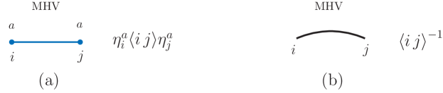
Figure 1: For an MHV amplitude the shaded (blue) “index line” (a) connecting leg $i$ to leg $j$ represents $\langle q_{i}^{a}\,q_{j}^{a}\rangle$. The two endpoints (and line) carry the same $SU(4)$ index. A solid (black) line (b) without endpoint dots represents a spinor product in the denominator.

In addition to the Grassmann delta function, color-ordered MHV amplitudes also have another important structure, the cyclic spinor string in the denominator,

$$(\left\langle 1\,2\right\rangle\left\langle 2\,3\right\rangle\left\langle 3\,4\right\rangle\left\langle 4\,5\right\rangle\ldots\left\langle n\,1\right\rangle)^{-1}.$$ (21)

This object has the same order as the trace of color-group generators, and can be thought of as being in one-to-one correspondence with this color structure. The spinor products in the denominator of MHV amplitudes will be represented by solid (black) lines without endpoint dots shown in fig. 1(b). The cyclicity of the MHV denominator implies that these lines form closed loops, except for the small gaps that we take to represent external states. It is convenient to draw the diagrams in a form reminiscent of string theory world-sheets, as displayed in fig. 2. The main role of the solid (black) lines will be to span the background, or canvas, on which the shaded (blue) $SU(4)$ index lines are drawn. The presentation of amplitudes in this world-sheet-like fashion provides the necessary room to draw the index lines without cluttering the figures. These diagrams—which we will call “index diagrams”—capture the spinor structures of MHV tree amplitudes along with the relative signs encoded by the superspace.

Given an MHV tree $n$-point amplitude with specified external states, the rules for drawing the $SU(4)$ index diagram are simple: First draw the $n$ solid (black) lines representing the cyclic spinor string of the MHV amplitude denominator. Leave $n$ gaps between these lines to represent the external states, or legs. Label these legs with the appropriate momentum, helicity and $SU(4)$ indices. If the same $SU(4)$ index appears on external legs they should be connected by a shaded (blue) line with endpoint dots. This completes the diagram.

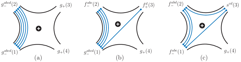
Figure 2: Examples of $SU(4)$ index diagrams for specifying numerator factors of MHV tree amplitudes. The diagrams (a), (b) and (c) correspond to the amplitudes in eq. (22). The shaded (blue) line connecting leg $i$ to leg $j$ represents a factor of $\eta^{a}_{i}\left\langle i\,j\right\rangle\eta^{a}_{j}$ respectively, and solid (black) lines represents $\left\langle i\,j\right\rangle^{-1}$. The white “$+$” label on black background indicates that the amplitude is holomorphic, or MHV.

Consider, for example, the tree amplitudes in eq. (4), whose corresponding diagrams are shown in fig. 2. The “$+$” and “$-$” labels on the external states indicate the helicities, while the black-and-white-inverted “$+$” and “$-$” labels internal to the diagram indicates whether it is an MHV or $\overline{\hbox{MHV}}$ amplitude, respectively. We will refer to this property of being either MHV or $\overline{\hbox{MHV}}$ as an amplitude’s holomorphicity, as MHV amplitudes are built from holomorphic $\lambda^{\alpha}$ spinors and $\overline{\hbox{MHV}}$ amplitudes are constructed from anti-holomorphic $\tilde{\lambda}^{\dot{\alpha}}$ spinors. From the above construction it follows that the index lines in the diagrams of fig. 2 are in one-to-one correspondence to components in the MHV superamplitude, including the Grassmann parameters. Translating from the figures to analytic expressions using the rules of fig. 1, we can easily write down these component amplitudes,

$${\rm(a)}:\;\langle g^{1234}_{-}(1)g^{1234}_{-}(2)g_{+}(3)g_{+}(4)\rangle=i{\prod_{a=1}^{4}\left\langle q^{a}_{1}\,q^{a}_{2}\right\rangle\over\left\langle 1\,2\right\rangle\left\langle 2\,3\right\rangle\left\langle 3\,4\right\rangle\left\langle 4\,1\right\rangle}\,,$$

$${\rm(b)}:\;\langle g^{abcd}_{-}(1)f^{abc}_{-}(2)f^{d}_{+}(3)g_{+}(4)\rangle=i{\left\langle q^{a}_{1}\,q^{a}_{2}\right\rangle\left\langle q^{b}_{1}\,q^{b}_{2}\right\rangle\left\langle q^{c}_{1}\,q^{c}_{2}\right\rangle\left\langle q^{d}_{1}\,q^{d}_{3}\right\rangle\over\left\langle 1\,2\right\rangle\left\langle 2\,3\right\rangle\left\langle 3\,4\right\rangle\left\langle 4\,1\right\rangle}\,,$$

$${\rm(c)}:\;\langle f^{abc}_{-}(1)f^{abd}_{-}(2)s^{cd}(3)g_{+}(4)\rangle=i{\left\langle q^{a}_{1}\,q^{a}_{2}\right\rangle\left\langle q^{b}_{1}\,q^{b}_{2}\right\rangle\left\langle q^{c}_{1}\,q^{c}_{3}\right\rangle\left\langle q^{d}_{2}\,q^{d}_{3}\right\rangle\over\left\langle 1\,2\right\rangle\left\langle 2\,3\right\rangle\left\langle 3\,4\right\rangle\left\langle 4\,1\right\rangle}\,,$$ (22)

where we have labeled the color ordered amplitudes (including Grassmann parameters) using a “correlator” notation on the left hand side. Repeated indices are not summed over their values; rather, their values are fixed and correspond to the particular choice of $SU(4)$ labels identifying the external states. For the amplitude to be nonvanishing, the labels $a,b,c,d$ must be distinct.

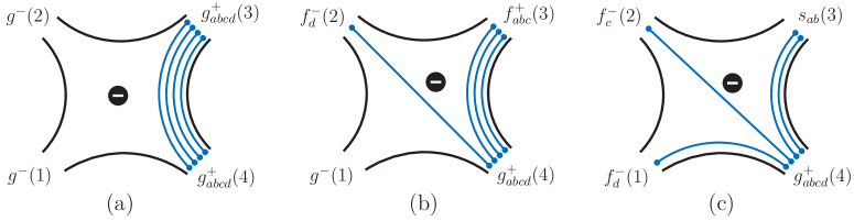
Figure 3: The same amplitudes as in fig. 2, now in the $\overline{\hbox{MHV}}$ representation. The shaded (blue) line connecting leg $i$ to leg $j$ represents a factor of $\widetilde{\eta}_{ia}\left[i\,j\right]\widetilde{\eta}_{ja}$ respectively, and solid (black) lines represents $\left[i\,j\right]^{-1}$. The white “$-$” label on black background indicates that the amplitude is anti-holomorphic, or $\overline{\hbox{MHV}}$.

Diagrams tracking the $SU(4)$ indices for $\overline{\hbox{MHV}}$ amplitudes are similar. As a simple example, consider the same amplitudes as above, but reinterpreted as $\overline{\hbox{MHV}}$ amplitudes—for four-point amplitudes (but no others) this is always possible. In the $\overline{\hbox{MHV}}$ form the amplitudes are,

$${\rm(a)}:\;\langle g^{-}(1)g^{-}(2)g^{+}_{1234}(3)g^{+}_{1234}(4)\rangle=i{\prod_{a=1}^{4}\left[\tilde{q}_{3a}\,\tilde{q}_{4a}\right]\over\left[1\,2\right]\left[2\,3\right]\left[3\,4\right]\left[4\,1\right]}\,,$$

$${\rm(b)}:\;\langle g^{-}(1)f_{d}^{-}(2)f^{+}_{abc}(3)g^{+}_{abcd}(4)\rangle=i{\left[\tilde{q}_{3a}\,\tilde{q}_{4a}\right]\left[\tilde{q}_{3b}\,\tilde{q}_{4b}\right]\left[\tilde{q}_{3c}\,\tilde{q}_{4c}\right]\left[\tilde{q}_{2d}\,\tilde{q}_{4d}\right]\over\left[1\,2\right]\left[2\,3\right]\left[3\,4\right]\left[4\,1\right]}\,,$$

$${\rm(c)}:\;\langle f_{d}^{-}(1)f_{c}^{-}(2)s_{ab}(3)g^{+}_{abcd}(4)\rangle=i{\left[\tilde{q}_{3a}\,\tilde{q}_{4a}\right]\left[\tilde{q}_{3b}\,\tilde{q}_{4b}\right]\left[\tilde{q}_{2c}\,\tilde{q}_{4c}\right]\left[\tilde{q}_{1d}\,\tilde{q}_{4d}\right]\over\left[1\,2\right]\left[2\,3\right]\left[3\,4\right]\left[4\,1\right]}\,,$$ (23)

where $\tilde{q}_{ia}$ are the conjugate supermomenta defined in eq. (13). The index diagrams corresponding to these expressions are displayed in fig. 3. Now the lines are interpreted in terms of conjugate or anti-holomorphic spinors and Grassmann parameters. As mentioned above, this is indicated by the black-and-white-inverted “$-$” label on each $\overline{\hbox{MHV}}$ diagram.

If we wish to work entirely in the $\eta$-superspace for both MHV and $\overline{\hbox{MHV}}$ amplitudes, we must map the $\widetilde{\eta}$ parameters to $\eta$’s using the Grassmann Fourier transform $\widehat{F}$ in eq. (14). This transformation is conveniently captured by the rule in eq. (16), giving,

$${\rm(a)}:\;\widehat{F}\,\langle g^{-}(1)g^{-}(2)g^{+}_{1234}(3)g^{+}_{1234}(4)\rangle=i{\prod_{a=1}^{4}\eta_{1}^{a}\eta_{2}^{a}\left[3\,4\right]\over\left[1\,2\right]\left[2\,3\right]\left[3\,4\right]\left[4\,1\right]}\,,$$

$${\rm(b)}:\;\widehat{F}\,\langle g^{-}(1)f_{d}^{-}(2)f^{+}_{abc}(3)g^{+}_{abcd}(4)\rangle=i{\eta_{1}^{a}\eta_{2}^{a}\left[3\,4\right]\eta_{1}^{b}\eta_{2}^{b}\left[3\,4\right]\eta_{1}^{c}\eta_{2}^{c}\left[3\,4\right]\eta_{1}^{d}\eta_{3}^{d}\left[4\,2\right]\over\left[1\,2\right]\left[2\,3\right]\left[3\,4\right]\left[4\,1\right]}\,,$$

$${\rm(c)}:\;\widehat{F}\,\langle f_{d}^{-}(1)f_{c}^{-}(2)s_{ab}(3)g^{+}_{abcd}(4)\rangle=i{\eta_{1}^{a}\eta_{2}^{a}\left[3\,4\right]\eta_{1}^{b}\eta_{2}^{b}\left[3\,4\right]\eta_{1}^{c}\eta_{3}^{c}\left[4\,2\right]\eta_{2}^{d}\eta_{3}^{d}\left[1\,4\right]\over\left[1\,2\right]\left[2\,3\right]\left[3\,4\right]\left[4\,1\right]}\,.$$ (24)

While perhaps less obvious for the time being, the utility of the index diagrams will become apparent in section V, where they will allow a transparent bookkeeping of the helicity states in unitarity cuts of multi-loop (super)amplitudes.

II.4 MHV superrules for non-MHV superamplitudes

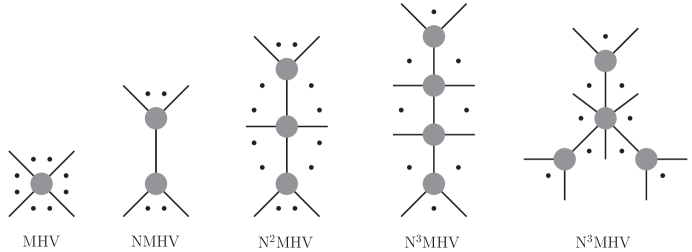
Figure 4: The MHV vertex construction builds non-MHV superamplitudes from MHV superamplitudes. The blobs are MHV superamplitudes, and the dots signify an arbitrary number of external legs, of which a few are drawn explicitly.

The MHV vertex construction generates non-MHV amplitudes from the MHV ones via a set of simple diagrammatic rules. Their validity has been proven in various ways, including the use of on-shell recursion Risager and by realizing the MHV vertex rules as the Feynman rules of a Lagrangian CSW_Lagrangian ; CSW_QCD . The former approach was recently shown to hold, with certain modifications, for all amplitudes of ${{\cal N}=4}$ super-Yang-Mills theory FreedmanProof , proving the validity of the MHV vertex construction for the complete theory. The latter approach was also extended CSW_LagrangianSusy to the complete ${{\cal N}=4}$ Lagrangian by carrying out an ${\cal N}=4$ supersymmetrization of the MHV Lagrangian of refs. CSW_Lagrangian .

The $n$-point N^mMHV gauge theory superamplitude (where the “N” stands for “Next-to-”) contains gluon amplitudes with $(m+2)$ negative helicity gluons. One begins its construction by drawing all tree graphs with $(m+1)$ vertices, on which the external $n$ legs are distributed in all possible inequivalent ways while maintaining the color order. Examples of these graph topologies are shown in fig. 4.

To each vertex one associates an MHV superamplitude (8). As in the bosonic MHV rules, the holomorphic spinor $\lambda_{P}$ associated to an internal leg is constructed from the corresponding off-shell momentum $P$ using an arbitrary (but the same for all graphs) null reference antiholomorphic spinor $\zeta^{\dot{\alpha}}$,

$$\lambda_{P\alpha}\equiv P_{\alpha{\dot{\alpha}}}\zeta^{\dot{\alpha}}\,.$$ (25)

Alternatively, the holomorphic spinor $\lambda_{P}=|P^{\flat}\rangle$ can be defined in terms of a “null projection” of $P$, given by K_proj ; BBK ,

$$P^{\flat}=P-\frac{P^{2}}{2\zeta\cdot P}\zeta\,,$$ (26)

where $\zeta^{\mu}$ is a null reference vector. In this form it is clear that the momenta of every vertex are on shell, thus, at this stage, the expression corresponding to each graph is a simple product of $(m+1)$ well-defined on-shell tree superamplitudes. (The analogous construction for gravity amplitudes is more complicated due to the fact that MHV supergravity amplitudes are not holomorphic GravityMHV .)

To each internal line connecting two vertices one associates a super-propagator which consists of the product between a standard scalar Feynman propagator $i/P^{2}$ and a factor which equates the fermionic coordinates $\eta$ of the internal line in the two vertices connected by it. The structure of the propagator depends on the precise definition of the superspace, but such details are not important for the following. Upon application of the precise rules for assembling the MHV vertex diagrams, the expression for the N^mMHV superamplitude is given by

$${\cal A}^{{\rm N}^{m}{\rm MHV}}_{n}=i^{m}\sum_{\rm all~{}graphs}\int\Bigl{[}\prod_{j=1}^{m}{d^{4}\eta_{j}\over P^{2}_{j}}\Bigr{]}{\cal A}^{\rm MHV}_{(1)}{\cal A}^{\rm MHV}_{(2)}\cdots{\cal A}^{\rm MHV}_{(m)}{\cal A}^{\rm MHV}_{(m+1)}\,,$$ (27)

where the integral is over the $4m$ internal Grassmann parameters ($d^{4}\eta_{j}\equiv\prod_{a=1}^{4}d\eta_{j}^{a}$) associated with the internal legs, and each $P_{j}$ is the (off-shell) momentum of the $j$’th internal leg of the graph. The MHV superamplitudes appearing in the product correspond to the $(m+1)$ vertices of the graph. The momentum and $\eta$ dependence of the MHV superamplitudes is suppressed here. We note, however, that the null projection of each internal momentum $P^{\flat}_{i}$ and the Grassmann variable $\eta_{i}^{a}$ appear twice, in the form,

$$\cdots{\cal A}^{\rm MHV}_{(j)}(P^{\flat}_{i},\eta_{i}^{a})\cdots{\cal A}^{\rm MHV}_{(k)}(-P^{\flat}_{i},\eta_{i}^{a})\cdots$$ (28)

Each integration $\int d^{4}\eta_{i}$ in eq. (27) selects the configurations with exactly four distinct $\eta$-variables $\eta^{1}_{i}\eta^{2}_{i}\eta^{3}_{i}\eta^{4}_{i}$ on each of the internal lines. Since a particular $\eta^{a}_{i}$ can originate from either of two MHV amplitudes, as per eq. (28), there are $2^{4}$ possibilities that may give non-vanishing contributions. These contributions correspond to the 16 states in the ${{\cal N}=4}$ multiplet, making it clear that the application of $\int d^{4}\eta_{i}$ indeed yields the supersum. However, for a given choice of external states, each term corresponding to a distinct graph in (27) receives nonzero contributions from exactly one state for each internal leg.

Note that as far as sewing of amplitudes is concerned, it makes no difference whether an intermediate state is put on-shell due to a cut or due to the MHV vertex expansion. This observation, implying that sewing of general amplitudes proceeds by integrating over common $\eta$ variables, will play an important role in our discussion of cuts of loop amplitudes.

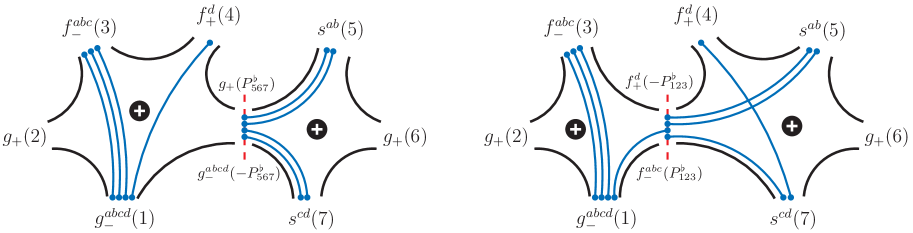
Figure 5: The index lines for two out of the nine diagrams of the MHV vertex expansion for the amplitude $\langle g_{-}^{abcd}(1)g_{+}(2)f_{-}^{abc}(3)f_{+}^{d}(4)s^{ab}(5)g_{+}(6)s^{cd}(7)\rangle$. The dashed vertical (red) line signifies that the intermediate state is on-shell. The integration $\int d^{4}\eta$ will force exactly four $SU(4)$ index lines to end (or start) on the intermediate on-shell state.

We now illustrate the index diagrams, introduced in the previous section, for the MHV-vertex expansion of an NMHV example. Since the index diagrams represent component amplitudes these diagrams clarify the details of the ${{\cal N}=4}$ state sum. First we note that according to eq. (27) an N^mMHV amplitude is a polynomial in $\eta$ of degree $8(m+1)-4m=8+4m$, since there are $(m+1)$ MHV amplitudes—which by definition contain eight $\eta$’s with upper $SU(4)$ indices—and the Grassmann integration removes $4m$ of them. Thus, an NMHV amplitude must have 12 ($3\times 4$ distinct) upper $SU(4)$ indices.

Let us consider the seven-point amplitude $\langle g_{-}^{abcd}(1)g_{+}(2)f_{-}^{abc}(3)f_{+}^{d}(4)s^{ab}(5)g_{+}(6)s^{cd}(7)\rangle$ which is of this form. There are a total of nine non-vanishing diagrams, of which two are displayed as index diagrams in fig. 5, illustrating the sewing of gluonic and fermionic states, respectively. Summing over the diagrams gives us the amplitude

$$\hskip-5.69046pt\langle g_{-}^{abcd}(1)g_{+}(2)f_{-}^{abc}(3)f_{+}^{d}(4)s^{ab}(5)g_{+}(6)s^{cd}(7)\rangle$$

$$\hskip 5.69046pt=\int d^{4}\eta_{P^{\flat}_{567}}\langle g_{-}^{abcd}(1)g_{+}(2)f_{-}^{abc}(3)f_{+}^{d}(4)g_{+}(P^{\flat}_{567})\rangle\frac{i}{(P_{567})^{2}}\langle g_{-}^{abcd}(-P^{\flat}_{567})s^{ab}(5)g_{+}(6)s^{cd}(7)\rangle$$

$$\hskip 14.22636pt\hbox{}+\int d^{4}\eta_{P^{\flat}_{123}}\langle f_{+}^{d}(4)s^{ab}(5)g_{+}(6)s^{cd}(7)f^{abc}_{-}(P^{\flat}_{123})\rangle\frac{i}{(P_{123})^{2}}\langle f_{+}^{d}(-P^{\flat}_{123})g_{-}^{abcd}(1)g_{+}(2)f_{-}^{abc}(3)\rangle$$

$$\hskip 14.22636pt\hbox{}+\cdots$$

$$=-i\frac{\left\langle\smash{q_{1}^{a}}\,\smash{q_{3}^{a}}\right\rangle\left\langle\smash{q_{1}^{b}}\,\smash{q_{3}^{b}}\right\rangle\left\langle\smash{q_{1}^{c}}\,\smash{q_{3}^{c}}\right\rangle\left\langle\smash{q_{1}^{d}}\,\smash{q_{4}^{d}}\right\rangle}{\left\langle\smash{1}\,\smash{2}\right\rangle\left\langle\smash{2}\,\smash{3}\right\rangle\left\langle\smash{3}\,\smash{4}\right\rangle\left\langle\smash{4}\,\smash{P^{\flat}_{567}}\right\rangle\left\langle\smash{P^{\flat}_{567}}\,\smash{1}\right\rangle}\frac{1}{(P_{567})^{2}}\frac{\left\langle\smash{P^{\flat}_{567}}\,\smash{q_{5}^{a}}\right\rangle\left\langle\smash{P^{\flat}_{567}}\,\smash{q_{5}^{b}}\right\rangle\left\langle\smash{P^{\flat}_{567}}\,\smash{q_{7}^{c}}\right\rangle\left\langle\smash{P^{\flat}_{567}}\,\smash{q_{7}^{d}}\right\rangle}{\left\langle\smash{P^{\flat}_{567}}\,\smash{5}\right\rangle\left\langle\smash{5}\,\smash{6}\right\rangle\left\langle\smash{6}\,\smash{7}\right\rangle\left\langle\smash{7}\,\smash{P^{\flat}_{567}}\right\rangle}\hskip 43.24817pt$$

$$\hskip 14.22636pt\hbox{}+i\frac{\left\langle\smash{P^{\flat}_{123}}\,\smash{q_{5}^{a}}\right\rangle\left\langle\smash{P^{\flat}_{123}}\,\smash{q_{5}^{b}}\right\rangle\left\langle\smash{P^{\flat}_{123}}\,\smash{q_{7}^{c}}\right\rangle\left\langle\smash{q_{4}^{d}}\,\smash{q_{7}^{d}}\right\rangle}{\left\langle\smash{4}\,\smash{5}\right\rangle\left\langle\smash{5}\,\smash{6}\right\rangle\left\langle\smash{6}\,\smash{7}\right\rangle\left\langle\smash{7}\,\smash{P^{\flat}_{123}}\right\rangle\left\langle\smash{P^{\flat}_{123}}\,\smash{4}\right\rangle}\frac{1}{(P_{123})^{2}}\frac{\left\langle\smash{q_{1}^{a}}\,\smash{q_{3}^{a}}\right\rangle\left\langle\smash{q_{1}^{b}}\,\smash{q_{3}^{b}}\right\rangle\left\langle\smash{q_{1}^{c}}\,\smash{q_{3}^{c}}\right\rangle\left\langle\smash{P^{\flat}_{123}}\,\smash{q_{1}^{d}}\right\rangle}{\left\langle\smash{P^{\flat}_{123}}\,\smash{1}\right\rangle\left\langle\smash{1}\,\smash{2}\right\rangle\left\langle\smash{2}\,\smash{3}\right\rangle\left\langle\smash{3}\,\smash{P^{\flat}_{123}}\right\rangle}$$

$$\hskip 14.22636pt\hbox{}+\cdots$$ (29)

where,

$$P_{ijl}=k_{i}+k_{j}+k_{l}\,,\hskip 56.9055pt\langle P^{\flat}\,q^{a}_{i}\rangle=\langle P^{\flat}\,i\rangle\eta^{a}_{i}\,,$$ (30)

and we suppress all but the contributions of the two diagrams in fig. 5. In the last equality we carried out the Grassmann integration, which here only serves to convert the internal four powers of $\eta$ to factors of $\pm 1$. When using the MHV diagrams expansion in unitarity cuts of loop amplitudes, as we will see in section IV, it is generally convenient to delay carrying out the Grassmann integrations until the complete cut is assembled.

We note that it is convenient to collect the various N^mMHV tree superamplitudes into a single generating function,

$${\cal A}^{\rm tree}={\cal A}^{\rm MHV}+{\cal A}^{\rm NMHV}+{\cal A}^{\rm N^{2}MHV}+\cdots+{\cal A}^{{\rm N}^{(n-4)}{\rm MHV}}\,,$$ (31)

where $n$ is the number of external legs, and the sum terminates with the $\overline{\hbox{MHV}}$ amplitude, here written as an N^(n-4)MHV amplitude in $\eta$ superspace. The number of terms in this sum is $n-3$ for $n\geq 4$. The three-point case should be treated separately since it contains two terms, MHV and $\overline{\hbox{MHV}}$, which cannot be supported on the same kinematics.

III Evaluation of Loop Amplitudes using the Unitarity Method

The direct evaluation of generalized unitarity cuts of ${\cal N}=4$ super-Yang-Mills scattering amplitudes requires summing over all possible intermediate on-shell states of the theory. Various strategies for carrying out such sums over states have recently been discussed in refs. KorchemskyOneLoop ; AHCKGravity ; FreedmanUnitarity . Here we review our current approach, which is closely related to the generating function ideas of ref. FreedmanGenerating ; FreedmanUnitarity . Additionally, we present an analysis of the structure of the resulting factors and expose various universal features.

III.1 Modern unitarity method

The modern unitarity method gives us a means for systematically constructing multi-loop amplitudes for massless theories. This method and its various refinements have been described in some detail in references UnitarityMethod ; Fusing ; BRY ; GeneralizedUnitarity ; TwoLoopSplit ; BDDPR ; BCFGeneralized ; FiveLoop ; FreddyMaximal , so here we will mainly review points salient to the sums over all intermediate states appearing in maximally supersymmetric theories.

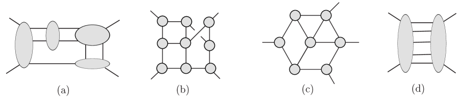
Figure 6: Some examples of generalized cuts at four loops. Every exposed line is cut and satisfies on-shell conditions. Diagrams (b) and(c) are near maximal cuts. In four dimensions only MHV or $\overline{\hbox{MHV}}$ tree amplitudes appear in cuts (a)-(c) while in cut (d) non-MHV tree amplitudes appear.

The construction starts with an ansatz for the amplitude in terms of loop momentum integrals. We require that the numerator of each integral is a polynomial in the loop and external momenta subject to certain constraints, such as the maximum number of factors of loop momenta that can appear. The construction of such an ansatz is simplest for the ${{\cal N}=4}$ super-Yang-Mills four-point amplitudes where it turns out that the ratio between the loop integrand and the tree amplitudes is a rational function solely of Lorentz invariant scalar products BRY ; BCDKS ; FiveLoop . For higher-point amplitudes similar ratios necessarily contain either spinor products or Levi-Civita tensors, as is visible even at one loop UnitarityMethod .

The arbitrary coefficients appearing in the ansatz are systematically constrained by comparing generalized cuts of the ansatz to cuts of the loop amplitude. Particularly useful are cuts composed of $m$ tree amplitudes of form,

$$\sum_{\rm states}A^{\rm tree}_{(1)}A^{\rm tree}_{(2)}A^{\rm tree}_{(3)}\cdots A^{\rm tree}_{(m)}\,,$$ (32)

evaluated using kinematic configurations that place all cut momenta on shell, $l_{i}^{2}=0$. Cuts which break up loop amplitudes into products of tree amplitudes are generally the simplest to work with to determine an amplitude, although one can also use lower-loop amplitudes in the cuts as well. In special cases, such as when there is a four-point subamplitude, this can be advantageous FourLoopNonPlanar . In fig. 6, we display a few unitarity cuts relevant to four loops. If cuts of the ansatz cannot be made consistent with the cuts of the amplitude, then it is, of course, necessary to enlarge the ansatz.

The reconstruction of an amplitude from a single cut configuration is typically ambiguous as the numerator may be freely modified by adding terms which vanish on the cut in question. Consider, for example, a particular two-particle cut with cut momenta labeled $l_{1}$ and $l_{2}$. No expressions proportional to $l_{1}^{2}=0$ and $l_{2}^{2}=0$ are constrained by this particular cut. Such terms are instead constrained by other cuts. After information from all cuts is included, the only remaining ambiguities are terms which are free of cuts in every channel. In the full amplitude these ambiguities add up to zero, representing the freedom to re-express the amplitude into different algebraically equivalent forms. Using this freedom one can find representations with different desirable properties, such as manifest symmetries or explicit power counting GravityThree ; CompactThree .

For multi-loop calculations, generally it is best to organize the evaluation of the cuts following to the method of maximal cuts FiveLoop . In this procedure we start from generalized cuts GeneralizedUnitarity ; TwoLoopSplit ; BCFGeneralized with the maximum number of cut propagators and then systematically reduce the number of cut propagators FiveLoop . This allows us to isolate the missing pieces of the amplitude, as well as reduce the computational complexity of each cut. A related procedure is the “leading-singularity” technique, valid for maximally supersymmetric amplitudes FreddyMaximal ; LeadingApplications . These leading singularities, which include additional hidden singularities, have been suggested to determine any maximally supersymmetric amplitude AHCKGravity .

At one loop, all singular and finite terms in amplitudes of massless supersymmetric theories are determined completely by their four-dimensional cuts Fusing . Unfortunately, no such property has been demonstrated at higher loops, although there is evidence that it holds for four-point amplitudes in this theory through five loops BCDKS ; GravityThree ; FiveLoop . We do not expect that it will continue for higher-point amplitudes. Indeed, we know that for two-loop six-point amplitudes terms which vanish in $D=4$ do appear TwoLoopSixPt . Even at four points, Gram determinants which vanish in four dimensions, but not in $D$-dimensions, could appear at higher-loop orders.

At present, $D$-dimensional evaluation of cuts is required to guarantee that integrand contributions which vanish in four dimensions are not dropped. $D$-dimensional cuts DDimUnitarity make calculations significantly more difficult, because powerful four-dimensional spinor methods SpinorHelicity can no longer be used. (Recently, however, a helicity-like formalism in six dimensions has been given D6Helicity .) Some of this additional complexity is avoided by performing internal-state sums using the (simpler) gauge supermultiplet of $D=10,\,{\cal N}=1$ super-Yang-Mills theory instead of the $D=4,\,{{\cal N}=4}$ multiplet. In any case, it is usually much simpler to verify an ansatz constructed using the simpler four-dimensional analysis, than to construct the amplitude directly from its $D$-dimensional cuts.

For simple four-dimensional cuts, the sum over states in eq. (32), can easily be evaluated in components, making use of supersymmetry Ward identities SWI , as discussed in ref. BDDPR . In some cases, when maximal or nearly maximal number of propagators are cut, it is possible to choose “singlet” kinematics which force all or nearly all particles propagating in the loops to be gluons in the ${{\cal N}=4}$ super-Yang-Mills theory FiveLoop . However, for more general situations, we desire a systematic means for evaluating supersymmetric cuts, such as the generating function approach of ref. FreedmanGenerating ; FreedmanUnitarity .

III.2 General structure of a supercut

Using superamplitudes, integration over the $\eta$ parameters of the cut legs represents the sum over states crossing the cuts in eq. (32). The generalized supercut is given by,

$${\cal C}=\int\Bigl{[}\prod_{i=1}^{k}{d^{4}\eta_{i}}\Bigr{]}{\cal A}^{\rm tree}_{(1)}{\cal A}^{\rm tree}_{(2)}{\cal A}^{\rm tree}_{(3)}\cdots{\cal A}^{\rm tree}_{(m)}\,,$$ (33)

where ${\cal A}_{(j)}^{\rm tree}$ are generating functions (31) connected by $k$ on-shell cut legs. The supercut incorporates all internal and external helicities and particles of the ${{\cal N}=4}$ multiplet. In most cases it is convenient to restrict this cut by choosing external configurations, e.g. external MHV or $\overline{\hbox{MHV}}$ sectors (or even external helicities), etc. In many cases it is also convenient to expand out each ${\cal A}^{\rm tree}$ into its N^mMHV components, and consider each term–consisting of a product of such amplitudes—as a separate contribution. We will focus our analysis on such single terms, since as we will see they form naturally distinct contributions, each being an $SU(4)$ invariant KorchemskyOneLoop expression. As these contributions correspond to internal quantities they must be summed over. We note that although in this discussion we restrict to cuts containing only trees, it can sometimes be advantageous to consider cuts containing also four and five-point loop amplitudes, since they satisfy the same supersymmetry relations as the tree-level amplitudes.

If all tree amplitudes in the supercut have fewer than six legs then each supercut contribution is of the form,

$$\int\Bigl{[}\prod_{i=1}^{k}{d^{4}\eta_{i}}\Bigr{]}{\cal A}^{\rm MHV}_{(1)}\cdots{\cal A}^{\rm MHV}_{(m^{\prime})}\hat{\cal A}^{\rm\overline{MHV}}_{(m^{\prime}+1)}\cdots\hat{\cal A}^{\rm\overline{MHV}}_{(m)}\,,$$ (34)

where $\hat{\cal A}^{\rm\overline{MHV}}=\widehat{F}{\cal A}^{\rm\overline{MHV}}$ uses the Grassmann Fourier transform $\widehat{F}$ in eq. (14). For cuts where there are tree amplitudes with more than five legs present, some cut contributions include non-MHV tree amplitudes. For these we apply the MHV vertex expansion (27), which reduces these more complicated cases down to a sum of similar expressions as eq. (34) with only MHV and $\overline{\hbox{MHV}}$ amplitudes (and additional propagators).

Certain properties of the ${{\cal N}=4}$ super-Yang-Mills cuts can be inferred from the structure of generalized cuts and the manifest $R$-symmetry and supersymmetry of tree-level superamplitudes. First we note that a cut contribution that corresponds to a product of only MHV tree amplitudes consists of a single term of the following numerator structure,

$$\int\Bigr{[}\prod_{i}d^{4}\eta_{i}\Bigr{]}\prod_{I}\biggl{(}\,\prod_{a=1}^{4}\delta^{(2)}(Q^{a}_{I})\biggl{)}=\prod_{a=1}^{4}\biggl{(}\int\Bigr{[}\prod_{i}d\eta_{i}^{a}\Bigr{]}\prod_{I}\delta^{(2)}(Q^{a}_{I})\biggr{)}\,,$$ (35)

where we have made it explicit that the product over the $SU(4)$ indices can be commuted past both the product over internal cut legs $i$ and the product over tree amplitudes labeled by $I$. Here $Q_{I}^{a}=\sum_{j}\lambda_{j}\eta^{a}_{j}$ is the total supermomentum of superamplitude ${\cal A}_{I}$, where $j$ runs over all legs of ${\cal A}_{I}$. For convenience we have also suppressed the spinor index. From the right-hand-side of eq. (35), we conclude that the numerator factor arising from the supersum of a cut contribution composed of only MHV amplitudes is simply the fourth power of the numerator factor arising from treating the index in $\eta^{a}$ as taking on only a single value.

A cut contribution constructed from only MHV and $\overline{\rm MHV}$ tree amplitudes has similar structure, though the details are slightly different. Using the fermionic Fourier transform operator (14) any $n$-point $\overline{\rm MHV}$ tree amplitude can manifestly be written as a product over four identical factors, each depending on only one value of the $R$-symmetry index,

$$\prod_{a=1}^{4}\;\int\Bigl{[}\prod_{j}^{n}d\widetilde{\eta}_{ja}e^{\eta^{a}_{j}\widetilde{\eta}_{ja}}\Bigr{]}\,\delta^{(2)}\Bigl{(}\sum_{j=1}^{n}\tilde{\lambda}_{j}\widetilde{\eta}^{a}_{j}\Bigr{)}\,.$$ (36)

Consequently, just as for cut contributions constructed solely from MHV tree amplitudes, for the cases where only MHV and $\overline{\hbox{MHV}}$ tree amplitudes appear in a cut, the end result is that the fourth power of some combination of spinor products appears in the numerator. This feature will play an important role in section V, simplifying the index diagrams that track the $R$-symmetry indices.

The super-MHV vertex expansion generalizes this structure to generic cuts of ${{\cal N}=4}$ loop amplitudes. As already mentioned, any non-MHV tree superamplitude can be expanded as a sum of products of MHV superamplitudes. If we insert this expansion into a generalized cut, we obtain a sum of terms where the structure of each term is the same as a cut contribution composed purely of MHV amplitudes. All that changes is that the momenta carried by some spinors are shifted according to eq. (26), and some internal propagators are made explicit. We immediately deduce that the numerator of each term is given by a fourth power of the numerator factor arising when treating the index of $\eta^{a}$ as having a single value. This general observation is consistent with results found in ref. FreedmanUnitarity .

The structure of the constraints due to supersymmetry may be further disentangled. It is not difficult to see that the cut of any ${{\cal N}=4}$ super-Yang-Mills multi-loop amplitude is proportional to the overall super-momentum conservation constraint on the external supermomenta. Similar observations have been used in a related context in ref. RSV_3 ; KorchemskyOneLoop ; FreedmanProof . This property is a consequence of supersymmetry being preserved by the sewing, which is indeed manifest on the cut, as we now show. Consider an arbitrary generalized cut constructed entirely from tree-level amplitudes; using the MHV-vertex super-rules, this cut may be further decomposed into a sum of products of MHV tree amplitudes. Each term in this sum contains a product of factors of the type (9), one for each MHV amplitude in the product. Using the identity $\delta(A)\delta(B)=\delta(A+B)\delta(B)$ each such product of delta functions may be reorganized by adding to the argument of one of them the arguments of all the other delta functions:

$$\prod_{I=1}^{m}\delta^{(8)}(Q_{I}^{a})=\delta^{(8)}\Bigl{(}\sum_{I=1}^{m}Q_{I}^{a}\Bigr{)}\prod_{I=2}^{m}\delta^{(8)}(Q_{I}^{a})\,,$$ (37)

where $m$ is the number of MHV trees amplitudes—including those from a single graph of each MHV-vertex expansion. In the conventions (7) in which a change of the sign of the four-momentum $p_{i}$ translates to a change of sign of the holomorphic spinor $\lambda_{i}$, and therefore also in $q^{a}_{i}=\lambda_{i}\eta^{a}_{i}$, we immediately see that in the first delta function all $q^{a}_{i}$ corresponding to internal lines occurs pairwise with opposite sign, and thus cancel, leaving only external variables,

$$\delta^{(8)}\Bigl{(}\sum_{I=1}^{m}Q_{I}^{a}\Bigr{)}=\delta^{(8)}\Bigl{(}\sum_{i\in{\cal E}}\lambda_{i}\eta^{a}_{i}\Bigr{)}\,,$$ (38)

where ${\cal E}$ denotes the set of external legs of the loop amplitude whose cut one is computing. Thus, this delta function depends only on the external momentum configuration and is therefore common to all terms appearing in this cut. The generalized cuts involving only tree amplitudes are sufficient for reconstructing the complete loop amplitude TwoLoopSplit , therefore it is clear that the superamplitude and all of its cuts are proportional to $\delta^{(8)}(Q^{a}_{\cal E})$, assuming four-dimensional kinematics.

As can be seen from eqs. (18) and (19), the discussion above, showing supermomentum conservation, goes through unchanged for cuts containing $n$-point tree-level $\overline{\rm MHV}$ amplitudes with $n\geq 4$. This includes all cuts with real momenta. For $n=3$, from ref. KorchemskyOneLoop , we see that the supermomentum conservation constraint of three-point amplitudes may be obtained from their fermionic constraint upon multiplication by a spinor corresponding to one of the external lines. Using this observation, it is then straightforward to show that for $n=3$ eqs. (37) and (38) continue to hold.

The explicit presence of the overall supermomentum conservation constraint eq. (38) is sufficient to exhibit the finiteness Mandelstam of ${{\cal N}=4}$ super-Yang-Mills theory. Since, as we argued, the same overall delta function appears in all cuts, it follows that the complete amplitude also has it as an overall factor. In fact, there is a strong similarity between the superficial power counting that results from this and the super-Feynman diagrams of an off-shell $N=2$ superspace. Indeed, the count corresponds to what we would obtain from the Feynman rules of a superspace form of the MHV Lagrangian CSW_LagrangianSusy which manifestly preserves half of the supersymmetries.

More concretely, for any renormalizable gauge theory with no more than one power of loop momentum at each vertex, the superficial degree of divergence is,

$$d_{s}=4-E+(D-4)L-p\,,$$ (39)

where $L$ is the number of loops, $D$ the dimension, $E$ the number of external legs and $p$ the number of powers of momentum that can be algebraically extracted from the integrals as external momenta. For each power of numerator loop momentum that can be converted to an external momentum, the superficial degree is reduced by one unit. Taking $D=4$ and $p=4$, corresponding to the four powers of external momentum implicit in the overall delta function (38), we see that $d_{s}<0$ for all loops and legs. This also implies that ${{\cal N}=4}$ super-Yang-Mills amplitudes cannot contain any subdivergences as all previous loop orders are finite. It then follows inductively that the negative superficial degree of divergence, for all loop amplitudes, is sufficient to demonstrate the cancellations needed for all order finiteness. We note that although this displays the finiteness of ${{\cal N}=4}$ super-Yang-Mills theory, not all cancellations are manifest, and there are additional ones reducing the degree of divergence beyond those needed for finiteness BDDPR ; FiveLoop ; HoweStelleNew .

A similar analysis can be carried out for ${{\cal N}=8}$ supergravity; in this case the two-derivative coupling leads to a superficial degree of divergence which monotonically increases with the loop order. Without additional mechanisms for taming its ultraviolet behavior, this would lead to the conclusion of that the theory is ultraviolet divergent. As discussed in refs. Finite ; GravityThree ; CompactThree direct evidence to all loop orders indeed points to the existence of much stronger ultraviolet cancellations.

IV The supersum as a system of linear equations

We now address the question of how to best carry out the evaluation of multiple fermionic integrals, which can become tedious for complicated multi-loop cuts. An approach to organizing this calculation, discussed in the following sections, is to devise effective diagrammatic rules for carrying out these integrals. Another complementary approach, discussed in this section, relies on the observation that the fermionic delta functions may be interpreted as a system of linear equations determining the integration variables (i.e. the variables $\eta$ corresponding to the cut lines) in terms of the variables $\eta$ associated with the external lines of the amplitude. From this standpoint, the integral over the internal $\eta$’s may be carried out by directly solving an appropriately chosen system of equations and evaluating the remaining supersymmetry constraints on the solutions of this system. While the relation between the fermionic integrals and the sum over intermediate states in the cuts is quite transparent, as we will see in later sections, it is rather obscure to identify the contribution of one particular particle configuration crossing the cut in the solution of the linear system.

IV.1 Cuts involving MHV and MHV vertex expanded trees

Simple counting shows that after the overall supermomentum conservation constraint is extracted, the number of equations appearing in cuts of MHV amplitudes equals the number of integration variables. For such cuts the result of the Grassmann integration is then just the determinant of the matrix of coefficients of that linear system. The same counting shows that the number of fermionic constraints appearing in cuts of N^kMHV amplitudes is larger than the number of integration variables. One way to evaluate the integral is to determine the integration variables by solving some judiciously chosen subset of the supermomentum constraints and substitute the result into the remaining fermionic delta functions. Care must be taken in selecting the constraints being solved, as an arbitrary choice may obscure the symmetries of the amplitude. One approach is to take the average over all possible subsets of constraints determining all internal fermionic variables. Another general strategy is to select the fermionic constraints with as few external momenta as possible. Since the integration variables are determined as ratio of determinants, all identities based on over-antisymmetrization of Lorentz indices, such as Schouten’s identity, are accounted for automatically, generally yielding simple expressions.

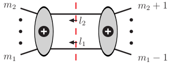
Figure 7: Supercut of a one-loop $n$-point MHV amplitude. The white “$+$” labels on the black background signify that these blobs are holomorphic vertices, or MHV superamplitudes. The dashed (red) line marks the cut, enforcing that momenta crossing the cut are on shell.

To illustrate this approach let us consider the example, shown in fig. 7, of the supercut of the one-loop $n$-point MHV superamplitude

$${\cal C}^{{\rm fig.\ }\ref{OneLoopCutSuperSumFigure}}=\int d^{4}\eta_{l_{1}}\int d^{4}\eta_{l_{2}}\,{\cal A}^{\rm MHV}(-l_{1},m_{1},\dots,m_{2},-l_{2}){\cal A}^{\rm MHV}(l_{2},m_{2}+1,\ldots,m_{1}-1,l_{1})\,.$$ (40)

The only contribution to this cut is where both tree superamplitudes are MHV; together they contain the two delta functions,

$$\delta^{(8)}\Bigl{(}-\lambda_{l_{1}}^{\alpha}\eta_{l_{1}}^{a}-\lambda_{l_{2}}^{\alpha}\eta_{l_{2}}^{a}+\sum_{i=m_{1}}^{m_{2}}\lambda_{i}^{\alpha}\eta_{i}^{a}\Bigr{)}\;\delta^{(8)}\Bigl{(}\lambda_{l_{1}}^{\alpha}\eta_{l_{1}}^{a}+\lambda_{l_{2}}^{\alpha}\eta_{l_{2}}^{a}+\sum_{i=m_{2}+1}^{m_{1}-1}\lambda_{i}^{\alpha}\eta_{i}^{a}\Bigr{)}\,.$$ (41)

Adding the argument of the first delta function to the second one, as discussed in (37), exposes the overall supermomentum conservation

$$\delta^{(8)}\Bigl{(}-\lambda_{l_{1}}^{\alpha}\eta_{l_{1}}^{a}-\lambda_{l_{2}}^{\alpha}\eta_{l_{2}}^{a}+\sum_{i=m_{1}}^{m_{2}}\lambda_{i}^{\alpha}\eta_{i}^{a}\Bigr{)}\;\delta^{(8)}\Bigl{(}\sum_{i=m_{2}+1}^{m_{1}-1}\lambda_{i}^{\alpha}\eta_{i}^{a}+\sum_{i=m_{1}}^{m_{2}}\lambda_{i}^{\alpha}\eta_{i}^{a}\Bigr{)}\,;$$ (42)

then, the value of the fermionic integral in eq. (40) is the determinant of the matrix of coefficients of the following system of linear equations,

$$\lambda_{l_{1}}^{\alpha}\eta_{l_{1}}^{a}+\lambda_{l_{2}}^{\alpha}\eta_{l_{2}}^{a}=\sum_{i=m_{1}}^{m_{2}}\lambda_{i}^{\alpha}\eta_{i}^{a}\,,$$ (43)

interpreted as a system of equations for $\eta_{l_{1}}^{a}$ and $\eta_{l_{2}}^{a}$; its determinant is

$$J = \det{}^{\!4}\left|\begin{array}[]{cc}\lambda_{l_{1}}^{1}&\lambda_{l_{2}}^{1}\\ \lambda_{l_{1}}^{2}&\lambda_{l_{2}}^{2}\end{array}\right|=\langle l_{1}l_{2}\rangle^{4}\,.$$ (46)

Thus, the resulting cut superamplitude is just

$${\cal C}^{{\rm fig.\ }\ref{OneLoopCutSuperSumFigure}} = -\delta^{(8)}\Bigl{(}\sum_{i=1}^{n}\lambda_{i}^{\alpha}\eta_{i}^{a}\Bigr{)}\,\langle l_{1}l_{2}\rangle^{4}\,\times\frac{1}{\langle m_{2}l_{2}\rangle\,\langle l_{2}l_{1}\rangle\,\langle l_{1}m_{1}\rangle\,\prod_{i=m_{1}}^{m_{2}-1}\langle i(i+1)\rangle}$$ (47)

$$\hskip 85.35826pt\times\frac{1}{\langle(m_{1}-1)l_{1}\rangle\,\langle l_{1}l_{2}\rangle\,\langle l_{2}(m_{2}+1)\rangle\,\prod_{i=m_{2}+1}^{m_{1}-2}\langle i(i+1)\rangle}\,.\hskip 28.45274pt$$

Extracting the gluon component we immediately recover the results of reference UnitarityMethod , which had been obtained by using supersymmetry Ward identities SWI and explicitly summing over states crossing the cut.

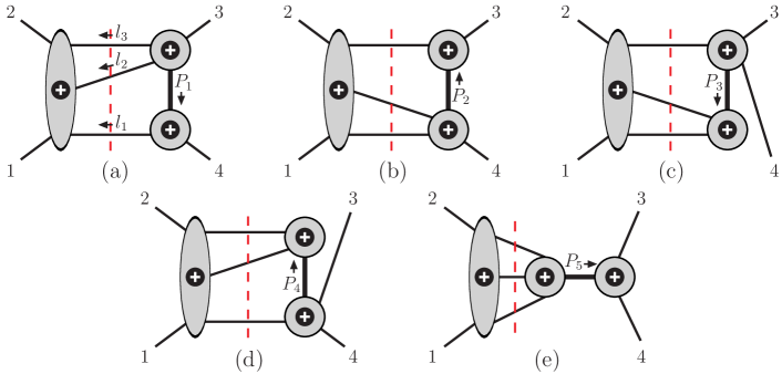
Figure 8: A three-particle supercut for the MHV four-gluon amplitude. This cut contribution contains one MHV and one NMHV superamplitude. The five-point NMHV amplitude is actually $\overline{\hbox{MHV}}$ but it is expanded using the MHV super-rules. The thick line labeled by $P$ marks the internal propagator. Five additional contributions—not shown here—correspond to legs 1 and 2 belonging to an ${\overline{\rm MHV}}$ amplitude and legs 3 and 4 to an MHV amplitude.

Let us now illustrate the interplay between supersum calculations and the super-MHV vertex expansion. The three-particle cut of the two-loop four-gluon amplitude provides the simplest example in this direction, as it contains an $\overline{\hbox{MHV}}$ tree-level amplitude which may be expanded in terms of MHV vertices, as shown in fig. 8. We will describe in detail the supercut contribution in fig. 8(a) and quote the result for the other ones in the figure. Besides the contributions shown in fig. 8 there are additional contributions which sum to the complex conjugate of these, ignoring an overall four-point tree superamplitude factor.

The general strategy is to explicitly write down the constraints for a single value of the $R$-symmetry index and then raise the final result to the fourth power, as discussed in section III.2. We find for fig. 8(a) the following three supermomentum constraints at each of the three MHV vertices,

$$\delta^{(2)}(\lambda_{1}^{\alpha}\eta_{1}^{a}+\lambda_{2}^{\alpha}\eta_{2}^{a}-\lambda_{l_{1}}^{\alpha}\eta_{l_{1}}^{a}-\lambda_{l_{2}}^{\alpha}\eta_{l_{2}}^{a}-\lambda_{l_{3}}^{\alpha}\eta_{l_{3}}^{a})\,\delta^{(2)}(\lambda_{3}^{\alpha}\eta_{3}^{a}+\lambda_{P_{1}}^{\alpha}\eta_{P_{1}}^{a}+\lambda_{l_{2}}^{\alpha}\eta_{l_{2}}^{a}+\lambda_{l_{3}}^{\alpha}\eta_{l_{3}}^{a})$$ (48)

$$\times\delta^{(2)}(\lambda_{4}^{\alpha}\eta_{4}^{a}+\lambda_{l_{1}}^{\alpha}\eta_{l_{1}}^{a}-\lambda_{P_{1}}^{\alpha}\eta_{P_{1}}^{a})\,.$$ (49)

As before, we first isolate the overall supermomentum conservation constraint by adding to the argument of the first delta function the arguments of the second and third ones and noticing the cancellation of all spinors corresponding to the internal lines. The remaining system of four equations involving the fermionic variables for the internal lines are the arguments of the second and third delta functions in equation (49),

$$-\lambda_{P_{1}}^{\alpha}\eta_{P_{1}}^{a}\hphantom{+\lambda_{l_{1}}^{\alpha}\eta_{l_{1}}^{a}}-\lambda_{l_{2}}^{\alpha}\eta_{l_{2}}^{a}-\lambda_{l_{3}}^{\alpha}\eta_{l_{3}}^{a} = \lambda_{3}^{\alpha}\eta_{3}^{a}\,,$$ (50)

$$+\lambda_{P_{1}}^{\alpha}\eta_{P_{1}}^{a}-\lambda_{l_{1}}^{\alpha}\eta_{l_{1}}^{a}\hphantom{-\lambda_{l_{2}}^{\alpha}\eta_{l_{2}}^{a}-\lambda_{l_{3}}^{\alpha}\eta_{l_{3}}^{a}} = \lambda_{4}^{\alpha}\eta_{4}^{a}\,.$$ (51)

Its matrix of coefficients is

$$\begin{pmatrix}-\lambda_{P_{1}}^{\alpha}&0&-\lambda_{l_{2}}^{\alpha}&-\lambda_{l_{3}}^{\alpha}\cr+\lambda_{P_{1}}^{\alpha}&-\lambda_{l_{1}}^{\alpha}&0&0\end{pmatrix}\,,$$ (52)

where each spinor $\lambda^{\alpha}_{j}$ should be thought of as a submatrix with two rows and one column. The determinant of this matrix is just $(\langle l_{1}P^{\flat}_{1}\rangle\langle l_{2}l_{3}\rangle)$. After restoring the four identical factors we thus find that the supersum evaluates to

$$(\langle l_{1}P^{\flat}_{1}\rangle\langle l_{2}l_{3}\rangle)^{4}\delta^{(8)}(\lambda_{1}^{\alpha}\eta_{1}^{a}+\lambda_{2}^{\alpha}\eta_{2}^{a}+\lambda_{3}^{\alpha}\eta_{3}^{a}+\lambda_{4}^{\alpha}\eta_{4}^{a})\,.$$ (53)

In obtaining this simple form, the explicit application of Schouten’s identity was not required.

Carrying out the same steps for the other four components (b), (c), (d) and (e) in fig. 8 gives us the complete expression for this cut contribution,

$$\hskip-8.5359pt{\cal C}^{{\rm fig.\ }\ref{ThreeCutSuperSumFigure}} = \,\delta^{(8)}(\lambda_{1}^{\alpha}\eta_{1}^{a}+\lambda_{2}^{\alpha}\eta_{2}^{a}+\lambda_{3}^{\alpha}\eta_{3}^{a}+\lambda_{4}^{\alpha}\eta_{4}^{a})$$ (54)

$$\times \frac{1}{\langle 12\rangle\langle 2l_{3}\rangle\langle l_{3}l_{2}\rangle\langle l_{2}l_{1}\rangle\langle l_{1}1\rangle}\biggl{[}\frac{1}{\langle l_{2}l_{3}\rangle\langle l_{3}3\rangle\langle 3P^{\flat}_{1}\rangle\langle P^{\flat}_{1}l_{2}\rangle}\frac{1}{P_{1}^{2}}\frac{1}{\langle 4l_{1}\rangle\langle l_{1}P^{\flat}_{1}\rangle\langle P^{\flat}_{1}4\rangle}\left(\langle l_{1}P^{\flat}_{1}\rangle\langle l_{2}l_{3}\rangle\right)^{4}$$

$$\hbox{}\hskip 56.9055pt+\frac{1}{\langle P^{\flat}_{2}l_{3}\rangle\langle l_{3}3\rangle\langle 3P^{\flat}_{2}\rangle}\frac{1}{P_{2}^{2}}\frac{1}{\langle l_{2}P^{\flat}_{2}\rangle\langle P^{\flat}_{2}4\rangle\langle 4l_{1}\rangle\langle l_{1}l_{2}\rangle}\left(\langle l_{3}P^{\flat}_{2}\rangle\langle l_{1}l_{2}\rangle\right)^{4}$$

$$\hbox{}\hskip 56.9055pt+\frac{1}{\langle l_{3}3\rangle\langle 34\rangle\langle 4P^{\flat}_{3}\rangle\langle P^{\flat}_{3}l_{3}\rangle}\frac{1}{P_{3}^{2}}\frac{1}{\langle P^{\flat}_{3}l_{1}\rangle\langle l_{1}l_{2}\rangle\langle l_{2}P^{\flat}_{3}\rangle}\left(\langle l_{3}P^{\flat}_{3}\rangle\langle l_{1}l_{2}\rangle\right)^{4}$$

$$\hbox{}\hskip 56.9055pt+\frac{1}{\langle l_{2}l_{3}\rangle\langle l_{3}P^{\flat}_{4}\rangle\langle P^{\flat}_{4}l_{2}\rangle}\frac{1}{P_{4}^{2}}\frac{1}{\langle l_{1}P^{\flat}_{4}\rangle\langle P^{\flat}_{4}3\rangle\langle 34\rangle\langle 4l_{1}\rangle}\left(\langle l_{1}P^{\flat}_{4}\rangle\langle l_{2}l_{3}\rangle\right)^{4}\biggr{]}\,,\hskip 28.45274pt$$

where,

$$P_{1}=k_{4}+l_{1}\,,\hskip 19.91684ptP_{2}=k_{3}+l_{3}\,,\hskip 19.91684ptP_{3}=l_{1}+l_{2}\,,\hskip 19.91684ptP_{4}=l_{2}+l_{3}\,,$$ (55)

and $P^{\flat}$ is defined in eq. (26). Diagram (e) in fig. 8 gives a vanishing contribution. The dependence on the reference vector $\zeta$ cancels out in eq. (54), as is simple to verify numerically. This expression, together with the five additional contribution (not shown in fig. 8) arising from legs 1 and 2 belonging to an $\overline{\hbox{MHV}}$ amplitude and legs 3 and 4 to an MHV amplitude, numerically agrees with the three-particle cut of the known planar two-loop four-point amplitude BRY ; BDDPR .

IV.2 Cuts with both MHV and $\overline{\hbox{MHV}}$ trees

While the result obtained above is correct, the complexity of eq. (54) is somewhat unsettling. This complexity comes from expanding the $\overline{\hbox{MHV}}$ amplitude in MHV diagrams. For generic non-MHV diagrams this strategy is useful, but for $\overline{\hbox{MHV}}$ amplitudes there is no need to do so. Indeed previous evaluations of the above cut BRY ; BDDPR ; FreedmanUnitarity without making use of the MHV expansion give simpler forms. In the same spirit, it is sometimes convenient to use the $\overline{\hbox{MHV}}$ representation of four-point amplitudes. As illustrated in fig. 9, we therefore reconsider the previous example shown in fig. 8, but without expanding the $\overline{\hbox{MHV}}$ amplitude in MHV amplitudes.

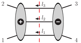
Figure 9: The same three-particle cut contribution as in fig. 8, but where the right-hand-side $\overline{\hbox{MHV}}$ amplitude is not expanded using the MHV rules. The “$+$” label signifies a holomorphic vertex, or MHV superamplitude, and the “$-$” label signifies a anti-holomorphic vertex, or $\overline{\hbox{MHV}}$ superamplitude.

The relevant fermionic integral (where we again keep explicitly a single $R$-symmetry index and raise the result to the fourth power) is,

$$\int d\eta^{a}_{l_{1}}d\eta^{a}_{l_{2}}d\eta^{a}_{l_{3}}d^{2}\omega^{a}\;\delta^{(2)}(\lambda_{1}^{\alpha}\eta_{1}^{a}+\lambda_{2}^{\alpha}\eta_{2}^{a}-\lambda_{l_{1}}^{\alpha}\eta_{l_{1}}^{a}-\lambda_{l_{2}}^{\alpha}\eta_{l_{2}}^{a}-\lambda_{l_{3}}^{\alpha}\eta_{l_{3}}^{a})$$ (56)

$$~{}~{}~{}~{}~{}~{}~{}~{}\times\delta(\eta^{a}_{l_{1}}-{\tilde{\lambda}}^{\dot{\alpha}}_{l_{1}}\omega^{a}_{\dot{\alpha}})\,\delta(\eta^{a}_{l_{2}}-{\tilde{\lambda}}^{\dot{\alpha}}_{l_{2}}\omega^{a}_{\dot{\alpha}})\,\delta(\eta^{a}_{l_{3}}-{\tilde{\lambda}}^{\dot{\alpha}}_{l_{3}}\omega^{a}_{\dot{\alpha}})\,\delta(\eta^{a}_{3}-{\tilde{\lambda}}^{\dot{\alpha}}_{3}\omega^{a}_{\dot{\alpha}})\,\delta(\eta^{a}_{4}-{\tilde{\lambda}}^{\dot{\alpha}}_{4}\omega^{a}_{\dot{\alpha}})\,.\hskip 28.45274pt$$ (57)

Here $\omega^{a}_{\dot{\alpha}}$ are the auxiliary integration variables in equation (18). Adding the arguments of the delta functions on the second line, with the appropriate weights, to the argument of the delta function on the first line exposes the overall supermomentum conservation. We are then left with

$$\delta^{(2)}(\lambda_{1}^{\alpha}\eta_{1}^{a}+\lambda_{2}^{\alpha}\eta_{2}^{a}+\lambda_{3}^{\alpha}\eta_{3}^{a}+\lambda_{4}^{\alpha}\eta_{4}^{a})$$ (58)

$$\times\int d\eta^{a}_{l_{1}}d\eta^{a}_{l_{2}}d\eta^{a}_{l_{3}}d^{2}\omega^{a}\delta(\eta^{a}_{l_{1}}-{\tilde{\lambda}}^{\dot{\alpha}}_{l_{1}}\omega^{a}_{\dot{\alpha}})\,\delta(\eta^{a}_{l_{2}}-{\tilde{\lambda}}^{\dot{\alpha}}_{l_{2}}\omega^{a}_{\dot{\alpha}})\,\delta(\eta^{a}_{l_{3}}-{\tilde{\lambda}}^{\dot{\alpha}}_{l_{3}}\omega^{a}_{\dot{\alpha}})\,\delta(\eta^{a}_{3}-{\tilde{\lambda}}^{\dot{\alpha}}_{3}\omega^{a}_{\dot{\alpha}})\,\delta(\eta^{a}_{4}-{\tilde{\lambda}}^{\dot{\alpha}}_{4}\omega^{a}_{\dot{\alpha}})\,.$$

The matrix of coefficients of the surviving system of constraints can be easily read off,

$$\begin{pmatrix}1&0&0&-{\tilde{\lambda}}^{\dot{1}}_{l_{1}}&-{\tilde{\lambda}}^{\dot{2}}_{l_{1}}\\ 0&1&0&-{\tilde{\lambda}}^{\dot{1}}_{l_{2}}&-{\tilde{\lambda}}^{\dot{2}}_{l_{2}}\\ 0&0&1&-{\tilde{\lambda}}^{\dot{1}}_{l_{3}}&-{\tilde{\lambda}}^{\dot{2}}_{l_{3}}\\ 0&0&0&-{\tilde{\lambda}}^{\dot{1}}_{3}&-{\tilde{\lambda}}^{\dot{2}}_{3}\\ 0&0&0&-{\tilde{\lambda}}^{\dot{1}}_{4}&-{\tilde{\lambda}}^{\dot{2}}_{4}\end{pmatrix}\,.$$ (59)

Taking its determinant, raising it to the fourth power, and restoring the remaining factors in the tree-level superamplitudes gives the supercut contribution,

$${\cal C}^{{\rm fig.}\ \ref{ThreeCutSuperSumMHVbarFigure}}=\delta^{(8)}\Bigl{(}\sum_{i=1}^{4}\lambda_{i}^{\alpha}\eta_{i}^{a}\Bigr{)}\,[34]^{4}\,\frac{1}{\langle 12\rangle\langle 2l_{3}\rangle\langle l_{3}l_{2}\rangle\langle l_{2}l_{1}\rangle\langle l_{1}1\rangle}\frac{1}{[34][4l_{1}][l_{1}l_{2}][l_{2}l_{3}][l_{3}3]}\,.$$ (60)

This numerically matches eq. (54), again giving the proper contribution to the cut four-gluon amplitude at two loops BRY ; BDDPR .

This calculation illustrates a general feature of supersums: if an $\overline{\hbox{MHV}}$ vertex appearing in a supercut has two external legs attached to it, say $p$ and $k$, such as legs $3$ and $4$ in the example above, then apart from the overall supermomentum conservation, the supercut contribution is also proportional to the bracket product of those two momenta, i.e. it contains a numerator factor,

$$\delta^{(8)}\Bigl{(}\sum_{i\in{\cal E}}\lambda_{i}^{\alpha}\eta^{a}_{i}\Bigr{)}\,[pk]^{4}\,.$$ (61)

As in eq. (38), $\cal E$ denotes the set of external legs. This feature is related to the soft ultraviolet properties of ${{\cal N}=4}$ super-Yang-Mills theory.

The $\overline{\hbox{MHV}}$ superamplitudes can also be used in the cuts in conjunction with the MHV-vertex rules. Indeed, any on-shell four-point amplitude may be interpreted either as MHV or $\overline{\hbox{MHV}}$ amplitudes as can be seen by directly evaluating the $\omega$ integral in equation (18) for $n=4$:

$$\widehat{F}{\cal A}^{\overline{\rm MHV}}_{4}=i\delta^{(8)}\Bigl{(}\sum_{i=1}^{4}\lambda_{i}^{\alpha}\eta^{a}_{i}\Bigr{)}\frac{[34]^{4}}{\langle 12\rangle^{4}[12][23][34][41]}=i\delta^{(8)}\Bigl{(}\sum_{i=1}^{4}\lambda_{i}^{\alpha}\eta^{a}_{i}\Bigr{)}\frac{1}{\langle 12\rangle\langle 23\rangle\langle 34\rangle\langle 41\rangle}\,.$$ (62)

Depending on context, choosing one interpretation of the four-point amplitude over the other can lead to more factors of loop momenta in supersums being replaced by factors of external momenta thus making manifest more of the supersymmetric cancellations. We will comment on an example in this direction at the end of section IV.3.

IV.3 Cuts of higher-point superamplitudes

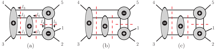
Figure 10: A generalized cut for a four-loop five-point MHV superamplitude having three cut contributions (a), (b) and (c), corresponding to three independent choices of holomophicity of the tree amplitudes comprising the cut.

The above techniques are by no means restricted to four-point amplitudes. To illustrate this, consider the supercut of the MHV four-loop five-point amplitude shown in fig. 10. For the displayed cut topology, these are the three independent non-vanishing assignments of MHV or $\overline{\hbox{MHV}}$ configurations that contribute to an external MHV configuration. (Changing the MHV to an $\overline{\hbox{MHV}}$ label on the lone four-point amplitude is not an independent choice, as the two cases are equivalent.)

For the cut contribution in figure 10(a) the Jacobian of the system of constraints is

$$J^{{\rm fig.\,}\ref{FourLoopFivePtCutSuperSumFigure}(a)}=(\langle l_{1}l_{2}\rangle\langle l_{3}l_{6}\rangle[12])^{4}\,,$$ (63)

leading to the following result for the supercut,

$$\hskip-5.69046pt{\cal C}^{{\rm fig.\,}\ref{FourLoopFivePtCutSuperSumFigure}(a)}\! = -\delta^{(8)}\Bigl{(}\sum_{i=1}^{5}\lambda_{i}^{\alpha}\eta_{i}^{a}\Bigr{)}(\langle l_{1}l_{2}\rangle\langle l_{3}l_{6}\rangle[12])^{4}\frac{1}{\left\langle 3\,4\right\rangle\left\langle 4\,l_{3}\right\rangle\left\langle l_{3}\,l_{2}\right\rangle\left\langle l_{2}\,l_{1}\right\rangle\left\langle l_{1}\,4\right\rangle}$$

$$\times \frac{1}{\left\langle l_{1}\,l_{2}\right\rangle\left\langle l_{2}\,l_{6}\right\rangle\left\langle l_{6}\,l_{5}\right\rangle\left\langle l_{5}\,l_{1}\right\rangle}\frac{1}{\left\langle 5\,l_{5}\right\rangle\left\langle l_{5}\,l_{4}\right\rangle\left\langle l_{4}\,l_{6}\right\rangle\left\langle l_{6}\,l_{3}\right\rangle\left\langle l_{3}\,5\right\rangle}\frac{1}{\left[1\,2\right]\left[2\,l_{7}\right]\left[l_{7}\,l_{4}\right]\left[l_{4}\,l_{5}\right]\left[l_{5}\,1\right]}\,.$$

Similarly, the Jacobian for the system of constraints remaining, after reconstructing the overall supermomentum conservation, for the cut contributions in fig. 10(b) and(c) are,

$$J^{{\rm fig.\,}\ref{FourLoopFivePtCutSuperSumFigure}(b)} = \left\langle l_{1}\,l_{2}\right\rangle^{4}(\left\langle l_{7}\,l_{4}\right\rangle\left[l_{4}\,5\right]+\left\langle l_{7}\,l_{5}\right\rangle\left[l_{5}\,5\right])^{4}=\left\langle l_{1}\,l_{2}\right\rangle^{4}(\left\langle l_{7}\,1\right\rangle\left[1\,5\right]+\left\langle l_{7}\,2\right\rangle\left[2\,5\right])^{4}\,,$$

$$J^{{\rm fig.\,}\ref{FourLoopFivePtCutSuperSumFigure}(c)} = (\langle l_{4}l_{5}\rangle\langle l_{6}l_{7}\rangle[34])^{4}\,.$$ (65)

The complete contribution to the cut for these configurations is given by multiplying these Jacobians by the appropriate spinor denominators and the overall supermomentum delta function. In the supersums corresponding to fig. 10(a) and (c) we note the presence of bracket products of external momenta attached to an $\overline{\hbox{MHV}}$ tree amplitude; this illustrates a general property described in section IV.2. It is also worth pointing out that if we reassign the four-point tree superamplitude ${\cal A}^{\rm MHV}_{4}(l_{1},l_{2},-l_{6},-l_{7})$ in fig. 10(a) to be $\overline{\hbox{MHV}}$, then the Jacobian becomes $J^{{\rm fig.\,}\ref{FourLoopFivePtCutSuperSumFigure}(a)}=(\langle l_{3}|k_{3}+k_{4}|l_{7}][12])^{4}$, so additional powers of external momenta come out for this contribution.

V Supersums as $SU(4)$ index diagrams

The algebraic approach of the previous section is quite effective for the calculation of ${{\cal N}=4}$ supersums, as it elegantly avoids the bookkeeping of individual states crossing the cuts. However, it can be advantageous to follow these contributions. In this section will discuss a complementary approach using a pictorial representation of supercuts in terms of the index diagrams introduced in section II.3.

V.1 Mixed superspace

As we have already seen, in the unitarity cuts it is convenient to use both MHV and $\overline{\hbox{MHV}}$ amplitudes. However the need to Fourier transform the amplitudes defined in $\widetilde{\eta}$ superspace to $\eta$ superspace is sometimes inconvenient. Therefore we will derive here sewing rules for superamplitudes where $\eta$ and $\widetilde{\eta}$ are on an equal footing, which will then motivate the rules for the sewing of index diagrams.

Consider an internal leg $i$ connecting two on-shell superamplitudes, left ${\cal A}_{L}$ and right ${\cal A}_{R}$ in an arbitrary cut. As discussed section III.2, in the MHV $\eta$ superspace the supersum over the states propagating through this leg is realized by the Grassmann integral,

$$\int\prod_{a=1}^{4}d\eta_{i}^{a}\,{\cal A}_{L}{\cal A}_{R}\,.$$ (66)

In section III.2 we showed that each $SU(4)$ index can be considered independently for tree amplitudes as well as in supersums of cuts. Therefore, it is sufficient to consider a single index supersum of three cases: the internal leg $i$ connects amplitudes of the type (a) MHV and MHV, (b) $\overline{\hbox{MHV}}$ and $\overline{\hbox{MHV}}$, and (c) MHV and $\overline{\hbox{MHV}}$ ,

$$\hskip-14.22636pt{\rm(a)}:\;\;\int d\eta_{i}^{a}{\cal A}^{\rm MHV}_{L}{\cal A}^{\rm MHV}_{R}\,,$$

$$\hskip-14.22636pt{\rm(b)}:\;\;\int d\eta_{i}^{a}\left(\int d\widetilde{\eta}_{ia}e^{\eta_{i}^{a}\widetilde{\eta}_{ia}}{\cal A}^{\rm\overline{MHV}}_{L}\right)\left(\int d\widetilde{\eta}_{ia}e^{\eta_{i}^{a}\widetilde{\eta}_{ia}}{\cal A}^{\rm\overline{MHV}}_{R}\right)=\int d\widetilde{\eta}_{ia}{\cal A}^{\rm\overline{MHV}}_{L}(\widetilde{\eta}_{ia}){\cal A}^{\rm\overline{MHV}}_{R}(-\widetilde{\eta}_{ia})\,,\hskip 14.22636pt$$

$$\hskip-14.22636pt{\rm(c)}:\;\;\int d\eta_{i}^{a}{\cal A}^{\rm MHV}_{L}\left(\int d\widetilde{\eta}_{ia}e^{\eta_{i}^{a}\widetilde{\eta}_{ia}}{\cal A}^{\rm\overline{MHV}}_{R}\right)=\int d\eta_{i}^{a}d\widetilde{\eta}_{ia}e^{\eta_{i}^{a}\widetilde{\eta}_{ia}}{\cal A}^{\rm MHV}_{L}{\cal A}^{\rm\overline{MHV}}_{R}\,,$$ (67)

where $a$ is taken to be a fixed $SU(4)$ $R$-symmetry index. On the left hand side of cases (b) and (c) we have applied the Grassmann Fourier transform to the $\overline{\hbox{MHV}}$ amplitudes, in order have a well-defined supersum. Note that case (b) can be interpreted as a supersum in $\widetilde{\eta}$ superspace, where the $\widetilde{\eta}_{ia}$ has flipped sign inside ${\cal A}^{\rm\overline{MHV}}_{R}$ as is shown explicitly. The sign flip happens because the $\eta_{i}^{a}$ integral produces a delta function $\delta(\widetilde{\eta}_{ia}^{~{}L}+\widetilde{\eta}_{ia}^{~{}R})$ enforcing this, where the labels $L$ and $R$ are added to clarify which amplitude they originate from. Case (c) is more straightforward to simplify and it becomes a mixed supersum correlating the $\eta$ and $\widetilde{\eta}$ parameters.

Equation 67 motivates the definition of mixed $\eta$-$\widetilde{\eta}$ superspace operators for performing the supersum. In the three cases we have,

$$\mbox{MHV-MHV}:\;\;\;\;\hat{I}^{a}_{i,\,++}\equiv\int d\eta_{i}^{a}\,,$$

$$\mbox{$\overline{\hbox{MHV}}${}-$\overline{\hbox{MHV}}${}}:\;\;\;\;\hat{I}^{a}_{i,\,--}\equiv\int d\widetilde{\eta}_{ia}\,,$$

$$\mbox{MHV-$\overline{\hbox{MHV}}${}}:\;\;\;\;\hat{I}^{a}_{i,\,+-}\equiv\int d\eta_{i}^{a}d\widetilde{\eta}_{ia}e^{\eta_{i}^{a}\widetilde{\eta}_{ia}}\,,$$ (68)

where the $+$ and $-$ labels are shorthand for MHV and $\overline{\hbox{MHV}}$, respectively.

In terms of these operators, the sum over all members of the ${\cal N}=4$ multiplet, in mixed superspace, is determined by the action of the operator,

$$\hat{I}=\prod_{a=1}^{4}\left(\prod_{i\in{\rm internal}}\hat{I}_{i,\,{\rm case}_{i}}^{a}\right)\,,$$ (69)

on the cut. Here the label “${\rm case}_{i}$” labels the three cases ($++$,$--$,$+-$) given in eq. (68). Although the individual factors may be Grassmann odd, the ordering of the internal legs is irrelevant after the $SU(4)$ index product is carried out. (Various orderings differ only in an overall sign, which drops out in this final product.)

In addition to the mixed supersum operator, a sign rule for sewing $\widetilde{\eta}_{ia}$ across a cut is required by the sign flip that appears in case (b) in eq. (67). For incoming momenta, $p_{-i}=-p_{i}$, we define the superamplitudes to be functions of $\eta^{a}_{-i}$ and $\widetilde{\eta}_{-ia}$, where

$$\hskip 11.38109pt\eta_{-i}^{a}\rightarrow\eta_{i}^{a},\hskip 51.21504pt\widetilde{\eta}_{-ia}\rightarrow-\widetilde{\eta}_{ia}\,.$$ (70)

This sign rule is also necessary in order to have conjugate supermomenta $\widetilde{\eta}_{ia}[i|$ transform correctly under sign flips of the momentum direction. Although case (c) in eq. (67) was considered without this rule it can be shown to be consistent with the mixed supersum operator eq. (69) up to an overall sign which drop out in the $SU(4)$ index product.

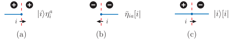
Figure 11: Rules for index lines crossing a cut leg $i$ carrying momentum $p_{i}$. If both sides of the cut are (a) MHV or both are (b) $\overline{\hbox{MHV}}$ then the index line ends at the cut. This is equivalent to the insertion of a super-momentum $|i\rangle\eta^{a}_{i}$ in the MHV case, or conjugate super-momentum $\widetilde{\eta}_{ia}[i|$ in the $\overline{\hbox{MHV}}$ case. If one side is MHV and the other $\overline{\hbox{MHV}}$ then the index line is continuous across the cut and corresponds to the insertion of $|i\rangle\eta^{a}_{i}\widetilde{\eta}_{ia}[i|$, or as illustrated, the insertion of the cut momentum $|i\rangle[i|$, as discussed in section V.3. Dashed (red) lines mark cuts, solid (blue) denote $SU(4)$ index lines, and plus or minus labels denote whether an amplitude on a given side of a cut is MHV or $\overline{\hbox{MHV}}$. The arrows indicate the momentum direction.

Having defined the mixed superspace state sum, let us consider the actions of the three types of sewing operators. We note that the only objects in the product ${\cal A}_{L}{\cal A}_{R}$ that survive the supersum integrations of eq. (68), for leg $i$ and index $a$, are those terms proportional to,

$${\rm(a)}:\;\;|i\rangle\eta_{i}^{a}=q^{a}_{i}\,,$$

$${\rm(b)}:\;\;\widetilde{\eta}_{ia}[i|=\tilde{q}_{ia}\,,$$

$${\rm(c)}:\;\;|i\rangle\eta_{i}^{a}\widetilde{\eta}_{ia}[i|\hskip 5.69054pt{\rm or}\hskip 5.69054pt1\,,$$ (71)

where (a), (b) and (c) refers to the aforementioned cases, and where the “1” in case (c) denotes an absence of both $\widetilde{\eta}_{ia}$ and $\eta_{i}^{a}$. Furthermore, we note that since $\hat{I}^{a}_{i,\,+-}$ is a Grassmann even operator we can immediately carry out the integration of case (c),

$${\rm(c)}:\;\;|i\rangle[i|=p_{i}\hskip 5.69054pt{\rm or}\hskip 5.69054pt1\,.$$ (72)

However this has to be done with some care, as will be discussed in section section V.3.2, where a precise rule will be given.

Interpreting the supermomenta of eq. (71) and momenta of eq. (72) as parts of $SU(4)$ index lines, gives us the pictorial rules displayed in fig. 11 for the transition condition of an index line across a cut. For an MHV-MHV transition the index line ends (or starts) at the cut, corresponding to the insertion of a supermomentum $|i\rangle\eta_{i}^{a}$. Similarly, for an $\overline{\hbox{MHV}}$-$\overline{\hbox{MHV}}$ transition, the index line ends (or starts) at the cut, corresponding to the insertion of a conjugate supermomentum $\widetilde{\eta}_{ia}[i|$. In contrast, for an MHV-$\overline{\hbox{MHV}}$ transition, the index lines are continuous across a cut.” This can happen in two ways, either the two lines on each side meet at the cut, or there are no index line on leg $i$ on either side of the cut. The latter option corresponds to the trivial insertion of a unit factor. The former option can be interpreted as either an insertion of a product between a supermomentum and its conjugate $|i\rangle\eta_{i}^{a}\widetilde{\eta}_{ia}[i|$ as in eq. (71)(c), or it can be interpreted as an insertion of momentum $|i\rangle[i|$ according to eq. (72), as is displayed in fig. 11(c). These two interpretations will give rise to two different sets of rules for carrying out the supersum (see section V.3). In both cases the $SU(4)$ index-line diagrams will be identical.

V.2 One-loop warm-up

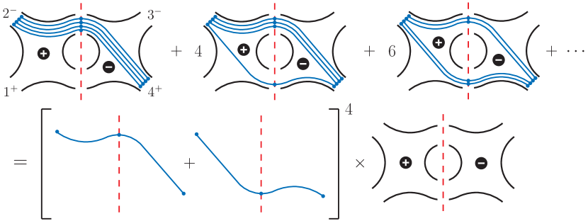
Figure 12: A unitarity cut of the four-gluon amplitude $A^{\rm 1\hbox{-}loop}_{4}(1^{+},2^{-},3^{-},4^{+})$, involving one MHV and one $\overline{\hbox{MHV}}$ superamplitude. The top-left diagram represents a gluon loop, the top-central diagram represents the four contributions in a fermion loop, and the top-right diagram represents the six scalar state contributions. The ellipsis denote that four more fermion-loop and one more gluon-loop contributions are suppressed. The bottom diagram illustrates that the 16 contributions may be resummed, and that each index line may be treated independently. The circle in each diagram is a one-loop “hole” and the dashed line marks the cut. The fourth power over the index lines should be interpreted as a product over the four $SU(4)$ indices.

We start with a simple one-loop example to pictorially illustrate the state sum of a ${{\cal N}=4}$ cut. We will postpone the analytic evaluation of index diagrams to the following section.

Consider the one-loop cut of fig. 12. Reading off the index lines that end on external legs, this cut corresponds to the purely gluonic amplitude $A^{\rm 1\hbox{-}loop}_{4}(1^{+},2^{-},3^{-},4^{+})$. The left side of the cut is chosen to be MHV and right side is $\overline{\hbox{MHV}}$, which means that the $SU(4)$ index lines must be continuous through the cut. The different diagrams in the top of fig. 12 correspond to the different states in the ${{\cal N}=4}$ gauge supermultiplet. There are five such diagrams although only three are shown, the two hidden in the ellipsis are horizontal flips of the first two shown. The combinatoric factors in front of each diagram are the distinct ways of obtaining the same diagram, tracking of the $SU(4)$ labels. As shown in the figure, the sum over the diagrams can be interpreted as a product over the four SU(4) indices, depicted as a fourth power. This is consistent with the general result discussed in section IV: summing over the states crossing a cut composed of a product of MHV and $\overline{\hbox{MHV}}$ tree amplitudes is a sum of terms raised to the fourth power. In the diagrammatic language of index lines this also leads to the simplification which allows us to consider each of the four $SU(4)$ index-line factors independently. Thus in the remaining part of this paper all index diagrams will be drawn for only a single $SU(4)$ index.

Interestingly, the index diagrams follow a “sum over paths” principle analogous to the one of quantum mechanics. In our one-loop example, a single continuous index line has two possible allowed paths, crossing the cut through either the upper or lower internal leg. Thus, there are two terms for each index in the state sum or a total of $2^{4}$ for the four index lines. For cuts which factorize into adjacent MHV amplitudes or adjacent $\overline{\hbox{MHV}}$ amplitudes, the index lines are discontinuous, or the “paths” are broken into several pieces, as explained in the previous section. See the following sections for explicit examples of this.

More generally, for external gluon amplitudes the structure discussed in the above one-loop example is quite generic for any configuration of MHV and $\overline{\hbox{MHV}}$ tree amplitudes appearing in a cut. With external gluons the four $SU(4)$ index lines all start on the same legs, allowing us to treat each of the lines identically. If some of the external particles are scalars or fermions then the $SU(4)$ index lines can start at different external legs, but in any case, each of the four $SU(4)$ index lines can be treated independently. As discussed in section II, if a non-MHV tree amplitude appears we simply insert its expansion in terms of MHV or $\overline{\hbox{MHV}}$ amplitudes into the cut, effectively reducing the evaluation of the relevant supersums to the discussion above.

V.3 Rules for converting diagrams to spinor expressions

As explained in section II.3, each index line drawn for an MHV tree amplitude (in a cut) corresponds to a factor $\left\langle q^{a}_{i}\,q^{a}_{j}\right\rangle$, and for an $\overline{\hbox{MHV}}$ tree amplitude it corresponds to a factor $\left[\tilde{q}_{ia}\,\tilde{q}_{ja}\right]$. Since both $\left\langle q_{i}^{a}\,q_{j}^{a}\right\rangle$ and $\left[\tilde{q}_{ia}\,\tilde{q}_{ja}\right]$ are Grassmann even as well as symmetric under the exchange $i\leftrightarrow j$ it may seem to be a straightforward task to convert the index diagrams to analytic expressions. However, in practice there are different strategies for converting the Grassmann-valued numerators to spinor expressions, two of which we describe here. First we note that since the index diagrams have pre-selected the terms that survive in the supersum, the application of any supersum operator on an index diagram serves only to convert the product of $\eta$’s and $\widetilde{\eta}$’s to a $\pm 1$ factor, which can be achieved by simple replacements rules. The two alternative replacement rules are:

V.3.1 Rule 1: Sign assignment in $\eta$-only superspace

One option, which will avoid the slightly more complicated MHV-$\overline{\hbox{MHV}}$ transition operator $\hat{I}^{a}_{i,\,+-}$, is to make use of the Fourier transform and work only in $\eta$ superspace. (It also does not require the $\widetilde{\eta}$ sign flip for incoming momenta given in eq. (70).) We Fourier transform all the $\left[\tilde{q}_{ia}\,\tilde{q}_{ja}\right]$ factors according to the rule in eq. (16),

$$\left[\tilde{q}_{ia}\,\tilde{q}_{ja}\right]\stackrel{{\scriptstyle\widehat{F}}}{{\longrightarrow}}\eta_{1}^{a}\cdots\eta_{i-1}^{a}\,[i|\,\eta_{i+1}^{a}\cdots\eta_{j-1}^{a}\,|j]\,\eta_{j+1}^{a}\cdots\eta_{m}^{a}\,,$$ (73)

where $1,\ldots,m$ are the legs of the particular $\overline{\hbox{MHV}}$ amplitude that the $\left[\tilde{q}_{ia}\,\tilde{q}_{ja}\right]$ factor belongs to. Recall that in this rule the positions of $[i|$ and $|j]$ count giving additional signs as they are pushed past the $\eta$’s. Also note that for an odd number of legs $m$ the Fourier transform maps the Grassmann even object $\left[\tilde{q}_{ia}\,\tilde{q}_{ja}\right]$ to a Grassmann odd object, thus care has to be taken to not alter the position of $\left[\tilde{q}_{ia}\,\tilde{q}_{ja}\right]$ relative to the position of, say, $\left[\tilde{q}_{ib}\,\tilde{q}_{jb}\right]$ in the cut expression.

After the Fourier transform, every term in the cut will contain exactly the same product of $\eta$’s, albeit in different orderings. For each term and each $SU(4)$ index this product can be converted to a $\pm$ sign by the replacement,

$$\eta^{a}_{i_{1}}\eta^{a}_{i_{2}}\cdots\eta^{a}_{i_{n-1}}\eta^{a}_{i_{n}}\rightarrow{\rm signature}[i_{1}i_{2}\cdots i_{n-1}i_{n}]\,,$$ (74)

where the signature function gives the signature of the permutation of the legs relative to a canonical ordering, and here $n$ is the number of internal legs plus the number of the external $\eta$’s. This rule is particularly easy to automate.

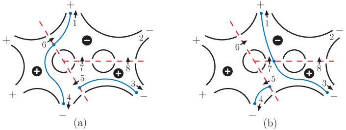
Figure 13: Examples of contributions to a unitarity cut of a six-point two-loop NMHV amplitude drawn as index-line diagrams for a single $SU(4)$ index. Two routings (a) and (b) of the index lines are shown; routing (c) referred to in the main text is similar to (b), but where the longer index line, attached to legs 1 and 3, passes through cut leg 8 rather than cut leg 7. Note that only legs necessary for the subsequent discussion are labeled.

We will illustrate this rule by an example. Consider the index diagrams in fig. 13, which correspond to a particular contribution to a two-loop cut with gluonic external states. For a single $SU(4)$ index there are three contributions (a), (b) and (c), two of which are shown. Reading off the numerator factors from the shaded (blue) index lines we have

$${\rm(a)}: \;\;(\eta_{4}\left\langle 4\,6\right\rangle\eta_{6})(\eta_{3}\left\langle 3\,5\right\rangle\eta_{5})([1|\eta_{2}|6]\eta_{7}\eta_{8})\;\,\rightarrow\left\langle 4\,6\right\rangle\left\langle 3\,5\right\rangle\left[1\,6\right]\,,$$ (75)

$${\rm(b)}: \;\;(\eta_{5}\langle-5\,4\rangle\eta_{4})(\eta_{7}\left\langle 7\,3\right\rangle\eta_{3})([1|\eta_{2}\eta_{6}|7]\eta_{8})\rightarrow\left\langle 5\,4\right\rangle\left\langle 7\,3\right\rangle\left[1\,7\right]\,,$$

$${\rm(c)}: \;\;(\eta_{5}\langle-5\,4\rangle\eta_{4})(\eta_{8}\left\langle 8\,3\right\rangle\eta_{3})([1|\eta_{2}\eta_{6}\eta_{7}|8])\rightarrow\left\langle 5\,4\right\rangle\left\langle 8\,3\right\rangle\left[1\,8\right]\,,$$

where we have suppressed the $SU(4)$ index since we consider only a single component. To get to the right-hand-side we first rearrange the $\eta$’s using the rule (16) that the spinors anticommute with the $\eta$’s, and then remove them after arranging them into a chosen canonical order $\eta_{2}\eta_{3}\eta_{4}\eta_{5}\eta_{6}\eta_{7}\eta_{8}$. Leg 5 also carries a negative sign since it is an incoming label in (b) and (c), this sign must be properly extracted following eq. (7). For external gluons each of the four $SU(4)$ indices give identical results, leading to the following numerator factor for the cut contribution:

$$\Bigl{(}\left\langle 4\,6\right\rangle\left\langle 3\,5\right\rangle\left[1\,6\right]+\left\langle 5\,4\right\rangle\left\langle 7\,3\right\rangle\left[1\,7\right]+\left\langle 5\,4\right\rangle\left\langle 8\,3\right\rangle\left[1\,8\right]\Bigr{)}^{4}\,.$$ (76)

V.3.2 Rule 2: Sign assignment in a mixed $\eta$-$\widetilde{\eta}$ superspace

Alternatively, we can construct a rule that treats $\eta$ and $\widetilde{\eta}$ on equal footing. With this rule we must strictly impose the sign rule eq. (70) that flips the sign of $\widetilde{\eta}_{i}$ as well as conjugate supermomenta $\tilde{q}_{i}$ under momentum direction flips $i\rightarrow-i$. The mixed-superspace sign rules are based on the observation in section V.1 that the MHV-$\overline{\hbox{MHV}}$ transition operator $\widehat{I}^{a}_{i,\,+-}$ can be immediately applied to the cut to remove all Grassmann parameters associated with internal lines on the border between MHV and $\overline{\hbox{MHV}}$ amplitudes. However, it must be done with some care, as is easily illustrated by an example. Consider the two ways of removing the $\eta_{i}^{a}\widetilde{\eta}_{ia}$ factor,

$$\left\langle q^{a}_{j}\,q^{a}_{i}\right\rangle\left[\tilde{q}_{ia}\,\tilde{q}_{ka}\right]\rightarrow\eta_{j}^{a}\left\langle j\,i\right\rangle\left[i\,k\right]\widetilde{\eta}_{ka}\,,$$

$$\left[\tilde{q}_{ka}\,\tilde{q}_{ia}\right]\left\langle q_{i}^{a}\,q_{j}^{a}\right\rangle\rightarrow\widetilde{\eta}_{ka}\left[k\,i\right]\left\langle i\,j\right\rangle\eta^{a}_{j}\,.$$ (77)

The two left-hand sides are clearly equal, but the two right-hand would differ by signs since $\eta^{a}_{j}$ anticommute with $\widetilde{\eta}_{ka}$. However, if we instead think of $\eta$’s and $\widetilde{\eta}$’s as living in two different mutually commuting Grassmann spaces then the sign inconsistency in eq. (77) is resolved. Although unconventional, this construction gives us a consistent treatment of the sign of the index-line contributions. We will not go further into the details of proving that this assertion is valid. Instead we will state the final rules.

The rules that convert the index lines to spinor products, while treating $\eta$ and $\widetilde{\eta}$ on equal footing are: For each unbroken index line, write down the corresponding spinor string (using momenta) following either direction of the line. Multiply with appropriate Grassmann odd parameters at the endpoints of the line, as shown in fig. 11. Use the sign rules of eq. (7) and eq. (70) to deal with the case of incoming momenta (or supermomenta). Now since each term in the cut has exactly the same index-line endpoints (due to the spinor weight carried by these points), every term will be multiplied by the same product of $\eta$’s and $\widetilde{\eta}$’s, albeit in different orderings. The sign map for each term is then,

$$\eta^{a}_{i_{1}}\eta^{a}_{i_{2}}\cdots\eta^{a}_{i_{l}}\;\widetilde{\eta}_{j_{1}a}\widetilde{\eta}_{j_{2}a}\cdots\widetilde{\eta}_{j_{m}a}\rightarrow{\rm signature}[i_{1}i_{2}\cdots i_{l}]\,{\rm signature}[j_{1}j_{2}\cdots j_{m}]\,,$$ (78)

where the $\eta$’s commute with the $\widetilde{\eta}$’s, $l$ is the number of legs on an MHV-MHV border plus number of external $\eta$’s, and $m$ is the number of legs at an $\overline{\hbox{MHV}}$- $\overline{\hbox{MHV}}$ border plus the number of external $\widetilde{\eta}$’s.

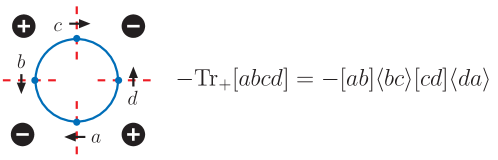
Figure 14: According to the mixed superspace sign rules (“rule 2”) a closed loop of index lines corresponds to a (chiral) trace of only momenta, no supermomenta, with an explicit insertion of a negative sign, reflecting the fermionic nature of index lines. (For clarity the momenta are here directed so that no implicit sign comes out of the spinors according to the sign rules eq. (7).)

An important special case is if the index lines form a closed loop. Then there are no Grassmann parameters present, only spinors enter, or momenta in the form of a chiral trace, as shown in fig. 14. The proper prescription for this case is to insert an explicit factor $(-1)$ for each closed index loop. This corresponds to the standard prescription for fermion loops, and thus it reflects the fermionic nature of the index lines.

To see how the mixed superspace works consider again the example in fig. 13. We read off the diagrams, giving,

$${\rm(a)}: \;\;(\widetilde{\eta}_{1}[1|6|4\rangle\eta_{4})(\eta_{3}\left\langle 3\,5\right\rangle\eta_{5})~{}~{}\rightarrow-[1|6|4\rangle\left\langle 3\,5\right\rangle\,,$$ (79)

$${\rm(b)}: \;\;(\widetilde{\eta}_{1}[1|7|3\rangle\eta_{3})(\eta_{5}\langle-5\,4\rangle\eta_{4})\,\rightarrow~{}\,~{}[1|7|3\rangle\left\langle 5\,4\right\rangle\,,$$

$${\rm(c)}: \;\;(\widetilde{\eta}_{1}[1|8|3\rangle\eta_{3})(\eta_{5}\langle-5\,4\rangle\eta_{4})\,\rightarrow~{}\,~{}[1|8|3\rangle\left\langle 5\,4\right\rangle\,.$$

where $[i|j|k\rangle\equiv\left\langle i\,j\right\rangle\left[j\,k\right]$. As discussed above, we commute the $\widetilde{\eta}$ past the $\eta$’s, and place them in the canonical order $\eta_{3}\eta_{4}\eta_{5}\widetilde{\eta}_{1}$, after which they are removed. The result is equivalent to the first rule, but perhaps is simpler to carry out manually.

V.4 Supersum simplifications

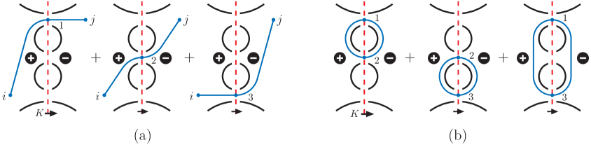
Figure 15: Two examples of momentum conservation identities, allowing us to convert loop momenta to external momenta. In (a) we have three index lines that can be summed up to $\eta_{i}\langle i|l_{1}+l_{2}+l_{3}|j]\widetilde{\eta}_{j}$. Because the vertical cut cross the entire diagram the sum of loop momenta can be re-expressed in terms of external momentum $K=l_{1}+l_{2}+l_{3}$ . Similarly, for (b) the sum over index lines give $-2l_{1}\cdot l_{2}-2l_{2}\cdot l_{3}-2l_{1}\cdot l_{3}=-K^{2}$.

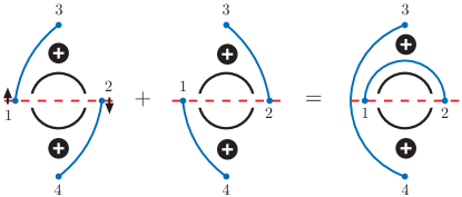
Figure 16: A pictorial representation of Schouten’s identity. All index lines carry the same suppressed $SU(4)$ index. (Note that the supermomentum $q_{i}$ flips sign according to eq. (7) depending on which side of the dashed (red) cut line the shaded (blue) index line extends.)

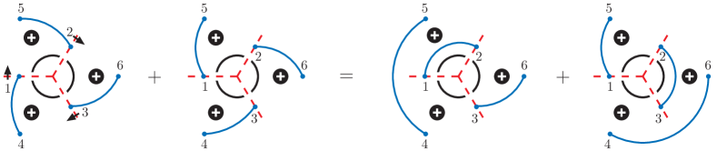
Figure 17: Pictorial representation of more complicated applications of Schouten’s identity.

In contrast to the algebraic approach of section IV, the index-diagram approach typically gives results that may be further simplified. In particular, in order to fully expose cancellations of powers of loop momenta due to supersymmetry, rearrangements using momentum conservation and Schouten’s identity are generally necessary. Two typical situations where momentum conservation allows us to pull out powers of loop momenta as external momenta are displayed in fig. 15. Using the mixed-superspace rules (rule 2), the index lines correspond to,

$${\rm(a)}:\;\;\eta_{i}\langle i|l_{1}|j]\widetilde{\eta}_{j}+\eta_{i}\langle i|l_{2}|j]\widetilde{\eta}_{j}+\eta_{i}\langle i|l_{3}|j]\widetilde{\eta}_{j}=\eta_{i}\langle i|l_{1}+l_{2}+l_{3}|j]\widetilde{\eta}_{j}\,,$$

$${\rm(b)}:\;\;-\left\langle l_{1}\,l_{2}\right\rangle\left[l_{2}\,l_{1}\right]-\left\langle l_{2}\,l_{3}\right\rangle\left[l_{3}\,l_{2}\right]-\left\langle l_{1}\,l_{3}\right\rangle\left[l_{3}\,l_{1}\right]=-(l_{1}+l_{2}+l_{3})^{2}\,,$$ (80)

where the $R$-symmetry indices have been suppressed, and where the negative signs are due to the rule of fig. 14 for closed index line loops. In both cases we have a vertical cut which runs from one side of a diagram to the other, therefore the loop momentum sum corresponds to the external momentum $K=l_{1}+l_{2}+l_{3}$ crossing the cut, by momentum conservation.

Another important manipulation follows from Schouten’s identity displayed pictorially in fig. 16. Reading off the index diagrams we have,

$$\left\langle-q_{1}\,q_{3}\right\rangle\left\langle-q_{2}\,q_{4}\right\rangle+\left\langle q_{1}\,q_{4}\right\rangle\left\langle q_{2}\,q_{3}\right\rangle=\left\langle-q_{1}\,q_{2}\right\rangle\left\langle q_{3}\,q_{4}\right\rangle\,,$$ (81)

in terms of supermomentum spinor products (20). This can be written in a symmetric form. Extracting the signs from the incoming supermomenta (7) gives,

$$\left\langle q_{1}\,q_{3}\right\rangle\left\langle q_{2}\,q_{4}\right\rangle+\left\langle q_{1}\,q_{4}\right\rangle\left\langle q_{2}\,q_{3}\right\rangle+\left\langle q_{1}\,q_{2}\right\rangle\left\langle q_{3}\,q_{4}\right\rangle=0\,,$$ (82)

which expresses Schouten’s identity as the statement that $\left\langle q_{1}\,q_{2}\right\rangle\left\langle q_{3}\,q_{4}\right\rangle$ symmetrized over all legs vanishes. (From this it also follows that all spinor strings involving $2n>2$ super-momenta vanish upon symmetrization.) In terms of regular bosonic spinor products, this is equivalent to the usual Schouten’s identity where the anti-symmetrization of the spinor strings vanishes. We note that although the orginal index lines start and end on legs within a single tree amplitudes, after an application of Schouten’s identity in fig. 16, they can begin and end on legs of different tree amplitudes in the cuts.

Besides the basic identity more complicated versions may be needed. For example, for the configuration in fig. 17, we have the identity,

$$\left\langle q_{1}\,q_{4}\right\rangle\left\langle q_{2}\,q_{5}\right\rangle\left\langle q_{3}\,q_{6}\right\rangle+\left\langle-q_{1}\,q_{5}\right\rangle\left\langle-q_{2}\,q_{6}\right\rangle\left\langle-q_{3}\,q_{4}\right\rangle$$

$$\hskip 113.81102pt=\left\langle q_{4}\,q_{5}\right\rangle\left\langle-q_{1}\,q_{2}\right\rangle\left\langle q_{3}\,q_{6}\right\rangle+\left\langle-q_{1}\,q_{5}\right\rangle\left\langle q_{4}\,q_{6}\right\rangle\left\langle-q_{2}\,q_{3}\right\rangle\,,\hskip 14.22636pt$$ (83)

which is obtained by a composition of two applications of Schouten’s identity.

We note that the identities presented in this section remains valid under conjugation: $\langle\rangle\leftrightarrow[]$, $q\leftrightarrow\tilde{q}$, $\eta\leftrightarrow\widetilde{\eta}$, MHV $\leftrightarrow$ $\overline{\hbox{MHV}}$.

V.5 Three-loop examples

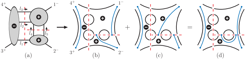
Figure 18: A contribution of a three-loop cut (a) in terms of index diagrams tracking only a single $SU(4)$ index (b) and (c). Diagram (d) follows from applying Schouten’s identity given in fig. 16 to (b) and (c). The index lines in diagrams (b) and (c) all begin and end on legs of the same tree amplitude, but as in diagram (d), after application of Schouten’s identity, an index line can connect legs of different tree amplitudes. The other independent configuration of holomorphicity of the tree amplitudes for this cut is given in fig. 19.

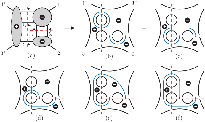
Figure 19: The same cut topology as in fig. 18, but for the other independent configuration of tree amplitudes.

To illustrate the use of the index diagrams in a non-trivial example consider the cut of the three-loop four-point amplitude shown in figs. 18(a) and 19(a) in terms of MHV and $\overline{\hbox{MHV}}$ tree amplitudes. We have taken the external legs to be gluons with helicity assignments $(1^{-},2^{-},3^{+},4^{+})$ allowing all possible states of the ${{\cal N}=4}$ theory to circulate in the loops. In this case there are two distinct configurations of MHV and $\overline{\hbox{MHV}}$ tree amplitudes in the cuts separated into the two figures. As mentioned in section II.3, the four-point trees can be chosen to be either holomorphic or anti-holomorphic, so flipping the identification of four-point trees from MHV to $\overline{\hbox{MHV}}$ does not lead to distinct contributions.

Consider first the configuration in fig. 18, where two of the tree amplitudes composing the cut are MHV and one is $\overline{\hbox{MHV}}$. We have,

$$\hskip-40.0ptC^{\rm fig.\;\ref{ThreeLoopPlanarExample_aFigure}}=\sum_{\rm states}A_{5}^{\rm\overline{MHV}}(3^{+},4^{+},l_{3},l_{2},l_{1})\,A_{5}^{\rm MHV}(1^{-},-l_{5},-l_{4},-l_{2},-l_{3})\,A_{4}^{\rm MHV}(2^{-},-l_{1},l_{4},l_{5})\hskip 8.5359pt$$

$$= i\rho^{\rm fig.\;\ref{ThreeLoopPlanarExample_aFigure}}{1\over\left[3\,4\right]\left[4\,l_{3}\right]\left[l_{3}\,l_{2}\right]\left[l_{2}\,l_{1}\right]\left[l_{1}\,3\right]}\,{1\over\left\langle 1\,l_{5}\right\rangle\left\langle l_{5}\,l_{4}\right\rangle\left\langle l_{4}\,l_{2}\right\rangle\left\langle l_{2}\,l_{3}\right\rangle\left\langle l_{3}\,1\right\rangle}\,{1\over\left\langle 2\,l_{1}\right\rangle\left\langle l_{1}\,l_{4}\right\rangle\left\langle l_{4}\,l_{5}\right\rangle\left\langle l_{5}\,2\right\rangle}\,,$$

where the numerator result of the supersum contained in $\rho^{\rm fig.\;\ref{ThreeLoopPlanarExample_aFigure}}$ can be obtained from the index diagrams in fig. 18. The routings (b) and (c) are the only possibilities for a single $SU(4)$ index. This can be worked out following the rules that index lines, corresponding to physical states, are discontinuous between two MHV amplitudes and continuous between MHV and $\overline{\hbox{MHV}}$ amplitudes. Furthermore, every MHV and $\overline{\hbox{MHV}}$ tree amplitude contains exactly one index line per $SU(4)$ index. Each line must properly attach to the external assignment of $SU(4)$ indices (in this case the helicity of the external gluons). Using either set of rules for reading the diagrams in section V.3 gives the single-index-line numerator,

$$-\left[\tilde{q}_{3}\,\tilde{q}_{4}\right]\left\langle q_{l_{4}}\,q_{2}\right\rangle\left\langle q_{1}\,q_{l_{5}}\right\rangle-\left[\tilde{q}_{3}\,\tilde{q}_{4}\right]\left\langle q_{l_{5}}\,q_{2}\right\rangle\left\langle q_{1}\,q_{l_{4}}\right\rangle=\left[\tilde{q}_{3}\,\tilde{q}_{4}\right]\left\langle q_{1}\,q_{2}\right\rangle\left\langle q_{l_{4}}\,q_{l_{5}}\right\rangle\,.$$ (85)

The right-hand side corresponds to fig. 18(d) which is obtained from fig. 18(b) and (c) after applying the pictorial Schouten’s identity in fig. 16. Dropping the Grassmann parameters and raising the result to fourth power immediately yields,

$$\rho^{\rm fig.\;\ref{ThreeLoopPlanarExample_aFigure}}=\left[3\,4\right]^{4}\left\langle 1\,2\right\rangle^{4}\left\langle l_{4}\,l_{5}\right\rangle^{4}\,.$$ (86)

The other distinct contribution of holomorphicity of tree amplitudes in fig. 19, while somewhat more complicated, is quite similar. For this contribution we have,

$$C^{\rm fig.\;\ref{ThreeLoopPlanarExample_bFigure}} \!=\! \sum_{\rm states}A_{5}^{\rm MHV}(3^{+},4^{+},l_{3},l_{2},l_{1})\,A_{5}^{\rm\overline{MHV}}(1^{-},-l_{5},-l_{4},-l_{2},-l_{3})\,A_{4}^{\rm\overline{MHV}}(2^{-},-l_{1},l_{4},l_{5})$$

$$= \!i\rho^{\rm fig.\;\ref{ThreeLoopPlanarExample_bFigure}}{1\over\left\langle 3\,4\right\rangle\left\langle 4\,l_{3}\right\rangle\left\langle l_{3}\,l_{2}\right\rangle\left\langle l_{2}\,l_{1}\right\rangle\left\langle l_{1}\,3\right\rangle}\,{1\over\left[1\,l_{5}\right]\left[l_{5}\,l_{4}\right]\left[l_{4}\,l_{2}\right]\left[l_{2}\,l_{3}\right]\left[l_{3}\,1\right]}\,{1\over\left[2\,l_{1}\right]\left[l_{1}\,l_{4}\right]\left[l_{4}\,l_{5}\right]\left[l_{5}\,2\right]}\,.$$

The result of the state sum is contained in the factor $\rho^{\rm fig.\;\ref{ThreeLoopPlanarExample_bFigure}}$ and can be read off from the index lines in fig. 19. Using the mixed superspace rules (rule 2), the five diagrams in this figure (b)-(f) yield a numerator factor,

$$-\left\langle l_{2}\,l_{3}\right\rangle\left[l_{3}\,l_{2}\right]\left[\tilde{q}_{l_{4}}\,\tilde{q}_{l_{5}}\right]-\widetilde{\eta}_{l_{4}}[l_{4}|l_{1}l_{2}|l_{5}]\widetilde{\eta}_{l_{5}}-\widetilde{\eta}_{l_{4}}[l_{4}|l_{2}l_{1}|l_{5}]\widetilde{\eta}_{l_{5}}-\widetilde{\eta}_{l_{4}}[l_{4}|l_{1}l_{3}|l_{5}]\widetilde{\eta}_{l_{5}}-\widetilde{\eta}_{l_{4}}[l_{4}|l_{3}l_{1}|l_{5}]\widetilde{\eta}_{l_{5}}$$

$$\hskip 56.9055pt=-(\left\langle l_{2}\,l_{3}\right\rangle\left[l_{3}\,l_{2}\right]+\left\langle l_{1}\,l_{2}\right\rangle\left[l_{2}\,l_{1}\right]+\left\langle l_{1}\,l_{3}\right\rangle\left[l_{3}\,l_{1}\right])\left[\tilde{q}_{l_{4}}\,\tilde{q}_{l_{5}}\right]$$

$$\hskip 56.9055pt=-(l_{1}+l_{2}+l_{3})^{2}\left[\tilde{q}_{l_{4}}\,\tilde{q}_{l_{5}}\right]$$

$$\hskip 56.9055pt=-s\left[\tilde{q}_{l_{4}}\,\tilde{q}_{l_{5}}\right]\,.$$ (88)

The second line in this equation is obtained by applying the pictorial Schouten’s identity displayed in fig. 16 to the second and third contributions in fig. 19, as well as to the fourth and fifth. This gives the second line corresponding to the diagrams displayed in fig. 20. The result on the last line of eq. (88) follows from momentum conservation $(l_{1}+l_{2}+l_{3})^{2}=(k_{1}+k_{2})^{2}=s$. Stripping the anticommuting parameters and raising the result to the fourth power gives us the desired numerator,

$$\rho^{\rm fig.\;\ref{ThreeLoopPlanarExample_bFigure}}=s^{4}\left[l_{4}\,l_{5}\right]^{4}\,.$$ (89)

This displays a cancellation of a total of eight powers of loop momenta from the numerator of the cut.

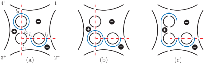
Figure 20: Simplified results after applying Schouten’s identity. Diagram (a) is just diagram (b) of fig. 19, while diagram (b) is obtained by combining diagrams (c) and (d) of fig. 19 via the pictorial Schouten’s identity in fig. 16. Similarly, diagram (c) comes from combining diagrams (e) and (f) of fig. 19. This form exposes supersymmetric cancellation, allowing us to extract factors depending only on external momenta from each cut numerator.

Rather remarkably, we see that after dividing out the four-point tree amplitude, the two contributions (86) and (88) corresponding to figs. 18 and 19 are complex conjugates of each other

$$\frac{C^{\rm fig.\;\ref{ThreeLoopPlanarExample_bFigure}\rm(b)}}{A^{\rm tree}_{4}}=\Biggl{(}\frac{C^{\rm fig.\;\ref{ThreeLoopPlanarExample_aFigure}\rm(a)}}{A^{\rm tree}_{4}}\Biggr{)}^{*}\,.$$ (90)

The tree amplitude in this equation is given (see eq. (4)) by,

$$A_{4}^{\rm tree}(1^{-},2^{-},3^{+},4^{+})=i\frac{\left\langle 1\,2\right\rangle^{4}}{\left\langle 1\,2\right\rangle\left\langle 2\,3\right\rangle\left\langle 3\,4\right\rangle\left\langle 4\,1\right\rangle}=i\frac{\left[3\,4\right]^{4}}{\left[1\,2\right]\left[2\,3\right]\left[3\,4\right]\left[4\,1\right]}\,.$$ (91)

which are the MHV and $\overline{\hbox{MHV}}$ forms of the four-gluon amplitude. To make the relation (90) manifest, on the left side we use the MHV form of the tree amplitude while on the right side we use the $\overline{\hbox{MHV}}$ form. Thus, after removing an overall factor of the tree amplitude the two contributions add up to a real expression. A consequence of this observation is that the cut can be expressed entirely in terms of scalar products of momenta multiplied by an overall factor of the tree amplitude. (Terms containing the Levi-Civita tensor cancel.) For amplitudes other than four-point ones, this property no longer holds Fusing .

VI Tracking Contributions

The $R$-symmetry index-diagram approach allows us to track the contributions of individual states in four-dimensional cuts. This observation has some interesting consequences. In particular, as we outline below, we can give rules for constructing cuts of amplitudes in various theories with fewer supersymmetries. We also use this observation to obtain rules for finding the contributions of the complete ${{\cal N}=4}$ supermultiplet starting from the easily enumerated purely gluonic contributions. We illustrate this with some non-trivial four-loop examples, relevant to the construction of the complete four-loop four-point amplitude of the ${{\cal N}=4}$ theory FourLoopNonPlanar .

VI.1 Cases with fewer supersymmetries

Certain theories with reduced supersymmetry may be constructed simply by truncating the spectrum of the ${{\cal N}=4}$ theory. As discussed in section V the supersums contributing to cuts of amplitudes with external gluons are always the fourth power of a sum of terms

$$(A+B+C+\dots)^{\cal N}\,,\hskip 28.45274pt{{\cal N}=4}\,,$$ (92)

where the summands $A,B,C,\dots$ represent the possible spinorial numerator factors encoded by the $SU(4)$ index diagrams. They correspond to the possible paths, or routings, of an index line, after all $\eta$’s and $\widetilde{\eta}$’s have been removed. After expanding (92), the terms are in one-to-one correspondence to individual particles and helicity configurations. In particular, index lines routed in groups of four correspond to purely-gluonic states and give the numerator terms $A^{4},B^{4},C^{4}\dots$—a fact which we exploit below in section VI.2. Combinations where the four index lines follow different routings give rise to the cross terms in the product (92). These terms correspond to cases where scalar and fermion fields of the supermultiplet propagate, e.g. terms such as $A^{3}B$ or $A^{2}B^{2}$ arise from fermion and scalar states in the loops (see fig. 12 for explicit examples). Precise tracking of the matter fields through the cuts is dictated by the index-line diagrams.

For a few theories which are closely related to ${{\cal N}=4}$ super-Yang-Mills theory it is possible to write down closed form expressions for the cuts of their scattering amplitudes in terms of the ${{\cal N}=4}$ cuts. This is a consequence of the fact that the ${\cal N}=4$ vector multiplet decomposes in a direct sum of representations of ${\cal N}<4$ supersymmetry algebras. By systematically dropping contributions following their $R$-charges, we obtain cuts of amplitudes in theories with reduces supersymmetry and a field content which is a subset of that of ${{\cal N}=4}$ SYM.

Starting from the ${{\cal N}=4}$ spectrum we may eliminate one ${\cal N}=2$ hypermultiplet to obtain the spectrum of the pure ${\cal N}=2$ super-Yang-Mills theory. This can be done by expressing the representations of the $SU(4)$ $R$-symmetry in representations of an $SU(2)\times SU(2)\times U(1)$ subgroup and restricting to states transforming trivially under one $SU(2)$ factor. Without loss of generality, this may be taken to act on indices 3 and 4; this truncation breaks $SU(4)$ down to $SU(2)$, giving the following states:

$$g_{+}\,,\hskip 42.67912ptf_{+}^{a}\,,\hskip 42.67912pts^{ab}\,,\hskip 42.67912pts^{34}\,,\hskip 42.67912ptf^{b34}_{-}\,,\hskip 42.67912ptg_{-}^{ab34}\,;$$ (93)

here $a,b=1$ or $2$ are the $SU(2)$ $R$-symmetry indices. Although indices 3 and 4 no longer plays the role of group indices, we keep them as labels to distinguish the states and to keep notation uniform with the ${{\cal N}=4}$ case. As expected, there are two fermions which, on-shell, correspond to four states $f_{+}^{a}$ and $f^{b34}_{-}$. The two scalar fields are complex conjugates $(s^{34})^{*}=s^{12}$, thus the counting of on-shell states is consistent with the ${\cal N}=2$ gauge multiplet.

In terms of the index diagrams this truncation implies that we should keep only those diagrams where indices 3 and 4 are grouped together. For external gluons, this gives the following cut numerator,

$$(A+B+C+\dots)^{2}(A^{2}+B^{2}+C^{2}+\dots)\,,$$ (94)

where $A,B,C$ represent the same terms as in eq. (92), and the squares $A^{2},B^{2},C^{2}$ are a consequence of the above requirement that two indices are always grouped together in the diagrams.

In the same spirit, by dropping one chiral multiplet from the ${\cal N}=2$ spectrum we obtain the on-shell ${\cal N}=1$ gauge supermultiplet,

$$g_{+}\,,\hskip 42.67912ptf_{+}^{a}\,,\hskip 42.67912ptf^{234}_{-}\,,\hskip 42.67912ptg_{-}^{a234}\,.$$ (95)

By requiring that the fields transform trivially in the $2,3,4$ directions we remove all scalars and all but one fermion. Although this also fixes the index $a=1$ we keep the label $a$ “covariant” as a reminder that it should treated differently from the others.

This truncation is reflected at the level of index diagrams as three lines, corresponding to three indices taking the values $2,3,4$, always being grouped together, while the remaining line being allowed to have an independent routing. For external gluons, the resulting cut numerator factor is then,

$$(A+B+C+\dots)(A^{3}+B^{3}+C^{3}+\dots)\,.$$ (96)

By truncating away all fields carrying $R$-charges, the ${{\cal N}=4}$ theory is reduced to pure (${\cal N}=0$) Yang-Mills theory. The cut numerators may then be identified with those index diagrams in which all four index lines follow the same path. This eliminates all contributions from “matter” fields and yields the numerator,

$$(A^{4}+B^{4}+C^{4}+\dots)\,.$$ (97)

The above formulæ for cut numerators can be summarized in a single closed form,

$$(A+B+C+\dots)^{\cal N}\times(A^{4-{\cal N}}+B^{4-{\cal N}}+C^{4-{\cal N}}+\dots)\,,\quad{\cal N}<4\,,$$ (98)

which holds for ${\cal N}=0,1,2,3$, where the ${\cal N}=3$ case is identical to the ${{\cal N}=4}$ super-Yang-Mills case eq. (92). This is in line with the well-known on-shell equivalence of the ${\cal N}=3$ and ${\cal N}=4$ super-Yang-Mills theories N3N4Equiv . In equation (98) the first factor represents the supersymmetric summation over index lines with ${\cal N}$ independent $R$-symmetry indices, the second factor corresponds to the controlled truncation of index diagrams, so that $4-{\cal N}$ indices are always grouped together. This formula is consistent with one-loop expressions for cuts found in, e.g., refs. Fusing ; UnexpectedCancel

In fact, the above closed form for the cut numerator implies that the amplitudes of these theories can be assembled into generating functions. We illustrate this by introducing such generating functions for the MHV tree amplitudes for the minimal gauge multiplets of ${\cal N}<4$ super-Yang-Mills theory,

$${\cal A}^{\rm MHV}_{n}(1,2,\ldots,n)=\frac{i}{\prod_{j=1}^{n}\langle j~{}(j+1)\rangle}\,\Big{(}\prod_{a=1}^{\cal N}\delta^{(2)}(Q^{a})\Big{)}\,\Bigl{(}\sum_{i<j}^{n}\left\langle i\,j\right\rangle^{4-{\cal N}}\prod_{a={\cal N}+1}^{4}\eta_{i}^{a}\eta_{j}^{a}\Bigr{)}\,,$$ (99)

with ${\cal N}$ counting the number of supersymmetries, $Q^{a}=\sum_{i=1}^{n}\lambda_{i}\eta_{i}^{a}$, and $n\geq 3$. Each monomial in the super-amplitude corresponds to an MHV amplitude, where the external states match the spectra of the respective supersymmetric theory. By keeping all four $\eta^{a}$ for each leg, we have a uniform bookkeeping device for amplitudes in any theory obtainable by truncating the spectrum of the ${{\cal N}=4}$ theory. Through the MHV expansion, this generalizes as well to the non-MHV amplitudes of these theories.

As a consistency check we have confirmed that the amplitudes grouped in the generating functions, for each value of ${\cal N}$, form a closed set under factorization, thus ensuring that internal states in these amplitudes are in the spectrum of external states. Equipped with the generating functions we may follow ref. FreedmanGenerating and use supersymmetry to validate the interactions. The explicit super-momentum constraints in eq. (99) ensures that superamplitudes are annihilated by the super-charges, $Q^{a}$ with $a=1,\dots\cal N$. This property is sufficient to link all MHV amplitudes in the generating function (99) to the gluonic Park-Taylor amplitudes by supersymmetry, and ensures correct couplings.

Interestingly, following the discussion in section III.2, from super-momentum conservation, the cut of any ${\cal N}<4$ super-Yang-Mills multi-loop super amplitude ${\cal A}_{n}$ is proportional to the overall super-momentum conservation constraint,

$$\prod_{a=1}^{\cal N}\delta^{(2)}(Q^{a})\,.$$ (100)

As for the ${{\cal N}=4}$ theory, the fact that this structure factors out in all cuts implies that complete on-shell loop amplitudes also contain a factor of the overall supermomentum conservation constraint.

The considerations outlined here can be generalized to other theories and particle spectra. An example in this direction are orbifolds of ${{\cal N}=4}$ SYM. While the spectra of such theories are still obtained by truncation of the ${{\cal N}=4}$ spectrum, the fact that the gauge group is intertwined nontrivially with the truncation makes this generalization nontrivial. It has been shown orbifolds that planar scattering amplitudes in the orbifolded theory are, up to trivial numerical factors, the same as those of the parent theory, to all orders in perturbation theory. Nonplanar amplitudes are, however, different. The fact that supersum calculations do not depend on whether amplitudes are planar or not, hints that a closer relation might exist between the amplitudes of the orbifolded and parent theory even at the nonplanar level.

Considerations similar to those discussed above also hold for supergravity, where one can write down generating functions for the MHV and $\overline{\hbox{MHV}}$ sectors for ${\cal N}<8$ starting from the ${{\cal N}=8}$ generating function given in refs. FreedmanGenerating ; FreedmanUnitarity . Furthermore, one can write down generating functions for more general non-supersymmetric matter content. One interesting example is dictated by the set of index diagrams with even numbers of index lines routed identically, giving a bosonic state-sum,

$$(A^{2}+B^{2}+C^{2}+\dots)^{2}\,,$$ (101)

corresponding to a theory of gluons and scalars arising from the dimensional reduction of pure Yang-Mills theory from six to four dimensions. The amplitudes of this theory thus also possess a generating function description. It should also be possible to extend these considerations to theories not obtainable from ${{\cal N}=4}$ super-Yang-Mills theory by truncation.

VI.2 A simple algorithm for evaluating ${{\cal N}=4}$ supersums

Consider now a generalized cut which breaks an $n$-gluon amplitude of ${{\cal N}=4}$ super-Yang-Mills theory at $L$ loops into a product of tree amplitudes. As discussed above, the purely gluonic contributions are represented in index diagrammatic language by grouping all index lines into sets of four following identical paths through the diagrams. The key observation is that the purely gluonic diagrams cover all possible paths. This allows us to use the enumeration of only gluonic helicity configurations in the cuts to obtain the contributions of all other states. The relative signs between terms are then determined by dressing with anticommuting parameters as discussed in section V.

The simplified rules for obtaining the ${{\cal N}=4}$ super-Yang-Mills numerators of the $n$-gluon amplitudes from the purely gluonic cases are:

• Identify all non-vanishing purely gluonic helicity choices. If the cut contains a tree amplitude which is neither MHV nor $\overline{\hbox{MHV}}$, expand it in MHV vertices as discussed in section IV.1. Each helicity choice then belongs to one independent configuration of holomorphicity of MHV and $\overline{\hbox{MHV}}$ tree amplitudes. (Recall that at four points, the MHV and $\overline{\hbox{MHV}}$ tree amplitudes are equivalent and should be treated as as dependent.) Each independent configuration of holomorphicity will form a distinct contribution, which are summed over at the end.

• For each independent choice of holomorphicity, form the sum over all gluonic helicity configurations, assigning one power of $\eta_{i}\left\langle i\,j\right\rangle\eta_{j}$ for MHV amplitudes with negative helicity legs $i$ and $j$ and one power of $\tilde{\eta}_{i}\left[i\,j\right]\tilde{\eta}_{j}$ for $\overline{\hbox{MHV}}$ amplitudes with positive helicity legs $i$ and $j$.

• Apply the Fourier transform rule (16) and anticommute the $\eta_{i}$ and $[i|$ to a standard ordering, picking up relative signs between terms in the sum.

• After removing the common factor of the anticommuting parameters ordered in a standard form, raise the sum to the fourth power.

• The denominator for a given configuration of MHV and $\overline{\hbox{MHV}}$ tree amplitudes in the cuts is the product of denominators for each tree amplitude, as well as any propagators from MHV expansions.

• Sum over the contributions of the independent choices of holomorphicity.

VI.3 Four-loop examples

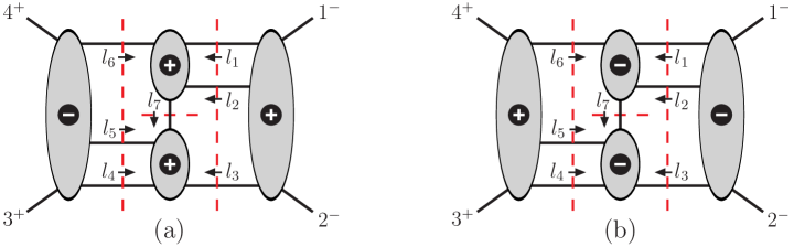
Figure 21: An example of a four-loop planar cut. Case (a) gives the singlet helicity configuration, where only a single gluonic helicity configuration contributes. Case (b) gives non-singlet helicity configurations where all particles in the ${{\cal N}=4}$ multiplet contribute.

To give an illustration of the above rules, we consider supersums in the evaluation of some non-trivial cuts of four-loop amplitudes. First consider the planar generalized cut of the four-loop amplitude $A_{4}^{{\rm 4\hbox{-}loop}}(1^{-},2^{-},3^{+},4^{+})$ shown in fig. 21. There are two distinct configurations of MHV and $\overline{\hbox{MHV}}$ tree amplitudes. Fig. 21(a) is a singlet helicity configuration. The helicity configuration of the internal lines is uniquely fixed once the external lines are specified. Thus, according to our rules only a single term appears in the sum raised to the fourth power. The value of contribution (a) is then,

$$C^{\rm fig.\;\ref{FourLoopPlanarExampleFigure}\rm(a)} = A_{5}^{\rm MHV}(1^{-},2^{-},l_{3}^{+},l_{2}^{+},l_{1}^{+})\,A_{4}^{\rm MHV}(-l_{3}^{-},-l_{4}^{+},-l_{5}^{+},-l_{7}^{-})\,A_{4}^{\rm MHV}(-l_{1}^{-},-l_{2}^{-},l_{7}^{+},-l_{6}^{+})\,$$ (102)

$$\hskip 56.9055pt\times A_{5}^{\rm\overline{MHV}}(3^{+},4^{+},l_{6}^{-},l_{5}^{-},l_{4}^{-})$$

$$= -{\left\langle 1\,2\right\rangle^{4}\over\left\langle 1\,2\right\rangle\left\langle 2\,l_{3}\right\rangle\left\langle l_{3}\,l_{2}\right\rangle\left\langle l_{2}\,l_{1}\right\rangle\left\langle l_{1}\,1\right\rangle}\,{\left\langle l_{3}\,l_{7}\right\rangle^{4}\over\left\langle l_{3}\,l_{4}\right\rangle\left\langle l_{4}\,l_{5}\right\rangle\left\langle l_{5}\,l_{7}\right\rangle\left\langle l_{7}\,l_{3}\right\rangle}$$

$$\hskip 28.45274pt\hbox{}\times{\left\langle l_{2}\,l_{1}\right\rangle^{4}\over\left\langle l_{1}\,l_{2}\right\rangle\left\langle l_{2}\,l_{7}\right\rangle\left\langle l_{7}\,l_{6}\right\rangle\left\langle l_{6}\,l_{1}\right\rangle}\,{\left[3\,4\right]^{4}\over\left[3\,4\right]\left[4\,l_{6}\right]\left[l_{6}\,l_{5}\right]\left[l_{5}\,l_{4}\right]\left[l_{4}\,3\right]}\,.$$

This result is valid for all the gauge multiplet of ${\cal N}\leq 4$ supersymmetric theories, since only gluons contribute here.

Now consider the more complicated case in fig. 21(b) involving non-singlet contributions. We have,

$$C^{\rm fig.\;\ref{FourLoopPlanarExampleFigure}\rm(b)} = \sum_{\rm states}A_{5}^{\rm\overline{MHV}}(1^{-},2^{-},l_{3},l_{2},l_{1})\,A_{4}^{\rm\overline{MHV}}(-l_{3},-l_{4},-l_{5},-l_{7})\,A_{4}^{\rm\overline{MHV}}(-l_{1},-l_{2},l_{7},-l_{6})\,\hskip 19.91684pt$$ (103)

$$\hskip 56.9055pt\times A_{5}^{\rm MHV}(3^{+},4^{+},l_{6},l_{5},l_{4})$$

$$= -\rho^{\rm fig.\;\ref{FourLoopPlanarExampleFigure}\rm(b)}{1\over\left[1\,2\right]\left[2\,l_{3}\right]\left[l_{3}\,l_{2}\right]\left[l_{2}\,l_{1}\right]\left[l_{1}\,1\right]}\,{1\over\left[l_{3}\,l_{4}\right]\left[l_{4}\,l_{5}\right]\left[l_{5}\,l_{7}\right]\left[l_{7}\,l_{3}\right]}$$

$$\hskip 28.45274pt\hbox{}\times{1\over\left[l_{1}\,l_{2}\right]\left[l_{2}\,l_{7}\right]\left[l_{7}\,l_{6}\right]\left[l_{6}\,l_{1}\right]}\,{1\over\left\langle 3\,4\right\rangle\left\langle 4\,l_{6}\right\rangle\left\langle l_{6}\,l_{5}\right\rangle\left\langle l_{5}\,l_{4}\right\rangle\left\langle l_{4}\,3\right\rangle}\,,$$

where $\rho^{\rm fig.\;\ref{FourLoopPlanarExampleFigure}\rm(b)}$ accounts for the sum over multiplet. There are a total of eight distinct purely gluonic helicity configurations, obtained by listing out the non-vanishing possibilities which maintain the holomorphicity of fig. 21(b). Using the rules in the previous section, the gluonic numerator factors can be converted to eight primitive contributions,

$$A=\left\langle l_{4}\,l_{5}\right\rangle\left[l_{4}\,l_{5}\right]\left[l_{2}\,l_{7}\right]\left[l_{1}\,l_{3}\right]\,,\hskip 8.53581ptB=\left\langle l_{4}\,l_{5}\right\rangle\left[l_{4}\,l_{5}\right]\left[l_{7}\,l_{1}\right]\left[l_{2}\,l_{3}\right]\,,\hskip 8.53581ptC=\left\langle l_{4}\,l_{6}\right\rangle\left[l_{4}\,l_{7}\right]\left[l_{2}\,l_{6}\right]\left[l_{1}\,l_{3}\right]\,,$$

$$D=\left\langle l_{4}\,l_{6}\right\rangle\left[l_{4}\,l_{7}\right]\left[l_{6}\,l_{1}\right]\left[l_{2}\,l_{3}\right]\,,\hskip 8.53581ptE=\left\langle l_{5}\,l_{6}\right\rangle\left[l_{5}\,l_{7}\right]\left[l_{2}\,l_{6}\right]\left[l_{1}\,l_{3}\right]\,,\hskip 8.53581ptF=\left\langle l_{5}\,l_{6}\right\rangle\left[l_{5}\,l_{7}\right]\left[l_{6}\,l_{1}\right]\left[l_{2}\,l_{3}\right]\,,$$

$$G=\left\langle l_{4}\,l_{6}\right\rangle\left[l_{2}\,l_{1}\right]\left[l_{3}\,l_{4}\right]\left[l_{6}\,l_{7}\right]\,,\hskip 8.53581ptH=\left\langle l_{5}\,l_{6}\right\rangle\left[l_{2}\,l_{1}\right]\left[l_{3}\,l_{5}\right]\left[l_{6}\,l_{7}\right]\,.$$ (104)

The sum over these eight terms exhibits the supersymmetric cancellations after using Schouten’s identity and momentum conservation,

$$A+B+C+D+E+F+G+H=s\left[l_{1}\,l_{2}\right]\left[l_{7}\,l_{3}\right]\,,$$ (105)

where $s=(k_{1}+k_{2})^{2}$. We may then assemble the supersum for ${\cal N}<4$ following the discussion in section VI.1; using eq. (98) we obtain,

$$\rho^{\rm fig.\;\ref{FourLoopPlanarExampleFigure}\rm(b)}=(s\left[l_{1}\,l_{2}\right]\left[l_{7}\,l_{3}\right])^{\cal N}(A^{4-{\cal N}}+B^{4-{\cal N}}+C^{4-{\cal N}}+D^{4-{\cal N}}+E^{4-{\cal N}}+F^{4-{\cal N}}+G^{4-{\cal N}}+H^{4-{\cal N}}),$$ (106)

which is valid for the minimal ${\cal N}=0,1,2,3$ supersymmetric gauge multiplets. The case ${\cal N}=3$ is equivalent to ${\cal N}=4$,

$$\rho^{\rm fig.\;\ref{FourLoopPlanarExampleFigure}\rm(b)}_{{\cal N}=4}=s^{4}\left[l_{1}\,l_{2}\right]^{4}\left[l_{7}\,l_{3}\right]^{4}\,.$$ (107)

As for the ${\cal N}=4$ three-loop example in section V.5, the ${\cal N}=4$ case (but not ${\cal N}\leq 2$) exhibits the property that the two contributions in fig. 21, are complex conjugates after dividing by an overall factor of the tree amplitude,

$$\frac{iC^{\rm fig.\;\ref{FourLoopPlanarExampleFigure}\rm(b)}_{{\cal N}=4}}{A^{\rm tree}_{4}}=\Biggl{(}\frac{iC^{\rm fig.\;\ref{FourLoopPlanarExampleFigure}\rm(a)}}{A^{\rm tree}_{4}}\Biggr{)}^{*}\,,$$ (108)

where the $i$ is inserted to correct for an overall phase that depends on the loop order.

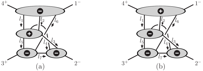
Figure 22: A nontrivial nonplanar cut at four loops. The cuts (a) and (b) represent the two distinct contributions to the cuts. As discussed in the text it using the rules developed here it is straightforward to write down the expression corresponding to these diagrams. All visible legs are on-shell.

As a nonplanar example, consider the cut depicted in fig. 22. As far as the supersums are concerned the planarity or nonplanarity of the cut, is of little consequence, with the only difference appearing in the spinor denominators which are identical for all terms in the sum. This is an especially useful cut because it checks a large number of contributions to the four-loop amplitude, including the most complicated nonplanar integrals. As for previous examples, it turns out that there are two distinct choices of holomorphicity, corresponding to (a) and (b) in fig. 22, since any helicity configuration falls into one of these two classes. In the first class (a) we have seven distinct gluonic helicity choices. In the second class (b) we have eight distinct gluonic helicity choices.

We write down the target expression from the cuts using the above rules. For (a) we have the cut contribution

$$C^{\rm fig.\;\ref{FourLoopNonPlanarExampleFigure}\rm(a)} = \sum_{\rm states}A_{5}^{\rm\overline{MHV}}(1^{-},l_{6},l_{2},l_{1},4^{+})\,A_{5}^{\rm MHV}(-l_{1},l_{4},-l_{2},l_{3},l_{5})\,$$ (109)

$$\hbox{}\times A_{4}^{\rm\overline{MHV}}(-l_{4},-l_{3},2^{-},-l_{7})\,A_{4}^{\rm\overline{MHV}}(-l_{5},-l_{6},l_{7},3^{+})\,,$$

where the ${\cal N}=4$ supersum factor is

$$\rho^{\rm fig.\;\ref{FourLoopNonPlanarExampleFigure}\rm(a)}_{{\cal N}=4} = \biggl{[}\left\langle l_{1}\,l_{4}\right\rangle\left[l_{1}\,4\right]\left[l_{4}\,l_{7}\right]\left[3\,l_{6}\right]+\left\langle l_{1}\,l_{3}\right\rangle\left[l_{1}\,4\right]\left[l_{3}\,l_{7}\right]\left[3\,l_{6}\right]+\left\langle l_{2}\,l_{3}\right\rangle\left[l_{2}\,4\right]\left[l_{3}\,l_{7}\right]\left[3\,l_{6}\right]$$ (110)

$$\hbox{}+\left\langle l_{2}\,l_{4}\right\rangle\left[l_{2}\,4\right]\left[l_{4}\,l_{7}\right]\left[3\,l_{6}\right]+\left\langle l_{3}\,l_{5}\right\rangle\left[l_{3}\,l_{7}\right]\left[l_{5}\,3\right]\left[4\,l_{6}\right]$$

$$\hbox{}+\left\langle l_{4}\,l_{5}\right\rangle\left[l_{4}\,l_{7}\right]\left[l_{5}\,3\right]\left[4\,l_{6}\right]+\left\langle l_{4}\,l_{3}\right\rangle\left[l_{3}\,l_{4}\right]\left[4\,l_{6}\right]\left[3\,l_{7}\right]\biggr{]}^{4}\,.$$

By making repeated use of Schouten’s identity this simplifies to

$$\rho^{\rm fig.\;\ref{FourLoopNonPlanarExampleFigure}\rm(a)}_{{\cal N}=4}=\big{(}\left\langle 1\,2\right\rangle\left[l_{7}\,2\right]\left[l_{6}\,3\right]\left[1\,4\right]\big{)}^{4}\,.$$ (111)

For configuration (b) in fig. 22 we have the contribution,

$$C^{\rm fig.\;\ref{FourLoopNonPlanarExampleFigure}\rm(b)} = \sum_{\rm states}A_{5}^{\rm MHV}(1^{-},l_{6},l_{2},l_{1},4^{+})\,A_{5}^{\rm\overline{MHV}}(-l_{1},l_{4},-l_{2},l_{3},l_{5})\,$$ (112)

$$\hbox{}\times A_{4}^{\rm\overline{MHV}}(-l_{4},-l_{3},2^{-},-l_{7})\,A_{4}^{\rm\overline{MHV}}(-l_{5},-l_{6},l_{7},3^{+})\,.$$

In this case the ${\cal N}=4$ factor from summing over the states crossing the cuts is

$$\rho^{\rm fig.\;\ref{FourLoopNonPlanarExampleFigure}\rm(b)}_{{\cal N}=4} = \biggl{[}\left\langle 1\,l_{6}\right\rangle\left[l_{5}\,l_{3}\right]\left[l_{4}\,l_{7}\right]\left[3\,l_{6}\right]+\left\langle 1\,l_{1}\right\rangle\left[l_{1}\,l_{4}\right]\left[l_{3}\,l_{7}\right]\left[l_{5}\,3\right]$$

$$\hbox{}+\left\langle 1\,l_{2}\right\rangle\left[l_{3}\,l_{7}\right]\left[l_{4}\,l_{2}\right]\left[3\,l_{5}\right]+\left\langle 1\,l_{1}\right\rangle\left[l_{1}\,l_{3}\right]\left[l_{4}\,l_{7}\right]\left[3\,l_{5}\right]+\left\langle 1\,l_{2}\right\rangle\left[l_{2}\,l_{3}\right]\left[l_{4}\,l_{7}\right]\left[3\,l_{5}\right]$$

$$\hbox{}+\left\langle 1\,l_{6}\right\rangle\left[l_{3}\,l_{7}\right]\left[l_{4}\,l_{5}\right]\left[3\,l_{6}\right]+\left\langle 1\,l_{1}\right\rangle\left[l_{1}\,l_{5}\right]\left[l_{3}\,l_{4}\right]\left[3\,l_{7}\right]+\left\langle 1\,l_{2}\right\rangle\left[l_{2}\,l_{5}\right]\left[l_{3}\,l_{4}\right]\left[3\,l_{7}\right]\biggr{]}^{4}\,.$$

After repeatedly applying Schouten’s identity we obtain,

$$\rho^{\rm fig.\;\ref{FourLoopNonPlanarExampleFigure}\rm(b)}_{{\cal N}=4}=\big{(}\left\langle 1\,2\right\rangle\left[2\,3\right]\left[l_{3}\,l_{4}\right]\left[l_{5}\,l_{7}\right]\big{)}^{4}\,.$$ (114)

Although not manifest in the form we present here, the two contributions to the cut in eqs. (109) and (112), satisfy a complex conjugation relation similar to the one in eq. (108). To obtain the nonplanar cuts for the ${\cal N}<4$ supersymmetric theories, we match to the numerator forms in eqs. (110) and (VI.3) to eq. (92) and use the form in eq. (98) to replace the numerators with the appropriate ones.

VII From ${{\cal N}=4}$ super-Yang-Mills theory to ${{\cal N}=8}$ supergravity

Many of the tools presented in previous sections, which were derived from the on-shell superspace of ${{\cal N}=4}$ super-Yang-Mills, carry directly over to ${{\cal N}=8}$ supergravity. For cuts that factorize loop amplitudes into only MHV and $\overline{\hbox{MHV}}$ tree amplitudes, the methods of the previous sections can be generalized to ${{\cal N}=8}$ supergravity by replacing $\delta^{(8)}(Q^{a})\rightarrow\delta^{(16)}(Q^{a})$, and by suitably replacing the other factors in the amplitudes with the crossing symmetric gravity expressions. In this case the $R$-symmetry index runs up to eight. However, at present the existence of a complete set of MHV expansion rules for gravity has not been fully established FreedmanGenerating . As such, there are many gravity cuts that cannot be handled directly by relying on an MHV expansion. One may use the BCFW recursion form of the tree-level superamplitudes in the unitarity cuts, but this has not been studied systematically beyond one loop AHCKGravity ; N8TreeSuperAmplitude . Furthermore, the issue of four-dimensional cuts being insufficient for reconstructing the $D$-dimensional amplitude is more pressing in the case of gravity. The presence of twice as many powers of momenta in the numerators of gravity diagrams, compared to gauge theory, offers more possibilities for expressions that vanish in four dimensions, but not in $D$ dimensions, to appear in the cuts. An example of such an object is the Gram determinant $\det(p_{i}\cdot p_{j})$, with at least five independent momenta (including loop momenta).

A method that effectively tackles both of these problem is described in refs. BDDPR ; GravityThree : the tree level Kawai-Lewellen-Tye (KLT ) relations can be used to relate cuts of ${{\cal N}=8}$ supergravity to sums of products of cuts ${{\cal N}=4}$ super-Yang-Mills theory, with additional kinematic factors. Since the KLT relations are valid in $D$ dimensions, the gravity cuts determined through their use will automatically be valid in arbitrary dimensions if the corresponding Yang-Mills cuts are.

Schematically, the KLT relations are of the form

$$M_{n}^{\rm tree}=\sum_{i,j}g_{ij}A_{n}^{(i)}A_{n}^{(j)}\,,$$ (115)

where $M^{\rm tree}_{n}$ is an $n$-point ${{\cal N}=8}$ supergravity amplitude, the $A_{n}^{(i)}$ are color-stripped $n$-point tree amplitudes in ${{\cal N}=4}$ super-Yang-Mills theory labeled by an index $i$, implicitly incorporating all labels appearing in the amplitudes. The $g_{ij}$ are polynomials in kinematic invariants $s_{lm}=(k_{l}+k_{m})^{2}$ of degree $(n-3)$. The precise form of the relations for any number of external legs may be found in ref. OneloopMHVGravity . While their derivation from the (super)gravity Lagrangian remains obscure, it was recently shown that the KLT relations are equivalent to relations between numerator factors of individual tree diagrams TreeJacobi .

Generalized unitarity cuts in ${{\cal N}=8}$ supergravity are constructed, in much the same way as in ${{\cal N}=4}$ SYM, as products of tree-level amplitudes. Because the ${{\cal N}=8}$ supergravity multiplet is the tensor product of two ${{\cal N}=4}$ super-Yang-Mills vector multiplets, when applying the KLT relations, the supersymmetric sums appearing in the cuts for supergravity amplitudes can be re-expressed as two copies of supersymmetric sums for Yang-Mills amplitudes. For example, for a cut that breaks the amplitude into two tree amplitudes we have BDDPR ,

$$M_{n}^{L\rm-loop}\Bigr{|}_{\rm cut}=\sum_{{{\cal N}=8}}M_{n_{1}}^{\rm tree}M_{n_{2}}^{\rm tree} = \sum_{{{\cal N}=8}}\left(\sum_{i,j}g_{ij}A_{n_{1}}^{(i)}A_{n_{1}}^{(j)}\right)\left(\sum_{k,l}g_{kl}A_{n_{2}}^{(k)}A_{n_{2}}^{(l)}\right)$$ (116)

$$= \sum_{i,j,k,l}g_{ij}g_{kl}\left(\sum_{{{\cal N}=4}}A_{n_{1}}^{(i)}A_{n_{2}}^{(k)}\right)\left(\sum_{{{\cal N}=4}}A_{n_{1}}^{(j)}A_{n_{2}}^{(l)}\right)\,,$$ (117)

where the $\sum_{{{\cal N}=4}}A_{n_{1}}^{(i)}A_{n_{2}}^{(k)}$ are color-stripped cuts of ${{\cal N}=4}$ super-Yang-Mills amplitudes. Any cut which decomposes a loop amplitude into a product of trees works similarly. Thus, instead of evaluating the supergravity cuts starting from $D$-dimensional supergravity tree amplitudes, it is generally more efficient to assemble them from simpler cuts of the Yang-Mills amplitude via the KLT relations  CompactThree .

Since the KLT relations also hold for gravity theories with fewer supersymmetries than the maximal number, the gauge theory discussion in section VI.1 can be carried over to gravity as well. Whenever a gravity theory is the low-energy limit of a string theory, we are guaranteed that the KLT relations will hold; this includes the vast number of heterotic string constructions Heterotic . The relations appear to apply even more generally than dictated by the heterotic string constructions GeneralKLT . In general, the KLT construction may give undesirable states in the tensor product, such as an dilaton and antisymmetric tensor in the ${\cal N}=0$ case; to remove their contributions additional projections would be required.

VIII Conclusions

In this paper we described techniques for evaluating sums over the multiplet of states appearing in the four-dimensional generalized unitarity cuts of multi-loop super-Yang-Mills amplitudes. We used these techniques to expose general features of the cut amplitudes.

Our approach for evaluating the supersums in cuts is inspired by the one of Bianchi, Elvang, Kiermaier and Freedman FreedmanGenerating ; FreedmanUnitarity and based on the MHV expansion of tree amplitudes CSW ; GGK ; FreedmanProof . Here we reorganized the contributions in two ways: first, as a linear system of algebraic equations, and, in the second, in terms of diagrams tracking the flow of $SU(4)$ $R$-symmetry indices. An important advantage of the algebraic approach is that simplifications based on Schouten’s identity are obtained automatically. This is a natural approach for carrying out formal derivations of properties of amplitudes. On the other hand, the diagrammatic approach makes it straightforward to construct results by drawing simple diagrams and leads to an easily programmable algorithm for evaluating supersums by sweeping over possible purely gluonic configurations. The expressions obtained this way can be further simplified through use of Schouten’s identity and momentum conservation; we described graphical rules for carrying out such manipulations, whose effect is to improve the power count by replacing some of the numerator loop momenta of cuts with external momenta.

We also used the index-diagram approach to construct a generating function for certain theories with less-than-maximal supersymmetry. This is straightforward because the index-diagram approach tracks the contributions of individual configurations of states in the cuts. This allowed us to give simple rules determining the contributions of various gauge multiplets to cuts. It should be possible to further generalize these considerations to supersymmetric theories with arbitrary matter content.

In general, completely determining the integrand of amplitudes requires the evaluation of unitarity cuts in an arbitrary number of dimensions. In particular, use of dimensional regularization to control infrared or ultraviolet singularities implies that the amplitudes cannot be evaluated in strictly four dimensions. Nevertheless, in practical calculations, four-dimensional cuts provide invaluable guidance for constructing an ansatz, whose cuts can be verified through the more complicated $D$ dimensional cuts. The efficient and systematic evaluation of supermultiplet sums in arbitrary dimensions remains an important open problem. One obstacle arises from the strong dependence of on-shell superspaces on the specific dimensionality of space-time, making it difficult to treat all dimensions in a unified way. Another difficulty is the absence of a formalism as efficient as four-dimensional spinor helicity in general dimensions. Recent progress towards solving the latter problem is given in ref. D6Helicity , where a six-dimensional helicity-like formalism is constructed.

The KLT KLT ; GeneralKLT ; TreeJacobi relations allow us to rewrite any product of tree-level amplitudes in ${{\cal N}=8}$ supergravity representing the generalized cut of some multi-loop amplitude directly in terms of double products of cuts of ${{\cal N}=4}$ super-Yang-Mills amplitudes BDDPR . This allows us to immediately carry over to ${{\cal N}=8}$ supergravity ${{\cal N}=4}$ super-Yang-Mills evaluations of supersums. Higher-loop studies of ${{\cal N}=8}$ supergravity should help shed further light on the recent proposal that ${{\cal N}=8}$ supergravity may be a perturbatively finite theory of quantum gravity Finite ; DualityArguments ; GravityThree .

In summary, the techniques presented here clarify the structure of unitarity cuts in supersymmetric theories. These should be helpful in future studies of the properties of multi-loop amplitudes via the unitarity method. In particular these methods are important parts of the construction of the four-loop four-point nonplanar amplitudes of ${{\cal N}=4}$ super-Yang-Mills theory FourLoopNonPlanar , which will probe the multiloop infrared and ultraviolet structures of gauge theories, and aid in the construction of the corresponding ${{\cal N}=8}$ supergravity amplitudes. These amplitudes will allow for a definitive determination of the four-loop ultraviolet behavior of the two maximally supersymmetric theories in various dimensions.

References

- (1) Z. Bern, M. Czakon, L. J. Dixon, D. A. Kosower and V. A. Smirnov, Phys. Rev. D 75, 085010 (2007) [hep-th/0610248].
- (2) C. Anastasiou, Z. Bern, L. J. Dixon and D. A. Kosower, Phys. Rev. Lett. 91, 251602 (2003) [hep-th/0309040].
- (3) Z. Bern, L. J. Dixon and V. A. Smirnov, Phys. Rev. D 72, 085001 (2005) [hep-th/0505205].
- (4) L. F. Alday and J. Maldacena, JHEP 0706, 064 (2007) [0705.0303 [hep-th]];
-
(5)
J. M. Maldacena,
Adv. Theor. Math. Phys. 2, 231 (1998)
[Int. J. Theor. Phys. 38, 1113 (1999)]
[hep-th/9711200];
S. S. Gubser, I. R. Klebanov and A. M. Polyakov, Phys. Lett. B 428, 105 (1998) [hep-th/9802109];
O. Aharony, S. S. Gubser, J. M. Maldacena, H. Ooguri and Y. Oz, Phys. Rept. 323, 183 (2000) [hep-th/9905111]. - (6) Z. Bern, L. J. Dixon and R. Roiban, Phys. Lett. B 644, 265 (2007) [hep-th/0611086].
- (7) Z. Bern, J. J. Carrasco, L. J. Dixon, H. Johansson, D. A. Kosower and R. Roiban, Phys. Rev. Lett. 98, 161303 (2007) [hep-th/0702112].
- (8) Z. Bern, J. J. M. Carrasco, L. J. Dixon, H. Johansson and R. Roiban, 0808.4112 [hep-th].
-
(9)
F. Cachazo, M. Spradlin and A. Volovich,
Phys. Rev. D 74, 045020 (2006)
[hep-th/0602228];
Z. Bern, M. Czakon, D. A. Kosower, R. Roiban and V. A. Smirnov, Phys. Rev. Lett. 97, 181601 (2006) [hep-th/0604074]. - (10) J. M. Drummond, J. Henn, G. P. Korchemsky and E. Sokatchev, 0712.1223 [hep-th].
-
(11)
J. M. Drummond, J. Henn, V. A. Smirnov and E. Sokatchev,
JHEP 0701, 064 (2007)
[hep-th/0607160];
J. M. Drummond, G. P. Korchemsky and E. Sokatchev, Nucl. Phys. B 795, 385 (2008) [0707.0243 [hep-th]];
A. Brandhuber, P. Heslop and G. Travaglini, Nucl. Phys. B 794, 231 (2008) [0707.1153 [hep-th]];
J. M. Drummond, J. Henn, G. P. Korchemsky and E. Sokatchev, Nucl. Phys. B 795, 52 (2008) [0709.2368 [hep-th]]. - (12) Z. Bern, J. J. M. Carrasco, H. Johansson and D. A. Kosower, Phys. Rev. D 76, 125020 (2007) [0705.1864 [hep-th]].
- (13) J. M. Drummond, J. M. Henn and J. Plefka, 0902.2987 [hep-th].
-
(14)
N. Berkovits and J. Maldacena,
JHEP 0809, 062 (2008)
[0807.3196 [hep-th]];
N. Beisert, R. Ricci, A. A. Tseytlin and M. Wolf, Phys. Rev. D 78, 126004 (2008) [0807.3228 [hep-th]];
N. Beisert, 0903.0609 [hep-th]. - (15) L. F. Alday and J. Maldacena, JHEP 0711, 068 (2007) [0710.1060 [hep-th]].
-
(16)
J. Bartels, L. N. Lipatov and A. Sabio Vera,
0802.2065 [hep-th];
R. C. Brower, H. Nastase, H. J. Schnitzer and C. I. Tan, 0809.1632 [hep-th];
V. Del Duca, C. Duhr and E. W. N. Glover, JHEP 0812, 097 (2008) [0809.1822 [hep-th]]. - (17) Z. Bern, L. J. Dixon, D. A. Kosower, R. Roiban, M. Spradlin, C. Vergu and A. Volovich, Phys. Rev. D 78, 045007 (2008) [0803.1465 [hep-th]].
-
(18)
S. Mert Aybat, L. J. Dixon and G. Sterman,
Phys. Rev. Lett. 97, 072001 (2006)
[hep-ph/0606254];
Phys. Rev. D 74, 074004 (2006)
[hep-ph/0607309];
T. Becher and M. Neubert, 0901.0722 [hep-ph]; 0903.1126 [hep-ph];
E. Gardi and L. Magnea, 0901.1091 [hep-ph];
L. J. Dixon, 0901.3414 [hep-ph]. -
(19)
E. Cremmer, B. Julia and J. Scherk,
Phys. Lett. B 76, 409 (1978);
E. Cremmer and B. Julia, Phys. Lett. B 80, 48 (1978); Nucl. Phys. B 159, 141 (1979). - (20) Z. Bern, L. J. Dixon and D. A. Kosower, Nucl. Phys. B 513, 3 (1998) [hep-ph/9708239]; Z. Bern, V. Del Duca, L. J. Dixon and D. A. Kosower, Phys. Rev. D 71, 045006 (2005) [hep-th/0410224].
- (21) Z. Bern, L. J. Dixon and D. A. Kosower, JHEP 0408, 012 (2004) [hep-ph/0404293].
-
(22)
R. Britto, F. Cachazo and B. Feng,
Nucl. Phys. B 725, 275 (2005)
[hep-th/0412103];
E. I. Buchbinder and F. Cachazo, JHEP 0511, 036 (2005) [hep-th/0506126]. - (23) Z. Bern, L. J. Dixon, M. Perelstein and J. S. Rozowsky, Nucl. Phys. B 546, 423 (1999) [hep-th/9811140].
-
(24)
Z. Bern, N. E. J. Bjerrum-Bohr and D. C. Dunbar,
JHEP 0505, 056 (2005)
[hep-th/0501137];
N. E. J. Bjerrum-Bohr, D. C. Dunbar and H. Ita, Phys. Lett. B 621, 183 (2005) [hep-th/0503102];
N. E. J. Bjerrum-Bohr, D. C. Dunbar, H. Ita, W. B. Perkins and K. Risager, JHEP 0612, 072 (2006) [hep-th/0610043];
R. Kallosh, 0711.2108 [hep-th];
N. E. J. Bjerrum-Bohr and P. Vanhove, JHEP 0804, 065 (2008) [0802.0868 [hep-th]]; N. E. J. Bjerrum-Bohr and P. Vanhove, 0805.3682 [hep-th]; 0806.1726 [hep-th]. - (25) Z. Bern, J. J. Carrasco, D. Forde, H. Ita and H. Johansson, Phys. Rev. D 77, 025010 (2008) [0707.1035 [hep-th]].
- (26) N. Arkani-Hamed, F. Cachazo and J. Kaplan, 0808.1446 [hep-th].
-
(27)
G. Chalmers,
hep-th/0008162;
M. B. Green, J. G. Russo and P. Vanhove, JHEP 0702, 099 (2007) [hep-th/0610299]. - (28) N. Berkovits, Phys. Rev. Lett. 98, 211601 (2007) [hep-th/0609006].
- (29) M. B. Green, J. G. Russo and P. Vanhove, Phys. Rev. Lett. 98, 131602 (2007) [hep-th/0611273].
- (30) M. B. Green, H. Ooguri and J. H. Schwarz, Phys. Rev. Lett. 99, 041601 (2007) [0704.0777 [hep-th]].
- (31) G. Bossard, P. S. Howe and K. S. Stelle, 0901.4661 [hep-th].
- (32) Z. Bern, L. J. Dixon, D. C. Dunbar and D. A. Kosower, Nucl. Phys. B 425, 217 (1994) [hep-ph/9403226].
- (33) Z. Bern, L. J. Dixon, D. C. Dunbar and D. A. Kosower, Nucl. Phys. B 435, 59 (1995) [hep-ph/9409265].
-
(34)
F. Cachazo and D. Skinner,
0801.4574 [hep-th];
F. Cachazo, 0803.1988 [hep-th]. - (35) M. Bianchi, H. Elvang and D. Z. Freedman, 0805.0757 [hep-th].
- (36) H. Elvang, D. Z. Freedman and M. Kiermaier, 0808.1720 [hep-th].
- (37) J. M. Drummond, J. Henn, G. P. Korchemsky and E. Sokatchev, 0808.0491 [hep-th].
- (38) Z. Bern, J. J. Carrasco, L. J. Dixon, H. Johansson, and R. Roiban, to appear.
- (39) Z. Bern, J. S. Rozowsky and B. Yan, Phys. Lett. B 401, 273 (1997) [hep-ph/9702424].
- (40) Z. Bern, L. J. Dixon, D. C. Dunbar, M. Perelstein and J. S. Rozowsky, Nucl. Phys. B 530, 401 (1998) [hep-th/9802162].
-
(41)
M. T. Grisaru, H. N. Pendleton and P. van Nieuwenhuizen,
Phys. Rev. D 15, 996 (1977);
M. T. Grisaru and H. N. Pendleton, Nucl. Phys. B 124, 81 (1977);
S. J. Parke and T. R. Taylor, Phys. Lett. B 157, 81 (1985) [Erratum-ibid. 174B, 465 (1986)]. -
(42)
F. Cachazo, M. Spradlin and A. Volovich,
0805.4832 [hep-th];
M. Spradlin, A. Volovich and C. Wen, 0808.1054 [hep-th]. - (43) V. P. Nair, Phys. Lett. B 214, 215 (1988).
-
(44)
G. Georgiou, E. W. N. Glover and V. V. Khoze,
JHEP 0407, 048 (2004)
[hep-th/0407027];
Y. t. Huang, Phys. Lett. B 631, 177 (2005) [hep-th/0507117];
H. Feng and Y. t. Huang, hep-th/0611164. - (45) M. Kiermaier, H. Elvang and D. Z. Freedman, 0811.3624 [hep-th].
- (46) F. Cachazo, P. Svrcek and E. Witten, JHEP 0409, 006 (2004) [hep-th/0403047].
-
(47)
J. M. Drummond, J. Henn, G. P. Korchemsky and E. Sokatchev,
0807.1095 [hep-th];
A. Brandhuber, P. Heslop and G. Travaglini, 0807.4097 [hep-th];
J. M. Drummond and J. M. Henn, 0808.2475 [hep-th]. -
(48)
R. Britto, F. Cachazo and B. Feng,
Nucl. Phys. B 715, 499 (2005)
[hep-th/0412308];
R. Britto, F. Cachazo, B. Feng and E. Witten, Phys. Rev. Lett. 94, 181602 (2005) [hep-th/0501052]. - (49) M. Kiermaier and S. G. Naculich, 0903.0377 [hep-th].
-
(50)
S. Mandelstam,
Nucl. Phys. B 213, 149 (1983);
P. S. Howe and K. S. Stelle, Int. J. Mod. Phys. A 4, 1871 (1989);
N. Marcus and A. Sagnotti, Nucl. Phys. B 256, 77 (1985). -
(51)
Z. Bern and A. G. Morgan,
Nucl. Phys. B 467, 479 (1996)
[hep-ph/9511336];
Z. Bern, L. J. Dixon and D. A. Kosower, Ann. Rev. Nucl. Part. Sci. 46, 109 (1996) [hep-ph/9602280];
Z. Bern, L. J. Dixon and D. A. Kosower, JHEP 0001, 027 (2000) [hep-ph/0001001]. - (52) Z. Bern, L. J. Dixon, D. C. Dunbar and D. A. Kosower, Phys. Lett. B 394, 105 (1997) [hep-th/9611127].
-
(53)
Z. Bern and D. A. Kosower,
Nucl. Phys. B 379, 451 (1992);
Z. Bern, A. De Freitas, L. J. Dixon and H. L. Wong, Phys. Rev. D 66, 085002 (2002) [hep-ph/0202271]. - (54) W. Siegel, Phys. Lett. B84:193 (1979).
-
(55)
F. A. Berends, R. Kleiss, P. De Causmaecker, R. Gastmans and T. T. Wu,
Phys. Lett. B 103, 124 (1981);
P. De Causmaecker, R. Gastmans, W. Troost and T. T. Wu, Nucl. Phys. B 206, 53 (1982);
Z. Xu, D. H. Zhang and L. Chang, TUTP-84/3-TSINGHUA;
R. Kleiss and W. J. Stirling, Nucl. Phys. B 262, 235 (1985);
J. F. Gunion and Z. Kunszt, Phys. Lett. B 161, 333 (1985);
Z. Xu, D. H. Zhang and L. Chang, Nucl. Phys. B 291, 392 (1987). -
(56)
H. Kawai, D. C. Lewellen and S. H. H. Tye,
Nucl. Phys. B 269, 1 (1986);
Z. Bern and A. K. Grant, Phys. Lett. B 457, 23 (1999) [hep-th/9904026];
Z. Bern, Living Rev. Rel. 5, 5 (2002) [gr-qc/0206071];
N. E. J. Bjerrum-Bohr, Phys. Lett. B 560, 98 (2003) [hep-th/0302131]; Nucl. Phys. B 673, 41 (2003) [hep-th/0305062];
N. E. J. Bjerrum-Bohr and K. Risager, Phys. Rev. D 70, 086011 (2004) [hep-th/0407085];
S. Ananth and S. Theisen, Phys. Lett. B 652, 128 (2007) [0706.1778 [hep-th]];
H. Elvang and D. Z. Freedman, JHEP 0805, 096 (2008) [0710.1270 [hep-th]];
M. Spradlin, A. Volovich and C. Wen, 0812.4767 [hep-th]. - (57) Z. Bern, A. De Freitas and H. L. Wong, Phys. Rev. Lett. 84, 3531 (2000) [hep-th/9912033].
- (58) Z. Bern, J. J. M. Carrasco and H. Johansson, 0805.3993 [hep-ph].
- (59) N. E. J. Bjerrum-Bohr, D. C. Dunbar, H. Ita, W. B. Perkins and K. Risager, JHEP 0601, 009 (2006) [hep-th/0509016].
-
(60)
J. Bedford, A. Brandhuber, B. J. Spence and G. Travaglini,
Nucl. Phys. B 721, 98 (2005)
[hep-th/0502146];
F. Cachazo and P. Svrcek, hep-th/0502160;
P. Benincasa, C. Boucher-Veronneau and F. Cachazo, JHEP 0711, 057 (2007) [hep-th/0702032];
P. Benincasa and F. Cachazo, 0705.4305 [hep-th];
A. Hall, Phys. Rev. D 77, 124004 (2008) [0803.0215 [hep-th]]. -
(61)
Z. Bern, D. Forde, D. A. Kosower and P. Mastrolia,
Phys. Rev. D 72, 025006 (2005)
[hep-ph/0412167];
Z. Bern, L. J. Dixon and D. A. Kosower, Phys. Rev. D 72, 125003 (2005) [hep-ph/0505055]. - (62) E. Witten, Commun. Math. Phys. 252, 189 (2004) [hep-th/0312171].
- (63) K. Risager, JHEP 0512, 003 (2005) [hep-th/0508206].
-
(64)
A. Gorsky and A. Rosly,
JHEP 0601, 101 (2006)
[hep-th/0510111];
P. Mansfield, JHEP 0603, 037 (2006) [hep-th/0511264]. - (65) J. H. Ettle, T. R. Morris and Z. Xiao, JHEP 0808, 103 (2008) [0805.0239 [hep-th]].
-
(66)
R. Boels, L. Mason and D. Skinner,
JHEP 0702, 014 (2007)
[hep-th/0604040];
H. Feng and Y. t. Huang, hep-th/0611164. - (67) D. A. Kosower, Phys. Rev. D 71, 045007 (2005) [hep-th/0406175].
- (68) I. Bena, Z. Bern and D. A. Kosower, Phys. Rev. D 71, 045008 (2005) [hep-th/0406133].
- (69) C. Cheung and D. O’Connell, 0902.0981 [hep-th].
- (70) R. Roiban, M. Spradlin and A. Volovich, Phys. Rev. D 70, 026009 (2004) [hep-th/0403190].
- (71) P. S. Howe and K. S. Stelle, Phys. Lett. B 554, 190 (2003) [hep-th/0211279].
-
(72)
W. Nahm,
Nucl. Phys. B 135, 149 (1978);
E. Witten, Phys. Lett. B 77, 394 (1978);
A. Galperin, E. Ivanov, S. Kalitsyn, V. Ogievetsky and E. Sokatchev, Phys. Lett. B 151, 215 (1985). -
(73)
M. Bershadsky, Z. Kakushadze and C. Vafa,
Nucl. Phys. B 523, 59 (1998)
[hep-th/9803076];
M. Bershadsky and A. Johansen, Nucl. Phys. B 536, 141 (1998) [hep-th/9803249]. - (74) J. M. Drummond, M. Spradlin, A. Volovich and C. Wen, 0901.2363 [hep-th].
-
(75)
D. J. Gross, J. A. Harvey, E. J. Martinec and R. Rohm,
Nucl. Phys. B 256, 253 (1985);
L. J. Dixon, J. A. Harvey, C. Vafa and E. Witten, Nucl. Phys. B 261, 678 (1985);
K. S. Narain, Phys. Lett. B 169, 41 (1986);
H. Kawai, D. C. Lewellen and S. H. H. Tye, Nucl. Phys. B 288, 1 (1987);
I. Antoniadis, C. P. Bachas and C. Kounnas, Nucl. Phys. B 289, 87 (1987).