Repulsive Fermi gas in a harmonic trap: Ferromagnetism and spin textures

Abstract

We study ferromagnetism in a repulsively interacting two-component Fermi gas in a harmonic trap. Within a local density approximation, the two components phase-separate beyond a critical interaction strength, with one species having a higher density at the trap center. We discuss several easily observable experimental signatures of this transition. The mean field release energy, its separate kinetic and interaction contributions, as well as the potential energy, all depend on the interaction strength and contain a sharp signature of this transition. In addition, the conversion rate of atoms to molecules, arising from three-body collisions, peaks at an interaction strength just beyond the ferromagnetic transition point. We then go beyond the local density approximation, and derive an energy functional which includes a term that depends on the local magnetization gradient and acts as a ‘surface tension’. Using this energy functional, we numerically study the energetics of some candidate spin textures which may be stabilized in a harmonic trapping potential at zero net magnetization. We find that a hedgehog state has a lower energy than an ‘in-out’ domain wall state in an isotropic trap. Upon inclusion of trap anisotropy we find that the hedgehog magnetization profile gets distorted due to the surface tension term, this distortion being more apparent for small atom numbers. We estimate that the magnetic dipole interaction does not play a significant role in this system. We consider possible implications for experiments on trapped ⁶Li and ⁴⁰K gases.

I Introduction

In recent years, a series of beautiful experiments have shown that a gas of two-component fermions interacting via a Feshbach resonance exhibits a superfluid state at low temperature greiner03 ; bourdel03 ; gupta03 ; zweirlein05 . An exciting new direction for cold atoms experiments is the study of ferromagnetism arising from repulsive interactions in a two-component Fermi gas. Such a ferromagnetic ‘Stoner instability’ stoner33 occurs, within mean field theory of a homogeneous Fermi gas at zero temperature, when the (repulsive) s-wave scattering length, $a_{S}$, between two spin states is large enough that $k_{F}a_{S}>\pi/2$, where $\hbar k_{F}$ is the Fermi momentum of the gas. This condition can be satisfied upon tuning $a_{S}$ to large positive values near a Feshbach resonance provided the system stays stable for a sufficiently long time. Since ferromagnetism arises from two-body interactions, whereas atom loss due to Feshbach molecule formation is because of three-body collisions dpetrov03 , there may be a range of densities where the lifetime is long enough to reach the ferromagnetic state.

The suggestion that ferromagnetism may be achieved, as a metastable state, in cold Fermi gases is not new. Salasnich and co-workers salasnich00 have studied the mean field theory of a harmonically trapped Fermi gas with repulsive interactions and found that this should lead to phase separation between the two spin species if the net magnetization is zero. A similar study was carried out by Sogo and Yabu sogo02 allowing for non-zero spontaneous magnetization. Duine and MacDonald duine05 later showed that the ferromagnetic transition in a homogeneous Fermi gas changes from a continuous to a first order transition at low enough temperatures upon going beyond mean field theory. They also proposed that an initially magnetized Fermi gas will tend to stay spin-coherent for long times, even in the presence of magnetic field noise that is naïvely expected to cause strong dephasing, provided the system is close to the transition into a ferromagnetic state duine05 .

Using an optical lattice and engineering the band structure to get flat (dispersionless) bands is another interesting route to achieving ferromagnetism. Such ‘flat-band ferromagnetism’ tasaki98 has the advantage that the ferromagnetic state occurs at weak repulsive interactions and can be theoretically analyzed in a reliable fashion; however, an existing theoretical proposal along these lines involves working with fermions in the p-band of a honeycomb optical lattice congjun08 which is a significant experimental challenge. A recent work coleman08 has considered the possibility of ferromagnetism for strongly interacting fermions in optical lattices and studied, within a phenomenological Landau theory, the energetics of possible spin textures (such as hedgehog states, domain walls and skyrmions) which might arise in a trap.

In this paper, motivated by earlier work and by ongoing experimental efforts, we revisit the problem of ferromagnetism in a harmonically trapped two-component Fermi gas. We begin by using a “local density approximation” (LDA), sometimes referred to in the literature as the Thomas-Fermi approximation, to describe this system. Within the LDA, we find that the mean field release energy of the trapped gas (as well as the potential energy and the kinetic energy component of the release energy) provides a simple, albeit indirect, diagnostic of the ferromagnetic transition. We find that the formation of nonzero local magnetization in the trap causes a suppression of the atom loss rate via three-body collisions. This suppression competes with the growth of the loss rate as the interactions get stronger, leading to a peak in the atom loss rate at an interaction strength which is very close to, but slightly beyond, the ferromagnetic transition point. We then show how one might incorporate magnetization gradient (or ‘surface tension’) terms in order to go beyond the LDA. Our energy functional is akin to an earlier phenomenological Landau theory for ferromagnetism in an optical lattice coleman08 but explicitly keeps track of the spatial dependence of all the Landau theory coefficients which arise from density variations in the trap. Using this extended energy functional, we study the energetics of various spin textures in the case where the net magnetization, which does not relax in these quantum gases, is assumed to be zero. This corresponds to choosing the initial population to be the same for both hyperfine species of fermions. We show, in this case, that a hedgehog configuration of the magnetization has a lower energy than an ‘in-out’ phase-separated configuration with a domain wall. A similar phenomenon has been predicted for fermions in optical lattices coleman08 . Finally, we turn to the effect of anisotropic trapping frequencies in a harmonic trap. While such anisotropies can be incorporated by a trivial rescaling of coordinates in the LDA, this is no longer true in the presence of surface tension which leads to a breakdown of the LDA. (A breakdown of the LDA has been observed hulet06 and theoretically addressed emueller ; demler06 ; sensarma07 in the context of polarized superfluids in highly anisotropic traps.) We use our extended energy functional to numerically study how the hedgehog state distorts upon going from a spherically symmetric trap to an anisotropic cigar-shaped trap. We conclude with estimates which indicate that the magnetic dipole interaction between atoms can be neglected for ⁶Li and ⁴⁰K.

II Ferromagnetism within the local density approximation

The Hamiltonian describing a uniform two-component Fermi gas interacting through a repulsive s-wave contact interaction is given by

$$H\!=\!\sum_{\sigma}\!\int\!\frac{d^{3}{{\bf{K}}}}{(2\pi)^{3}}\epsilon_{{\bf{K}}}c^{\dagger}_{{{\bf{K}}}\sigma}c^{{\phantom{\dagger}}}_{{{\bf{K}}}\sigma}\!\!+\!g\int\!\!d^{3}{{\bf{R}}}c^{\dagger}_{{{\bf{R}}}\uparrow}c^{\dagger}_{{{\bf{R}}}\downarrow}c^{\phantom{\dagger}}_{{{\bf{R}}}\downarrow}c^{\phantom{\dagger}}_{{{\bf{R}}}\uparrow},$$ (1)

where $\epsilon_{{\bf{K}}}=\hbar^{2}{{\bf{K}}}^{2}/2M$ is the kinetic energy of atoms with mass $M$ and momentum $\hbar{{\bf{K}}}$. For a Fermi gas with $N_{\sigma}$ particles of spin-$\sigma$, the uniform gas densities of each spin is $\rho_{\sigma}=N_{\sigma}/{\cal V}$, and the total kinetic energy of the uniform gas is just

$$K=\frac{3}{5}{\cal V}(E_{F\uparrow}\rho_{\uparrow}+E_{F\downarrow}\rho_{\downarrow}),$$ (2)

where ${\cal V}$ denotes the system volume, and $E_{F\sigma}=\alpha\rho_{\sigma}^{2/3}$, with $\alpha=(6\pi^{2})^{2/3}\hbar^{2}/2M$, denotes the Fermi energy of particles with spin-$\sigma$. A mean field theory of the interacting Hamiltonian yields the total interaction energy

$$U=g{\cal V}\rho_{\uparrow}\rho_{\downarrow}.$$ (3)

At this level of treatment the contact interaction strength $g$ is related to the two-body scattering length $a_{S}$ in vacuum via $g=4\pi a_{S}\hbar^{2}/M$.

The local density approximation (LDA) for a trapped Fermi gas corresponds to simply assuming that the above results apply locally in the presence of a trap potential $V({{\bf{R}}})$. The ground state energy of this trapped Fermi gas is then obtained by minimizing the energy functional

$$E[\{\rho_{\sigma}({{\bf{R}}})\}]\!\! = \!\!\int\!\!d^{3}{{\bf{R}}}\!\!\left[\frac{3}{5}\alpha\sum_{\sigma}\rho_{\sigma}^{5/3}({{\bf{R}}})\!+\!g\rho_{\uparrow}({{\bf{R}}})\rho_{\downarrow}({{\bf{R}}})\right.$$ (4)

$$+ \!\!\left.V({{\bf{R}}})\sum_{\sigma}\rho_{\sigma}({{\bf{R}}})-\sum_{\sigma}\mu_{\sigma}\rho_{\sigma}({{\bf{R}}})\right],$$

where $\{\rho_{\sigma}({{\bf{R}}})\}$ denotes the density profile of both spin species $[\rho_{\uparrow}({{\bf{R}}}),\rho_{\downarrow}({{\bf{R}}})]$. Here we have introduced two Lagrange multipliers $\mu_{\sigma}$ which act as chemical potentials for the two spin species and serve to impose the constraints $\int d^{3}{{\bf{R}}}\rho_{\sigma}({{\bf{R}}})=N_{\sigma}$. The separate constraint on each spin component arises from the assumption that the two spin components correspond to the lowest two Zeeman split hyperfine levels of a Fermi gas. Since the Zeeman splitting near a Feshbach resonance is typically far greater than all other energy scales and the total energy must be conserved in these thermally isolated gases, we arrive at the constraint that the population of the two Zeeman components cannot change for fermionic atoms where the only interaction is between different spin components. Thus, unlike in solid state ferromagnets, the magnetization can be conserved on very long time scales.

II.1 Rescaling to the isotropic problem for a harmonic trap

Let us assume that the trapping potential is harmonic, but possibly anisotropic, so that $V({{\bf{R}}})=\frac{1}{2}M\sum_{i}\omega_{i}^{2}{{\bf{R}}}_{i}^{2}$. Here $\omega_{x,y,z}$ are the trapping frequencies along different directions. In order to make the problem appear isotropic we can rescale distances by setting ${\tilde{\bf{R}}}_{i}={{\bf{R}}}_{i}(\omega_{i}/\Omega)$, where $\Omega=(\omega_{x}\omega_{y}\omega_{z})^{1/3}$ is the geometric mean of the trap frequencies. With this standard rescaling, we get

$$E[\{\rho_{\sigma}({\tilde{\bf{R}}})\}] \!\!=\!\! \!\!\int\!\!d^{3}{\tilde{\bf{R}}}\!\!\left[\frac{3}{5}\alpha\sum_{\sigma}\rho_{\sigma}^{5/3}({\tilde{\bf{R}}})+g\rho_{\uparrow}({\tilde{\bf{R}}})\rho_{\downarrow}({\tilde{\bf{R}}})\right.$$ (5)

$$+ \left.\!\!\frac{1}{2}M\Omega^{2}{\tilde{\bf{R}}}^{2}\sum_{\sigma}\rho_{\sigma}({\tilde{\bf{R}}})\!-\!\sum_{\sigma}\mu_{\sigma}\rho_{\sigma}({\tilde{\bf{R}}})\right].$$

II.2 Noninteracting unmagnetized gas

For the unmagnetized gas, we have $N_{\uparrow}=N_{\downarrow}=N/2$ and for the noninteracting case we can set $g=0$. This reduces the energy functional to

$$E^{0}_{N}[\{\rho_{\sigma}({\tilde{\bf{R}}})\}]\!\! = \!\!\sum_{\sigma}\!E^{0}_{N\sigma}[\rho_{\sigma}({\tilde{\bf{R}}})],$$ (6)

$$E^{0}_{N\sigma}[\rho_{\sigma}({\tilde{\bf{R}}})]\!\! = \!\!\int\!d^{3}{\tilde{\bf{R}}}\!\left[\frac{3}{5}\alpha\rho_{\sigma}^{5/3}({\tilde{\bf{R}}})\!+\!\frac{1}{2}M\Omega^{2}{\tilde{\bf{R}}}^{2}\rho_{\sigma}({\tilde{\bf{R}}})\right.$$ (7)

$$- \!\!\left.\mu_{\sigma}\rho_{\sigma}({\tilde{\bf{R}}})\right].$$

Setting $\delta E^{0}_{N}/\delta\rho_{\sigma}=0$ leads to the equations

$$\alpha\rho_{\sigma}^{2/3}({\tilde{\bf{R}}})=(\mu^{0}_{N}-\frac{1}{2}M\Omega^{2}{\tilde{\bf{R}}}^{2}),$$ (8)

where we have used symmetry to set $\mu_{\uparrow}=\mu_{\downarrow}=\mu^{0}_{N}$. The solution to this equation is simply

$$\rho_{\sigma}({\tilde{\bf{R}}})=\alpha^{-3/2}\left[\mu^{0}_{N}-\frac{1}{2}M\Omega^{2}{\tilde{\bf{R}}}^{2}\right]^{3/2}.$$ (9)

Clearly there is a maximum radius,

$$R^{0}_{N}=\sqrt{\frac{2\mu^{0}_{N}}{M\Omega^{2}}},$$ (10)

beyond which $\rho_{\sigma}({\tilde{\bf{R}}})=0$. Integrating upto this maximum radius using spherical symmetry of the density, and employing the constraint, we end up with

$$\mu^{0}_{N} \equiv E^{0}_{F}=\hbar\Omega(3N)^{1/3},$$ (11)

$$R^{0}_{N} = \sqrt{\frac{2E^{0}_{F}}{m_{a}\Omega^{2}}}=a_{\rm HO}(24N)^{1/6},$$ (12)

$$E^{0}_{N} = \frac{3}{4}NE^{0}_{F}=\frac{\hbar\Omega}{4}(3N)^{4/3},$$ (13)

$$\rho^{0}_{N,\sigma}(0) = \frac{4N}{\pi^{2}(R^{0}_{N})^{3}}=a_{\rm HO}^{-3}(\frac{2}{3\pi^{4}})^{1/2}N^{1/2},$$ (14)

where $a_{\rm HO}=(\hbar/M\Omega)^{1/2}$ is the oscillator length, and we denote the density solution for this noninteracting unmagnetized Fermi gas by $\rho^{0}_{N\sigma}({\tilde{\bf{R}}})$. Here $\mu^{0}_{N}$ is the chemical potential of the gas, $E^{0}_{N}$ is the total energy of the gas, and $\rho^{0}_{N}(0)$ is the atom density at the trap center.

II.3 Converting the interacting problem to dimensionless variables

Let us use the noninteracting unmagnetized gas results to convert to dimensionless variables as follows.

$${{\bf{r}}} = \frac{{\tilde{\bf{R}}}}{R^{0}_{N}},$$ (15)

$$n_{\sigma} = \frac{\rho_{\sigma}}{\rho^{0}_{N\sigma}({\tilde{\bf{R}}}=0)},$$ (16)

$$\lambda = k^{0}_{F}(0)a_{S},$$ (17)

$$\varepsilon = E/E^{0}_{N},$$ (18)

$$\gamma_{\sigma} = \mu_{\sigma}/\mu^{0}_{N}.$$ (19)

Here $\lambda$ is the dimensionless interaction parameter, $\varepsilon,\gamma_{\sigma}$ are the total energy and chemical potential respectively in dimensionless units, and $k^{0}_{F}(0)$ denotes the Fermi wavevector at the trap center for the unmagnetized noninteracting gas.

In terms of these dimensionless variables, the energy functional becomes

$$\varepsilon[\{n_{\sigma}({{\bf{r}}})\}]\!\! = \!\!\frac{16}{3\pi^{2}}\int d^{3}{{\bf{r}}}\left[\frac{3}{5}(n_{\uparrow}^{5/3}({{\bf{r}}})+n_{\downarrow}^{5/3}({{\bf{r}}}))\right.$$ (20)

$$\!+\! \!\!\!\!\!\left.\frac{4\lambda}{3\pi}n_{\uparrow}({{\bf{r}}})n_{\downarrow}({{\bf{r}}})\!\!-\!\!\sum_{\sigma}(\gamma_{\sigma}\!\!-\!\!{{\bf{r}}}^{2})n_{\sigma}({{\bf{r}}})\right].$$

If we assume that the ground state solution for the densities respects the spherical symmetry of this energy functional, we can further simplify the energy functional to a one-dimensional integral

$$\varepsilon[\{n_{\sigma}(r)\}]\!\! = \!\!\frac{64}{3\pi}\int dr~{}r^{2}\left[\frac{3}{5}(n_{\uparrow}^{5/3}(r)+n_{\downarrow}^{5/3}(r))\right.$$ (21)

$$\!+\! \!\!\!\!\!\left.\frac{4\lambda}{3\pi}n_{\uparrow}(r)n_{\downarrow}(r)\!\!-\!\!\sum_{\sigma}(\gamma_{\sigma}\!\!-\!\!r^{2})n_{\sigma}(r)\right].$$

II.4 Variational minimization

The variational minimization $\delta E/\delta n_{\sigma}(r)$ leads to the following two equations

$$n_{\uparrow}(r) = \left[(\gamma_{\uparrow}-r^{2}-\frac{4}{3\pi}\lambda n_{\downarrow}(r))\right]^{3/2},$$ (22)

$$n_{\downarrow}(r) = \left[(\gamma_{\downarrow}-r^{2}-\frac{4}{3\pi}\lambda n_{\uparrow}(r))\right]^{3/2},$$ (23)

subject to the constraints

$$4\pi\int dr~{}r^{2}n_{\sigma}(r)=\frac{\pi^{2}}{4}\frac{N_{\sigma}}{N}.$$ (24)

These equations can be iteratively solved (numerically) for the fermion densities given the interaction strength and the total fermion numbers for each species. Having solved them we can use the resulting fermion densities to compute physical observables. We will denote the average magnetization by $\bar{m}\equiv(N_{\uparrow}-N_{\downarrow})/(N_{\uparrow}+N_{\downarrow})$. For an unmagnetized gas, we find that increasing the interaction $\lambda$ progressively modifies the density profile of the gas from that of a noninteracting Thomas-Fermi profile at $\lambda=0$ to that of a fully polarized gas when $\lambda\gg 1$.

II.5 Release energy and ‘ferromagnetic transition’

Figure 1: (a): Dimensionless mean field release energy, $\varepsilon_{\rm rel}$, versus interaction, $\lambda$, within the LDA for indicated values of $\bar{m}=(N_{\uparrow}-N_{\downarrow})/N$. For $\bar{m}=0$, there is a phase separation transition which appears as a sharp kink in the release energy at $\lambda\approx 1.84$. (b,c,d): Same as in (a) but for the kinetic energy, interaction energy and potential energy of the gas. The energy per particle in physical units may be obtained by multiplying these results by $3E^{0}_{F}/4$ where $E^{0}_{F}=\hbar\Omega(3N)^{1/3}$. As shown later, going beyond the LDA leads to negligible quantitative corrections to these results.

The release energy of the trapped atomic gas is measured by rapidly switching off the trap potential and measuring the total kinetic energy of the atoms after some time delay. Assuming that the switch-off process is instantaneous and that all the interaction energy in the initial state has been converted into the kinetic energy of atoms at the time of measurement, the release energy and its separate kinetic and interaction energy components are given, within the LDA, by

$$\varepsilon_{\rm rel}\!\! = \!\!\frac{64}{3\pi}\!\int\!\!dr~{}r^{2}\!\!\left[\frac{3}{5}\sum_{\sigma}n_{\sigma}^{5/3}(r)\!+\!\frac{4}{3\pi}\lambda n_{\uparrow}(r)n_{\downarrow}(r)\!\right]\!\!,$$ (25)

$$\varepsilon_{\rm int}\!\! = \!\!\frac{64}{3\pi}\!\int\!\!dr~{}r^{2}\!\!\left[\frac{4}{3\pi}\lambda n_{\uparrow}(r)n_{\downarrow}(r)\right],$$ (26)

$$\varepsilon_{\rm kin}\!\! = \!\!\frac{64}{3\pi}\!\int\!\!dr~{}r^{2}\!\!\left[\frac{3}{5}\sum_{\sigma}n_{\sigma}^{5/3}(r)\right].$$ (27)

The potential energy of the cloud, due to the confining harmonic trap, can be easily obtained from experimental measurements of the cloud profile and it is given by

$$\varepsilon_{\rm pot}\!\! = \!\!\frac{64}{3\pi}\!\int\!\!dr~{}r^{2}\!\!\left[r^{2}(n_{\uparrow}(r)+n_{\downarrow}(r))\right].$$ (28)

From Fig. 1, we see that the release energy displays a sharp transition point, for $\bar{m}=0$, at $\lambda_{\rm crit}\approx 1.84$. At this interaction strength, we find that $k_{F}a_{S}=\pi/2$ at the trap center, with $k_{F}$ being the Fermi wave vector at the trap center in the interacting cloud, which corresponds to the Stoner transition point in the uniform gas. Further, an examination of the density profile of the two spin species shows that this corresponds to an onset of phase separation in the trap — for $\lambda>\lambda_{\rm crit}$, atoms of one spin type tend to have a higher density at the trap center while atoms of the other spin type are pushed away from the center leading to a nonzero magnetization density near the trap center. Exactly which atoms tends to accumulate at the center is a spontaneously broken symmetry at zero magnetization, and this phase separation is simply a local manifestation of ferromagnetic ordering. This result for the $\lambda_{\rm crit}$ at $\bar{m}=0$ translates into an estimate for the critical two-body scattering length,

$$a_{S}^{(\rm crit)}\approx 0.6\lambda_{\rm crit}a_{\rm HO}N^{-1/6}\approx a_{\rm HO}N^{-1/6},$$ (29)

beyond which one expects to see phase separation in the trap. For $\Omega/2\pi\approx 170$Hz we estimate for $N=10^{4},10^{5},10^{6}$, the respective critical scattering lengths

$$a_{S}^{(\rm crit)}(^{40}{\rm K}) \approx 5300a_{0},3600a_{0},2500a_{0},$$ (30)

$$a_{S}^{(\rm crit)}(^{6}{\rm Li}) \approx 13800a_{0},9500a_{0},6400a_{0},$$ (31)

where $a_{0}\approx 0.529\AA$ is the Bohr radius.

Fig. 1 also shows that the kinetic energy and the interaction energy components of the total release energy. Each of these observables shows a large and much more dramatic signature at the transition (for $\bar{m}=0$) than the total release energy. It would be promising to look for this signature in experiments. In addition, the potential energy of the confined cloud also shows a maximum at the ferromagnetic transition point.

Strictly speaking, there is no phase transition (beyond mean field theory) except in the thermodynamic limit which, for a trapped Fermi gas, is obtained by taking $N\!\!\to\!\!\infty$ and $\Omega\!\!\to\!0$ with $N\Omega^{3}$ held fixed. For nonzero magnetization, however, there is no phase transition even at mean field level; nevertheless, the release energy does display a fairly sharp crossover at $\lambda_{\rm crit}$ for $m\lesssim 0.2$. The measured release energy can only tell us about the existence of a phase transition — for $\lambda>\lambda_{\rm crit}$, in situ measurements of the magnetization profile, which we discuss below, are needed to show that this transition corresponds to ferromagnetism in the trap.

II.6 Atom loss rate

Atoms on the repulsive side of the Feshbach resonance tend to be unstable to formation of molecules via three-body collisions. Apart from kinematic and statistical contraints on these processes, there is a simple constraint that two of these atoms, which eventually form the molecule, must have opposite spins. One consequence of having a nonzero local magnetization in the trapped gas is a suppression of the probability of finding fermions with opposite spin in the same region of space, which leads to a strong suppression of such three-body losses. A measured drop in the atom loss rate as a function of increasing interaction strength would thus hint at the presence of nonzero local magnetization in the trap. Upto an unknown prefactor, $\Gamma_{0}$, we can estimate this three-body loss rate as

$$\Gamma=\Gamma_{0}\lambda^{4}\int d^{3}{{\bf{r}}}~{}n_{\uparrow}({{\bf{r}}})n_{\downarrow}({{\bf{r}}})(n_{\uparrow}({{\bf{r}}})+n_{\downarrow}({{\bf{r}}})),$$ (32)

where the $\lambda^{4}$ scaling follows from a study of the three-fermion problem dpetrov03 . Fig. 2 depicts a plot of $\Gamma/\Gamma_{0}$ as a function of the interaction strength $\lambda$. For $\bar{m}=0$, the very rapid growth of $\Gamma/\Gamma_{0}$ for small interaction strength arises from the rapidly growth of the $\lambda^{4}$ coefficient, while the rapid drop beyond the ferromagnetic transition point arises from the formation of a nonzero magnetization which suppresses the product $n_{\uparrow}({{\bf{r}}})n_{\downarrow}({{\bf{r}}})$ in the integrand. These two competing effects lead to a peak in the rate of atom loss, via conversion to molecules, at an interaction strength which is slightly beyond the ferromagnetic transition point.

Figure 2: Dimensionless atom loss rate, $\Gamma/\Gamma_{0}$, as a function of interaction strength at various average magnetizations.

III Beyond the LDA: Magnetization gradients

The discussion in the preceding section has focused on the properties of the Fermi gas within the LDA. The energy functional at this level of approximation does not have any gradient terms. We will not worry about the shortcomings of this approximation for the density profile — it is well known that the LDA breaks down near the trap edges — but instead focus on going beyond the LDA by considering magnetization gradient terms with a view to studying the energetics of spin textures. We begin by noting that although we have been assigning a global spin axis to the magnetization, the LDA energy functional would be unchanged if we in fact choose the local spin quantization axis to vary from point to point; only the magnitude of the local magnetization plays a role. In order to go beyond the LDA and to study the energies of various spin textures in such a Fermi gas, we therefore need to extend the energy functional in two respects. First, we have to promote the local magnetization to a vector quantity so the magnetization can point in different directions on the Bloch sphere at different spatial locations. Second, we have to include terms in the energy functional which depend on the local magnetization gradients; this corresponds to adding a ‘surface tension’ term to the energy functional. The results from such an extended energy functional should be compared, in the future, with microscopic Hartree-Fock calculations.

We start with the dimensionless energy functional in Eq.(20) and set

$$n_{\uparrow}({{\bf{r}}}) = \frac{n({{\bf{r}}})}{2}(1+m({{\bf{r}}})),$$ (33)

$$n_{\downarrow}({{\bf{r}}}) = \frac{n({{\bf{r}}})}{2}(1-m({{\bf{r}}})),$$ (34)

which defines the local magnetization density $m({{\bf{r}}})$. As discussed, the spin quantization axis can be chosen to be different at each space point within the LDA. Let us next expand the energy functional in powers of $m({{\bf{r}}})$; we will keep terms upto $m^{6}({{\bf{r}}})$ although terminating the expansion at $m^{4}({{\bf{r}}})$ would not qualitatively affect our results. The energy functional then splits into two parts as

$$\varepsilon=\varepsilon_{a}[n({{\bf{r}}})]+\varepsilon_{b}[n({{\bf{r}}}),m({{\bf{r}}})],$$ (35)

where

$$\varepsilon_{a}[n({{\bf{r}}})]\!\! = \!\!\frac{16}{3\pi^{2}}\int d^{3}{{\bf{r}}}\left[\frac{6}{5}(\frac{n({{\bf{r}}})}{2})^{5/3}+\frac{\lambda}{3\pi}n^{2}({{\bf{r}}})\right.$$ (36)

$$- \left.(\gamma-{{\bf{r}}}^{2})n({{\bf{r}}})\right],$$

$$\varepsilon_{b}[n({{\bf{r}}}),m({{\bf{r}}})] = \frac{16}{3\pi^{2}}\!\!\int\!\!d^{3}{{\bf{r}}}\!\!\left[A_{2}({{\bf{r}}})m^{2}({{\bf{r}}})\right.$$ (37)

$$+ A_{4}({{\bf{r}}})m^{4}({{\bf{r}}})+A_{6}({{\bf{r}}})m^{6}({{\bf{r}}})$$

$$- \left.h~{}n({{\bf{r}}})m({{\bf{r}}})\right].$$

Here $\varepsilon_{a}$ only depends on the density profile which depends on the interaction $\lambda$ and which we assume is unchanged from that given by the LDA calculation earlier. This is a good approximation since the corrections to the LDA energy are weak for typical atom numbers used in experiments as we will see below. The coefficients of the magnetization-dependent energy functional, $\varepsilon_{b}$, are

$$A_{2}({{\bf{r}}}) = (\frac{n^{5/3}({{\bf{r}}})}{2^{2/3}3}-\frac{\lambda}{3\pi}n^{2}({{\bf{r}}})),$$ (38)

$$A_{4}({{\bf{r}}}) = \frac{n^{5/3}({{\bf{r}}})}{2^{2/3}81},$$ (39)

$$A_{6}({{\bf{r}}}) = \frac{7n^{5/3}({{\bf{r}}})}{2^{2/3}2187}.$$ (40)

$A_{2}({{\bf{r}}})$ depends on $\lambda$ explicitly. In addition, all the coefficients $A_{2,4,6}$ depend on the spatial location in the trap through the density, and thus also depend implicitly on the interaction strength $\lambda$. This dependence was ignored in earlier phenomenological work on trapped fermions in an optical lattice coleman08 . The Lagrange multiplier in the energy functionals are given by $\gamma=(\gamma_{\uparrow}+\gamma_{\downarrow})/2$ and $h=(\gamma_{\uparrow}-\gamma_{\downarrow})/2$. Promoting the magnetization and the Lagrange multiplier $h$ to vectors ${{\vec{m}}},\vec{h}$, and including gradient terms leads to an energy functional of the form to

$$\varepsilon_{b}[n({{\bf{r}}}),{{\vec{m}}}({{\bf{r}}})]\!\! = \!\!\!\!\frac{16}{3\pi^{2}}\!\int\!\!d^{3}{{\bf{r}}}\!\left[A_{2}({{\bf{r}}})|{{\vec{m}}}({{\bf{r}}})|^{2}\right.$$ (41)

$$\!\!+\!\! \!\!\!\!A_{4}({{\bf{r}}})|{{\vec{m}}}({{\bf{r}}})|^{4}+A_{6}({{\bf{r}}})|{{\vec{m}}}({{\bf{r}}})|^{6}$$

$$\!\!+\!\! \!\!\!\!\left.\frac{1}{2}\zeta_{s}({{\bf{r}}})\alpha_{i}(\nabla_{i}m_{j}({{\bf{r}}}))^{2}\!\!-\!\!{{\vec{h}}}({{\bf{r}}})\!\cdot\!{{\vec{m}}}({{\bf{r}}})\!\right]\!\!.$$

Here, $\alpha_{i}=(\omega_{i}/\Omega)^{2}$ which comes from our rescaling to an isotropic problem. The stiffness $\zeta_{s}({{\bf{r}}})$ depends on ${{\bf{r}}}$ only through the density $n({{\bf{r}}})$, and it can be computed in the uniform Fermi gas assuming that the magnetization variation is slow on the scale of the interparticle spacing, but fast on the length scale over which the total density varies, so that density variations can be ignored in this computation. The Lagrange multiplier ${{\vec{h}}}({{\bf{r}}})$ must be chosen to satisfy global constraints on the magnetization, for instance, $\int d^{3}{{\bf{r}}}~{}n({{\bf{r}}})m_{i}({{\bf{r}}})=0$ for each component $i$. We next outline the derivation of the stiffness term.

III.1 Computation of the stiffness $\zeta_{s}({{\bf{r}}})$

For small magnetization, we can obtain the result for $\zeta_{s}$ from the result for the magnetic susceptibility of the uniform Fermi gas. Note that the excess energy in an applied field $\vec{h}({\bf{q}})$ (pointing in any direction) is given by $\Delta E({\bf{q}})=\frac{1}{2}\chi({\bf{q}})h_{i}({\bf{q}})h_{i}(-{\bf{q}})$ which defines the wavevector dependent magnetic susceptibility. This tells us that the magnetization $M({\bf{q}})$ in this external field is simply $M({\bf{q}})=\chi({\bf{q}})h({\bf{q}})$, so that we can instead set $\Delta E({\bf{q}})=\frac{1}{2}\chi^{-1}({\bf{q}})M_{i}({\bf{q}})M_{i}(-{\bf{q}})$. Expanding $\chi^{-1}({\bf{q}})=\chi^{-1}_{0}(1+b{\bf{q}}^{2})$ then yields

$$\Delta E({\bf{q}})=\frac{1}{2}\chi^{-1}_{0}(1+b{\bf{q}}^{2})M_{i}({\bf{q}})M_{i}(-{\bf{q}}).$$ (42)

The well-known result for a Fermi gas at $T=0$ is that $b=1/12k_{F}^{2}$, using which the energy cost becomes, in real space,

$$\Delta E\!=\!\frac{1}{2\chi_{0}}\!\!\int\!d^{3}{{\bf{R}}}\!\left[|{{\vec{M}}}({{\bf{R}}})|^{2}\!+\!\frac{1}{12k^{2}_{F}}(\vec{\nabla}M_{i}({{\bf{R}}}))^{2}\right],$$ (43)

where

$$\chi^{-1}_{0}=\frac{\pi^{2}\hbar^{2}}{Mk_{F}}=\frac{\pi^{2}\hbar^{2}}{M}(3\pi^{2}\rho)^{-1/3}.$$ (44)

Rescaling distances to get an isotropic harmonic trapping potential, and setting $M_{i}=\rho^{0}_{N\sigma}({{\bf{r}}}=0)n({{\bf{r}}})m_{i}({{\bf{r}}})$, with $r=R/R_{N}^{0}$, we find

$$\zeta_{s}({{\bf{r}}}) = \frac{n^{-1/3}({{\bf{r}}})}{2^{2/3}3}\frac{1}{6(3\pi^{2}n({{\bf{r}}}))^{2/3}}\left(\frac{1}{\rho_{N\sigma}^{0}(R_{N}^{0})^{3}}\right)^{2/3}$$ (45)

$$= \frac{1}{72n({{\bf{r}}})(3N)^{2/3}}.$$

For general values of the magnetization, higher order gradient terms might also become important. We will focus here on the effects of this simplest gradient term in the energy functional.

III.2 Simplified magnetization energy functional

Before proceeding to the energetics of various spin textures, let us slightly simplify the energy functional. Notice that $n({{\bf{r}}})$ varies over the length scale of $1$ in our dimensionless units. For large atom numbers, the stiffness is small as seen from Eq.(45) and we therefore expect significant variations of the magnetization to occur on length scales $\ell\ll 1$ in our dimensionless units. Making this assumption, we can set $\vec{\nabla}(n({{\bf{r}}})m_{i}({{\bf{r}}}))\approx n({{\bf{r}}})\vec{\nabla}m_{i}({{\bf{r}}})$, which results in the slightly simplified energy functional

$$\varepsilon_{b} = \frac{16}{3\pi^{2}}\int d^{3}{{\bf{r}}}\left[A_{2}({{\bf{r}}})|{{\vec{m}}}({{\bf{r}}})|^{2}+A_{4}({{\bf{r}}})|{{\vec{m}}}({{\bf{r}}})|^{4}\right.$$ (46)

$$+ A_{6}({{\bf{r}}})|{{\vec{m}}}({{\bf{r}}})|^{6}+\vec{h}({{\bf{r}}})\cdot\vec{m}({{\bf{r}}})$$

$$+ \left.\frac{n({{\bf{r}}})}{144(3N)^{2/3}}\alpha_{i}(\nabla_{i}m_{j}({{\bf{r}}}))(\nabla_{i}m_{j}({{\bf{r}}}))\right],$$

where $\vec{h}({{\bf{r}}})$ is chosen to satisfy

$$\int d^{3}{{\bf{r}}}~{}n({{\bf{r}}})m_{i}({{\bf{r}}})=0,$$ (47)

for each component $i$ (for zero net magnetization). Recall that $\alpha_{i}=(\omega_{i}/\Omega)^{2}$, where $\Omega=(\omega_{x}\omega_{y}\omega_{z})^{1/3}$ is the geometric mean of the trap frequencies.

IV Energetics of spin textures

The energy functional we have derived above allows us to study the energetics of various magnetization patterns in the trapped Fermi gas. We begin by considering the isotropic harmonic trap, for which we compare energies of a hedgehog configuration and a domain wall configuration of the magnetization. We then turn to an anisotropic cigar-shaped trap and show how the hedgehog state gets deformed from the isotropic case. In each case, we begin by constructing the appropriate ansatz for the magnetization. We then numerically minimize the resulting energy functional, by discretizing it on a fine grid of points and using a simulated annealing procedure, to obtain the optimal magnetization profile and its energy. Assuming that the density and magnetization satisfy the constraints that the total atom number is fixed and the total magnetization is zero (so that the Lagrange multipliers can be dropped), we can express the total energy as a sum $\bar{\varepsilon}=\varepsilon_{1}+\varepsilon_{2}$ where

$$\varepsilon_{1}\!\! = \!\!\frac{16}{3\pi^{2}}\int\!\!d^{3}{{\bf{r}}}\left[\frac{6}{5}(\frac{n({{\bf{r}}})}{2})^{5/3}\!\!+\!\!\frac{\lambda n^{2}({{\bf{r}}})}{3\pi}\!+\!r^{2}n({{\bf{r}}})\right],$$ (48)

$$\varepsilon_{2} = \frac{16}{3\pi^{2}}\int d^{3}{{\bf{r}}}\left[A_{2}({{\bf{r}}})|{{\vec{m}}}({{\bf{r}}})|^{2}+A_{4}({{\bf{r}}})|{{\vec{m}}}({{\bf{r}}})|^{4}\right.$$ (49)

$$+ \left.A_{6}({{\bf{r}}})|{{\vec{m}}}({{\bf{r}}})|^{6}\!+\!\frac{n({{\bf{r}}})}{144(3N)^{2/3}}\alpha_{i}(\nabla_{i}{\vec{m}}_{j}({{\bf{r}}}))^{2}\right]\!\!.$$

IV.1 Isotropic trap: Hedgehog state

For the isotropic trap, the density profile is spherically symmetric, which allows us to set

$$\varepsilon_{1}\!\! = \!\!\frac{64}{3\pi}\int\!\!dr~{}r^{2}\left[\frac{6}{5}(\frac{n(r)}{2})^{5/3}\!\!+\!\!\frac{\lambda n^{2}(r)}{3\pi}\!+\!r^{2}n(r)\right].$$ (50)

For the magnetization-dependent energy functional, we must set $\alpha_{i}=1$ in the isotropic trap, and the hedgehog state corresponds to choosing $\vec{m}({{\bf{r}}})=m(r)\hat{r}$. This leads to

$$\varepsilon_{2} = \frac{64}{3\pi}\int dr~{}r^{2}\left[A_{2}(r)m^{2}(r)\right.$$ (51)

$$+ A_{4}(r)m^{4}(r)+A_{6}(r)m^{6}(r)$$

$$+ \left.\frac{n(r)}{144(3N)^{2/3}}\left\{2\frac{m^{2}(r)}{r^{2}}+\left(\frac{dm(r)}{dr}\right)^{2}\right\}\right].$$

We do not have to pay attention to the zero magnetization constraint since this is guaranteed for any choice of $m(r)$ by the hedgehog ansatz symmetry. For typical particle numbers in experiments, $N\sim 10^{4}-10^{6}$, the stiffness term has a very small coefficient. We will therefore assume that the average density profile $n(r)$ obtained from our earlier LDA calculation remains unchanged and only focus on changes in the magnetization profile arising from inclusion of gradient terms.

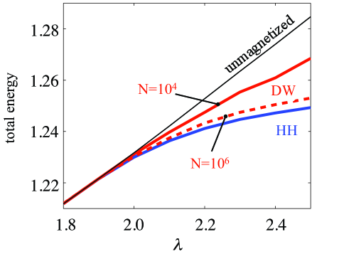
Figure 3: (Color online) Dimensionless total energy, $\varepsilon_{1}+\varepsilon_{2}$, shown as a function of interaction strength, $\lambda$, for an isotropic harmonic trap. DW indicates the energy of the domain wall state for $10^{4}$ atoms (solid) and $10^{6}$ atoms (dashed). HH denotes $\varepsilon_{1}+\varepsilon_{2}$ for the hedgehog state which is nearly identical for $10^{4}$ and $10^{6}$ atoms. Also shown (thin solid line, ‘unmagnetized’) is $\varepsilon_{1}$, defined in Eq.(44), which depends only on the total density profile.

Fig. 3 shows the energy $\bar{\varepsilon}^{HH}$ of the hedgehog state obtained by finding the function $m(r)$ which minimizes the hedgehog state energy. Fig. 4(a) shows the magnetization profile of the hedgehog state at two different interaction strengths. We find that the magnetization is suppressed in a small region around the trap center and vanishes at $r=0$. To understand the magnetization profile of the hedgehog near the trap center, we can focus just on the last two terms in Eq.(51). Taking a functional derivative with respect to $m(r)$ and setting it to zero then suggests that $m(r)\sim r^{2}$ at small $r$, so the energy density coming from the central region of the hedgehog is finite. Far from the center, we expect the magnetization to be small. These expectations are consistent with the magnetization profiles shown in Fig. 4(a).

IV.2 Isotropic trap: Domain wall state

For the domain wall state we have, as before,

$$\varepsilon_{1}\!\! = \!\!\frac{64}{3\pi}\int\!\!dr~{}r^{2}\left[\frac{6}{5}(\frac{n(r)}{2})^{5/3}\!\!+\!\!\frac{\lambda n^{2}(r)}{3\pi}\!+\!r^{2}n(r)\right].$$ (52)

For the magnetization dependent energy functional, we set $\alpha_{i}=1$ in the isotropic trap and choose ${{\vec{m}}}({{\bf{r}}})=m(r)\hat{z}$ for the domain wall. This is capable of describing a state with spin-$\uparrow$, say, at the trap center with spin-$\downarrow$ pushed away from the center, what we might call an ‘in-out’ domain wall. We find

$$\varepsilon_{2} = \frac{64}{3\pi}\int dr~{}r^{2}\left[A_{2}(r)m^{2}(r)+A_{4}(r)m^{4}(r)\right.$$ (53)

$$\!+\! \!\left.A_{6}(r)m^{6}(r)\!+\!\frac{n(r)}{144(3N)^{2/3}}\left(\!\frac{dm(r)}{dr}\!\right)^{2}\right]\!\!.$$

where, for $N_{\uparrow}=N_{\downarrow}$, we must satisfy the constraint $\int dr~{}r^{2}n(r)m(r)=0$.

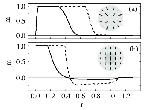
Figure 4: (a) Magnetization profiles for the hedgehog state at $\lambda=2.0$ (solid) and $\lambda=2.4$ (dashed). (b) Magnetisation profiles for the domain wall state at $\lambda=2.0$ (solid) and $\lambda=2.4$ (dashed). The profiles have been calculated for $10^{4}$ atoms in an isotropic trap. The hedgehog state has zero magnetization at the trap center while the domain wall state magnetization gets suppressed around the domain wall but remains nonzero at the trap center. Insets indicate the schematic magnetization plot of the hedgehog state and the domain wall state.

Fig. 3 shows the energy $\bar{\varepsilon}^{DW}$ of the domain wall state obtained by finding the function $m(r)$ which minimizes its energy subject to the zero magnetization constraint. We find that this domain wall state has a higher energy than the hedgehog state. Fig. 4(b) shows the magnetization profile of the domain wall state. As expected, the magnetization is suppressed in a small region around the domain wall but remains nonzero at the trap center.

IV.3 Cigar-shaped trap: Distorted hedgehog

If we consider a cylindrically symmetric (cigar-shaped) trap, we can look at an ansatz of the form

$$\vec{m}({\bf r})=m(\rho,z)\left(\frac{x}{\rho}\sin\psi,\frac{y}{\rho}\sin\psi,\cos\psi\right),$$ (54)

where $\rho=\sqrt{x^{2}+y^{2}}$ and $\psi\equiv\psi(\rho,z)$. For $\psi=\theta=\tan^{-1}(\rho/z)$ this reduces to the spherical hedgehog ansatz. Note that the direction of the magnetization on the Bloch sphere is unrelated to the location in real space. We could equally well have chosen, for instance,

$$\vec{m}({\bf r})=m(\rho,z)\left(\cos\psi,\frac{x}{\rho}\sin\psi,\frac{y}{\rho}\sin\psi\right).$$ (55)

With the choice of magnetization in Eq.(54), we have $|\vec{m}({{\bf{r}}})|^{2}=m^{2}(\rho,z)$, while

$$\alpha_{i}(\partial_{i}m_{j})(\partial_{i}m_{j})\!\!\! = \!\!\!\alpha_{\perp}(\partial_{\rho}m)^{2}\!+\!\alpha_{z}(\partial_{z}m)^{2}\!+\!\alpha_{\perp}\frac{m^{2}}{\rho^{2}}\sin^{2}\psi$$ (56)

$$+ m^{2}\left[\alpha_{\perp}(\partial_{\rho}\psi)^{2}+\alpha_{z}(\partial_{z}\psi)^{2}\right],$$

so the integral $\int d^{3}{{\bf{r}}}\to 2\pi\int dzd\rho\rho$. We can assume that $m$ is an even function of $z$ and that $\psi(\rho,-z)=\pi-\psi(\rho,z)$ (so that $\sin^{2}\psi(\rho,-z)=\sin^{2}\psi(\rho,z)$) to restrict the energy integration grid to just $z>0$. These conditions ensure that the total magnetization integrates to zero. The final expression for the energy can thus be recast, with $r\equiv\sqrt{\rho^{2}+z^{2}}$, as

$$\varepsilon_{1}\!\! = \!\!\frac{64}{3\pi}\!\int\!\!\!dr~{}r^{2}\!\!\left[\frac{6}{5}(\frac{n(r)}{2})^{5/3}\!\!+\!\!\frac{\lambda n^{2}(r)}{3\pi}\!+\!r^{2}n(r)\!\right]$$ (57)

$$\varepsilon_{2} = \frac{64}{3\pi}\!\!\int_{0}^{R_{max}}\!\!dz~{}\int_{0}^{\sqrt{r^{2}_{max}-z^{2}}}\!\!\!\!d\rho~{}\rho~{}F(\rho,z)$$ (58)

$$F(\rho,z) = A_{2}m^{2}+A_{4}m^{4}+A_{6}m^{6}$$ (59)

$$+ \frac{n}{144(3N)^{2/3}}\left\{\alpha_{\perp}\frac{m^{2}}{\rho^{2}}\sin^{2}\psi\right.$$

$$+ \alpha_{\perp}(\partial_{\rho}m)^{2}+\alpha_{z}(\partial_{z}m)^{2}$$

$$+ \left.m^{2}\left[\alpha_{\perp}(\partial_{\rho}\psi)^{2}+\alpha_{z}(\partial_{z}\psi)^{2}\right]\right\},$$

with $\psi(\rho=0,z)=0$ and $\psi(\rho,z=0)=\pi/2$ by symmetry. For notational simplicity, we have suppressed the coordinate labels on $n,m,\psi$ in the above functional.

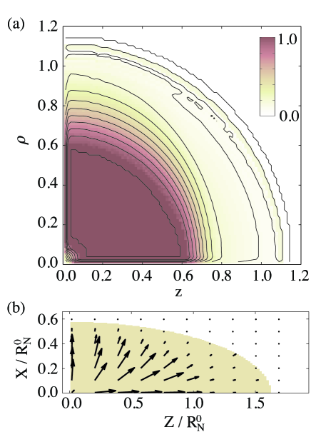
Figure 5: (Color online) Two-dimensional magnetisation profile for the distorted hedgehog showing breakdown of the LDA for the magnetization density for $10^{2}$ atoms in an anisotropic trap with $\lambda=2.4$, and $\alpha_{\perp}=2,\alpha_{z}=0.25$ ($\omega_{\perp}/\omega_{z}\approx 2.8$). (a) Plot of the magnitude of the magnetization $m(\rho,z)$ and equal-magnetization contours displayed in rescaled coordinates in which the trap potential is spherically symmetric. Colorbar to the right indicates the value of $m(\rho,z)$. We see that $m(\rho,z)$ is larger in magnitude for larger values of $\rho$ than it is for $z$, indicating that the surface tension makes it easier to change its value in the weak trapping direction. (b) $\vec{m}$ shown as a quiver plot indicating the magnitude and direction of the magnetization (plotted in coordinates where the trap anisotropy is explicitly shown). Shaded area indicates the region of the trap where the atom density is nonzero.

We find, numerically, that $\psi\approx\theta$, so in fact the ansatz simplifies to the form

$$\vec{m}({\bf r})=m(\rho,z)\left(\frac{x}{r},\frac{y}{r},\frac{z}{r}\right).$$ (60)

The main effect of going from the spherical to the cigar shaped trap is that the magnitude of the magnetization is no longer just dependent on the radial coordinate $r$. The magnetization however still points (in our rescaled coordinates) along the radial direction. The plot of the magnetization for $\lambda=2.4$ in the rescaled and in the original coordinates for a trap anisotropy corresponding to $\alpha_{\perp}=2,\alpha_{z}=0.25$ (a trap frequency ratio $\omega_{\perp}/\omega_{z}\approx 2.8$) is given in Fig. 5.

V Effect of dipolar interactions

Our results for the spin texture energetics and magnetization profiles have been obtained by neglecting the role of the long range magnetic dipole interaction between the fermions. The dipole interaction will add to the magnetic energy of atoms in the trap. In addition, it will lead to spatial variations of the magnetic field seen by atoms within the trap and, thus, cause tend to cause dephasing as atoms in different regions will precess at different rates. Such effects are known to be important in ⁸⁷Rb spinor Bose condensates vengalattore ; demler08 . In order to estimate the dipole interaction energy and the timescale of this dephasing, we have considered the spatial variations of the dipole field for the simple case of the spherical trap.

The expression for the precession frequency at distance $r$ from the center of the spherical trap is, for the hedgehog state,

$$\nu^{dip}_{HH}(r)\!\! \!\!=\!\! \!\!\frac{1}{h}\frac{\mu_{0}}{4\pi}\mu_{B}^{2}(\frac{2\sqrt{2}}{\pi\sqrt{3}})(\frac{\hbar}{M\Omega})^{-3/2}N^{1/2}$$ (61)

$$\!\!\times\!\! \!\!\!\int\!\!\frac{dr_{1}d\theta~{}r^{2}_{1}\sin\theta~{}m(r_{1})n(r_{1})}{(r^{2}+r^{2}_{1}-2rr_{1}\cos\theta)^{3/2}}F(r,r_{1},\theta),$$

$$\!\!F(r,r_{1},\theta)\!\! \!\!=\!\! \!\!\left[\cos\theta\!-\!3\frac{(r_{1}-r\cos\theta)(r_{1}\cos\theta-r)}{(r^{2}+r^{2}_{1}-2rr_{1}\cos\theta)}\right],$$ (62)

where $\mu_{B}\approx 9.27\times 10^{-24}J/T$ is the Bohr magneton, and $\mu_{0}=4\pi\times 10^{-7}N/A^{2}$ is the permeability of free space. Evaluating this, we find that the typical value of (and also the variation in) the precession frequency for $\lambda=2.5$, $N=10^{6}$, and $\Omega=2\pi(170{\rm Hz})$, is $\nu^{dip}_{HH}(^{6}{\rm Li})\approx 0.03{\rm Hz}$ and $\nu^{dip}_{HH}(^{40}{\rm K})\approx 0.6{\rm Hz}$. The energy associated with the dipole interactions is far smaller than our estimate of magnetic exchange energies, $\sim 500$Hz, arising from the s-wave contact interaction between fermions (in the interaction range where we expect ferromagnetism). At the same time, measurements of the typical atom lifetime, $\tau$, on the repulsive side of the Feshbach resonance indicate that $\tau\sim 10$ms for ⁴⁰K regal04 and $\tau\sim 100$ms for ⁶Li dieckmann02 ; bourdel03 . These are clearly much less than the variations in the precession period induced by spatial variations of the dipolar field as estimated above. Taken together, these estimates show that ignoring the effect of dipole interactions is a very good approximation in this system.

VI Conclusions

In conclusion, we have studied ferromagnetism and spin textures in ultracold atomic Fermi gases in the regime of strongly repulsive interactions using the LDA extended to include magnetization gradient corrections. Within the LDA at zero temperature, we have shown that the release energy of the gas, as well as its separate kinetic energy and interaction energy components, shows a sharp signature of the ferromagnetic transition. We have also shown that the atom loss rate via three-body collisions has a peak very close to the ferromagnetic transition and it provides yet another diagnostic of the transition into the ferromagnetic state. We have gone beyond the LDA by deriving a surface tension correction to the energy functional, which depends on atom number and the trap-geometry, and used it to study the energetics of various spin textures in a two-component trapped Fermi gas. For a spherically symmetric trap, we find that a hedgehog magnetization profile has lower energy than a domain-wall state. For large atom numbers, the small surface tension leads to a small energy difference between the two spin textures and the results are close to those of the LDA. In this case, the surface tension is responsible for selecting the hedgehog state as having the lowest energy but we have checked that it does not significantly change our results for the release energy and the atom loss rates. These continue to be useful, albeit indirect, diagnostics of the transition into the ferromagnetic state. For elongated clouds, we have shown that the surface tension term distorts the hedgehog states, in rescaled coordinates where the trap is isotropic, in such a manner that the magnitude of the magnetization changes more easily in the weak direction of the trap than would be expected on the basis of the LDA. Such a breakdown of the LDA is more apparent for smaller atom numbers. Finally, we have considered the effect of magnetic dipolar interactions on our results and find that it is a good approximation to ignore dipole interactions in this system.

The typical atom loss rate near the Feshbach resonance sets a constraint that the formation time for the ferromagnetic state will have to be on the order of tens of milliseconds for ⁴⁰K regal04 , and hundreds of milliseconds for ⁶Li dieckmann02 ; bourdel03 , in order for it to be observed. A direct way to probe the spin textures discussed here would be through high resolution in situ magnetometry as has been done for spinor Bose condensates stamperkurn06 . An experimental observation of ferromagnetism in trapped Fermi gases would provide impetus for future theoretical work on finite temperature effects and collective modes in the strongly interacting regime.