Gravity heats the Universe

Abstract

Structure in the Universe grew through gravitational instability from very smooth initial conditions. Energy conservation requires that the growing negative potential energy of these structures is balanced by an increase in kinetic energy. A fraction of this is converted into heat in the collisional gas of the intergalactic medium. Using a toy model of gravitational heating we attempt to link the growth of structure in the Universe and the average temperature of this gas. We find that the gas is rapidly heated from collapsing structures at around $z\,{\sim}\,10$, reaching a temperature ${>}\,10^{6}$K today, depending on some assumptions of our simplified model. Before that there was a cold era from $z\sim 100$ to $\sim 10$ in which the matter temperature is below that of the Cosmic Microwave Background.

Introduction.—It is well known that the temperature of the Cosmic Microwave Background is $T_{\gamma 0}=2.725\,$K, while the atomic matter today is typically orders of magnitude hotter than this. As the Universe expands the photon temperature drops so that $T(z)=T_{\gamma 0}(1+z)$, and Compton scattering couples the matter to the radiation until about $z\,{\simeq}\,100$, when it is allowed to cool adiabatically with $T\propto(1+z)^{2}$. In a perfectly smooth Universe with the same background cosmology as we observe today, the present temperature of the gas would be only about $20\,$mK Scott:2009sz .

However, the Intergalactic Medium (IGM) is composed of gas at a variety of temperatures (e.g. Valageas:2001wh ), ranging from ${\sim}\,10^{4}$K in dense clouds, up to ${>}\,10^{6}$K in the rarest inter-cloud gas. The reason that the gas is so hot is patently because the Universe contains structure. Our lumpy Universe generates thermal energy in a number of ways, but the simplest source is purely gravitational. The importance of gravitational heating for understanding the structure and evolution of galaxy clusters has been discussed by a number of authors (e.g. see Dekel:2007zy ; Khochfar:2007rp for recent examples). However, an explicit connection between gravity and heating of the IGM seems to have escaped notice in the literature. The gas is effectively heated from the growth of structure through gravitational instability, with the thermal energy coming from the increasingly negative energy of the growing potential wells.

The idea of gravitational shock heating of the IGM as a direct result of structure formation goes back at least to the ‘pancake’ model of the 1970s sz . This work was later extended using the ‘Zel’dovich approximation’ to follow the shock-heating of gas outside collapsed objects (see e.g. Nath:2001yd ), or in a related approach to use an extension of the Press-Schechter formalism to estimate the fraction of shocked gas Furlanetto:2003vk . Such numerical calculations allow for an investigation of the contributions of collapsed and shocked gas to temperature evolution of the IGM (see also Pen:1998eg ; Springel:2000bq ; Wang:2008zz ).

The details will of course be quite complicated, not least because starbursts and quasars provide photon and mechanical heating to the IGM in very non-linear and inhomogeneous processes. However, we will here focus only on gravity and aim to estimate the temperature of the IGM from the potential energy of the Universe, using a toy model to highlight the basic connection between gravitational and thermal energies. For our numerical work, we use the baryon density $\Omega_{\rm b}=0.045$, cold dark matter density $\Omega_{\rm c}=0.0255$, Hubble parameter $H_{0}=70\rm\,{\rm km}\,{\rm sec}^{-1}\,{\rm Mpc}^{-1}$, and the spectral index of initial fluctuations $n_{\rm s}=1$. To normalize the power spectrum we fix the matter variance in $8\,h^{-1}\,{\rm Mpc}$ spheres to $\sigma_{8}=0.9$. These values are consistent with the current best fit cosmological parameters Dunkley:2008ie .

Potential energy estimate from power spectrum.—The volume averaged gravitational potential energy (GPE) per unit mass as a function of redshift $z$ is Siegel:2005xu

$$W(z)=\frac{1}{2}\langle(1+\delta({\bf x},z))\phi({\bf x},z)\rangle\,,$$ (1)

where $\phi$ is the Newtonian potential, defined by the line element $ds^{2}=a^{2}\left[-(1+2\phi)d\tau+(1-2\phi)dx^{2}\right]$, and $\tau$ is conformal time. Using the Poisson equation $\nabla^{2}\phi=4\pi Ga^{2}\rho\,\delta$ and the definition of the correlation function

$$\xi({\bf r},z)\equiv\langle\delta({\bf x},z)\delta({\bf x}+{\bf r},z)\rangle=\frac{1}{(2\pi)^{3}}\int d^{3}{\bf k}\,{P}(k,z)e^{i\bf{k\cdot r}}\,,$$ (2)

where $P(k,z)\equiv|\delta(k,z)|^{2}$, the Newtonian potential energy is

$$W(z)=-\int\frac{dk}{k}\Delta_{\rm W}^{2}(k,z)\,,$$ (3)

and with the dimensionless gravitational power

$$\Delta_{\rm W}^{2}(k,z)\equiv\frac{3H_{0}^{2}\Omega_{\rm m,0}(1+z)}{8\pi^{2}}P(k,z)\,k\,.$$ (4)

This can also be obtained from the definition in Peebles Peebles , $W=-\frac{1}{2}G\rho_{\rm m}a^{2}\int d^{3}{\bf r}\,\xi({\bf r},z)/{\bf r}=-2\pi G\rho_{\rm m}\,J_{2}$, where $J_{2}=\int dkP(k,z)/(2\pi^{2})$. In Fig. 1 we show $(1+z)\Delta_{\rm W}^{2}(k,z)$ for our cosmological model at $z=0,1,10$ and $100$. The peak of the gravitational energy contribution occurs at a comoving scale of $\sim 10$ Mpc.

In the matter dominated era ($z\gtrsim 1$) the quantity $(1+z)\Delta_{\rm W}^{2}(k,z)$ remains roughly constant, since the growth factor, given by $D(z)=\delta_{\rm m}(z)/\delta_{\rm m}(z=0)$ , scales as $(1+z)^{-1}$. At lower $z$, in the dark energy dominated era, the growth of structure is significantly suppressed due to the increasing expansion rate – this slow down has recently been detected in observations of galaxy clusters Vikhlinin:2008ym .

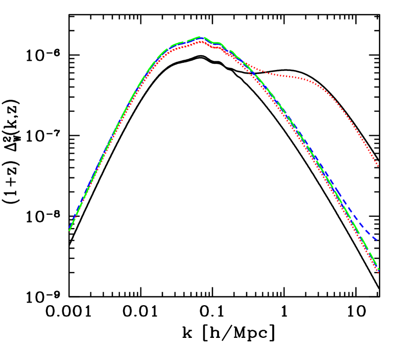
Figure 1: Normalized gravitational potential as a function of scale at $z=0$ (solid), 1 (dotted), 10 (short-dashed) and 100 (long-dashed). The corresponding curves with additional small-scale power are non-linear corrections from the HALOFIT code Smith .

In order to estimate the IGM temperature $T_{\rm gas}(z)$ one can suppose that the GPE is equal to the average kinetic density energy of baryonic matter. Therefore, one could set $\rho_{\rm m}W=\rho_{\rm b}kT/m_{\rm H}$, where $k$ is Boltzmann’s constant, $m_{\rm H}$ the mass of hydrogen (neglecting helium for simplicity) and $\rho_{\rm m}$, $\rho_{\rm b}$ are the energy densities of matter and baryons respectively. We show the results of this calculation in Fig. 2, along with $T(z)$ from the recombination code RECFAST Seager:1999km ; Wong:2007ym , which assumes the matter distribution is perfectly smooth and cools adiabatically. One finds an average temperature of $\sim 10^{8}$ K at $z=0$, and the ‘gravitational temperature’ exceeds the RECFAST value for $z<1000$.

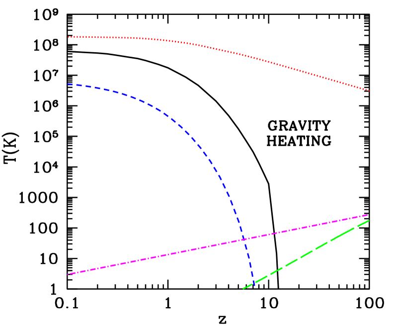
Figure 2: Evolution of $T_{\rm gas}(z)$ for linear theory (dotted curve), non-linear theory with a cut-off scale (solid) and halo number density (short-dashed) . We also show the baryonic temperature evolution from the RECFAST code Seager:1999km ; Wong:2007ym (long-dashed) and the CMB temperature (dot-dashed).

Clearly, this linear calculation over-predicts the temperature. The reason for this is that gravitational shock-heating is associated with the collapse of non-linear objects and shell-crossing. The linear GPE is largest on scales of $\sim 10$ Mpc, which are only just going non-linear at $z=0$. Linear scales are associated with smooth bulk flows, and hence there is no mechanism for the gas to be heated. To be more realistic, we should only include the total GPE coming from non-linear scales at a given redshift. In this regime, setting $\rho_{\rm m}W=\rho_{\rm b}kT/m_{\rm H}$ implicitly assumes that the damped outgoing shock waves from collapsed objects efficiently (and instantaneously) heat the IGM.

Since the linear power spectrum becomes becomes inaccurate on small-scales, we include non-linear corrections to $P(k,z)$ from the the HALOFIT code Smith . These corrections are shown in Fig. 1, and result in an increase of small-scale power. In order to estimate the cut-off scale at which perturbations are going non-linear, we compute the value $R_{\rm NL}$ at which the RMS mass variance

$$\delta_{\rm R}^{2}(z)=\int\frac{dk}{k}\Delta^{2}(k,z)W^{2}(kR)\,,$$ (5)

is equal to unity. Here $W(x)$ is the window function associated with a spherical top-hat, and $\Delta^{2}(k,z)=k^{3}P(k,z)/(2\pi^{2})$ is the dimensionless power spectrum. We then perform the integral only above $k_{\rm NL}=2\pi/R_{\rm NL}$. The results of this computation are shown in Fig. 2 – one finds a smaller temperature at $z=0$, and a much faster decrease with redshift. This is due to $k_{\rm NL}$ shifting to smaller-scales for increasing $z$, so less GPE contributes to the heating.

Halo number density estimate.—We can also estimate the gravitational energy in a different way by just considering viralized objects. Virialization occurs at higher over-densities than those discussed previously – in a flat Einstein-de-Sitter model linear theory predicts a spherical top-hat will break away from the expansion at a mass fluctuation of $\delta=1.063$, collapse at $\delta=1.686$, but virialize at $\delta=1.59$ (see e.g. padmanabhan ). We use the Press-Schechter mass function ps to estimate the number density of viralized objects

$$\frac{dn}{dM}(z,M)=\sqrt{\frac{2}{\pi}}\frac{\rho_{\rm m}(t_{0})}{M^{2}}\nu e^{-\nu^{2}/2}\left[-\frac{d\ln\sigma_{\rm M}(z=0)}{d\ln R}\right]\,,$$ (6)

where $\nu\equiv\delta_{\rm c}/\left[D(z)\sigma_{\rm M}(z=0)\right]$, the critical threshold $\delta_{\rm c}=1.686$, the mass enclosing a sphere of radius $R$ is $M=4\pi\rho_{\rm m}(t_{0})R^{3}/3$ and the growth function is normalized to unity today. The growth function can be computed from

$$D(a)=\frac{5\Omega_{\rm m,0}}{2}\frac{H(a)}{H_{0}}\int^{a}_{0}\frac{da^{\prime}}{(a^{\prime}H(a^{\prime})/H_{0})^{3}}\,,$$ (7)

where the scale-factor $a=1/(1+z)$ and $H(a)$ is the Hubble rate.

In order to compute the gravitational energy we can use the virial theorem, $W=-2K$, where the kinetic energy per unit volume is $K=k\langle T_{\rm vir}\rangle M_{\rm tot}$. The mass averaged virial temperature is defined as

$$\langle T_{\rm vir}\rangle=\frac{1}{M_{\rm tot}}\int^{\infty}_{0}T_{\rm vir}M\frac{dn}{dM}dM$$ (8)

with $M_{\rm tot}=\int^{\infty}_{0}M\frac{dn}{dM}dM$. We use the virial temperature normalization for a conventional cosmology in Pierpaoli:2000ip , with $T_{\rm vir}({\rm K})=5\times 10^{-23}\,(M/{\rm kg})^{2/3}(1+z)$.

We again assume that outgoing shock waves effectively share out the GPE among all the particles in the Universe, not just those in virialized structures. Hence one can equate $k\langle T_{\rm vir}\rangle M_{\rm tot}=\rho_{\rm b}kT$ to obtain the evolution of $T(z)$. This is shown in Fig. 2 – the redshift evolution has a similar profile to the non-linear power spectrum estimate (with a cut-off scale $R_{\rm NL}$), although the temperature is approximately an order of magnitude lower. One can see that effectively these two calculations are very similar, with mainly just a different choice of cut-off scale.

Gas cooling.—So far, we have assumed that the IGM is heated without taking into account cooling processes in the gas. We can expect this to be a reasonable estimate as long as the cooling time-scale is longer than the Hubble time $H^{-1}$. Assuming the cooling is dominated by thermal bremsstrahlung we show the ratio of cooling to Hubble time in Fig. 3. For our model of IGM heating from only collapsed objects, we find the cooling time becomes less than the Hubble time around $z\,{\sim}\,10$. At this point the baryonic matter in the IGM will begin to heat from its adiabatically cooled value of ${\sim}\,3\,$K. The CMB temperature is ${\sim}\,30\,$K at $z\,{\sim}\,10$, so it appears there is an epoch from $z\,{\sim}\,10$–100 when the matter is actually colder. Since the IGM is outside collapsed regions and thus taking part in the Hubble expansion, it will also continue to cool adiabatically – including this additional effect in our computations leads to a reduction in temperature by a factor of 2–3 at $z=0$.

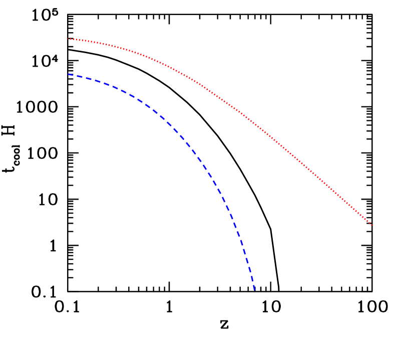
Figure 3: Ratio of cooling time to Hubble time. Lines are labelled the same as in Fig. 2.

Conclusions.—Since the Universe is lumpy, it is necessarily hot. A simplistic picture is that the temperature of the IGM comes from energy balance with a fraction of the gravitational energy that is building up through gravitational instability. Virliaization of structures require that about half of the potential energy is lost to the ‘environment’, here meaning that the dark and baryonic matter acquire kinetic energy. When shell-crossing occurs kinetic energy is converted into thermal energy in the collisional material, the IGM gas. We have shown that this picture leads to an IGM which is significantly colder than the CMB until gravitational heating takes over at $z\,{\sim}\,10$.

Things became rapidly more complicated just after this era. An accurate calculation of the heating process would require solving for the inhomogeneous growth of structure, including hydrodynamic effects, as well as cooling processes. In addition, reionization of the Universe appears also to happen at $z\,{\sim}\,10$ and so photon sources, electromagnetic interactions and radiative transfer need to be considered in order to fully understand the IGM today. Many astrophysics theorists are working hard on just these problems.

Acknowledgments.—This research was supported by the Natural Sciences and Engineering Research Council of Canada. We thank the many colleagues with whom we have had fruitful discussions on this topic, in particular Alan Duffy, Kris Sigurdson, Martin White and Jim Zibin.

References

- (1) D. Scott and A. Moss, (2009) [arXiv:0902.3438].
- (2) P. Valageas, R. Schaeffer and J. Silk, Astron. Astrophys. 388, (2002) 741 [astro-ph/0112273].
- (3) A. Dekel and Y. Birnboim, MNRAS 383, (2008) 119 [arXiv:0707.1214]
- (4) S. Khochfar and J. P. Ostriker, Astrophys. J. 680, (2008) 54 [arXiv:0704.2418].
- (5) R. A. Sunyaev and Y. B. Zel’dovich, Astron. Astrophys. 20, (1972) 189.
- (6) B. B. Nath and J. Silk, MNRAS 327, (2001) 5 [astro-ph/0107394].
- (7) S. Furlanetto and A. Loeb, Astrophys. J. 611, (2004) 642 [astro-ph/0312435].
- (8) U. Pen, Astrophys. J. 510, (1999) 1 [astro-ph/9811045].
- (9) P. Wang and T. Abel, Astrophys. J. 672, (2008) 752.
- (10) V. Springel, M. White and L. Hernquist, (2000) [astro-ph/0008133].
- (11) J. Dunkley et al, Astrophys. J.Ṡupp. 180, (2009) 306 [arXiv:0803.0586].
- (12) E. R. Siegel and J. N. Fry, Astrophys. J. 628, (2005) 1 [astro-ph/0504421].
- (13) P. J. E. Peebles, Physical Cosmology, Princeton University Press (1971) .
- (14) R. E. Smith et al, MNRAS 341, (2003) 1311 [astro-ph/0207664].
- (15) A. Vikhlinin et al, (2008) [arXiv:0812.270].
- (16) S. Seager, D. D. Sasselov and D. Scott, Astrophys. J.Ṡupp. 128, (2000) 407 [astro-ph/9912182].
- (17) W. Y. Wong, A. Moss and D. Scott, MNRAS 386, (2008) 1023 [arXiv:0711.1357].
- (18) T. Padmanabhan, Theoretical Astrophysics: Galaxies and Cosmology, Cambridge University Press (2002) .
- (19) W. H. Press and P. Schechter, Astrophys. J. 187, (1974 452.
- (20) E. Pierpaoi, D. Scott and M. White, MNRAS 325, (2001) 77 [astro-ph/0010039].