Headway oscillations and phase transitions for diffusing particles with increased velocity

Abstract

An asymmetric exclusion process with $N$ particles on $L$ sites is considered where particles can move one or two sites per infinitesimal time-step. An exact analysis for $N=2$ and a mean-field theory in comparison with simulations show even/odd oscillations in the headway distribution of particles. Oscillations become maximal if particles try to move as far as possible with regard to their maximum velocity and particle exclusion. A phase transition separates two density profiles around a generated perturbation that plays the role of a defect. The matrix-product ansatz is generalized to obtain the exact solution for finite $N$ and $L$. Thermodynamically, the headway distribution yields the mean-field result as $N^{-1}\rightarrow 0$ while it is not described generally by a product measure.

1 Introduction

Driven-diffusive systems such as the asymmetric simple exclusion process (ASEP) have been extensively used to model traffic flow phenomena [1]. It is defined on a one-dimensional lattice in which particles can move only in one direction with respect to the exclusion rule which implies that at most one particle can stay at a single site. From a theorist’s point of view these models are especially interesting in respect of phase transitions, such as a jamming and condensation transitions and their solvability at least for the steady state. Usually, the rather sophisticated models that claim to reproducing real traffic features are not available for exact mathematical descriptions. The more important are the minimalist models that lead to an understanding of the underlying physics. The ASEP in one dimension with periodic boundary conditions is fairly simple and has a uniform stationary measure [2]. There are, however, some generalizations of the ASEP with periodic boundary conditions that lead to phase transitions. An example is the ASEP with a single defect particle that can itself move forward on empty sites and can be overtaken by normal particles [16]. The defect can be thought of as a truck that moves in an environment of cars [2]. Another example is particle disorder: If any of the particles has an individual fixed hopping rate one might observe a phase transition from a fluid into a condensed phase [7]. Finally phase transitions have been studied in asymmetric exclusion models in which the hopping rate depends on the empty space ahead. These models can often be related to the zero-range process and the interactions are normally long-ranged when condensation transitions appear [8, 9]. The ZRP itself allows for an arbitrary number of particles per site and the single-particle hopping-rate depends only on the occupation on the departure site [9]. This has been generalized to models in which more than one particle can move. A condition on the hopping rates has been derived for the steady state to take a simple factorized form [10].

In the following section we define a simple traffic model, which is a generalization of the ASEP in the sense that particles can move one or two sites per infinitesimal time-step. We find that the system leads to oscillations in the distribution of head-ways which become maximal when it is impossible to move only one site if there are more empty sites available. Here the system evolves in special regions of the configuration space that gives rise to a phase transition. Although it is a very simple conserving process on a ring with one species of particles, no overtaking and short-range interactions it is capable to produce a phase transition and has a non-trivial steady state that is obtained exactly. We investigated also the process with parallel update and found the matrix-product stationary state, see [5].

2 The general process

The general process we are going to investigate is defined on a one-dimensional lattice with $L$ sites, enumerated $l=1,2,\dots,L$. Each site $l$ may either be occupied by one particle ($\tau_{l}=1$) or it may be empty ($\tau_{l}=0$). We impose periodic boundary conditions and let the system evolve in continuous time. Particles can move one or two sites to the right according to the following rules:

$$100 \rightarrow 010,\quad{\rm at\;rate}\;p_{1},$$

$$\rightarrow 001,\quad{\rm at\;rate}\;p_{2},$$

$$101 \rightarrow 011,\quad{\rm at\;rate}\;\beta.$$ (1)

The parallel-update version of this process has been considered in [19]. Note that the total number of particles $N$ is fixed due to the allowed transitions and boundary conditions. Some simple cases are already known: For example $p_{1}=\beta$ was studied in [23] and turned out to have a uniform stationary state. For $p_{2}=0$ one finds [23, 21] that the weights (for $\beta>0$) are of the pair-factorized form: $P(\tau_{1},\tau_{2},\dots,\tau_{L})=\prod_{l=1}^{L}t(\tau_{i},\tau_{i+1})$ with some simple two-site factors $t(\tau_{i},\tau_{i+1})$. A mapping onto a mass- transport model shows that these are the only cases with factorized steady state (see section 3.3).

2.1 Two-particle study

In the following we consider (2) with only two particles on a ring. The quantity of interest is the un-normalized steady-state weight $f(m,n)$, denoting that one particle is followed by $m$ and the other by $n$ holes. Analysis of the master equation shows that these weights obey the following second-order recursion relation

$$f(m,n)=\omega_{L}(p_{1})f(m-1,n)+p_{2}f(m-2,n),\;{\rm for}\;m\geq n\;{\rm and}\;m+n=L-2\geq 3,$$ (2)

with the piecewise defined function

$$\omega_{L}(p_{1}) =\cases{p_{1},&for $L$ even,\\ 1,&for $L$ odd.}$$ (3)

One rate can be chosen as 1 and it is convenient to set $p_{1}=1$ to get rid of the even/odd dependence of the lattice size. Concluding we take for the study of the two-particle case $\omega_{L}(p_{1}=1)\equiv 1$. In terms of the functions

$$y_{n}:=\left(\frac{1+\sqrt{1+4p_{2}}}{2}\right)^{n}+\left(\frac{1-\sqrt{1+4p_{2}}}{2}\right)^{n}$$ (4)

the solution of (2) (for $m\geq n$ and $m\geq 1$) is

$$f(m,n) = \frac{\beta y_{m+n}+(2p_{2}+1-\beta)y_{m+n-1}}{1+4p_{2}}+(-1)^{n-1}\frac{(1-\beta)p_{2}^{n}y_{m-n}}{1+4p_{2}}.$$ (5)

One sees that the first term only depends on $n+m$ and therefore it is constant for given system size. The second term has a pre-factor $(-1)^{n-1}$ which indicates that in general there are oscillations. Thus the weights $f(m,n)$ depend on the parity of $n$. The probability for a certain configuration with two particles is given by $P(m,n)=Z_{m+n+2,2}^{-1}f(m,n)$, where for system size $L$ the normalization $Z_{L,2}=\sum_{m=0}^{L-2}f(m,L-2-m)$ is:

$$Z_{L+1,2}=\left[\frac{\beta L}{1+4p_{2}}-\frac{2(1-\beta)(2p_{2}+1)}{(1+4p_{2})^{2}}\right]y_{L-1}+\left[\frac{(2p_{2}+1-\beta)L}{1+4p_{2}}-\frac{2p_{2}(1-\beta)}{(1+4p_{2})^{2}}\right]y_{L-2}.$$ (6)

One might think that the feature of oscillations comes from the presence of a finite number of particles, so we investigate the thermodynamic limit within a mean-field theory.

2.2 Mean-Field Theory

To take into account correlations between consecutive particles we write down an improved mean-field theory. The quantity of interest is the probability $P(m)$ to find a headway of $m$ empty sites in front of a particle. In the context of traffic-flow models this is referred to as car-oriented mean-field theory (COMF) [4]. The stationary equations read:

$$(c+p_{2}s)P(0) = \beta P(1)+p_{2}P(2),$$

$$(c+p_{2}s+\beta)P(1) = cP(0)+p_{1}P(2)+p_{2}P(3),$$ (7)

$$(c+p_{2}s+p_{1}+p_{2})P(m) = p_{2}sP(m-2)+cP(m-1)+p_{1}P(m+1)+p_{2}P(m+2),$$

$${\rm for}\;m\geq 2,$$

with the short-hand notations

$$s:=1-P(0)-P(1)\;{\rm and}\;c:=\beta P(1)+p_{1}s.$$ (8)

We now introduce the generating function

$$Q(z)=\sum\limits_{m=0}^{\infty}P(m)z^{m}.$$ (9)

Summing up $P(m)z^{m}$ for $m=0\dots\infty$ leads to a rational expression for $Q(z)$ from which a singularity at $z=1$ can be removed. One obtains

$$Q(z)=\frac{(\beta-p_{1}-p_{2})P(1)z^{2}-wz-p_{2}P(0)}{p_{2}sz^{3}+(c+p_{2}s)z^{2}-(p_{1}+p_{2})z-p_{2}},$$ (10)

with $w:=(p_{1}+p_{2})P(0)+p_{2}P(1)$. A useful check of this equation is $Q(0)=P(0)$ and $Q(1)=1$. The density $\rho$ in the corresponding asymmetric exclusion process is

$$\partial_{z}(zQ(z))|_{z=1}=\sum\limits_{m=0}^{\infty}(m+1)P(m)=\rho^{-1}.$$ (11)

This gives $P(1)$ in terms of $P(0)$ and $\rho$:

$$P(1)=\frac{\left[2p_{2}(1+\rho)+p_{1}\right]P(0)-(4p_{2}+p_{1})\rho}{(\beta-p_{1})(1-\rho)-2p_{2}}.$$ (12)

The remaining probabilities can be obtained from $Q(z)$. The flow-density relation is $J(\rho)=\rho(c+2p_{2}s)$.

However at this stage already one equation is missing. One needs an additional relation between $P(1)$ and $P(0)$ to be able to express everything in terms of the density only. In fact, the missing relation can be extracted from the generating function. Writing the numerator of $Q(z)$ in terms of its zeros $z_{0}^{\pm}$ gives $(\beta-p_{1}-p_{2})P(1)(z-z_{0}^{+})(z-z_{0}^{-})$. The singularity in the unit circle then has to be removed by $z_{0}^{+}$ or $z_{0}^{-}$ for $Q(z)$ to be analytic [4]. This leads to the missing relation between $P(1)$ and $P(0)$ [15].

We restrict ourselves here to the case where the coefficient of $z^{2}$ in the numerator of $Q(z)$ vanishes, since there the mean-field predictions can be written in a very compact form and the main-features that we want to display are contained. Consider $\beta=p_{1}+p_{2}$: a headway’s total rate of change is independent of its length. The condition is weaker than the condition for a factorized state (every configuration is equally probable if $p_{1}=\beta$). Substituting this into (10) and demanding that the denominator has the same zero as the numerator gives the missing relation:

$$p_{2}P(1)^{2}=p_{1}P(0)\left(P(0)[1-P(0)]-P(1)\right).$$ (13)

For $Q(z)$ one gets the simple expression

$$Q(z)=\frac{pP(0)A^{2}}{pA^{2}-pAz-z^{2}},$$ (14)

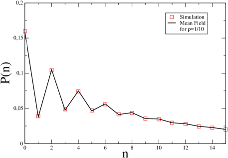
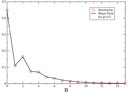
with $A:=P(0)/P(1)$ and $p:=p_{1}/p_{2}$, which can nicely be expanded to obtain $P(m)$. Figure 1 shows the mean-field distribution for two different choices of parameters in comparison with computer simulations. While $P(n)$ decays rapidly, one sees the characteristic even/odd oscillations which are well reproduced by mean field.

Figure 1: Headway distribution $P(n)$ from a computer simulation with $L=1000$ in comparison with mean field for $p_{2}=1$. Left: $p_{1}=0.1$, $\beta=1.1$ and $\rho=0.1$. Right: $p_{1}=0.2$, $\beta=1.2$ and $\rho=1/3$.

2.2.1 The Fibonacci case

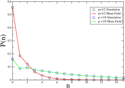
Remarkable is the case $\beta=p_{1}+p_{2}=2$ with $p_{1}=p_{2}=1$. Then the probabilities $P(m)$ are given by the Fibonacci numbers:

$$P(m)=P(0)\left(\frac{P(1)}{P(0)}\right)^{m}F_{m+1}.$$ (15)

Here one obtains from (13): $P(1)/P(0)=(\sqrt{5-4P(0)}-1)/2$ and relating $P(0)$ to the density gives

$$P(0)=\frac{\rho}{(1+\rho)^{2}}\frac{5+4\rho-\sqrt{5-4\rho^{2}}}{2}.\\$$ (16)

Figure 2 shows the headway distribution for the Fibonacci case.

Figure 2: Headway distribution $P(n)$ from mean-field for the Fibonacci case $p_{1}=p_{2}=1$ and $\beta=2$ for $\rho=1/8$ and $1/2$ compared with computer simulations.

2.2.2 The choice $p_{1}=0$

In (10) one sees that also $P(1)=0$ reduces the numerators degree to one. It has a zero at $z=-p_{2}(p_{1}+p_{2})^{-1}$. We are interested in $p_{2}>0$, so take $p_{2}=1$ without loss generality. Demanding that the denominator has the same zero yields (as the only physical solution) $p_{1}=0$. The generating function reduces to $P(0)\left(1+(1-P(0))z^{2}+(1-P(0))^{2}z^{4}+\dots)\right)$. So $P(1)=0$ has the consequence that $P(2n+1)$ vanishes generally and the process is realized only on the even sublattice in mean field. The relation to the density is

$$P(0)=\frac{2\rho}{1+\rho},$$ (17)

and the flow simply reads

$$J(\rho)=2\rho\left[1-P(0)\right]=\frac{2\rho(1-\rho)}{1+\rho}.$$ (18)

These results are completely equivalent to the usual ASEP where now particles always move two sites and the density is appropriately rescaled.

3 Maximal Oscillations: The choice $p_{1}=0$

We consider the process

$$100 \rightarrow 001,\quad{\rm at\;rate}\;1,$$

$$101 \rightarrow 011,\quad{\rm at\;rate}\;\beta,$$ (19)

Physically, this is the case where every particle tries to move as far as possible with regard to his maximum velocity. This is the limit in which the oscillations in the form of even/odd effects become maximal. This type of process evolves into special regions of the configuration space. We try to find the full solution for finite $N$ and $L$ from the matrix-product ansatz.

3.1 Unified solution for finite number of particles and sites

The state of the periodic system can be expressed by the sequence of headway: $\{n_{1},\dots,n_{N}\}$. We look for a product state of the form:

$$F(n_{1},n_{2},\dots,n_{N})={\rm Tr}\prod\limits_{\mu=1}^{N}\mathcal{G}_{n_{\mu}},$$ (20)

where $\mathcal{G}_{n_{i}}$ is an operator representing particle $\mu$ followed by $n_{\mu}$ holes. It turns out that this ansatz (with a certain trace-like operation Tr$=$tr$||.||$ to be specified below) yields the correct steady state, provided that the involved operators fulfill the following quadratic algebra:

$$\mathcal{G}_{2i}\mathcal{G}_{1} = \mathcal{G}_{2i+1},$$ (21)

$$\mathcal{G}_{2i+1}\mathcal{G}_{2j+2}-\mathcal{G}_{2i+1}\mathcal{G}_{2j} = 0,$$ (22)

$$\mathcal{G}_{2i}\mathcal{G}_{2j+2}-\mathcal{G}_{2i}\mathcal{G}_{2j} = \beta\mathcal{G}_{2i+2j+2},$$ (23)

$$\mathcal{G}_{2i}\mathcal{G}_{2j+3}-\mathcal{G}_{2i}\mathcal{G}_{2j+1} = \beta\mathcal{G}_{2i+2j+3},$$ (24)

$$\mathcal{G}_{2i+1}\mathcal{G}_{2j+1} = 0,\qquad\quad\quad{\rm for}\;i,j\geq 0.$$ (25)

We just note here that this can be proven by use of the canceling-mechanism [15]. The corresponding tagged operators read:

$$\bar{\mathcal{G}}_{0} = \mathcal{G}_{0}-\beta\mbox{$1\!\!1$},$$ (26)

$$\bar{\mathcal{G}}_{2(i+1)} = \mathcal{G}_{2(i+1)}+\mathcal{G}_{2i},$$ (27)

$$\bar{\mathcal{G}}_{1} = \mathcal{G}_{1},$$ (28)

$$\bar{\mathcal{G}}_{2i+3} = \mathcal{G}_{2i+3}+\mathcal{G}_{2i+1}.$$ (29)

It is important to emphasize that (25) implies that the system can not support more than one odd gap. This can be understood directly from the dynamical rules (3). The fact that the transition $100\rightarrow 010$ is forbidden ($p_{1}=0$) has the consequence that the number of odd gaps decreases with time: A configuration $\mathcal{C}(\dots 1$[any odd number of 0s]$101|\dots$) moves with conditional probability $\beta$ into a configuration with two odd-valued gaps less (creation of even gaps), while odd gaps can not emerge. These processes appear until there remain either no more odd gaps ($L-N$ even) or exactly one odd gap ($L-N$ odd). In the latter case this means physically that the probability for odd gaps is of order $1/N$ and thus tends thermodynamically to zero as predicted by mean-field.

One has to be careful with a unified description for an arbitrary number of odd gaps in the system. The operators $\mathcal{G}$ are mathematical objects that can in our case be written as matrices whose components are itself matrices (compare [12, 5]). Thus it is not obvious how to generalize the trace operation. The straight-forward generalization to a sum of the traces of the matrices on the main diagonal can here not be applied: This trace operation and therewith the weight for certain configurations can incorrectly give zero. The problem of the trace operation for periodic systems has previously be pointed out [6]. The matrix relation (25) implies that $(\mathcal{G}_{2i+1})^{2}=0$ for all $i$. For a unified description the operators $\mathcal{G}_{2i+1}$ had to be non-vanishing nilpotent matrices. However for this equation to hold all the eigenvalues of $\mathcal{G}_{2i+1}$ must be equal to zero. Therefore also tr $\mathcal{G}_{2i+1}=0$ which implies for example through relation (21) that also tr $\mathcal{G}_{2i}\mathcal{U}_{1}=0$ which is untrue. Now this argument can be used successively to see that for every $N$ the straight-forward trace operation can not be applied. First, the algebra (21-25) can be simplified:

$$\mathcal{G}_{2i+1}=\mathcal{E}^{i}\mathcal{A}\;{\rm and}\;\mathcal{G}_{2i}=\beta\mathcal{E}^{i}\mathcal{D}$$ (30)

with new operators $\mathcal{E}$ and $\mathcal{D}$. Then (21-25) reduces to

$$\mathcal{D}\mathcal{E} = \mathcal{D}+\mathcal{E},$$ (31)

$$A\mathcal{E} = \mathcal{A},$$ (32)

$$\beta\mathcal{D}\mathcal{A} = \mathcal{A},$$ (33)

$$\mathcal{A}^{2} = 0.$$ (34)

Introduce the two by two matrices $\mbox{$1\!\!1$}=|1\rangle\langle 1|+|2\rangle\langle 2|$, $\mbox{$2\!\!2$}=|1\rangle\langle 2|$ and let further be $\mathcal{E}=E\otimes\mbox{$1\!\!1$}$, $\mathcal{D}=D\otimes\mbox{$1\!\!1$}$, and $\mathcal{A}=A\otimes\mbox{$2\!\!2$}$, with matrices $E$, $D$, and $A$. Then one can interpret the trace operation in (20) as $F(n_{1},n_{2},\dots,n_{N})={\rm tr}||\prod_{\mu=1}^{N}\mathcal{G}_{n_{\mu}}||,$ with the help of the matrix norm $||M||=$ max${}_{i,j}m_{ij}$ to obtain always the correct weights. A different method is for example a parity-dependent matrix representation [15]. However beyond the question of how to obtain the correct matrix element it is most convenient to consider both cases separately.

3.2 Expectation values and phase transition

For even number of holes only even gaps occur in the stationary state. With the particles always making two steps $(100\rightarrow 001)$ the stationary process is completely equivalent to the ASEP. All configurations with even-length gaps have the same stationary weight (the matrices $\mathcal{D}$ and $\mathcal{E}$ are sufficient to describe the steady state and can be chosen as numbers). For the normalization we find

$$Z_{L,N}=\frac{L(L-M-1)!}{N!M!}\delta_{L-N,2M}.$$ (35)

This is easily interpreted combinatorially: For the first particle one has $L$ possible ways to place it on the lattice. One can then think of distributing $N-1$ particles and $M$ hole pairs into $N+M-1$ boxes to obtain the above expression. The flow (from site $i$) is the expectation value

$$J=\langle\tau_{i}(1-\tau_{i+1})(1-\tau_{i+2})\rangle+\beta\langle\tau_{i}(1-\tau_{i+1})\tau_{i+2})\rangle=\langle\tau_{i}\rangle-\langle\tau_{i}\tau_{i+1}\rangle.$$ (36)

With $\langle\tau_{i}\rangle=\frac{N}{L}$ and $\langle\tau_{i}\tau_{i+1}\rangle=N/L\cdot(N-1)/(L-M-1)$ this yields asymptotically the mean-field current (18). The exact form of the velocity for finite system size reads

$$v=2\frac{1-\rho}{1+\rho}\left(1+\frac{2}{L+N}+\dots+\frac{2^{n}}{(L+N)^{n}}+\dots\right).$$ (37)

For odd number of holes exactly one odd gap occurs in the steady state. If one considers only stationary configurations the relation (34) becomes redundant. The non-vanishing steady-state weights from (20) can simply be written as

$$F(2n_{1},2n_{2},\dots,2n_{N}+1)={\rm tr}\;\left[\prod\limits_{\mu=1}^{N-1}E^{n_{\mu}}D\right]E^{n_{N}}A.$$ (38)

Here we referred to the particle with the odd gap in front as particle $N$. Due to the translational invariance this can be done without loss of generality. The underlying algebra reduces to

$$DE=D+E,\quad AE=A,\quad{\rm and}\;\beta DA=A.$$ (39)

This is the algebra for the ASEP with a single defect particle [16] for the case $\alpha=1$. This process is defined by transitions $10\rightarrow 01$ at rate 1, $20\rightarrow 02$ at rate $\alpha=1$ and $12\rightarrow 21$ at rate $\beta$. In fact, the stationary states of both processes are completely equivalent. In our process even gaps of length $2n$ are mapped onto gaps of length $n$ in the defect ASEP (00 becomes 0). Now consider the single odd gap with the particle to its right. It can be written in the form 00 00 $\dots$ 01. Again 00 is mapped onto 0 and 01 becomes the defect 2. One can check that under this mapping indeed (3) recovers the transitions of the defect ASEP. Note that $\alpha=1$ takes care of the (physically reasonable) fact that in our process particles with an even or odd gap to their left move forward at the same rate.

As for the defect ASEP the partition function can be calculated:

$$Z_{L,N}=\frac{L}{N}{N+M\choose N-1}\sum\limits_{m=1}^{\infty}m{N+M-1\choose N-m}\left(\frac{1-\beta}{\beta}\right)^{m-1}\delta_{L-N,2M+1}$$ (40)

From this expression correlation functions can be derived as above. It turns out that the flow is related to the normalization by

$$J=2\frac{N}{L-2}\frac{Z_{L-2,N}}{Z_{L,N}}+\beta\frac{L-N}{L-1}\frac{Z_{L-1,N-1}}{Z_{L,N}}.$$ (41)

We have calculated the finite size expansion for the velocity in the case $\beta=1$ and obtained

$$v=2\frac{1-\rho}{1+\rho}\left(1+\frac{5/2}{L+N}+\dots+\frac{(1+3^{n+1})/4}{(L+N)^{n}}+\dots\right).$$ (42)

The important thing is that the correction is of order $1/(L+N)$ which of course holds also for $\beta\neq 1$.
To summarize in both cases (even and odd number of holes) the velocity of particles is given by

$$v=2\frac{1-\rho}{1+\rho}+\mathcal{O}\left(\frac{1}{L+N}\right).$$ (43)

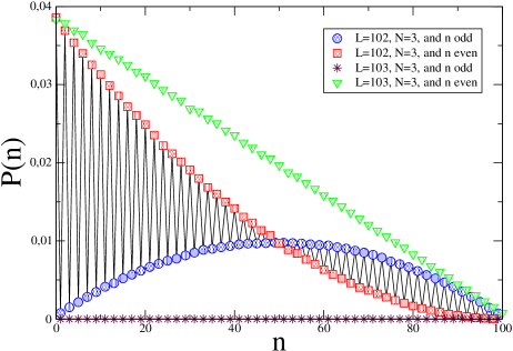
Just the special form of the correction differs for even and odd number of holes. Consider now explicitly a finite number of particles. The weights can be obtained easily from the algebraic rules. For two particles the weights are of the form $f(2l+1,2m)=1+l\beta$. For three particles we find $f(2l+1,2m,2n)=1+(l+n)\beta+\left(\frac{l(l+1)}{2}+ln\right)\beta^{2}$, and so on. From these formulae the probabilities $P(n)$ to find a gap of $n$ sites ($n=0,1,\dots 4$) can easily be calculated. The results are shown in figure 3. One sees the remarkable change of the distribution by adding a single empty site to the system. Note that the probability for an odd gap is of order $1/N$ and thus independent of $L$. Therefore the qualitative form of holds also for $L\rightarrow\infty$.

Figure 3: Headway distribution $P(n)$ for $p_{2}=1$, $p_{1}=0$, and $\beta=1$ for $N=3$ and $4$ and $L=102$ and $103$.

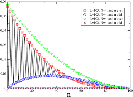
For the thermodynamic limit, one might directly make use of the density profile [2, 16].

It is interesting that the single ‘excess hole’ created by the dynamics leads to effects also in the thermodynamic limit. Although the probability $P(n)$ as predicted by mean field is thermodynamically exact, the system reaches no product-measure steady state, since around the defect a nontrivial density profile is formed. Beyond that a phase transition takes place equivalent to a transition in the defect ASEP [16]. In terms of the different density ($\rho$ in the (defect) ASEP becomes here $2\rho/(1+\rho)$) the critical density is $\rho_{c}=\beta/(2-\beta)$. In the following let us in analogy refer to the $01$-pair as the defect. Since we have $\alpha=1$ the phase diagram of the defect ASEP reduces to a single line.

• For $\rho>\rho_{c}$ the defect behaves as the other particles. In front of the defect the density profile decreases exponentially to its bulk value. The density behind is constant.
  

• For $\rho<\rho_{c}$ the defect is similar to a second-class particle [17] that lowers the average speed of the other particles. The density profile decays algebraically to the bulk value. Behind the defect the density is decreased and the profile increases in the same way to its bulk value as in front. The profile is the limit of a shock profile with equal densities to the left and right.

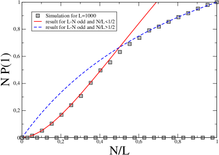
From the relation to the defect ASEP one can obtain the probabilities $P(2n+1)$ for odd headway. For example $P(1)$ is related to the probability $\rho_{-}$ in [16] to find a particle directly behind the defect. Since in our process the defect can be any of the $N$ particles one has

$$[P(1)](\rho)=\cases{\frac{4\rho^{2}}{\beta N(1+\rho)^{2}},&for $\rho<\rho_{c}$,\\ \frac{2\rho}{N(1+\rho)},&for $\rho>\rho_{c}$.}$$ (44)

Figure 4 shows $P(1)$ scaled with $N$ versus the density for $\beta=2/3$, so that the phase transition happens at $\rho_{c}=1/2$. Depicted are the analytic formulae from (44) together with a computer simulation for $L=1000$ with $N$ increased in steps of $\Delta N=25$.

Figure 4: $P(1)$ versus $\rho$ for $\beta=2/3$. See text for details.

3.3 Relation with generalized zero-range processes

In the previous section we expressed the steady state of the system through the set of gaps between particles. This formally corresponds to a mapping onto a model in which a site occupied by particle $\mu$ becomes site $\mu$ and the gap $n_{\mu-1}$ to the left becomes the ‘mass’ on site $\mu$. The ansatz (20) then becomes site-oriented. The corresponding process comprises $N$ sites and $M:=L-N$ particles. In the process obtained from (3) by this mapping one or two particles may leave a certain site with rates:

$$\gamma(l|m)=\cases{1,&for $l=2,m>1$,\\ \beta,&for $l=1,m=1$.}$$ (45)

However this is a special case of the class of generalized zero-range processes introduced by Evans, Majumdar and Zia [10] and referred to as ‘mass-transport models’ (MTM). They derived a necessary and sufficient condition for the steady state to factorize, i.e. $P(m_{1},m_{2},\dots,m_{N})\propto\prod_{\nu=1}^{N}f(m_{\nu})$. The condition on the chipping functions $\gamma$ reads [10, 11]:

$$\gamma(l|m)=\frac{w(l)f(m-l)}{f(m)},{\rm for}\;l=1,\dots,m$$ (46)

where $w(l)$ is an arbitrary non-negative function of $l$. For the process (45) the situation is slightly more special. Here we have a factorized steady state only for even mass and thus it is not predicted by (46). In our rather singular case, involving vanishing single-site weights, (46) is not fulfilled, as is easily seen for $\gamma(1|m)$. To understand this, let us consider a slightly more general case. Assume general single-site weights that vanish for odd masses as it is the case for (45). Considering the master equation shows that the restrictions for the chipping function to recognize the factorized state for $M$ even, are:

$$\gamma(l|m+l)=\cases{{\rm free},&for $m+l$ odd,\\ 0,&for $l,m$ both odd,\\ \frac{x(l)f(m)}{f(m+l)},&for $l,m$ both even.}$$ (47)

However the choice for $f(m)$ in turn implies that the total mass $M=\sum_{i=1}^{L}m_{i}$ is even. Otherwise the normalization

$$Z_{N,M}=\sum\limits_{\{m_{i}\}}\delta\left(M-\sum_{j}m_{j}\right)\prod\limits_{i=1}^{N}f(m_{i})$$ (48)

would vanish. The solution can be used to obtain new solvable models: The process (45) leads to a matrix-product state for the choice of $M$ for which the system can not reach the factorized state. This suggests that the general model (47) with odd particle number (defined trough the weights for even $M$) may also lead to a matrix-product state by special choice of the free parameter in (47). Of course these arguments can be generalized to other choices of vanishing weights [15]. Beyond that, the single-site mass-distribution should equal thermodynamically the result obtained from the case where it is factorizable, since in the infinite system a local perturbation changes the density profile but not the single-site distributions. This way one can obtain the exact distributions also for cases where the steady state has not generally a product measure.
Some focus has recently be attended to two-species zero-range processes and conditions for a factorized steady state [9]. We consider model parameters that violate this condition. Denote the number of first-class particles on site $l$ by $n_{l}$ and the number of second-class particles as $m_{l}$. The rates $u(n,m)$ and $v(m,n)$ at which first and second-class particles move are taken as

$$u(n,m) = 1,\quad\quad\quad\quad\quad{}{\rm for}\;n\geq 1,$$ (49)

$$v(m,n) = \beta\left[1-\theta(n)\right],\quad{\rm for}\;m\geq 1.$$ (50)

The motivation for this choice is simply that the steady state of the MTM (and equivalently (3)) corresponds to the case of a single 2-particle here (pairs of particles in the mass-transport model are mapped onto 1-particles in the ZRP, and the single excess particle is mapped onto the 2-particle). The resulting algebra then also becomes a consequence of (39).

4 Conclusion and outlook

To summarize, a simple traffic model that generalizes the ASEP with periodic boundaries has been considered. In this continuous-time process, particles can move one or two sites to the right. This mimics a larger maximum velocity of cars that is typical for discrete traffic models [3]. Some preliminary results have already been published [20]. We considered choices of hop rates that are not appropriate for modeling traffic but are of theoretical interest. A mean-field theory in comparison with simulations showed that the headway distribution of particles show even/odd oscillations. We considered a special choice of the parameters (see (3)) for which the oscillations become maximal. The matrix-product ansatz was generalized to obtain the exact solution for finite number $N$ of particles and sites $L$. Thermodynamically a crucial phase transition appears: Particles move at their desired maximum velocity $v_{max}$ which leads to the formation of headway being a multiple of $v_{max}$. If there remains smaller headway, then it moves through the system against the direction of motion as a sort of defect. This defect (being somewhere in the system) changes locally the density profile but not the headway distribution of a single particle. Therefore the system is not described by a product measure although the asymptotic headway distribution is given by the mean-field result. Instead the solution is the matrix-product state for the ASEP with a single defect [16]. Note that the process with parallel dynamics leads to a similar stationary state with additional attraction between particles and hole-pairs and can also be solved [5].
We established a relation between non-ergodic exclusion processes with higher velocities, generalized zero-range processes (ZRP) and defect systems. This way one can calculate exact quantities without knowing the exact density profile. For future work it is interesting to investigate the connection between systems with creation and annihilation of ‘defects’ and generalized ZRP to be able to handle ergodic dynamics without parity dependence.
The condition for a simple factorized state in the ASEP considered here is that the rate at which a particle moves a certain number of sites is independent on the headway. This condition holds also for parallel dynamics [22] and higher $v_{max}$. We investigated a slightly more general parameter line, where the rate at which a particle can change its headway does not depend on its length which allows for oscillations in the headway distribution. The mean-field assumption leads to a remarkable agreement with computer simulations. We pointed out the Fibonacci case whose corresponding mass-transport model (on two sites) has a factorized steady state. The single-site weights become Fibonacci numbers $s(n)=F_{n+1}$. The recursion relation (2) becomes $f(m,n)=f(m-1,n)+f(m-2,n)$, for $m\geq 2$, which can be expressed as a matrix-product state $f(m,n)={\rm tr}\;\left(DE^{m}DE^{n}\right)$ with $DEE=DE+D$. However neither the factorization nor the matrix recursion hold for more than two particles. So this case remains unsolved. A comparable good agreement with mean field has been observed previously for the ASEP with shuffled update [24] where also the two-particle state is factorizable. It would be interesting to find out whether the mean-field result in these models is generally exact although the process has not a product measure. Beyond that, the connection between the solvability for two particles and $N$ particles is still an open problem. Here one might be able to profit from knowledge in equilibrium statistical mechanics [25].
We would like to thank A. Schadschneider for helpful discussions.

References

- [1] Chowdhury D, Santen L, and Schadschneider A 2000 Phys. Rep. 329, 199
- [2] Derrida B 1998 Phys. Rep. 301:65
- [3] Nagel K and Schreckenberg M 1992 J. Phys. I France 2 2221- 2229
- [4] Schadschneider A and Schreckenberg M 1997 J. Phys. A 30 L69-L75
- [5] Woelki M and Schreckenberg M 2009 submitted to J. Stat. Mech.
- [6] Krebs K 2000 J. Phys. A: Math. Gen. 33 L149-L154
- [7] Evans M R 1996 Europhys. Lett. 36 13–18
- [8] Evans M R 2000 Braz. J. Phys. 30 42
- [9] Evans M R, Hanney T 2005 J. Phys. A 38 R195
- [10] Evans M R, Majumdar S N and Zia R K P 2004 J. Phys. A 37 L275
- [11] Zia RKP, Evans M R, and Majumdar S N 2004 J. Stat. Mech. L10001
- [12] Evans M R, Rajewsky N and Speer E R 1999 J. Stat. Phys. 95 45–96
- [13] Derrida B, Evans M R, Hakim V and Pasquier V 1993 J. Phys. A 26:1493–1517
- [14] Schreckenberg M, Schadschneider A, Nagel K and Ito N 1995 Phys. Rev. E 51 4 2939–2949
- [15] Woelki M Dissertation Universität Duisburg-Essen not yet published
- [16] Mallick K 1996 J. Phys. A 29:5375–5386
- [17] Derrida B, Janowsky S A, Lebowitz J L and Speer E R 1993 J. Stat. Phys. 73:5/6 813–843
- [18] Liggett T M 1985 Interacting Particle Systems Springer
- [19] Levine E, Ziv G, Gray L and Mukamel D 2004 Physica A 340:636
- [20] Woelki M and Schreckenberg M 2008 in Schreckenberg M Conference Proceedings Traffic and Granular Flow 2007, Springer
- [21] Antal T and G M Schuetz 2000 Phys. Rev. E 62 83 – 93
- [22] Woelki M, Schreckenberg M, and Schadschneider A in preparation
- [23] Klauck K and Schadschneider A 1999 Physica A 271:102
- [24] Woelki M, Schadschneider A and Schreckenberg M 2006 J. Phys. A 39 33–44
- [25] Baxter R 1982 Exactly solved models in statistical mechanics, London: Academic Press Inc.