Dynamical inference from a kinematic snapshot:
The force law in the Solar System

Abstract

If a dynamical system is long-lived and non-resonant (that is, if there is a set of tracers that have evolved independently through many orbital times), and if the system is observed at any non-special time, it is possible to infer the dynamical properties of the system (such as the gravitational force or acceleration law) from a snapshot of the positions and velocities of the tracer population at a single moment in time. In this paper we describe a general inference technique that solves this problem while allowing (1) the unknown distribution function of the tracer population to be simultaneously inferred and marginalized over, and (2) prior information about the gravitational field and distribution function to be taken into account. As an example, we consider the simplest problem of this kind: We infer the force law in the Solar System using only an instantaneous kinematic snapshot (valid at 2009 April 1.0) for the eight major planets. We consider purely radial acceleration laws of the form $a_{r}=-A\,[r/r_{0}]^{-\alpha}$, where $r$ is the distance from the Sun. Using a probabilistic inference technique, we infer $1.989<\alpha<2.052$ (95 percent interval), largely independent of any assumptions about the distribution of energies and eccentricities in the system beyond the assumption that the system is phase-mixed. Generalizations of the methods used here will permit, among other things, inference of Milky Way dynamics from Gaia-like observations.

§ 1 Introduction

The Gaia Satellite (Perryman et al., 2001) will measure positions and velocities for millions to billions of stars at varying precision. One of the principal goals of this mission is to provide the data necessary to infer the dynamical state of the Milky Way. However, there are issues in principle with inference of dynamics from a snapshot or instantaneous set of configuration and velocity measurements: The instantaneous positions and velocities have no necessary relationship with the gravitational potential or accelerations. Indeed, despite a considerable literature (for example, Oort, 1932; Schwarzschild, 1979; Little & Tremaine, 1987; Kaasalainen & Binney, 1994; Johnston et al., 1999; Beloborodov & Levin, 2004) there is no methodology for performing this inference that naturally handles all of the issues, including finite and non-trivial observational uncertainties or noise, missing data, non-steady aspects of the mass distribution, and the (incredibly likely) possibility that the potential is not (simply) integrable. Robust inference may not even be possible if the Milky Way has significant time-dependence or is strongly chaotic or is far from showing any simple symmetries (such as axisymmetry).

Certainly there is no hope for dynamical inference on the massive scale required for the Gaia data set if we cannot perform it on much simpler, much more symmetrical, much older (in a dynamical sense), and much smaller (in a data sense) systems. In what follows, we take one of the simplest possible systems—the Solar System—and the smallest possible data set—the positions and velocities of the major planets at a moment in time—and perform a complete dynamical inference. For a test system we could also have chosen the black hole at the Galactic Center, where similar considerations apply. However, this system has additional issues with “missing data” because not all six phase-space coordinates are directly measurable for all stars. The Solar System truly is the simplest problem in this class.

Our inferential starting point is orbital roulette (Beloborodov & Levin, 2004). In this previous work, it was assumed that the orbital angles (in the action–angle formalism) are uniformly distributed. Thus, dynamical model parameters that correspond to orbital angles that suspiciously lack diversity are rejected. More specifically, the method considers a large range of possible dynamical model parameters, computes orbital angles at every value of the parameters, and a distribution statistic on those orbital angles. If the distribution statistic is designed to monotonically increase with the diversity of the angles or the flatness of the angle distribution, the “best fit” dynamical model parameters are those that optimize the distribution statistic. This kind of approach is inherently frequentist: on many applications of these procedures to independent datasets a confidence interval captures the true dynamical parameters on a guaranteed fraction of trials. However, for any given dataset the confidence interval produced might not represent a credible set of parameters.

In what follows we cast the dynamical parameters estimation as a probabilistic inference problem (a “Bayesian” approach). We adopt the same core assumption as the roulette problem: we assume that the orbital angles are uniformly distributed. However, in this framework, we must also construct prior probability distribution functions for the dynamical model parameters and conditional probabilities of the data given the model to encode the assumptions of a long-lived and bound Solar System. These prior and conditional probability distributions and the data create posterior probability distribution functions for all the parameters. We use this new method to infer the gravitational force law (radial dependence and amplitude). What is new here, in the context of Solar System dynamics, is that we perform this inference with only a snapshot of the kinematic state, that is, with only the positions and velocities of the planets at a single instant of time.

Of course the kinematic snapshot we employ is, in fact, a set of initial conditions for a Solar System integration (Giorgini et al., 1996). These initial conditions were determined not by a single measurement at a single epoch, but are in fact the result of an optimization of a Solar System integration to observed planetary positions over many decades. In the context of this paper—a demonstration of a method—it is best to think of these “data” as “simulated data” useful for testing the method. They just happen to be data that have been simulated by the analog computer we know as the Solar System.

What is new here, in the context of dynamical inference, is that our method is fully probabilistic or Bayesian. This is important for future problems, such as the Gaia problem, or for inferring the mass of the black hole at the center of the Milky Way, because in these real data analysis problems, the data points come with non-trivial and highly correlated observational uncertainties, and because entire dimensions of phase space are missing or unobserved. At the Galactic Center, we do not know the radial distance to anything accurately, and in the Gaia data set many of the radial velocities will not be measured. The Bayesian framework handles these real-world data issues very naturally, although in fact they are not important in the test problem we solve here. Aside from these issues of principle, it is also the case, as we will show, that the Bayesian method performs extremely well.

Of course, a lot is known about the gravitational force law in the Solar System, so we do not expect, at the outset, to be surprised by our results. The first force-law inference in the Solar System (Newton, 1687, and also work by contemporaries, particularly Hooke, who may have priority) made use of full orbit shape determination (Kepler, 1609). In this sense, Newton’s problem—find the force law (from among a small, discrete group of possible force laws) that leads to elliptical orbits with the Sun at one focus—was much easier than the problem we have set for ourselves. Of course, along the way, Newton had to develop for the first time the general principles of kinematics and dynamics!

§ 2 Parameterized force law or dynamical model

We are going to assume spherical symmetry of the Solar System’s force law and gravitational potential, although nothing in the general inference formalism that follows will require this. Consider a radial force law (really acceleration law) of the form

$$\boldsymbol{\vec{a}}=-A\,\left[\frac{r}{r_{0}}\right]^{-\alpha}\,\boldsymbol{\hat{r}}\quad,$$ (1)

where $A$ is an amplitude, $r$ is the distance from the Sun, $r_{0}$ is a distance scale (in this case we will use $r_{0}=1\,\mathrm{AU}$ so that $A$ can be thought of as the acceleration at Earth’s orbit), $\alpha$ parameterizes the radial dependence, and $\boldsymbol{\hat{r}}$ is the radial direction. In this model, the list of free parameters is

$$\boldsymbol{{\omega}}\equiv\{\ln A,\alpha\}\quad,$$ (2)

where we have taken the logarithm of $A$ because in inference problems, dimensioned parameters are usually best handled in the log (Jeffreys, 1939; Sivia & Skilling, 2006).

The potential $u$ (potential energy per unit planet mass), radial effective potential $u_{\mathrm{eff}}$, and binding energy per unit mass $\epsilon\equiv-E/m$ are

$$u(r)=\frac{A\,r_{0}}{1-\alpha}\,\left[\frac{r}{r_{0}}\right]^{1-\alpha}\quad,$$ (3)

$$u_{\mathrm{eff}}(r)=u(r)+\frac{j^{2}}{2\,r^{2}}\quad,$$ (4)

$$\epsilon=-u_{\mathrm{eff}}-\frac{1}{2}\,v_{r}^{2}\quad,$$ (5)

where $j^{2}$ is the square of the magnitude of the planet’s angular momentum per unit mass (or $L^{2}/m^{2}$), and $v_{r}$ is the radial component of the velocity (the component of $\boldsymbol{\vec{v}}$ parallel to $\boldsymbol{\vec{x}}$). The perihelion and aphelion distances $r_{\mathrm{peri}}$ and $r_{\mathrm{ap}}$ are both found by setting $\epsilon=-u_{\mathrm{eff}}$. With these, we can define a radial asymmetry $e$ as

$$e\equiv\frac{r_{\mathrm{ap}}-r_{\mathrm{peri}}}{r_{\mathrm{ap}}+r_{\mathrm{peri}}}\quad,$$ (6)

where we have called this “$e$” because in the Kepler–Newton $\alpha=2$ case it is the orbital eccentricity. One way of thinking of this radial asymmetry is that at any point in the space made up of the dynamical parameters $\boldsymbol{{\omega}}$ and the binding energy $\epsilon$, the radial asymmetry $e$ is a dimensionless description of the angular momentum magnitude.

Importantly for what follows, we can define a “radial angle” $\phi_{r}$ that increases linearly with time from perihelion passage through next perihelion passage. Any planet at radius $r$ on an orbit with perihelion distance $r_{\mathrm{peri}}$ and aphelion distance $r_{\mathrm{ap}}$ can be assigned this angle $\phi_{r}$ by

$$\phi_{r}\equiv\left\{\begin{array}[]{cl}\displaystyle\pi\,\frac{t(r)-t(r_{\mathrm{peri}})}{t(r_{\mathrm{ap}})-t(r_{\mathrm{peri}})}&\mbox{for $v_{r}>0$}\\[10.76385pt] \displaystyle\pi+\pi\,\frac{t(r)-t(r_{\mathrm{ap}})}{t(r_{\mathrm{peri}})-t(r_{\mathrm{ap}})}&\mbox{for $v_{r}<0$}\end{array}\right.\quad,$$ (7)

where the first numerator is the time it takes to go from $r_{\mathrm{peri}}$ to $r$ outbound, the first denominator is the time it takes to go from $r_{\mathrm{peri}}$ to $r_{\mathrm{ap}}$ outbound, the second numerator and denominator are the times inbound, and all time differences between two radii can be computed numerically for general values of $\alpha$ by integrating the inverse of the radial velocity between these radii. The first-order form of this integral has an integrable singularity at the perihelion and aphelion, which can be handled by an appropriate change of variables (e.g., Press et al., 2007). A planet observed at a set of random times spanning many orbits will be observed to have radial angles $\phi_{r}$ drawn from a flat distribution in the range $0<\phi_{r}<2\,\pi$. This radial angle is one of the angles in the action–angle formulation of the system, which is integrable for the simple reason that it is spherically symmetric.

§ 3 Kinematic data

In what follows, we are going to use and compare several methods for inferring the force-law parameters $\boldsymbol{{\omega}}$ (the amplitude $\ln A$ and radial exponent $\alpha$ of the spherical force law) from an instantaneous snapshot of the positions and velocities of the eight major planets. This snapshot was taken from JPL’s HORIZONS System which provides highly accurate ephemerides for Solar System objects (Giorgini et al., 1996). It is an extrapolation (at the time of writing) to 2009 April 1.0, approximately 400 years after the important publication of Kepler (1609). This kinematic snapshot is given in Table 1.

Since this snapshot is obtained by integrating the positions and velocities of Solar System bodies, the accuracy is limited by (i) the correctness of the dynamical model used, (ii) the numerical integration of the equations of motion, and (iii) the accuracy to which the initial conditions are known. It is generally believed that the dynamical model used is correct and complete, and that the numerical integration is sufficiently accurate. The main uncertainty in the ephemerides is then that due to the uncertainty in the initial conditions. The current set of initial conditions (DE405; Standish, 1998) is a fit to a set of optical, radar, and VLBI observations as well as to a set of spacecraft range and Doppler points from various space missions. The uncertainties are the largest for the outer planets, since the data for these are almost entirely from optical observations (with the exception of Jupiter), and because Neptune has not been observed over a full orbit since the start of precise measurements. A comparison between the DE405 ephemerides and more recent observations shows that the positions of the inner planets are known to a fractional accuracy of approximately $10^{-8}$, while those of the outer planets are known to a fractional accuracy of $10^{-6}$ to $10^{-7}$ (Standish, 2004). Uncertainties in the velocities are at the same fractional magnitude.

This kinematic snapshot is not, of course, a fair data set with which to perform the inference below, for the main reason that the “measured” kinematic state of the Solar System is in fact the output of fitting observations with a dynamical model that assumes $\alpha=2$. For this reason, the data should be thought of as “idealized” or “simulated data” and the work must be considered a test of the method rather than a definitive inference.

§ 4 Bound, virialized, and long-lived

The virial theorem relates the time averages $\left<T\right>$ and $\left<U\right>$ of a test particle’s kinetic and potential energies through

$$\left<T\right>=\frac{1-\alpha}{2}\,\left<U\right>\quad,$$ (8)

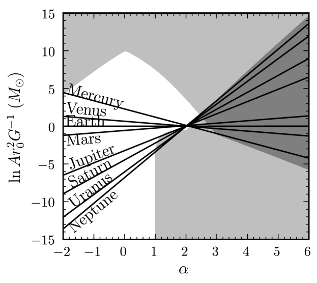
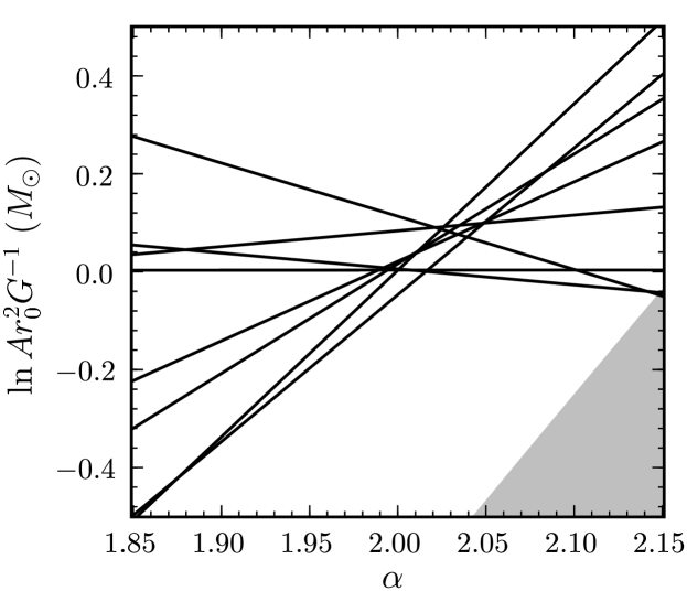
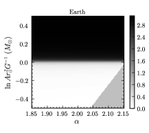
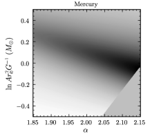
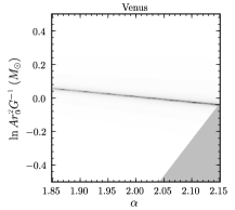
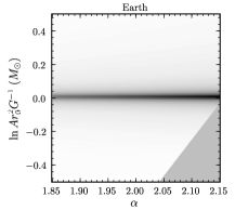
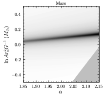
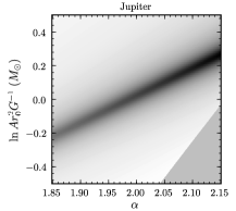
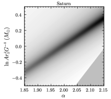
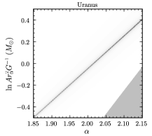
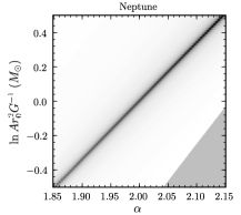
where $\alpha$ is the exponent in the radial force law. Given that a planet’s potential energy is a function of the dynamical parameters $\boldsymbol{{\omega}}$, while its kinetic energy is not, the virial relation for each planet becomes a one-dimensional locus in the $\boldsymbol{{\omega}}$ space. Using kinetic and potential energies computed from the observations as a proxy for the time-averaged energies, these loci are shown in Figures 1 and 2. The fact that all eight lines cross near a single point in the space is encouraging that the system is virialized (as we expect) and that the inference will work. That the eight lines so nearly intersect in a single point is because, in fact, many of the planets are on circular orbits; the probabilistic method developed in this paper does not assume this, but it does retain the precision that is possible because of this situation.

Also shown in Figures 1 and 2 is the region of parameter space in which one or more of the planets is unbound because $T>U$ or, equivalently, $\epsilon<0$. In what follows, we will assign vanishing probability to regions of parameter space in which one or more planets is unbound. However, as we will see, this does not affect any of our conclusions. Also shown in Figure 1 is the region of parameter space in which one or more of the planets has $r_{\mathrm{peri}}<R_{\odot}$, where $R_{\odot}$ is the radius of the Sun. This part of parameter space ought also to be excluded, although in practice this is not necessary for any of what follows.

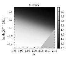
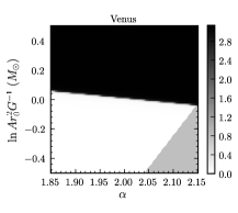
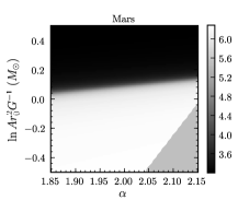
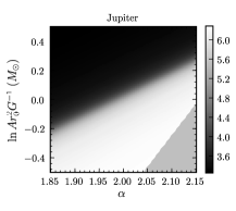
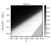
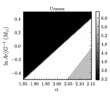
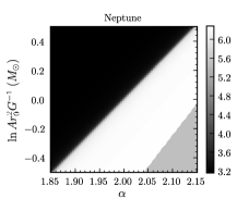
In preparation for what follows, we pre-compute all of the planet radial angles $\phi_{r,i}$—given their positions $\boldsymbol{\vec{x}}_{i}$ and velocities $\boldsymbol{\vec{v}}_{i}$—as a function of the dynamical parameters. These angles are shown in Figure 3.

§ 5 Frequentist orbital roulette

In orbital roulette (Beloborodov & Levin, 2004), the idea is to compute, for each point $\boldsymbol{{\omega}}$ in parameter space, the $N$ radial angles $\phi_{r,i}$ and analyze them statistically for being well mixed. In practice, this means applying a distribution test or multiple distribution tests to the angles and preferring parameters for which these tests are more consistent with a random or flat distribution of angles in the range $0<\phi_{r}<2\,\pi$. Because each test provides one constraint, and in the case described here the parameter space is two-dimensional, at least two qualitatively different tests are required to make localized constraints in $\boldsymbol{{\omega}}$. In addition to a test for a flat angle distribution we also apply a test for an angle–energy correlation.

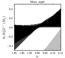
About the simplest consistency test for the calculated angles is a test of the mean of the angles: Is the mean consistent with the expected mean for a uniformly distributed set of $N$ planets? For this to perform well one must fold the angles of the inbound planets onto the interval $[0,\pi]$, that is, disregard the information in the sign of the radial velocity; then the expected mean of the angles is equal to $\pi/2$ (for details on how to test this assumption, see Beloborodov & Levin 2004). The fact that we have to perform this mapping indicates that the procedure is ad hoc. Indeed, for a uniform distribution on the circle there is no specific meaning to the perihelion and the aphelion, or to any two points, such that no real meaning can be attached to the mean of the angles between two arbitrary points on the circle.

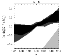
Better, one can test the consistency of the full distribution function of the angles with a uniform distribution. This could again be done with the full $[0,2\pi]$ distributed angles or with the folded angles; the results will depend on this choice. Testing an observed distribution for consistency with an expected distribution often involves comparing cumulative distribution functions (Kolmogorov, 1941). The Kolmogorov–Smirnov (K–S) test is the simplest in practice, since the distribution of the test statistic—the maximum difference between the cumulative distributions—can be approximated by an analytic function (Stephens, 1970). The K–S test is by construction most sensitive to deviations near the median value; this rules out dynamical parameters at which the planets bunch up at perihelion or at aphelion, the situation in which about half are at perihelion and half at aphelion can easily dupe the test.

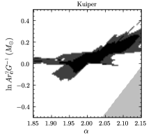
A statistic can be chosen that is sensitive to deviations at all values, such as the Anderson–Darling statistic (Anderson & Darling, 1952). However, no approximate analytic description of the distribution of this statistic exists and in practice this distribution has to be obtained by Monte Carlo sampling (e.g., Beloborodov & Levin, 2004). A statistic more appropriate to the problem at hand (although we are not primarily interested in a careful examination of the differences between different frequentist procedures) is Kuiper’s statistic (Kuiper, 1962). This statistic—the sum of the maximum distance of the observed cumulative distribution above and below the expected cumulative distribution—is invariant under periodic shifts of the angle and was specifically designed to test uniform distributions on the circle. The advantage over Anderson–Darling is that the asymptotic distribution of the Kuiper statistic is known (e.g., Press et al., 2007).

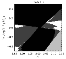
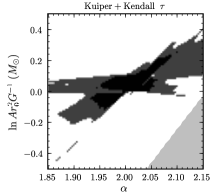
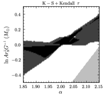
All of these tests for the uniformity of the distribution of the angles are shown in Figure 4. These tests can fail when for a certain combination of dynamical parameters some planets are near aphelion while other planets are near perihelion. This situation appears here in Figure 3, at $\alpha$ far from $2$, where there are large regions in which the inner planets, especially Mercury and Venus, are near perihelion, while the outer planets, especially Uranus and Neptune, are near aphelion and vice versa. This prevents the mean angle and K–S tests from excluding those regions. The Kuiper test performs better.

A second constraint (for the two-dimensional parameter space) comes from a second test. In regions of parameter space in which the inner planets are all near perihelion and the outer planets are all near aphelion, a significant correlation between the angles and the energies exists. This correlation is unphysical if the system is not being observed at any special time. A non-parametric test for the correlation is preferred here as the angle–energy correlation will not in general be linear. We perform a test of the angle–energy correlation using Kendall’s $\tau$ (Kendall, 1938). This is a rank test; it only considers the relative ordering of the angles and energies of different planets (for details on this test see Press et al. 2007). That this test is in a sense orthogonal to the tests of the uniformity of the angle distribution can be seen in Figure 4.

All of the frequentist tests permit acceptance or rejection of a dynamical model at a certain confidence level. 95 and 99 percent confidence intervals for all of the frequentist tests are shown in Figure 4. Also shown is the combination of the tests of the uniformity of the angle distribution with the test of the angle–energy correlation.

§ 6 Probabilistic dynamical inference

The frequentist procedures perform reasonably well in this simple problem because the number of dynamical parameters is small and the data have vanishing errors and no missing components. As the number of dynamical parameters increases the frequentist must find larger numbers of tests in order to break degeneracies. While data uncertainties can be included by sampling the error distribution of the data and combining the results (e.g., Beloborodov & Levin, 2004), this will perform badly in the limit of low signal-to-noise or missing data. These difficulties are related to the fact that these procedures use only a very crude model of the data, that is, that the angles are distributed uniformly and that angle–energy correlations should be absent, which allows no room for discovery of structure in phase space. A fully Bayesian treatment of this problem can treat the phase-space distribution function as an unknown function to be inferred from the data. Modeling the full phase-space distribution function permits simultaneous inference of missing data and properly marginalized probability distributions for dynamical parameters.

Imagine that we have the three-vector positions $\boldsymbol{\vec{x}}_{i}$ and three-vector velocities $\boldsymbol{\vec{v}}_{i}$ at some time $t$ for $N$ planets $i$ and a parameterized model for the gravitational acceleration law (force law per unit mass) $\boldsymbol{\vec{a}}_{\boldsymbol{{\omega}}}(\boldsymbol{\vec{x}})$, a function of position $\boldsymbol{\vec{x}}$ and a list of parameters $\boldsymbol{{\omega}}$. We wish to obtain an estimate of the posterior probability distribution $p(\boldsymbol{{\omega}}|\{\boldsymbol{\vec{x}}_{i},\boldsymbol{\vec{v}}_{i}\})$ for the parameters, where $\{\boldsymbol{\vec{x}}_{i},\boldsymbol{\vec{v}}_{i}\}$ is the set of all planet positions and velocities. We employ Bayes’s theorem as follows:

$$p(\boldsymbol{{\omega}}|\{\boldsymbol{\vec{x}}_{i},\boldsymbol{\vec{v}}_{i}\})=\frac{p(\{\boldsymbol{\vec{x}}_{i},\boldsymbol{\vec{v}}_{i}\}|\boldsymbol{{\omega}})\,p(\boldsymbol{{\omega}})}{p(\{\boldsymbol{\vec{x}}_{i},\boldsymbol{\vec{v}}_{i}\})}\quad,$$ (9)

where, as usual, $p(\{\boldsymbol{\vec{x}}_{i},\boldsymbol{\vec{v}}_{i}\}|\boldsymbol{{\omega}})$ is the likelihood or the probability distribution function for the data given the model parameters, evaluated at the observed values of the data, $p(\boldsymbol{{\omega}})$ is the prior probability distribution function for the parameters, and the denominator is (for our purposes here) a normalization constant.

For our chosen parameterization of the dynamical parameters, $\boldsymbol{{\omega}}$, a broad flat or uniform prior in the space represents a reasonable description of our (assumed) prior knowledge. The much more challenging problem is to specify the likelihood of the dynamical parameters, the conditional probability distribution function $p(\{\boldsymbol{\vec{x}}_{i},\boldsymbol{\vec{v}}_{i}\}|\boldsymbol{{\omega}})$. Without detailed knowledge of how the Solar System formed, this probability distribution is also a representation of our prior beliefs. Ideally our ability to learn from the observed data will not be too sensitive to these beliefs.

It is easier to express beliefs about the angle $\phi_{r}$, radial asymmetry $e$, and binding energy $\epsilon$ of each planet than its position and velocity. This is because, given our assumption that the planets constitute an angle-mixed population, Jeans’s theorem (Jeans, 1915; Binney & Tremaine, 2008) tells us that the distribution function, which is proportional to the probability of observing a planet at a certain locus in phase space, is only a function of the integrals of the motion. We wish to assign zero probability to dynamical parameters that lead to any of the computed binding energies $\epsilon(\boldsymbol{\vec{x}}_{i},\boldsymbol{\vec{v}}_{i},\boldsymbol{{\omega}})$ being negative (because we defined $\epsilon>0$ to be bound). We would also like to express our prior information or assumption that the system is long-lived (in units of the dynamical time), that it is non-resonant, and that we are not seeing the system at any special time, or that the radial angles $\phi_{r}$ will be randomly distributed between $0$ and $2\,\pi$. In the absence of any better information, we will try to be as agnostic as possible about the actions (conserved quantities) of the planets but extremely confident that all radial angles $0<\phi_{r}<2\,\pi$ are equally likely.

In the simple spherical or radial situation under consideration here, in which there are no missing data, we can rewrite the likelihood as a function of the planets’ radial coordinates, as the orientation of the orbit does not depend on the dynamical parameters:

$$p(\boldsymbol{\vec{x}},\boldsymbol{\vec{v}}|\boldsymbol{{\omega}})\propto p(r,v_{r},j^{2}|\boldsymbol{{\omega}})=|J(\ln{\epsilon},e,\phi_{r};r,v_{r},j^{2})|\;p(\ln{\epsilon},e,\phi_{r}|\boldsymbol{{\omega}})\quad.$$ (10)

where, again, we have gone to $\ln{\epsilon}$ because dimensioned parameters are usually best handled in the log, and $J(\ln{\epsilon},e,\phi_{r};r,v_{r},j^{2})$ is the Jacobian matrix of all the partial derivatives of $(\ln{\epsilon},e,\phi_{r})$ with respect to $(r,v_{r},j^{2})$. For spherical potentials, this Jacobian is given by

$$|J(\ln{\epsilon},e,\phi_{r};r,v_{r},j^{2})|=\frac{2\,\pi}{T_{r}}\,\frac{1}{\epsilon}\,\left|\frac{\partial e}{\partial j^{2}}\right|,$$ (11)

where the derivative is evaluated at the current location in phase space and $T_{r}$ is the radial period, which depends on the dynamical parameters and the integrals of the motion. For general $\alpha$ this radial period can be computed numerically (see § 2). The derivative of the radial asymmetry with respect to the specific angular momentum squared can be written in terms of the perihelion and aphelion distance as

$$\frac{\partial e}{\partial j^{2}}=Ar_{0}^{\alpha}\,r_{\mathrm{ap}}\,r_{\mathrm{peri}}\frac{r_{\mathrm{ap}}^{3-\alpha}-r_{\mathrm{peri}}^{3-\alpha}}{(r_{\mathrm{ap}}+r_{\mathrm{peri}})^{2}}\,\left[j^{2}-Ar_{0}^{3}\left(\frac{r_{\mathrm{ap}}}{r_{0}}\right)^{3-\alpha}\right]^{-1}\left[j^{2}-Ar_{0}^{3}\left(\frac{r_{\mathrm{peri}}}{r_{0}}\right)^{3-\alpha}\right]^{-1}\,.$$ (12)

In the special case $\alpha=2$ this Jacobian is

$$|J(\ln{\epsilon},e,\phi_{r};r,v_{r},j^{2})|\propto\epsilon^{3/2}\,e^{-1}\,M_{\odot}^{-3}\,$$ (13)

where we have dropped any terms that do not depend on the mass of the Sun.

As well as assuming that the angles are independently and uniformly distributed, we might further assume that the energy and radial asymmetry of each planet were drawn independently:

$$p(\{\ln{\epsilon}_{i},e_{i},\phi_{r,i}\}|\boldsymbol{{\omega}})=\frac{1}{(2\pi)^{N}}\prod_{i=1}^{N}p(e_{i},\ln{\epsilon}_{i}|\boldsymbol{{\omega}})\quad.$$ (14)

However, a priori we do not know the distribution function from which radial asymmetries and binding energies were drawn. Fixing $p(e_{i},\ln{\epsilon}_{i}|\boldsymbol{{\omega}})$ to a broad distribution would be making a strong assumption: regardless of what the data say we would continue to dogmatically believe that the distribution function was broad, which could result in poor inferences about the model as a whole.

We can assume that the planets’ properties were drawn independently and identically distributed, without making strong assumptions about what that distribution was. This is achieved by introducing auxiliary parameters $\boldsymbol{{\theta}}=\{\boldsymbol{{\theta}}_{e},\boldsymbol{{\theta}}_{\epsilon}\}$ that if known would specify the distribution function. Since we do not know these nuisance parameters, introducing a prior $p(\boldsymbol{{\theta}}|\boldsymbol{{\omega}})$ and marginalizing over them,

$$p(\{\ln{\epsilon}_{i},e_{i},\phi_{r,i}\}|\boldsymbol{{\omega}})=\frac{1}{(2\pi)^{N}}\int\mathrm{d}\boldsymbol{{\theta}}\;\,p(\boldsymbol{{\theta}}|\boldsymbol{{\omega}})\prod_{i=1}^{N}p(e_{i},\ln{\epsilon}_{i}|\boldsymbol{{\theta}},\boldsymbol{{\omega}})\quad,$$ (15)

is then part of the inference task. With all of this in place, we apply equation (9) to get the posterior distribution over the dynamical parameters

$$p(\boldsymbol{{\omega}}|\{\boldsymbol{\vec{x}}_{i},\boldsymbol{\vec{v}}_{i}\})\propto\left[\prod_{i=1}^{N}|J(\ln{\epsilon}_{i},e_{i},\phi_{r,i};r_{i},v_{r,i},j_{i}^{2})|\right]\,\int\mathrm{d}\boldsymbol{{\theta}}\;p(\boldsymbol{{\theta}},\boldsymbol{{\omega}})\,\prod_{i=1}^{N}\,p(e_{i},\ln{\epsilon}_{i}|\boldsymbol{{\theta}},\boldsymbol{{\omega}})\quad,$$ (16)

where each planet’s value of $(\ln{\epsilon}_{i},e_{i},\phi_{r,i})$ is a function of phase-space position $(\boldsymbol{\vec{x}}_{i},\boldsymbol{\vec{v}}_{i})$ and dynamical parameters $\boldsymbol{{\omega}}$, and the Jacobian is evaluated at each planet’s value of $(\ln{\epsilon}_{i},e_{i},\phi_{r,i})$.

For situations in which we have missing data or noisy observations, further unknown quantities will be added to the model and marginalized over. As the model becomes more complicated it is more likely that Markov chain Monte Carlo (e.g., Neal, 1993) or other approximate computational methods will be required.

6.1 Basic method

To keep things as simple as possible, at first we model the distribution function $p(\ln{\epsilon},e|\boldsymbol{{\omega}},\boldsymbol{{\theta}})$ as a product of a top-hat function in $\ln{\epsilon}$ from $\ln{\epsilon}_{a}$ to $\ln{\epsilon}_{b}$ with a top-hat function in $e$ from $e_{a}$ to $e_{b}$. In this context, the phase-space parameter list is

$$\boldsymbol{{\theta}}=\{\ln{\epsilon}_{a},\ln{\epsilon}_{b},e_{a},e_{b}\}\quad.$$ (17)

In what follows, we only consider values $A<\ln\epsilon_{a}<\ln\epsilon_{b}<B$, where $A$ and $B$ provide very distant (uninformative) limits (below, we will take the limit), and $0\leq e_{a}\leq e_{b}\leq 1$. These enforce our assumption or prior information that the system is bound.

For our initial model we also set the prior $p(\boldsymbol{{\theta}},\boldsymbol{{\omega}})$ flat or uniform in all the parameters. Now the marginalization required to compute the posterior (equation 16), an integral over all four of the phase-space distribution parameters in $\boldsymbol{{\theta}}$, can be performed analytically; it leaves

$$\begin{split}p(\boldsymbol{{\omega}}|\{\boldsymbol{\vec{x}}_{i},\boldsymbol{\vec{v}}_{i}\})\propto\,\,&[\ln{\epsilon}_{K}-\ln{\epsilon}_{L}]^{2-N}\left[1-[1-e_{L}]^{2-N}-[e_{M}]^{2-N}+[e_{M}-e_{L}]^{2-N}\right]\\ &\quad\times\prod_{i=1}^{N}|J(\ln{\epsilon},e,\phi_{r};r_{i},v_{r,i},j_{i}^{2})|\quad,\end{split}$$ (18)

where $\ln{\epsilon}_{L}$ is the lowest planetary binding energy at this point $\boldsymbol{{\omega}}$ in dynamical parameter space, $\ln{\epsilon}_{K}$ is the highest, $e_{L}$ is the lowest planetary radial asymmetry at this point $\boldsymbol{{\omega}}$, $e_{M}$ is the highest, and we have taken the limit in which the range of the parameters $(\ln{\epsilon}_{a},\ln{\epsilon}_{b})$ goes to infinity, or $A\rightarrow-\infty$, $B\rightarrow\infty$. This posterior probability distribution for $\boldsymbol{{\omega}}$ represents our posterior beliefs marginalized over all possible values of $\{\ln{\epsilon}_{a},\ln{\epsilon}_{b},e_{a},e_{b}\}$ of the tophat model.

6.2 Alternative methods

The results of any inference depend both on the data and on modeling assumptions. Thus, it is always sensible to question any assumptions and investigate how sensitive the results are to them.

The marginalization in our basic method is tractable at the expense of believability: it seems unlikely that the true distribution function over the planet properties is uniform in the chosen parameterization. If the true distribution function is far from this assumption, the inference performed here could be in trouble because the zero prior probability assigned to all other reasonable forms of the distribution function makes it impossible for the model to learn this. This family of distribution functions also has no special status: a distribution which is uniform in one parameterization will not be uniform in another. Instead of modeling the distribution in $(\ln{\epsilon},e,\phi_{r})$, we could have chosen to model the distribution function in terms of $(\ln{\epsilon},e^{2},\phi_{r})$. This set of parameters is, in a sense, more natural as it is closer to action–angle coordinates, and, thus, the Jacobian $|J(\ln{\epsilon},e^{2},\phi_{r};r,v_{r},j^{2})|$ is more close to constant. Indeed, from equation (13) it is clear that, in the case of $\alpha=2$, this Jacobian does not depend on the eccentricity of the orbit any longer and Figure 8 shows that this Jacobian is close to constant for all values of $\ln A$ and $\alpha$. However, it is not obvious a priori whether using this parameterization will give better results. Rather than guessing, we can assume that the distribution over radial asymmetries is uniform in an unknown parameterization, and infer from the data what this parameterization should be. We tried assuming that the radial asymmetry was uniform over some range of $e$, $e^{2}$ or $\sqrt{e}$, with equal prior probability over each choice. This method corresponds to extending $\boldsymbol{{\theta}}$ to parameterize a richer class of distributions. As we did with nuisance parameters before, we can marginalize over this choice.

In general we could marginalize over a very flexible class of distributions for both the binding energy and radial asymmetry. A generic way of representing distributions is with a histogram, where any distribution can be represented within an arbitrary tolerance for sufficiently narrow bins. Some care is required in putting a prior $p(\boldsymbol{{\theta}})$ over the heights of the bins. It is tempting to use a Dirichlet distribution, which allows analytical marginalization. However, this assumes that the heights of the bins are unrelated except through their overall normalization. An arbitrarily spiky distribution function is not only unphysical, but we would be unable to infer its shape from point observations.

We attempted to construct a sensible prior over distributions using histograms with many bins by coupling the heights of the bins so that the densities appear smooth. Since the focus on this paper is on the principles of dynamical inference and not on the specific result on the Solar System’s force law, we only provide a brief description of how we implemented this approach. We refer the interested reader to the references provided in the following for more details on the specifics. A multivariate Gaussian prior can be put over the log bin heights, approximating a logistic Gaussian process (Leonard, 1978). We used 100 equal-width bins coupled with a Gaussian covariance function (Rasmussen and Williams, 2006). We put uniform priors over the start and end points of the histogram and over physically reasonable ranges of the covariance function’s parameters. The posterior over the dynamical parameters was estimated by Markov chain Monte Carlo simulation of all the unknowns, Gibbs sampling was used to update the dynamical parameters over a grid of values for which we had precomputed the Jacobian term. Slice sampling (Neal, 2003) was used to update all nuisance parameters, except the bin heights which were updated with a Metropolis–Hastings method (Neal, 1999, Eq. 15).

§ 7 Results and discussion

In our basic method we evaluate the Jacobian $|J(\ln\epsilon,e,\phi_{r};r_{i},v_{r,i},j_{i}^{2})|$ for each planet at the observed radius, radial velocity, and specific angular momentum, for each value of the dynamical parameters $\boldsymbol{{\omega}}$, and multiply the magnitudes of the determinants of these Jacobians together. Following equation (18) we multiply this product with the value of the marginalized product of the distribution function and finally multiply this with the (uniform) prior on the dynamical parameters in order to obtain the posterior probability distribution for the dynamical parameters.

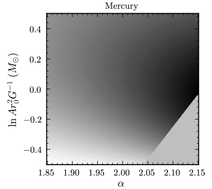
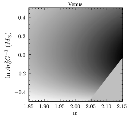
It is instructive to look at the magnitude of the determinant of the Jacobian for each planet as a function of the dynamical parameters in Figure 5. These factors seem to show a clear preference for the dynamical parameters of each planet to lie on its virial locus. Why is this? For nearly circular orbits the last two factors in equation (12) are equal and are unbounded for perfectly circular orbits; this results in a natural preference for nearly circular orbits for all of the planets, i.e., for each planet to lie somewhere along its virial locus. At the same time the measured non-zero radial velocity limits the extent to which a planet’s orbit can be circularized by a suitable choice of the dynamical parameters and, thus, how close to the circular singularity an individual planet can be brought. This naturally leads to a weighting scheme in which planets that are closer to circular orbits (as measured by the observed angle between the planet’s velocity and the tangent to the circular orbit going through its present location) receive a higher weight in the analysis than planets on less circular orbits. This weighting scheme is good in that planets on more circular orbits are indeed more informative about the potential than planets on less circular orbits. Therefore, it may seem that the decision to model the radial asymmetries as uniform in $e$ was fortuitous, but in fact, as we will discuss below in § 7.1, the results obtained using the basic method are robust in that more flexible models learn that the tophat in $e$ leads to a good interpretation of the data.

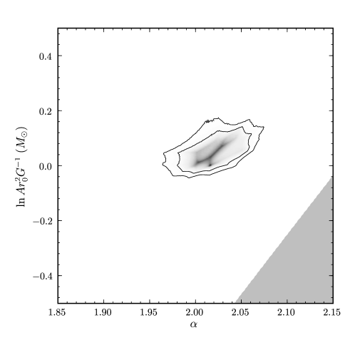
The posterior probability distribution is shown in Figure 6. A strong peak is apparent near $\alpha=2$ and the Newtonian Solar value for $\ln A$. The width of the probability distribution is indicated by the 95 and 99 percent posterior contours. These contours are defined to enclose the smallest area that holds 95 and 99 percent, respectively, of the posterior probability distribution.

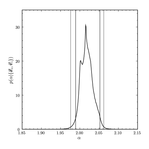
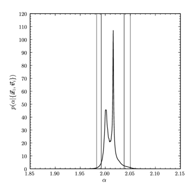
In order to infer the exponent $\alpha$ of the force power-law we perform a second marginalization of the posterior probability distribution, this time over the (for our purposes) uninteresting parameter $\ln A$. This gives a posterior probability distribution for the parameter $\alpha$

$$p(\alpha|\{\boldsymbol{\vec{x}}_{i},\boldsymbol{\vec{v}}_{i}\})=\int\mathrm{d}\ln A\,p(\boldsymbol{{\omega}}|\{\boldsymbol{\vec{x}}_{i},\boldsymbol{\vec{v}}_{i}\})\quad.$$ (19)

This probability distribution is shown in Figure 7. The 95 and 99 percent posterior intervals in this figure are defined to exclude 2.5 and 0.5 percent, respectively, of the distribution on either side of the central region.

The result of the inference is not a value for the parameters but a posterior probability distribution. A “best fit” value for $\alpha$ could be obtained according to various criteria. For example, the posterior mean minimizes the expected square difference from the true parameter. However, since the posterior distribution is multi-modal, a point-estimate does not capture our uncertainty. The posterior is better summarized by a credible interval, containing a given fraction of the probability mass. The 95 percent posterior interval is $1.989<\alpha<2.052$. This compares favorably with the results obtained by Newton (1687) who inferred $\alpha=2$ from a much richer data set (though a less rich model set). Modern tests constrain the value of the exponent $\alpha$ to a fractional accuracy of 10^-8–10^-9 on Solar System scales (Adelberger, Heckel, & Nelson, 2003; Fischbach & Talmadge, 1999) using Lunar Laser Ranging tests (Williams, Turyshev, & Boggs, 2004) and Keplerian tests comparing $G(r)M_{\odot}$ and the rate of precession for different planets (Talmadge et al., 1988).

Our method appears to work well: the true dynamical parameters $A$ and $\alpha$ are plausible under a fairly tight posterior distribution, see Figure 6. The confidence intervals from the frequentist tests, Figure 4, are somewhat broader than the posterior intervals, but are not directly comparable. Frequentist confidence intervals do not represent beliefs about the parameters for this dataset, simply a region that satisfies some sampling properties. As a result it is unsurprising that the frequentist confidence intervals appear less good if interpreted as beliefs given the data. It is difficult to use the frequentist confidence intervals to make statements about $\alpha$ alone: without the assumptions of the Bayesian method we cannot marginalize over the parameter $A$. One approach that allows frequentist guarantees is to set $A$ adversarially, but this pessimistic view would give unreasonably large error bars for $\alpha$.

That the posterior distribution $p(\alpha|\{\boldsymbol{\vec{x}}_{i},\boldsymbol{\vec{v}}_{i}\})$ turns out to be multi-modal is no surprise in the light of the virial considerations from Figures 1 and 2. The two peaks in $p(\alpha|\{\boldsymbol{\vec{x}}_{i},\boldsymbol{\vec{v}}_{i}\})$ correspond to the two main regions in parameter space in which the different virial loci cross. These virial considerations, and also the frequentist techniques, are very similar to the probabilistic approach in that they all prefer each planet to be in a non-special region of radial angle space, that is, between perihelion and aphelion; this can only happen simultaneously near the points in parameter space at which virial loci cross. The advantage of the probabilistic approach is that it explains and quantifies this reasoning, and uses it to set formal limits on the dynamical parameters.

7.1 Sensitivity analysis

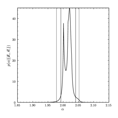
The strongly peaked Jacobian factors shown in Figure 5 depend strongly on the choice of parameterization. If the model was expressed using the radial asymmetries squared rather than the radial asymmetries, the Jacobians, some of which are shown in Figure 8, are much flatter. If the model is maintained by also transforming the prior over radial asymmetry distributions to the new parameterization, the posterior distribution over dynamical parameters will be unchanged. Setting all the radial asymmetries close to one is penalized elsewhere in the mathematical expression.

However, setting the prior over radial asymmetry distributions to consider only uniform distributions was a strong assumption. If we had only considered distributions uniform in the radial asymmetry squared, this combined with the flat Jacobians in Figure 8 would not have given as tight a posterior distribution. Fortunately we can infer a suitable parameterization, or equivalently the distribution function from a richer family of possibilities, from the data.

Figure 9 shows the posterior over $\alpha$ from using the two more flexible priors outlined in § 6.2. Assuming that the radial asymmetry is uniform in one of $\sqrt{e}$, $e$, or $e^{2}$ gave a 95% credible interval of $1.990<\alpha<2.035$. A variety of different flexible priors for the radial asymmetry distribution gave very similar results. Allowing the $\ln A$ constant in the force law to come from a flexible family of distributions changed the posterior very little. The 95% credible interval from the flexible non-parametric prior on both distributions gave a 95% credible interval of $1.991<\alpha<2.040$. The fine details of the posterior distribution, specifically the relative mass in the two modes, are sensitive to prior assumptions. This is unsurprising with only eight data points. However, the position of the bulk of the posterior mass, which gives the confidence interval is surprisingly robust across a wide range of modeling choices.

As a warning, it is possible to obtain poor results through bad modeling choices. The reasonable posterior from our basic method, Figure 7, was to some extent due to chance. The family of possible radial asymmetry distributions is inflexible as it forces this distribution to be flat over some range in radial asymmetry. Using the basic method it is not possible to learn the true distribution, which is not flat in radial asymmetry, from data, because the truth is assigned zero prior probability. We were fortunate to choose a parameterization in which the inflexible family was not too unreasonable. The non-parametric approach is much more flexible in that its weak smoothness constraints assign non-zero prior probabilities to all reasonable distribution functions such that the true one could be picked out with enough data. However, care must also be taken with non-parametric modeling. An unsmooth Dirichlet prior over bin heights in a non-parametric prior over distributions gave a broad and biased distribution over $\alpha$.

7.2 Future work

The necessity of a proper probabilistic approach as laid out in this paper has been recognized before in the context of inferring the mass of the Galaxy from a small set of highly informative tracers: distant satellite galaxies (Little & Tremaine, 1987) and high velocity stars (Leonard & Tremaine, 1990). The limitations of those works are that they choose restrictive forms of the distribution function in which the distribution of angular momentum is fixed as either radial or isotropic, or given as an inflexible parametric function in between these two extrema (Kochanek, 1996). The precision of their results for the fundamental parameters of the Galaxy is limited by the systematic uncertainty arising from this assumption. In the case of estimating the local escape velocity from a sample of high velocity stars, a power law model for the energy part of the distribution function was used; some progress has been made marginalizing over the exponent, a nuisance parameter, with a prior coming from cosmological simulations (Smith et al., 2007). In the future, using the technique introduced in this paper there is no need to make strong assumptions about the degree of anisotropy of the system at hand or the form of the distribution function beyond the assumption of complete angle mixing. The results of this paper show that by introducing flexible models for the distribution function that can learn from the data, robust constraints on the parameters of a dynamical system can be obtained.

The approach developed here can be applied to other (perhaps more pressing) dynamical inference problems in which test particles can be relied upon to be well-mixed in angle space. One such problem is the dynamics in the region surrounding the black hole at the Galactic Center. Often in these problems complications arise because of large observational uncertainties (often highly correlated), the absence of some of the six-dimensional phase-space coordinates, and selection effects, all of which are absent in the simple problem considered here. It will be necessary for these problems to model the full six-dimensional phase-space distribution function. This will complicate the marginalization over the phase-space parameters, which was trivial here in the basic method, but at the same time it will permit the discovery of structure in the phase-space distribution, which can aid with the presence of missing data and large observational uncertainties. That this approach has much potential has been shown before in the case of the Galactic Center; the assumption that a set of stars at the Galactic Center is part of a disk-like population has been successful in reconstructing missing data (Beloborodov et al., 2006). Extension of the approach developed in this paper will permit incorporation of much more of the available data on the dynamics in the central region of the Galaxy. This, in turn, will lead to a better determination of the mass of the black hole and the surrounding density profile.

On larger scales, approaches like that developed in this paper will prove to be essential for the analysis of the large data sets of upcoming surveys such as Gaia. As the duration of the Gaia mission is vanishingly smaller than any dynamical timescale, the problem posed is essentially the same as the problem posed here: Infer the dynamics from a snapshot of the kinematics. Our approach cannot simply be applied to this larger problem because the system is almost certainly not (trivially) integrable, and the assumption of mixed angles and lack of resonances is invalidated by the clear abundance of substructure in the halo (e.g., Willman et al., 2005; Belokurov et al., 2006, 2007; Koposov et al., 2008) and the disk (Dehnen, 1998; Bovy, Hogg, & Roweis, 2009); indeed, Jeans himself, in the paper in which he first wrote down his eponymous theorem (Jeans, 1915), argued against assuming a steady state for the Galaxy. Modeling the details of the phase-space distribution function will be even more important in this context. However, we expect that a large fraction of the Galaxy, even a large fraction of the stellar halo, is well-mixed, such that mixed-angle approaches are expected to lead to valuable inferences. Combining the mixed-angle and unmixed-substructure techniques into a general inference about the dynamics of the Galaxy requires a fully probabilistic method and the approach developed in this paper is a baby step toward this ambitious goal.

Table 1: Planet Ephemerides for 2009-Apr-01 00:00:00.0000 (CT)

Planet	$x$		$y$		$z$		$v_{x}$		$v_{y}$		$v_{z}$
	($\mathrm{AU}$)		($\mathrm{AU}$)		($\mathrm{AU}$)		($\mathrm{AU}$ $\mathrm{yr}^{-1}$)		($\mathrm{AU}$ $\mathrm{yr}^{-1}$)		($\mathrm{AU}$ $\mathrm{yr}^{-1}$)
Mercury	0.	324190175	0.	090955208	-0.	022920510	-4.	627851589	10.	390063716	1.	273504997
Venus	-0.	701534590	-0.	168809218	0.	037947785	1.	725066954	-7.	205747212	-0.	198268558
Earth	-0.	982564148	-0.	191145980	-0.	000014724	1.	126784520	-6.	187988860	0.	000330572
Mars	1.	104185888	-0.	826097003	-0.	044595990	3.	260215854	4.	524583075	0.	014760239
Jupiter	3.	266443877	-3.	888055863	-0.	057015321	2.	076140727	1.	904040630	-0.	054374153
Saturn	-9.	218802228	1.	788299816	0.	335737817	-0.	496457364	-2.	005021061	0.	054667082
Uranus	19.	930781147	-2.	555241579	-0.	267710968	0.	172224285	1.	357933443	0.	002836325
Neptune	24.	323085642	-17.	606227355	-0.	197974999	0.	664855006	0.	935497207	-0.	034716967

Note. — The $xyz$-coordinate system is defined as follows: the $xy$-plane is given by the plane of the Earth’s orbit at J2000.0, the $x$-axis is out along the ascending node of the instantaneous plane of the Earth’s orbit and the Earth’s mean equator at J2000.0, and the $z$-axis is perpendicular to the $xy$-plane in the directional (+ or -) sense of Earth’s north pole at J2000.0. The origin of the coordinate system is given by the barycenter of the Solar System. One year is defined as 365.25 days.

Figure 1: The Virial relation between the kinetic energy and the potential energy (equation [8]) for each of the eight planets in the Solar System. For the combinations of dynamical parameters in the light gray region in the lower right at least one planet becomes unbound. When the dynamical parameters are in the light gray region in the upper left at least one planet has $r_{\mathrm{peri}}<R_{\odot}$. The light gray regions overlap in the dark gray region. In the units used in this Figure, the “true” value of $A$ lies at $\ln Ar_{0}^{2}G^{-1}=0$.

Figure 2: Zoomed in version of Figure 1.

Figure 3: Computed radial angles $\phi_{r}$ for each of the eight planets as a function of the dynamical parameters. The gray triangular region in the bottom-right corner is the region excluded by the condition that all the planets are bound. Each planet has an angle range of $0<\phi_{r}<\pi$ if it has radial velocity $v_{r}>0$ (outgoing from perihelion) or $\pi<\phi_{r}<2\,\pi$ if it has $v_{r}<0$ (incoming from aphelion).

Figure 4: Various frequentist tests applied to test the uniformity of the angle distribution and the absence of angle–energy correlations. From top to bottom, left to right: test of the mean of the angles; K–S test for the uniformity of the angle distribution; Kuiper test for the uniformity of the angles; Kendall $\tau$ test for the absence of angle–energy correlations; combined confidence intervals from the Kuiper test and the Kendall test; combined confidence intervals from the K–S test and the Kendall test. In the plots with a single statistic the darkest region corresponds to the 95 percent confidence region, the lighter region to the 99 percent confidence region. The same is true for the plots with combinations of statistics, except that a Bonferroni correction has been applied to the significances of the individual statistics that make up the combination. In each plot the lightest region is excluded because at least one planet becomes unbound for those parameter values.

Figure 5: Density plots of the absolute value of the determinant $|J(\ln{\epsilon},e,\phi_{r};r,v_{r},j^{2})|$ of the Jacobian of the transformation from the energy $\epsilon$, radial asymmetry $e$, and radial angle $\phi_{r}$ coordinates to the relevant positional and kinematical observables, evaluated at the observed positions and velocities of the planets, as a function of the dynamical parameters. Gray scales are linear with darker shades for larger values.

Figure 6: The posterior probability distribution $p(\boldsymbol{{\omega}}|\{\boldsymbol{\vec{x}}_{i},\boldsymbol{\vec{v}}_{i}\})$ for the dynamical parameters on a linear scale. Contours are 95 and 99 percent posterior regions.

Figure 7: Marginalized posterior probability distribution for the parameter $\alpha$ with 95 and 99 percent posterior intervals.

Figure 8: Density plots of the absolute value of the determinant $|J(\ln{\epsilon},e^{2},\phi_{r};r,v_{r},j^{2})|$ of the Jacobian of the transformation from the energy $\epsilon$, radial asymmetry squared $e^{2}$, and radial angle $\phi_{r}$ coordinates to the relevant positional and kinematical observables, evaluated at the observed positions and velocities of the planets, as a function of the dynamical parameters. Grayscales are linear with darker shades for larger values. Only the Jacobians for Mercury and Venus are shown here; the corresponding Jacobians for the other planets are very similar to these.

Figure 9: Alternative posterior probability distributions for the parameter $\alpha$ with 95 and 99 percent posterior intervals. Top: distribution over radial asymmetry is assumed to be uniform in one of $\sqrt{e}$, $e$ or $e^{2}$. Bottom: results from a non-parametric prior over the distributions of both $e$ and $\ln A$.

References

- Adelberger, Heckel, & Nelson (2003) Adelberger, E. G., Heckel, B. R., & Nelson, A. E., 2003, Annu. Rev. Nucl. Part. Sci., 53, 77
- Anderson & Darling (1952) Anderson, T. W. & Darling, D. A., 1952, Ann. Math. Stat., 23, 193
- Beloborodov & Levin (2004) Beloborodov, A. M. & Levin, Y., 2004, ApJ, 613, 224
- Beloborodov et al. (2006) Beloborodov, A. M, Levin, Y., Eisenhauer, F., Genzel, R., Paumard, T., Gillessen, S., & Ott, T., 2004, ApJ, 648, 405
- Belokurov et al. (2006) Belokurov, V., et al., 2006, ApJ, 642, L137
- Belokurov et al. (2007) Belokurov, V., et al., 2007, ApJ, 654, 897
- Binney & Tremaine (2008) Binney, J. & Tremaine, S., 2008, Galactic Dynamics: Second Edition (Princeton University Press)
- Bovy, Hogg, & Roweis (2009) Bovy, J., Hogg, D. W., & Roweis, S. T., 2009, ApJ, 700, 1794
- Dehnen (1998) Dehnen, W., 1998, AJ, 115, 2384
- Fischbach & Talmadge (1999) Fischbach, E. & Talmadge, C. L., 1999 The Search for Non-Newtonian Gravity, (Berlin: Springer)
- Giorgini et al. (1996) Giorgini, J. D., Yeomans, D. K., Chamberlin, A. B., Chodas, P. W., Jacobson, R. A., Keesey, M. S., Lieske, J. H., Ostro, S. J., Standish, E. M., & Wimberly, R. N., 1996, BAAS, 28, 1158
- Jeans (1915) Jeans, J. H., 1915, MNRAS, 76, 70
- Jeffreys (1939) Jeffreys, H., 1939, Theory of Probability (Oxford: Clarendon Press)
- Johnston et al. (1999) Johnston, K. V., Zhao, H., Spergel, D. N., & Hernquist, L., 1999, ApJ, 512, L109
- Kaasalainen & Binney (1994) Kaasalainen, M. & Binney, J., 1994, Phys. Rev. Lett., 73, 2377
- Kendall (1938) Kendall, M., 1938, Biometrika, 30, 81
- Kepler (1609) Kepler, J., 1609, Astronomia Nova, trans. W. H. Donahue, 1992 (Cambridge University Press)
- Kochanek (1996) Kochanek, C. S., 1996, ApJ, 457, 228
- Kolmogorov (1941) Kolmogorov, A. N., 1941, Ann. Math. Stat., 12, 461
- Koposov et al. (2008) Koposov, S., et al., 2008, ApJ, 686, 279
- Kuiper (1962) Kuiper, N. H., 1962, Proc. Koninklijke Nederlandse Akademie van Wetenschappen A, 63, 38
- Leonard (1978) Leonard., T., 1978, J. Roy. Stat. Soc. B, 40, 113
- Leonard & Tremaine (1990) Leonard, P. J. T. & Tremaine, S., 1990, ApJ, 353, 486
- Little & Tremaine (1987) Little, B. & Tremaine, S., 1987, ApJ, 320, 493
- Neal (1993) Neal., R. M., 1993, Probabilistic Inference Using Markov Chain Monte Carlo Methods. Technical Report CRG-TR-93-1, Department of Computer Science, University of Toronto
- Neal (1999) Neal., R. M., 1999, in Bayesian Statistics 6, ed. J. M. Bernardo et al.. (Oxford University Press), 475
- Neal (2003) Neal., R. M., 2003, Ann. Stat., 31, 705
- Newton (1687) Newton, I., 1687, Philosophiae Naturalis Principia Mathematica, trans. F. Cajori, 1934 (University of California Press)
- Oort (1932) Oort, J. H., 1932, Bull. Astron. Inst. Netherlands, 6, 249
- Perryman et al. (2001) Perryman, M. A. C., et al., 2001, A&A, 369, 339
- Press et al. (2007) Press, W. H., Teukolsky, S. A, Vetterling, W. T., & Flannery, B. P., 2007, Numerical Recipes: The Art of Scientific Computing, 3rd Edition (Cambridge University Press)
- Rasmussen and Williams (2006) Rasmussen, C. E. & Williams., C. K. I., 2006 Gaussian Processes for Machine Learning (MIT Press)
- Schwarzschild (1979) Schwarzschild, M., 1979 ApJ, 232, 236
- Sivia & Skilling (2006) Sivia, D. S. & Skilling, J., 2006, Data Analysis: A Bayesian Tutorial (Oxford University Press)
- Smith et al. (2007) Smith, M. C., et al., 2007, MNRAS, 379, 755
- Standish (1998) Standish, E. M., 1998, JPL Planetary and Lunar Ephemerides, DE405/LE405, JPL IOM 312, F-98-048 (Pasadena, CA: JPL)
- Standish (2004) Standish, E. M., 2004, A&A, 417, 1165
- Stephens (1970) Stephens, M. A., 1970, J. R. Stat. Soc. B, 32, 115
- Talmadge et al. (1988) Talmadge, C., Berthias, J.-P., Hellings, R. W., & Standish, E. M., 1988, Phys. Rev. Lett., 61, 1159
- Williams, Turyshev, & Boggs (2004) Williams, J. G., Turyshev, S. G., & Boggs, D. H., 2004, Phys. Rev. Lett., 93, 261101
- Willman et al. (2005) Willman, B., et al., 2005, ApJ, 626, L85