A Mixture-Based Approach to Regional Adaptation for MCMC

Abstract

Recent advances in adaptive Markov chain Monte Carlo (AMCMC) include the need for regional adaptation in situations when the optimal transition kernel is different across different regions of the sample space. Motivated by these findings, we propose a mixture-based approach to determine the partition needed for regional AMCMC. The mixture model is fitted using an online EM algorithm (see Andrieu and Moulines, 2006; Cappé and Moulines, 2009) which allows us to bypass simultaneously the heavy computational load and to implement the regional adaptive algorithm with online recursion (RAPTOR). The method is tried on simulated as well as real data examples.

Keywords: Adaptive MCMC, regional adaptation, online EM, mixture model.

1 Introduction

In recent years, the Markov chain Monte Carlo (MCMC) class of computational algorithms has been enriched with adaptive MCMC (AMCMC). Spurred by the seminal paper of Haario et al. (2001) an increasing body of literature has been devoted to the study of AMCMC. It has long been known that the fine tuning of the proposal distribution’s parameters in a Metropolis sampler is central to the performance of the algorithm. Haario et al. (2001), Haario et al. (2005), Andrieu and Robert (2001), Andrieu and Moulines (2006), Andrieu et al. (2005) and Roberts and Rosenthal (2007) have provided the theory needed to prove that it is possible to adapt the parameters of the proposal distribution ”on the fly”, i.e. while running the Markov chain and using for tuning the very samples produced by the chain. The AMCMC algorithms may be vulnerable to the multimodality of the target distribution and more care needs to be taken in implementing the AMCMC paradigm. In Craiu et al. (2008) a few possible approaches are discussed, central among which is the regional adaptive algorithm (RAPT) designed for Metropolis samplers. However, the premise for RAPT is that a partition of the sample space is given and it is approximately correctly specified. While sophisticated methods exist to detect the modes of a multimodal distribution (see Sminchisescu and Triggs, 2001, 2002; Neal, 2001) it is not obvious how to use such techniques for defining the desired partition of the sample space. We follow here the methods of Andrieu and Moulines (2006) and Cappé and Moulines (2009) to propose a mixture-based approach for adaptively determining the boundary between high probability regions. We approximate the target distribution using a mixture of Gaussians whose parameters are used to define the partition. The theoretical challenges lie in the fact that the volume of data used for fitting the mixture increases as the simulation progresses and the data is not independent since it is made of realizations of a Markov chain. Both challenges have been tackled by Andrieu and Moulines (2006) and Cappé and Moulines (2009).

In the next section we briefly review the RAPT algorithm and the online EM algorithm of Cappé and Moulines (2009). In section 3 we describe the methodology behind the regional adaptive algorithm with online recursion (RAPTOR). The simulation studies and real data application are discussed in Sections 4 and 5, respectively.

2 Regional Adaptation and Online EM

2.1 Regional Adaptation (RAPT)

Regional adaptation is motivated by the fundamental and natural idea that, in many situations, the optimal proposal distribution used in a Metropolis sampling algorithm may be different in separate regions of the sample space ${\cal{S}}$. For now, assume that we are given a partition of the space ${\cal{S}}$ made of two regions $\mbox{${\cal{S}}$}_{1},\mbox{${\cal{S}}$}_{2}$. The mixed RAPT algorithm for a random walk Metropolis (RWM) sampler uses the following mixture as a proposal distribution

$$Q(x,dy)=(1-\beta)\sum_{i=1}^{2}1_{\mbox{${\cal{S}}$}_{i}}(x)[\lambda_{1}^{(i)}Q_{1}(x,dy)+\lambda_{2}^{(i)}Q_{2}(x,dy)]+\beta Q_{whole}(x,dy),$$ (1)

where $Q_{i}$ is adapted using samples from $\mbox{${\cal{S}}$}_{i}$ and $Q_{whole}$ is adapted using all the samples in ${\cal{S}}$. The mixing parameters $\lambda_{1}^{(i)}$, $i=1,2$ are also adapted while the parameter $\beta$ is constant throughout the simulation. Details regarding the adaptation procedures for the above distributions and parameters can be found in Craiu et al. (2008) who also provide a proof regarding the asymptotic convergence of the algorithm.

One can see that, regardless of the region the chain is currently in, the proposal distribution is a mixture of three distributions: $Q_{1},Q_{2}$ which are approximately optimal choices for the target restricted to $\mbox{${\cal{S}}$}_{1}$ and $\mbox{${\cal{S}}$}_{2}$, respectively, and $Q_{whole}$, which has the purpose of ensuring good traffic between the two regions. The reason we use a mixture with these three components (as opposed to using a mixture with the components $Q_{i}$ and $Q_{whole}$ when the chain is in $\mbox{${\cal{S}}$}_{i}$) is intuitively motivated by the uncertainty of determining the ideal partition $\mbox{${\cal{S}}$}=\mbox{${\cal{S}}$}_{1}\cup\mbox{${\cal{S}}$}_{2}$. The degree of success for RAPT depends on whether the partition used is a relatively good approximation of the ideal one. In the next section we propose to adaptively modify the partition between the two regions using the online EM algorithm.

2.2 Online EM

Denote $\pi$ the target distribution of interest. Working under the assumption that $\pi$ is multi-modal one can try to approximate $\pi$ using a mixture of Gaussian distributions. The approximation is in many cases accurate once the distribution $\pi$ can be well approximated by a Gaussian in a neighborhood of each local mode. The analysis of mixture models has relied for a while now on the EM algorithm (Dempster et al., 1977) as discussed by Titterington et al. (1985) and references therein. In the MCMC setup the amount of data available to fit the mixture increases as the simulation progresses, therefore making unfeasible the traditional implementation of the algorithm. An added complication is that the streams of data contain dependent realizations as they are produced by running one or more Markov chains. Both difficulties are dealt with effectively by Andrieu and Moulines (2006) who propose an online EM algorithm that updates the parameter estimates as more data become available. The algorithm is further refined by Cappé and Moulines (2009).

The M-step for the classical EM algorithm involves the maximization (in $\theta$) of

$$Q_{\theta^{\prime}}(y_{1:n};\theta)=\sum_{i=1}^{n}E[\log f(X_{i};\theta)|\theta^{\prime},y_{i}]$$

where $Y_{1:n}$ are the $n$-dimensional observed data and $X_{i}$ is the $i$-th unit complete data.

The online EM of Andrieu and Moulines (2006) modify the $Q$ function to

$$\hat{Q}_{n+1}(\theta)=\hat{Q}_{n}(\theta)+\gamma_{n+1}\left(\mbox{E}_{\hat{\theta}_{n}}[\log f(X_{n+1};\theta)|Y_{n+1}]-\hat{Q}_{n}(\theta)\right)$$ (2)

and set $\hat{\theta}_{n+1}$ as its maximizer. Here $n$ is the size of the sample $y_{1:n}$ available at the $n$-th iteration. Note that the volume of available data increases at each iteration of the algorithm while the weights $\gamma_{n}$ are set to decrease with $n$. For additional details we refer the reader to Andrieu and Moulines (2006) and Cappé and Moulines (2009).

3 Mixture based boundary adaptation

3.1 An illustrative example

Consider the curved density of general form (see Roberts and Rosenthal, 2006):

$$f(x;B)\propto\text{exp}\left[-x_{1}^{2}/200-\frac{1}{2}(x_{2}+Bx_{1}^{2}-100B)^{2}-\frac{1}{2}(x_{3}^{2}+x_{4}^{2}+\ldots+x_{d}^{2})\right]$$ (3)

For illustration, we consider here the $2$-dimensional version of (3) and in section 4.3 we will perform a simulation study for the $5$-dimensional version of (3). In Figure 1(a) the contour plot for $B=0.1$ is shown. The correlation between the two coordinates is close to $0$, so a standard adaptive RWM algorithm may use a nearly spherical, largely overdispersed Gaussian distribution.

Within the RWM framework we can gain efficiency by splitting the state space horizontally into two regions, and adapting the covariance matrices in each region. Using the online EM algorithm for the MCMC sampling output, we can fit a mixture of distributions to $\pi$, and adapt the chain’s transition kernel according to the mixture parameter values.

(a) Target prob. density

(b) Chains scatterplot

(c) Final mixture estimate

Figure 1: Example of regional adaptation applied to a curved target distribution.

We run $10$ parallel chains of our RAPTOR algorithm for $25000$ iterations, using the first $1000$ as burn-in and allowing exchange of information between chains (see Craiu et al., 2008). In Figure 1(b) we show the scatterplot of the values obtained using all the ten chains. The final Gaussian mixture estimate is plotted in Figure 1(c). Here we can see that the final mixture fit mimics well the target density.

We design RAPTOR so that it exploits the Gaussian mixture approximation and increases the sampling efficiency while adding little computational overhead. In the next section we discuss how the Gaussian mixture approximation can be used to: i) define a convenient partitioning of the state space and ii) tune the proposal distribution of the Metropolis sampler within each region.

3.2 RAPT with online recursion

Consider the $K$ components mixture model:

$$\tilde{q}_{\eta}(x)=\sum_{k=1}^{K}\beta_{\eta}^{k}N(x;\mu_{\eta}^{k},\Sigma_{\eta}^{k})$$ (4)

where $N(;\mu,\Sigma)$ is the probability density of a Gaussian distribution with mean $\mu$ and covariance matrix $\Sigma$. In standard mixture modelling terminology, (4) is called the ‘incomplete’ likelihood, and the complete likelihood is written as follows:

$$f_{\eta}(x,z)=\prod_{k=1}^{K}\left[\beta_{\eta}^{k}N(x;\mu_{\eta}^{k},\Sigma_{\eta}^{k})\right]^{\mathbf{1}(z=k)}$$ (5)

where $z$ is an unobserved labelling variable taking values in the finite set $\{1,2,\ldots,K\}$. For notational convenience all the parameters involved in the model are included in the vector $\eta=\{(\beta_{\eta}^{k},\mu_{\eta}^{k},\Sigma_{\eta}^{k}),k=1,\ldots,K\}$, with $\eta\in\Omega$. We propose to approximate the target distribution $\pi$ with $\tilde{q}_{\eta}$ so that the Kullback-Leibler distance between $\pi$ and $\tilde{q}_{\eta}$ is minimized. Given the approximation (4) to $\pi$ we define the region $\mbox{${\cal{S}}$}_{\eta}^{k}$ as the set in which the $k$-th component of the mixture density $\tilde{q}_{\eta}$ dominates the other ones., i.e.

$$\mbox{${\cal{S}}$}_{\eta}^{k}=\{x:\;\text{arg max}_{k^{\prime}}N(x;\mu_{\eta}^{k^{\prime}},\Sigma_{\eta}^{k^{\prime}})=k\}.$$ (6)

The implicit assumption is that, in $S_{\eta}^{k}$, $\pi$ is well approximated by a Gaussian distribution with mean $\mu_{\eta}^{k}$ and covariance matrix $\Sigma_{\eta}^{k}$. This approximation can be exploited in the definition of the local Metropolis proposal distribution.

Note that the mixture parameters $\beta_{\eta}^{k}$ are omitted from the boundary definition (6). We also do not exclude components with small weights. It should be also noted that in the current approach $K$ is fixed and its choice can be based on an exploratory numerical analysis of the target $\pi$ (e.g., the number of local maxima of $\pi$).

We expect that the recurrent update of the boundary between regions will eventually lead to regions that are optimal or close to optimal. Perhaps more importantly, this approach provides a general strategy to tackle the tricky issue of partitioning the sample space. Although in principle we could continue to use the proposal distribution (1), a good partition of the sample space allows the use of

$$Q_{\eta}(x,dy)=(1-\alpha)\sum_{k=1}^{K}1_{\mbox{${\cal{S}}$}_{\eta}^{k}}(x)N(y;x,\epsilon_{d}\Sigma_{\eta}^{k})dy,+\alpha N(y;x,\epsilon_{d}\Sigma_{\eta}^{w})dy$$ (7)

where $\Sigma_{\eta}^{w}$ is the marginal variance of $\tilde{q}_{\eta}$, $\epsilon_{d}=2.38^{2}/d$, a choice based on the optimality results obtained for the RWM by Roberts et al. (1997) and Roberts and Rosenthal (2001), and $\alpha\in(0,1)$ is a fixed weight which controls the flow between regions.

The transition kernel (7) depends on the mixture parameters $\eta$ in two ways: via the regions definition (6) and, more directly, via the covariance matrices $\Sigma_{\eta}^{k}$ and $\Sigma_{\eta}^{w}$. The adaptation strategy consists in replacing at each iteration, say $n$th, the parameter $\eta$ with an estimate $\eta_{n}$ which is obtained from the chain’s realizations observed so far.

In Figure 2 some actual shapes of the boundary between two regions as specified by (6) are shown. It can be seen that the boundary has a good level of flexibility, and can represent both convex and concave regions. Indeed, regions can also have ‘holes’ as seen in Figure 2(c).

(a) Different means, equal variances

(b) Different means, different variances

(c) Equal means, different variances

Figure 2: RAPTOR-defined regions for different relative values of the mixture components parameters. Region $1$ in dark gray, region $2$ in light gray.

3.3 The online EM for RAPTOR

If $\nu^{k}_{i}=P(Z_{i}=k|x_{i},\eta_{i})$ then

$$\nu^{k}_{i}=\frac{\beta_{i-1}^{k}\phi(x_{i};\mu_{i-1}^{k},\Sigma_{i-1}^{k})}{\sum_{k^{\prime}}\beta_{i-1}^{k^{\prime}}\phi(x_{i};\mu_{i-1}^{k^{\prime}},\Sigma_{i-1}^{k^{\prime}})},$$ (8)

where $\eta_{n}=\{(\beta_{n}^{k},\mu_{n}^{k},\Sigma_{n}^{k}),k=1,\ldots,K\}$. If we define $s_{n}^{k}$

$$s_{n}^{k}=\frac{1}{n}\textstyle\sum_{i=1}^{n}\nu_{i}^{k}=(1-1/n)s_{n-1}^{k}+1/n\;\nu_{n}^{k},$$ (9)

then the recursive estimator $\eta_{n}=\{(\beta_{n}^{k},\mu_{n}^{k},\Sigma_{n}^{k}):k=1,\ldots,K\}$ is

$$\beta_{n}^{k} =s_{n}^{k},$$ (10)

$$\mu_{n}^{k} =\frac{1/n\;\sum_{i=1}^{n}\nu_{i}^{k}x_{i}}{s_{n}^{k}},$$

$$\Sigma_{n}^{k} =\frac{1/n\;\sum_{i=1}^{n}\nu_{i}^{k}x_{i}x_{i}^{\prime}}{s_{n}^{k}}-\mu_{n}^{k}\mu_{n}^{k\prime}.$$

The scheme (8)-(10) defines an online EM whose convergence has been proved by Andrieu and Moulines (2006). They have shown that, under mild regularity conditions on $\pi$, the estimator defined by (8)-(10) converges to the value of $\eta$ which minimizes the Kullback-Leibler divergence between $\pi$ and $\tilde{q}_{\eta}$. Moreover, Andrieu and Moulines (2006) proved also the ergodicity of an adaptive independent Metropolis sampler whose proposal parameters are the estimates produced by the online EM. The detailed derivation of equations (8)-(10) is shown in appendix  A.

We should note that Remark 8 in Andrieu and Moulines (2006) points out the direct extendability of their proof to the current RWM setting. Therefore, we do not replicate the proofs here and refer the reader to Andrieu and Moulines (2006) for the theoretical groundwork.

3.3.1 Inter-Chain Adaptation extension

The recursive estimation scheme defined above can be easily extended to the context of multiple parallel chains, allowing inter-chain adaptation (INCA, see Craiu et al., 2008).

Denote the $MN$ samples obtained from $M$ parallel chains by $\{\{X_{t}^{m}\},1\leq m\leq M,\ 1\leq t\leq N\}$. For each $N$, we can build a pooled chain $\{Y_{k}\}$ using, for any $1\leq k\leq MN$, $Y_{k}=X_{j(k)}^{i(k)}$, where $i(k)=k-M[j(k)-1]$ and $j(k)=\lfloor{k+M-1\over M}\rfloor$. We apply the recursive estimation scheme (10) to the sequence $\{Y_{k}\}_{k}$ without modifications.

4 Simulations

In this section, we illustrate the performance of the RAPTOR algorithm using Gaussian mixtures under different scenarios designed to cover a wide range of possibilities. In addition, we test RAPTOR on an irregularly shaped target distribution which has been already studied in Haario et al. (2001) and Roberts and Rosenthal (2006). In this scenario, the target probability density has only one mode and the domain is well connected, so that there is no real risk for a standard Metropolis algorithm of remaining trapped in one region of the state space. However, we will show that even in such cases regional adaptation, in particular RAPTOR, improves over the non-regional Adaptive Metropolis algorithm.

4.1 Algorithms comparison

In the following, we will compare different Metropolis algorithms using the following summaries:

• Acceptance Rate (AR),

• Mean Squared Error (MSE) of the sample mean estimator,

• Bias of the sample mean estimator,

• Distance between the target cumulative distribution function (CDF) and the empirical cumulative distribution function (ECDF) .

We propose to use (IV) as a more comprehensive indicator of the sampling efficiency, compared to (III) which summarizes only the first two moments of the Monte Carlo estimator. Evidently, the main caveat of (IV) is that it cannot be used in real applications when the target CDF is not known.

For numerically evaluating the distance between an ECFD calculated using the MCMC output (see Sen and Singer, 1993; Chen et al., 2000) and the target CDF, we introduce the index

$$D_{n}=\int|F_{n}-F|^{2}dF,$$ (11)

where $F_{n}$ is the ECDF obtained using $\{X_{t}\}_{1\leq t\leq n}$, i.e.,

$$F_{n}(z)=\frac{1}{n}\sum_{t=1}^{n}\mathbf{1}\{X_{t}\leq z\}.$$ (12)

In cases where it’s easy to get i.i.d. samples from $F$, the integral in (11) can be computed numerically by Monte-Carlo simulation. More precisely, given a set $\{y_{1},\ldots,y_{M}\}$ of i.i.d. draws from $F$, we approximate $D_{n}$ using

$$\hat{D}_{n}=\frac{1}{M}\sum_{j=1}^{M}|F_{n}(y_{j})-F(y_{j})|^{2}.$$

Note that, in the above formula, the algorithm under evaluation is involved through the ECDF $F_{n}$, while the target CDF is used both in $F$ and in the generation of the sample $\{y_{j}\}_{j}$. The encompassing nature of the index is obvious, as in practice the objective of the MCMC procedure is precisely to get good samples from $F$. Moreover, the measure $D_{n}$ is appealing because by integrating with respect to $F$ we give more weight to regions of the state space with higher probability, and automatically ignore discrepancies between $F_{n}$ and $F$ in zones which are of low interest.

For simplicity, we will use the notation $D_{n}$ even when its Monte-Carlo approximation is used instead. In practice, we will report $\bar{D}_{n}$, the average of $B$ independent replicates of $D_{n}$, i.e.

$$\bar{D}_{n}=\frac{1}{B}\sum_{b=1}^{B}D_{n}^{(b)}.$$ (13)

4.2 Gaussian mixture target distribution

In this section the target distribution is a Gaussian mixture

$$f(x;\xi,d,S)=\xi N(x;-d\times\mathbf{1},\text{I}_{5})+(1-\xi)N(x;d\times\mathbf{1},S\times\text{I}_{5}),$$ (14)

where $\xi,d,S\in\mathbf{R}$ and $N(;\mu,\Sigma)$ is the probability density of a $5$-dimensional Gaussian distribution with mean $\mu$ and covariance matrix $\Sigma$. For increasing values of $d$, the target distribution presents two modes which are more and more separated and $S$ is the ratio between the marginal variances of the two mixture components. A priori, we expect RAPTOR to make a difference when $d$ is at least moderately large.

We compare 4 different adaptive RWM algorithms:

• RAPTOR

• RAPT, with boundary $\{x_{1}+x_{2}=0\}$

• RAPT, with boundary $\{x_{1}+x_{2}=2\}$ (named RAPT2 in the following)

• Adaptive Metropolis (AM) (Haario et al., 2001)

We have run $10$ chains in parallel with randomized starting values, each for a total of $10000$ iterations, using the first $5000$ as a burn-in, and allowing sharing of information between chains (see sec. 3.3.1). The simulation has been replicated $200$ times. Initial values for local means and covariance matrices have been set as follows:

$$\mu_{0}^{k}=1.5\times\mu^{k}_{\text{true}},\ \beta_{0}^{k}=0.5,\ \Sigma_{0}^{k}=0.5\times\Sigma^{k}_{\text{true}},\ \Sigma_{0}^{w}=5.0\times\Sigma^{2}_{\text{true}}$$ (15)

For all algorithms, these values have been used for setting the starting proposal covariance matrices. For RAPTOR, these have been also used as starting parameters estimates. In each simulation and for each algorithm we report the mean squared error (MSE) and the acceptance rates. These were computed based on the $200$ replications of the simulation. The results are reported in Table 1.

	d=3, S=1			d=0, S=4
Algorithm	AR	MSE		AR	MSE $\times 100$
RAPTOR	0.2485	0.0813		0.3092	0.1888
RAPT	0.2477	0.1239		0.2747	0.2410
RAPT2	0.2430	0.1309		0.2687	0.3346
AM	0.0937	0.1671		0.2739	0.5837

Table 1: Gaussian mixture target distribution: MSE and acceptance rates in two different scenarios, $\xi=0.5$.

For $\xi=0.5$, $d=3$ and $S=1$, all the regional adaptive algorithms reach an average acceptance rate of around $24\%$ while AM remains below $10\%$. Also in terms of MSE, all the regional adaptive algorithms outperform the simple adaptive Metropolis. However, here we see that RAPT with the boundary $\{x_{1}+x_{2}=0\}$ has a slightly smaller MSE than RAPT2 which uses the boundary $\{x_{1}+x_{2}=2\}$, and that RAPTOR performs better than both, lowering again MSE by more than $30\%$.

Encouraging results have been obtained also for the scenario with two identical target mixture means, same weights, but different variances. Here the optimal mixture-based boundary has the shape showed in Figure 2(c), so that local RAPTOR proposals have smaller steps in the center of the distribution and bigger steps in the tails. The global proposal induces jumps with a length between the lengths produced by the two local proposals. In this scenario, the boundary produced using RAPTOR differs drammatically from that of RAPT and RAPT2, and this yields an efficiency gain resulting in a $21\%$ decrease in the MSE of the sample mean estimator and a $12.5\%$ improvement of the average acceptance rate over RAPT.

4.3 A curved target distribution

We consider the probability density given in equation (3) in the case of $5$ dimensions. We run each chain $500$ times, with starting conditions randomly drawn from a uniform distribution on the hypercube $(-2;2)^{5}$. For all methods, we used the first $4000$ iterations as a burn-in. We compare again the same four different algorithms:

• RAPTOR

• RAPT, with boundary fixed to $\{x_{1}=0\}$

• RAPT, with boundary fixed to $\{x_{2}=-1\}$ (named RAPT2 in the following)

• AM

For all the algorithms, starting parameters values were determined on the basis of a preliminary simulation stage, common to the $500$ replications. We have run $4000$ iterations of a Gaussian Metropolis Random Walk to get initial estimates of the target distribution covariance matrix, as well as initial estimates for a Gaussian mixture approximation, obtained by running a classical EM algorithm. The weight $\alpha$ have been set to $0.2$ in RAPTOR as well as in both RAPT implementations.

RAPTOR	RAPT	RAPT2	AM
11.23	11.22	8.81	4.84

Table 2: Curved target distribution simulation: acceptance rates (%) averaged over 500 independent runs of each chain

	$\bar{X}_{1}$	$\bar{X}_{2}$	$\bar{X}_{3}$
RAPTOR	$4.1229$	$8.7565$	$0.0099$
RAPT	$4.6342$	$8.2658$	$0.0098$
RAPT2	$4.0647$	$17.3305$	$0.0146$
AM	$4.1506$	$11.7487$	$0.0235$

Table 3: Curved target distribution simulation: MSE of the estimator of the mean of the first 3 coordinates, for each algorithm. Estimates are based on 500 independent chains replications.

Figure 3: Log-average distance from the curved target distribution

Figure 4: Curved target distribution: average marginal variance estimates

	Region 1				Region 2
Algorithm	$\hat{\mu}^{1}_{1}$	$\hat{\Sigma}^{1}_{1,1}$	$\hat{\rho}^{1}_{1,2}$		$\hat{\mu}^{2}_{1}$	$\hat{\Sigma}^{2}_{1,1}$	$\hat{\rho}^{2}_{1,2}$
RAPTOR	$-7.103$	$25.421$	$0.944$		$7.619$	$24.593$	$-0.952$
RAPT	$-7.159$	$24.834$	$0.951$		$7.293$	$25.304$	$-0.951$

Table 4: Curved target distribution: average local estimates

In table 2 we report the acceptance rates for the four different sampling strategies. We see that all the three regional adaptive methods outperform the simple Adaptive Metropolis. The best performance is achieved by RAPTOR and the RAPT with the vertical boundary $\{x_{1}=0\}$. Indeed, we will see that RAPTOR tends to approximate the RAPT boundary very well.

The MSE for the mean estimates shows that all the tested algorithms are roughly equivalent in the first coordinate, while RAPTOR and RAPT achieve the best performances on the second coordinate, with RAPT having the best score, and RAPTOR closely following. The results also emphasize the importance of defining the regions with relative accuracy as RAPT2 is less efficient than AM.

In Figure 3 we plot the $D_{n}$ index averaged over the $500$ chains replicates. One can see that RAPT output, on average, approximates the target CDF better than the other 3 algorithms, with RAPTOR following very closely. The conclusions are similar to those based on MSE as AM and RAPT2 provide less accurate approximations than RAPT and RAPTOR.

In all the 4 algorithms, the proposal distribution uses the estimates of the mixture’s components variances. In Figure 4 we show the average trend of these estimates for the first coordinate of the state space. Here we see that RAPTOR, RAPT and AM rapidly converge towards similar values, while RAPT2 gets stuck on slightly smaller values.

In almost all diagnostics (acceptance rates, MSE, $D_{n}$ index), RAPTOR showed performances very similar to those of RAPT. Indeed, the estimates of the region specific means and variances resulted to be very similar in the two algorithms. In Table 4 we report the average final estimates of the mean and variances of the first coordinate in the two regions, as well as the average estimated correlation between the first and the second coordinate. The value of the estimates shown in Table 4 help us determine that the partition selected by RAPTOR is the same optimal partition we have explicitely chosen for RAPT.

5 Real Data Example: Genetic Instability of Esophageal Cancers

We analyzed the “Loss of Heterozygosity” (LOH) dataset from the Seattle Barrett’s Esophagus research project (Barrett et al., 1996), already analyzed in Warnes (2001) and Craiu et al. (2008), We refer to these papers and references therein for a detailed description of the data. The dataset is composed by $40$ measures of frequencies of the event of interest (LOH) with their associated sample sizes. The model adopted for those frequencies is a mixture model, as indicated by Desai (2000):

$$X_{i}\sim\eta\text{Binomial}(N_{i},\pi_{1})+(1-\eta)\text{Beta-Binomial}(N_{i},\pi_{2},\gamma)$$ (16)

with priors:

$$\eta \sim\text{Unif}[0,1],$$ (17)

$$\pi_{1} \sim\text{Unif}[0,1],$$

$$\pi_{2} \sim\text{Unif}[0,1],$$

$$\gamma \sim\text{Unif}[-30,30],$$

where $\eta$ is the probability of a location being a member of the binomial group, $\pi_{1}$ is the probability of LOH in the binomial group, $\pi_{2}$ is the probability of LOH in the beta-binomial group, and $\gamma$ controls the variability of the beta-binomial group. The parametrization adopted for the Beta-Binomial distribution is such that $\gamma$’s range is the real line. As $\gamma\rightarrow-\infty$ the beta-binomial becomes a binomial and as $\gamma\rightarrow\infty$ the beta-binomial becomes a uniform distribution on $[0,1]$. In order to facilitate the use of the RWM we have used the logistic transformation on the parameters $\eta,\pi_{1},\pi_{2}$.

We run 10 parallel chains of the RAPTOR algorithm, allowing exchange of information between chains using INCA. The starting points for these chains were drawn from a quasi-random distribution uniformly covering the hypercube $[0.1,0.9]^{3}\times[-20,20]$. All the chains were run for 200000 iterations, using the first 10000 as burn-in. The factor $\alpha$ which controls the relative importance of the global vs. the local proposal jumps has been set to $0.7$. In our experiments, the RAPTOR chains displayed good performances even for smaller burn-in lengths and different values of $\alpha$. However, setting a relatively big value of the burn-in guarantees a less erratic behaviour of the chain between simulation replications, while a relatively big value of $\alpha$ ensures a faster learning of the relative importance of the two target mixture components.

In Figure 6 the traces of the coordinate $\pi_{1}$ of the 10 parallel chains are reported. Here one can see that all the chains switch very often back and forth between the two posterior modes.

In Figure 5 we show the marginal scatterplot of $(\pi_{1},\pi_{2})$ for all the samples obtained using the $10$ parallel chains. In this plot the differences between the mixture components of the target distribution are clear. In a situation like this, one single setup for a RWM proposal distribution over the whole state space would be highly inefficient, while a regional Adaptive Metropolis would use different parameters values in each of the two regions. Moreover, by using RAPTOR, the regions can be identified automatically, without additional input. In the following, we will label as region 1 the region with lower $\pi_{1}$ mean value, and as region 2 the region with bigger $\pi_{1}$ mean value.

It is difficult to visualize the partition produced by RAPTOR in the four-dimensional space so instead we choose to show slices of the partition. In general, if the partition is defined according to (6) then for a fixed subset $I$ of the coordinates of interest and after fixing $x_{I}=(x_{j}:j\in I)$ at say, $\tilde{x}_{I}$ we can consider the slice through $\mbox{${\cal{S}}$}^{k}$ determined by $\tilde{x}_{I}$ as

$$\mbox{${\cal{S}}$}^{k}(\tilde{x}_{I})=\{x_{I^{c}}:\;\text{arg max}_{k^{\prime}}N(x=(\tilde{x}_{I},x_{I^{c}});\mu_{\eta}^{k^{\prime}},\Sigma_{\eta}^{k^{\prime}})=k\},$$ (18)

where $I^{c}$ is the complement of set $I$. We can also define $\mbox{${\cal{S}}$}_{I^{c}}^{k}$ the projection of $\mbox{${\cal{S}}$}^{k}$ on the $x_{I^{c}}$-coordinate space and then

$$\mbox{${\cal{S}}$}_{I^{c}}^{k}=\bigcup_{\tilde{x}_{I}}\mbox{${\cal{S}}$}^{k}(\tilde{x}_{I}),$$

where the union is taken over all the possible values of $\tilde{x}_{I}$. One must choose which slices are more informative to look at and in general we choose $\tilde{x}$ to correspond to the local modes of $\pi$. In Figure 7 bi-dimensional slices of the RAPTOR regions are plotted, for values for $\eta$ and $\gamma$ equal to their means in region 1 (Figure 7), region 2 (Figure 7) and in the whole state space (Figure 7). We can see that region 2 is generally smaller than region 1, and that it gets a bigger area for values of $\eta$ and $\gamma$ around their mean in that same region. In general, it divides well the two posterios probability masses, allowing for an effective application of the Regional Adaptive Metropolis scheme as implemented in RAPTOR.

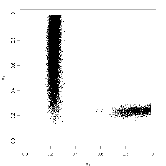
Figure 5: LOH data simulation: marginal scatterplot of $(\pi_{1},\pi_{2})$.

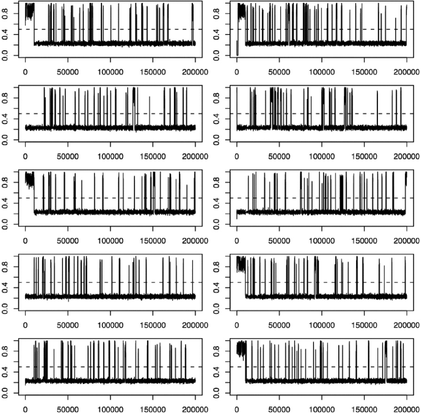
Figure 6: LOH data: parallel traces of $\pi_{1}$. Dotted horizontal line separates the two modes.

Figure 7: LOH data simulation: slices of final RAPTOR boundaries estimates for values of $\eta$ and $\gamma$ equal to their mean in region 1 (left), region 2 (center), whole state space (right). Horizontal axis: $\pi_{1}$; vertical axis: $\pi_{2}$. Dark gray: region 1; light gray: region 2.

In table 5 we summarize final RAPTOR estimates on the original scales, and compare them with the results reported in Craiu et al. (2008). In this table we can see that the results are quite similar, despite the different definitions of the boundary between the two regions. This is probably due to the fact that the two posterior modes are separated by a relatively large region of low probability, so that a certain degree of variability in the boundary specification is allowed, without affecting the results too much. However, it must be noted here again that RAPTOR carries the advantage that the boundary has been learned automatically, with no prior information input.

	$S^{1}$	$S^{2}$	whole space
$\eta$	0.917	0.042	0.840
$\pi_{1}$	0.227	0.949	0.276
$\pi_{2}$	0.768	0.238	0.690
$\gamma$	12.187	-13.249	10.336

	$S^{1}$	$S^{2}$	whole space
$\eta$	0.897	0.079	0.838
$\pi_{1}$	0.229	0.863	0.275
$\pi_{2}$	0.714	0.237	0.679
$\gamma$	15.661	-14.796	13.435

Table 5: Simulation results for LOH data. Region specific and global parameters means for RAPTOR (left) and RAPT (right).

6 Conclusions

We propose a mixture-based approach for regional adaptation of the random walk Metropolis algorithm. Using the theoretical foundations laid by Andrieu and Moulines (2006) we use the online EM algorithm to adapt the parameters of a Gaussian mixtures using the stream of data produced by the MCMC algorithms. In turn, the mixture approximation is used within the regional adaptation paradigm defined by Craiu et al. (2008). The main purpose of the current work is to provide a general method for defining a relatively accurate partition of the sample space. Our simulations suggest that the approach produces partitions that are very close to the optimal one.

A The Online EM algorithm

In the following, we will show how the Online EM algorithm presented in Andrieu and Moulines (2006) applies to the RAPTOR implementation presented in section 3.3.

Consider the following exponential family mixture model (cfr. Andrieu and Moulines (2006), pag. 1488):

$$f_{\eta}(x,z)=\exp\{-\psi(\eta)+\langle T(x,z),\phi(\eta)\rangle\}\quad(\eta,x,z)\in\Omega\times\mathcal{X}\times\mathcal{Z}$$ (A-1)

where the density $f_{\eta}$ is defined w.r.t. some convenient measure on $\Omega\times\mathcal{X}\times\mathcal{Z}$. $T(x,z)$ is the complete data sufficient statistic, i.e. the likelihood $f_{\eta}$ is a function of the complete data pair $(x,z)$ only through the statistic $T(x,z)$. Denote with $\tilde{q}_{\eta}(x)$ the marginal density of $f_{\eta}$:

$$\tilde{q}_{\eta}(x)=\int_{\mathcal{Z}}f_{\eta}(x,z)\mu(dz)$$ (A-2)

One special case of (A-1) is the finite mixture of Gaussians:

$$f_{\eta}(x,z)=\prod_{k=1}^{K}\left[\beta_{\eta}^{k}N(x;\mu_{\eta}^{k},\Sigma_{\eta}^{k})\right]^{\mathbf{1}(z=k)}$$ (A-3)

It can be verified that (A-3) is indeed a special case of (A-1) where $T(x,z)$ takes the form:

$$T(x,z)=\{\mathbf{1}\{z=k\}\cdot(1,\;x,\;xx^{T}),\quad k=1,\ldots,K\}$$ (A-4)

In the above, $x$ denotes a column vector of dimension $d$ and $xx^{T}$ is the usual matrix product. The marginal density $\tilde{q}_{\eta}(x)$ takes the well known form:

$$\tilde{q}_{\eta}(x)=\sum_{k=1}^{K}\beta_{\eta}^{k}N(x;\mu_{\eta}^{k},\Sigma_{\eta}^{k})$$ (A-5)

The central point in the classical EM algorithm is estimating the expected value of the complete log-likelihood (A-1) conditional on $X$ and a value $\eta^{\prime}$ of $\eta$. Thus we need to estimate

$$\mathbb{E}\{\text{log}(f_{\eta}(X,Z))|X,\eta^{\prime}\}$$ (A-6)

Since the complete log-likelihood is linear in $T(X,Z)$ this reduces to computing the conditional expected value of the sufficient statistic. We start by deriving the conditional distribution of $Z$ given $X$ and $\eta$:

$$\nu_{\eta}(x,z) :=\frac{f_{\eta}(x,z)}{\tilde{q}_{\eta}(x)}$$ (A-7)

$$=\frac{\beta_{\eta}^{z}N(x;\mu_{\eta}^{z},\Sigma_{\eta}^{z})}{\sum_{k=1}^{K}\beta_{\eta}^{k}N(x;\mu_{\eta}^{k},\Sigma_{\eta}^{k})}$$

Now we can define:

$$\nu_{\eta}T(x) :=\int_{\mathcal{Z}}T(x,z)\nu_{\eta}(x,z)\mu(dz)$$ (A-8)

$$=\sum_{k=1}^{K}\nu_{\eta}(x,k)\;T(x,k)$$

which is the expected value of the complete data sufficient statistic given $X$ and $\eta$. This can be estimated recursively by the following stochastic approximation scheme:

$$\theta_{n+1}=(1-\alpha_{n+1})\theta_{n}+\alpha_{n+1}\nu_{\eta_{n}}T(X_{n+1})$$ (A-9)

where $\theta_{n}\in\Theta=T(\mathcal{X},\mathcal{Z})$. The Maximization Step is the same as that in the classical EM setup

$$\beta_{\eta_{n}}^{k} =\theta_{n}^{0,k}$$ (A-10)

$$\mu_{\eta_{n}}^{k} =\frac{\theta_{n}^{1,k}}{\theta_{n}^{0,k}}$$

$$\Sigma_{\eta_{n}}^{k} =\frac{\theta_{n}^{2,k}}{\theta_{n}^{0,k}}-\mu_{\eta_{n}}^{k}\mu_{\eta_{n}}^{k\prime}$$

where we have expressed $\theta$ as:

$$\theta=\{(\theta^{0,k},\;\theta^{1,k},\;\theta^{2,k}),\quad k=1,\ldots,K\}$$ (A-11)

with $\theta^{0,k}\in\mathcal{R}$, $\theta^{1,k}\in\mathcal{R}^{d}$, $\theta^{2,k}\in\mathcal{R}^{d\times d}$. Different choices are possible for the learning weights $\alpha_{n}$. One possibility which guarantees convergence is $\alpha_{n}=n^{-1}$, and this is indeed what is used in the RAPTOR implementation.

References

- Andrieu and Moulines (2006) Andrieu, C. and Moulines, E. (2006). On the ergodicity properties of some adaptive MCMC algorithms. Annals of Applied Probability, 16 1462–1505.
- Andrieu et al. (2005) Andrieu, C., Moulines, E. and Priouret, P. (2005). Stability of stochastic approximation under verifiable conditions. Siam Journal On Control and Optimization, 44 283–312.
- Andrieu and Robert (2001) Andrieu, C. and Robert, C. P. (2001). Controlled MCMC for optimal sampling. Tech. rep., Université Paris Dauphine.
- Barrett et al. (1996) Barrett, M., Galipeau, P., Sanchez, C., Emond, M. and Reid, B. (1996). Determination of the frequency of loss of heterozygosity in esophageal adeno-carcinoma nu cell sorting, whole genome amplification and microsatellite polymorphisms. Oncogene, 12.
- Cappé and Moulines (2009) Cappé, O. and Moulines, E. (2009). Online EM algorithm for latent data models. J. Roy. Statist. Soc. Ser. B In print.
- Chen et al. (2000) Chen, M.-H., Shao, Q.-M. and Ibrahim, J. (2000). Monte Carlo Methods in Bayesian Computation. Springer Verlag.
- Craiu et al. (2008) Craiu, R. V., Rosenthal, J. S. and Yang, C. (2008). Learn from thy neighbor: Parallel-chain adaptive MCMC. Tech. rep., University of Toronto.
- Dempster et al. (1977) Dempster, A. P., Laird, N. M. and Rubin, D. B. (1977). Maximum likelihood from incomplete data via the EM algorithm. J. Roy. Statist. Soc. Ser. B, 39 1–22.
- Desai (2000) Desai, M. (2000). Mixture Models for Genetic changes in cancer cells. Ph.D. thesis, University of Washington.
- Haario et al. (2001) Haario, H., Saksman, E. and Tamminen, J. (2001). An adaptive Metropolis algorithm. Bernoulli, 7 223–242.
- Haario et al. (2005) Haario, H., Saksman, E. and Tamminen, J. (2005). Componentwise adaptation for high dimensional MCMC. Computational Statistics, 20 265–273.
- Neal (2001) Neal, R. M. (2001). Annealed importance sampling. Stat. Comput., 11 125–139.
- Roberts et al. (1997) Roberts, G. O., Gelman, A. and Wilks, W. (1997). Weak convergence and optimal scaling of random walk Metropolis algorithms. Ann. Appl. Probab., 7 110–120.
- Roberts and Rosenthal (2001) Roberts, G. O. and Rosenthal, J. S. (2001). Optimal scaling for various Metropolis-Hastings algorithms. Statist. Sci., 16 351–367.
- Roberts and Rosenthal (2006) Roberts, G. O. and Rosenthal, J. S. (2006). Examples of adaptive MCMC. Tech. rep., University of Toronto.
- Roberts and Rosenthal (2007) Roberts, G. O. and Rosenthal, J. S. (2007). Coupling and ergodicity of adaptive Markov chain Monte Carlo algorithms. J. Appl. Probab., 44 458–475.
- Sen and Singer (1993) Sen, P. K. and Singer, J. (1993). Large Sample Methods in Statistics. Wiley: New York.
- Sminchisescu and Triggs (2001) Sminchisescu, C. and Triggs, B. (2001). Covariance-scaled sampling for monocular 3D body tracking. In IEEE International Conference on Computer Vision and Pattern Recognition, vol. 1. Hawaii, 447–454.
- Sminchisescu and Triggs (2002) Sminchisescu, C. and Triggs, B. (2002). Hyperdynamics importance sampling. In European Conference on Computer vision, vol. 1. Copenhagen, 769–783.
- Titterington et al. (1985) Titterington, D. M., Smith, A. F. M. and Makov, U. (1985). Statistical analysis of finite mixture distributions. Wiley, Chichester.
- Warnes (2001) Warnes, G. (2001). The Normal kernel coupler: An adaptive Markov chain Monte Carlo method for efficiently sampling from multi-modal distributions. Tech. rep., George Washington University.