Multi-agent Q-Learning of Channel Selection in Multi-user Cognitive Radio Systems:
A Two by Two Case

Abstract

Resource allocation is an important issue in cognitive radio systems. It can be done by carrying out negotiation among secondary users. However, significant overhead may be incurred by the negotiation since the negotiation needs to be done frequently due to the rapid change of primary users’ activity. In this paper, a channel selection scheme without negotiation is considered for multi-user and multi-channel cognitive radio systems. To avoid collision incurred by non-coordination, each user secondary learns how to select channels according to its experience. Multi-agent reinforcement leaning (MARL) is applied in the framework of Q-learning by considering the opponent secondary users as a part of the environment. The dynamics of the Q-learning are illustrated using Metrick-Polak plot. A rigorous proof of the convergence of Q-learning is provided via the similarity between the Q-learning and Robinson-Monro algorithm, as well as the analysis of convergence of the corresponding ordinary differential equation (via Lyapunov function). Examples are illustrated and the performance of learning is evaluated by numerical simulations.

I Introduction

In recent years, cognitive radio has attracted extensive studies in the community of wireless communications. It allows users without license (called secondary users) to access licensed frequency bands when the licensed users (called primary users) are not present. Therefore, the cognitive radio technique can substantially alleviate the problem of under-utilization of frequency spectrum [11][10].

The following two problems are key to the cognitive radio systems:

• Resource mining, i.e. how to detect the available resource (the frequency bands that are not being used by primary users); usually it is done by carrying out spectrum sensing.

• Resource allocation, i.e. how to allocate the detected available resource to different secondary users.

Substantial work has been done for the resource mining. Many signal processing techniques have been applied to sense the frequency spectrum [17], e.g. cyclostationary feature [5], quickest change detection [8], collaborative spectrum sensing [3]. Meanwhile, plenty of researches have been conducted for the resource allocation in cognitive radio systems [12] [6]. Typically, it is assumed that the secondary users exchange information about detected available spectrum resources and then negotiate the resource allocation according to their own requirements of traffic (since the same resource cannot be shared by different secondary users if orthogonal transmission is assumed). These studies typically apply theories in economics, e.g. game theory, bargaining theory or microeconomics.

However, in many applications of cognitive radio, such a negotiation based resource allocation may incur significant overhead. In traditional wireless communication systems, the available resource is almost fixed (even if we consider the fluctuation of channel quality, the change of available resource is still very slow and thus can be considered stationary). Therefore, the negotiation need not be carried out frequently and the negotiation result can be applied for a long period of data communication, thus incurring tolerable overhead. However, in many cognitive radio systems, the resource may change very rapidly since the activity of primary users may be highly dynamic. Therefore, the available resource needs to be updated very frequently and the data communication period should be fairly short since minimum violation to primary users should be guaranteed. In such a situation, the negotiation of resource allocation may be highly inefficient since a substantial portion of time needs to be used for the negotiation. To alleviate such an inefficiency, high speed transceivers need to be used to minimize the time consumed on negotiation. Particularly, the turn-around time, i.e. the time needed to switch from receiving (transmitting) to transmitting (receiving) should be very small, which is a substantial challenge to hardware design.

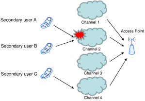
Figure 1: Illustration of competition and conflict in multi-user and multi-channel cognitive radio systems.

Motivated by the previous discussion and observation, in this paper, we study the problem of spectrum access without negotiation in multi-user and multi-channel cognitive radio systems. In such a scheme, each secondary user senses channels and then choose an idle frequency channel to transmit data, as if no other secondary user exists. If two secondary users choose the same channel for data transmission, they will collide with each other and the data packets cannot be decoded by the receiver(s). Such a procedure is illustrated in Fig. 1, where three secondary users access an access point via four channels. Since there is no mutual communication among these secondary users, conflict is unavoidable. However, the secondary users can try to learn how to avoid each other, as well as channel qualities (we assume that the secondary users have no a priori information about the channel qualities), according to its experience. In such a context, the cognition procedure includes not only the frequency spectrum but also the behavior of other secondary users.

To accomplish the task of learning channel selection, multi-agent reinforcement learning (MARL) [1] is a powerful tool. One challenge of MARL in our context is that the secondary users do not know the payoffs (thus the strategy) of each other in each stage; thus the environment of each secondary user, including its opponents, is dynamic and may not assure convergence of learning. In such a situation, fictitious play [2][14], which estimates other users’ strategy and plays the best response, can assure convergence to a Nash equilibrium point within certain assumptions. As an alternative way, we adopt the principle of Q-learning, i.e. evaluating the values of different actions in an incremental way. For simplicity, we consider only the case of two secondary users and two channels. By applying the theory of stochastic approximation [7], we will prove the main result of this paper, i.e. the learning converges to a stationary point regardless of the initial strategies (Propositions 1 and 2 ). Note that our study is one extreme of the resource allocation problem since no negotiation is considered while the other extreme is full negotiation to achieve optimal performance. It is interesting to study the intermediate case, i.e. limited negotiation for resource allocation. However, it is beyond the scope of this paper.

The remainder of this paper is organized as follows. In Section II, the system model is introduced. The proposed Q-learning for channel selection is explained in Section III. Intuitive explanation and rigorous proof for convergence are explained in Sections IV and V, respectively. The numerical results are provided in Section VI while the conclusions are drawn in Section VII.

II System Model

For simplicity, we consider only two secondary users, denoted by $A$ and $B$, and two channels, denoted by 1 and 2. The reward to secondary user $i$, $i=A,B$, of channel $j$, $j=1,2$, is $R_{ij}$ if secondary user transmits data over channel $j$ and channel $j$ is not interrupted by primary user or the other secondary user; otherwise the reward is 0 since the secondary user cannot convey any information over this channel. For simplicity, we denote by $j^{-}$ the other user (channel) different from user (channel) $j$.

The following assumptions are placed throughout this paper.

• The rewards $\{R_{ij}\}$ are unknown to both secondary users. They are fixed throughout the game.

• Both secondary users can sense both channels simultaneously, but can choose only one channel for data transmission. It is more interesting and challenging to study the case that the secondary users can sense only one channel, thus forming a partially observable game. However, it is beyond the scope of this paper.

• We consider only the case that both channels are available since the actions that the secondary users can take are obvious (transmit over the only available channel or not transmit if no channel is available). Thus, we ignore the task of sensing the frequency spectrum, which has been well studied by many researchers, and focus on only the cognition of the other secondary user’s behavior.

• There is no communication between the two secondary users.

III Game and $Q$-learning

In this section, we introduce the corresponding game and the application of Q-learning to the channel selection problem.

III-A Game of Channel Selection

The channel selection problem is a $2\times 2$ game, in which the payoff matrices are given in Fig. 2. Note that the actions, denoted by $a_{i}(t)$ for user $i$ at time $t$, in the game are the selections of channels. Obviously, the diagonal elements in the payoff matrices are all zero since conflict incurs zero reward.

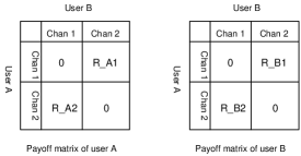
Figure 2: Payoff matrices in the game of channel selection.

It is easy to verify that there are two Nash equilibrium points in the game, i.e. the strategies such that unilaterally changing strategy incurs its own performance degradation. Both equilibrium points are pure, i.e. $a_{A}=1,a_{B}=2$ and $a_{A}=2,a_{B}=1$ (orthogonal transmission).

III-B $Q$-function

Since we assume that both channels are available, then there is only one state in the system. Therefore, the $Q$-function is simply the expected reward of each action (note that, in traditional learning in stochastic environment, the $Q$-function is defined over the pair of state and action), i.e.

$$Q(a)=E[R(a)],$$ (1)

where $a$ is the action, $R$ is the reward dependent on the action and the expectation is over the randomness of the other user’s action. Since the action is the selection of channel, we denote by $Q_{ij}$ the value of selecting channel $j$ by secondary user $i$.

III-C Exploration

In contrast to fictitious play [2], which is deterministic, the action in $Q$-learning is stochastic to assure that all actions will be tested. We consider Boltzmann distribution for random exploration, i.e.

$$P(\mbox{user $i$ choose channel $j$})=\frac{e^{Q_{ij}/\gamma}}{e^{Q_{ij}/\gamma}+e^{Q_{ij^{-}}/\gamma}},$$ (2)

where $\gamma$ is called temperature, which controls the frequency of exploration.

Obviously, when secondary user $i$ selects channel $j$, the expected reward is given by

$$E\left[R_{i}(j)\right]=\frac{R_{ij}e^{Q_{i^{-}j^{-}}/\gamma}}{e^{Q_{i^{-}j}/\gamma}+e^{Q_{i^{-}j^{-}}/\gamma}},$$ (3)

since secondary user $i^{-}$ chooses channel $j$ with probability $\frac{e^{Q_{i^{-}j}/\gamma}}{e^{Q_{i^{-}j}/\gamma}+e^{Q_{i^{-}j^{-}}/\gamma}}$ (collision happens and secondary user $i$ receives no reward) and channel $j^{-}$ with probability $\frac{e^{Q_{i^{-}j^{-}}/\gamma}}{e^{Q_{i^{-}j}/\gamma}+e^{Q_{i^{-}j^{-}}/\gamma}}$ (the transmissions are orthogonal and secondary user $i$ receives reward $R_{ij}$).

III-D Updating $Q$-Functions

In the procedure of $Q$-learning, the $Q$-functions are updated after each spectrum access via the following rule:

$$Q_{ij}(t+1)=(1-\alpha_{ij})Q_{ij}(t)+\alpha_{ij}(t)r_{i}(t)I(a_{i}(t)=j),$$ (4)

where $\alpha_{ij}(t)$ is a step factor (when channel $j$ is not selected by user $i$, $\alpha_{ij}(t)=0$) and $r_{i}(t)$ is the reward of secondary user $i$ and $I$ is characteristic function for the event that channel $j$ is selected at the $t$-th spectrum access. Our study is focused on the dynamics of (4). To assure convergence, we assume that

$$\sum_{t=1}^{\infty}\alpha_{ij}(t)=\infty,\qquad\forall i=A,B,j=1,2.$$ (5)

IV Intuition on Convergence

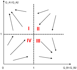
Figure 3: Illustration of the dynamics in the Q-learning.

As will be shown in Propositions 1 and 2, the updating rule of $Q$ functions in (4) will converge to a stationary equilibrium point close to Nash equilibrium if the step factor satisfies certain conditions. Before the rigorous proof, we provide an intuitive explanation for the convergence using the geometric argument proposed in [9].

The intuitive explanation is provided in Fig. 3 (we call it Metrick-Polak plot since it was originally proposed by A. Metrick and B. Polak in [9]), where the axises are $\mu_{A}=\frac{Q_{A1}}{Q_{A2}}$ and $\mu_{B}=\frac{Q_{B1}}{Q_{B2}}$, respectively. As labeled in the figure, the plane is divided into four regions by two lines $\mu_{A}=1$ and $\mu_{B}=1$, in which the dynamics of $Q$-learning are different. We discuss these four regions separately:

• Region I: in this region, $Q_{A1}>Q_{A2}$; therefore, secondary user $A$ prefers visiting channel 1; meanwhile, secondary user $B$ prefers accessing channel 2 since $Q_{B1}>Q_{B2}$; then, with large probability, the strategies will converge to the Nash equilibrium point in which secondary users $A$ and $B$ access channels 1 and 2, respectively.

• Region II: in this region, both secondary users prefer accessing channel 1, thus causing many collisions. Therefore, both $Q_{A1}$ and $Q_{B1}$ will be reduced until entering either region I or region III.

• Region III: similar to region I.

• Region IV: similar to region II.

Then, we observe that the points in Regions II and IV are unstable and will move into Region I or III with large probability. In Regions I and III, the strategy will move close to the Nash equilibrium points with large probability. Therefore, regardless where the initial point is, the updating rule in (4) will generate a stationary equilibrium point with large probability.

V Stochastic Approximation Based Convergence

In this section, we prove the convergence of the $Q$-learning. First, we find the equivalence between the updating rule (4) and Robbins-Monro iteration [13] for solving an equation with unknown expression. Then, we apply the conclusion in stochastic approximation [7] to relate the dynamics of the updating rule to an ordinary differential equation (ODE) and prove the stability of the ODE.

V-A Robbins-Monro Iteration

At a stationary point, the expected values of $Q$-functions satisfy the following four equations:

$$Q_{ij}=\frac{R_{ij}e^{Q_{i^{-}j^{-}}/\gamma}}{e^{Q_{i^{-}j}/\gamma}+e^{Q_{i^{-}j^{-}}/\gamma}},\qquad i=A,B,\mbox{ }j=1,2.$$ (6)

Define $\mathbf{q}=\left(Q_{A1},Q_{A2},Q_{B1},Q_{B2}\right)^{T}$. Then (6) can be rewritten as

$$\mathbf{g}(\mathbf{q})=\mathbf{A}(\mathbf{q})\mathbf{r}-\mathbf{q}=0,$$ (7)

where $\mathbf{r}=\left(R_{A1},R_{A2},R_{B1},R_{B2}\right)^{T}$ and the matrix $\mathbf{A}$ (as a function of $\mathbf{q}$) is given by

$$\mathbf{A}_{ij}=\left\{\begin{array}[]{ll}\frac{e^{Q_{i^{-}j^{-}}/\gamma}}{e^{Q_{i^{-}j}/\gamma}+e^{Q_{i^{-}j^{-}}/\gamma}},&\mbox{ if }i=j\\ 0,&\mbox{ if }i\neq j\end{array}\right..$$ (10)

Then, the updating rule in (4) is equivalent to solving the equation (7) (the expression of the equation is unknown since the rewards, as well as the strategy of the other user, are unknown) using Robbins-Monro algorithm [7], i.e.

$$\mathbf{q}(t+1)=\mathbf{q}(t)+\alpha(t)\mathbf{Y}(t),$$ (11)

where $\mathbf{Y}(t)$ is a random observation on function $g$ contaminated by noise, i.e.

$$\mathbf{Y}(t) = \mathbf{{r}}(t)-\mathbf{q}(t)$$ (12)

$$= \bar{\mathbf{r}}(t)-\mathbf{q}(t)+\mathbf{\hat{r}}(t)-\bar{\mathbf{r}}$$

$$= \mathbf{g}_{t}(\mathbf{q}(t))+\delta M(t),$$

where $\mathbf{g}_{t}(\mathbf{q}(t))=\bar{\mathbf{r}}-\mathbf{q}(t)$, $\delta M(t)=\mathbf{\hat{r}}(t)-\mathbf{q}^{*}$ is noise and (recall that $r_{i}(t)$ means the reward of secondary user $i$ at time $t$)

$$\mathbf{\bar{r}}(t)=\mathbf{A}(\mathbf{q}(t))\mathbf{r}.$$ (13)

V-B ODE and Convergence

The procedure of using Robbins-Monro algorithm (i.e. the updating of $Q$-function) is the stochastic approximation of the solution of the equation. It is well known that the convergence of such a procedure can be characterized by an ODE. Since the noise $\delta M(t)$ in (12) is a Martingale difference, we can verify the conditions in Theorem 12.3.5 in [7] (the verification is omitted due to limited length of this paper) and obtain the following proposition:

Proposition 1

With probability 1, the sequence $\mathbf{q}(t)$ converges to some limit set of the ODE

$$\dot{\mathbf{q}}=\mathbf{g}(\mathbf{q}).$$ (14)

What remains to do is to analyze the convergence property of the ODE (14). We obtain the following proposition:

Proposition 2

The solution of ODE (14) converges to the stationary point determined by (7).

Proof:

We apply Lyapunov’s method to analyze the convergence of the ODE (14). We define the Lyapunov function as

$$V(t) = \|\mathbf{g}(t)\|^{2}$$ (15)

$$= \sum\left(\bar{r}_{ij}(t)-Q_{ij}(t)\right)^{2}.$$

Then, we examine the derivative of the Lyapunov function with respect to time $t$, i.e.

$$\frac{dV(t)}{dt} = 2\sum\frac{d(\bar{r}_{ij}(t)-Q_{ij}(t))}{dt}\left(\hat{r}_{ij}(t)-Q_{ij}(t)\right)$$ (16)

$$= 2\sum\frac{d\epsilon_{ij}(t)}{dt}\epsilon_{ij}(t),$$

where $\epsilon_{ij}(t)\triangleq\hat{r}_{ij}(t)-Q_{ij}(t)$.

We have

$$\frac{d\epsilon_{ij}(t)}{dt} = \frac{d\bar{r}_{ij}(t)}{dt}-\frac{dQ_{ij}(t)}{dt}$$ (17)

$$= \frac{d\bar{r}_{ij}(t)}{dt}-\epsilon_{ij}(t),$$

where $r_{ij}(t)=(\mathbf{A}\mathbf{r})_{ij}$ and we applied the ODE (14).

Then, we focus on the computation of $\frac{dr_{ij}(t)}{dt}$. When $i=A$ and $j=1$, we have

$$\frac{d\bar{r}_{A1}(t)}{dt} = \frac{d}{dt}\left(\frac{R_{A1}e^{Q_{B2}/\gamma}}{e^{Q_{B1}/\gamma}+e^{Q_{B2}/\gamma}}\right)$$ (18)

$$= \frac{R_{A1}e^{Q_{B1}/\gamma}e^{Q_{B2}/\gamma}}{\gamma\left(e^{Q_{B1}/\gamma}+e^{Q_{B2}/\gamma}\right)^{2}}$$

$$\times \left(\frac{dQ_{B2}(t)}{dt}-\frac{dQ_{B1}(t)}{dt}\right)$$

$$= \frac{R_{A1}e^{Q_{B1}/\gamma}e^{Q_{B2}/\gamma}}{\gamma\left(e^{Q_{B1}/\gamma}+e^{Q_{B2}/\gamma}\right)^{2}}$$

$$\times \left(\epsilon_{B2}(t)-\epsilon_{B1}(t)\right),$$

where we applied the ODE (14) again.

Using similar arguments, we have

$$\frac{d\bar{r}_{A2}(t)}{dt} = \frac{R_{A2}e^{Q_{B1}/\gamma}e^{Q_{B2}/\gamma}}{\gamma\left(e^{Q_{B1}/\gamma}+e^{Q_{B2}/\gamma}\right)^{2}}$$ (19)

$$\times \left(\epsilon_{B1}(t)-\epsilon_{B2}(t)\right),$$

and

$$\frac{d\bar{r}_{B1}(t)}{dt} = \frac{R_{B1}e^{Q_{A1}/\gamma}e^{Q_{A2}/\gamma}}{\gamma\left(e^{Q_{A1}/\gamma}+e^{Q_{A2}/\gamma}\right)^{2}}$$ (20)

$$\times \left(\epsilon_{A2}(t)-\epsilon_{A1}(t)\right),$$

and

$$\frac{d\bar{r}_{B2}(t)}{dt} = \frac{R_{B2}e^{Q_{A1}/\gamma}e^{Q_{A2}/\gamma}}{\gamma\left(e^{Q_{A1}/\gamma}+e^{Q_{A2}/\gamma}\right)^{2}}$$ (21)

$$\times \left(\epsilon_{A1}(t)-\epsilon_{A2}(t)\right).$$

Combining the above results, we have

$$\frac{1}{2}\frac{dV(t)}{dt} = -\sum\epsilon_{ij}^{2}(t)$$ (22)

$$+ C_{12}\epsilon_{A1}\epsilon_{B2}-C_{11}\epsilon_{A1}\epsilon_{B1}$$

$$+ C_{21}\epsilon_{A2}\epsilon_{B1}-C_{22}\epsilon_{A2}\epsilon_{B2}$$

where

$$C_{12}=\left(\frac{R_{A1}e^{Q_{B1}/\gamma}e^{Q_{B2}/\gamma}}{\gamma\left(e^{Q_{B1}/\gamma}+e^{Q_{B2}/\gamma}\right)^{2}}+\frac{R_{B2}e^{Q_{A1}/\gamma}e^{Q_{A2}/\gamma}}{\gamma\left(e^{Q_{A1}/\gamma}+e^{Q_{A2}/\gamma}\right)^{2}}\right),$$ (23)

and

$$C_{11}=\left(\frac{R_{A1}e^{Q_{B1}/\gamma}e^{Q_{B2}/\gamma}}{\gamma\left(e^{Q_{B1}/\gamma}+e^{Q_{B2}/\gamma}\right)^{2}}+\frac{R_{B1}e^{Q_{A1}/\gamma}e^{Q_{A2}/\gamma}}{\gamma\left(e^{Q_{A1}/\gamma}+e^{Q_{A2}/\gamma}\right)^{2}}\right),$$ (24)

and

$$C_{21}=\left(\frac{R_{A2}e^{Q_{B1}/\gamma}e^{Q_{B2}/\gamma}}{\gamma\left(e^{Q_{B1}/\gamma}+e^{Q_{B2}/\gamma}\right)^{2}}+\frac{R_{B1}e^{Q_{A1}/\gamma}e^{Q_{A2}/\gamma}}{\gamma\left(e^{Q_{A1}/\gamma}+e^{Q_{A2}/\gamma}\right)^{2}}\right),$$ (25)

and

$$C_{22}=\left(\frac{R_{A2}e^{Q_{B1}/\gamma}e^{Q_{B2}/\gamma}}{\gamma\left(e^{Q_{B1}/\gamma}+e^{Q_{B2}/\gamma}\right)^{2}}+\frac{R_{B2}e^{Q_{A1}/\gamma}e^{Q_{A2}/\gamma}}{\gamma\left(e^{Q_{A1}/\gamma}+e^{Q_{A2}/\gamma}\right)^{2}}\right),$$ (26)

It is easy to verify that

$$\frac{e^{Q_{B1}/\gamma}e^{Q_{B2}/\gamma}}{\left(e^{Q_{B1}/\gamma}+e^{Q_{B2}/\gamma}\right)^{2}}<1.$$ (27)

Now, we assume that $R_{ij}<2\gamma$, then $C_{ij}<2$. Therefore, we have

$$\frac{1}{2}\frac{dV(t)}{dt} < -\sum\epsilon_{ij}^{2}(t)+2\epsilon_{A1}\epsilon_{B2}+2\epsilon_{A2}\epsilon_{B1}$$ (28)

$$= -(\epsilon_{A1}-\epsilon_{B2})^{2}-(\epsilon_{A2}-\epsilon_{B1})^{2}<0.$$

Therefore, when $R_{ij}<2\gamma$, the derivative of the Lyapunov function is strictly negative, which implies that the ODE (14) converges to a stationary point.

The final step of the proof is to remove the condition $R_{ij}<2\gamma$. This is straightforward since we notice that the convergence is independent of the scale of the reward $R_{ij}$. Therefore, we can always scale the reward such that $R_{ij}<2\gamma$. This concludes the proof.

∎

VI Numerical Results

In this section, we use numerical simulations to demonstrate the theoretical results obtained in previous sections. For all simulations, we use $\alpha_{ij}(t)=\frac{\alpha_{0}}{t}$, where $\alpha_{0}$ is the initial learning factor.

VI-A Dynamics

Figures 4 and 5 show the dynamics of $\frac{Q_{A1}}{Q_{A2}}$ versus $\frac{Q_{B1}}{Q_{B2}}$ of several typical trajectories. Note that $\gamma=0.1$ in Fig. 4 and $\gamma=0.01$ in Fig. 5. We observe that the trajectories move from unstable regions (II and IV in Fig. 3) to stable regions (I and III in Fig. 3). We also observe that the trajectories for smaller temperature $\gamma$ is smoother since less explorations are carried out.

Fig. 6 shows the evolution of the probability of choosing channel 1 when $\gamma=0.1$. We observe that both secondary users prefer channel 1 at the beginning and soon secondary user $A$ intends to choose channel 2, thus avoiding the collision.

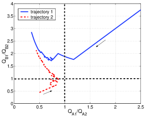
Figure 4: An example of dynamics of the $Q$-learning.

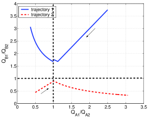
Figure 5: An example of dynamics of the $Q$-learning.

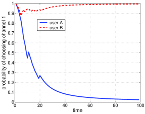
Figure 6: An example of the evolution of channel selection probability.

VI-B Learning Speed

Figures 7 and 8 show the delays of learning (equivalently, the learning speed) for different learning factor $\alpha_{0}$ and different temperature $\gamma$, respectively. The original $Q$ values are randomly selected. When the probabilities of choosing channel 1 are larger than 0.95 for one secondary user and smaller than 0.05 for the other secondary user, we claim that the learning procedure is completed. We observe that larger learning factor $\alpha_{0}$ results in smaller delay while smaller $\gamma$ yields faster learning procedure.

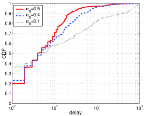
Figure 7: CDF of learning delay with different learning factor $\alpha_{0}$.

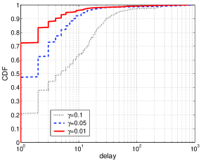
Figure 8: CDF of learning delay with different temperature $\gamma$.

VI-C Fluctuation

In practical systems, we may not be able to use vanishing $\alpha_{ij}(t)$ since the environment could change (e.g. new secondary users emerge or the channel qualities change). Therefore, we need to set a lower bound for $\alpha_{ij}(t)$. Similarly, we also need to set a lower bound for the probability of exploring all actions (notice that the exploration probability in (2) can be arbitrarily small). Fig. 9 shows that the learning procedure may yield substantial fluctuation if the lower bounds are improperly chosen (the lower bounds for $\alpha_{ij}(t)$ and exploration probability are set as 0.4 and 0.2 in Fig. 9).

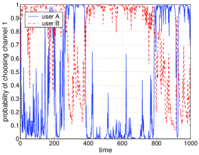
Figure 9: Fluctuation when improper lower bounds are selected.

VII Conclusions

We have discussed the $2\times 2$ case of learning procedure for channel selection without negotiation in cognitive radio systems. During the learning, each secondary user considers the channel and the other secondary user as its environment, updates its $Q$ values and takes the best action. An intuitive explanation for the convergence of learning is provided using Metrick-Polak plot. By applying the theory of stochastic approximation and ODE, we have shown the convergence of learning under certain conditions. Numerical results show that the secondary users can learn to avoid collision quickly. However, if parameters are improperly chosen, the learning procedure may yield substantial fluctuation.

References

- [1] L. Buşoniu, R. Babus̆ka and B. D. Schutter, “A comprehensive survey of multiagent reinforcement learning,” IEEE Trans. Systems, Man and Cybernetics, Part C, vol.38, no.2, pp.156–172, March 2008.
- [2] D. Fudenberg and D. K. Levine, The Theory of Learning in Games. The MIT Press, Cambridge, MA, 1998.
- [3] A. Gahsemi and E. S. Sousa, “Collaborative spectrum sensing for opportunistic access in fading environment,” in Proc. of IEEE International Symposium of New Frontiers in Dynamic Spectrum Access Networks (DySPAN), 2005.
- [4] E. Hossain, D. Niyato and Z. Han, Dynamic Spectrum Access in Cognitive Radio Networks. Cambridge University Press, UK, 2009.
- [5] K. Kim, I. A. Akbar, K. K. Bae, et al, “Cyclostationary approaches to signal detection and classificition in cognitive radio,” in Proc. of IEEE International Symposium of New Frontiers in Dynamic Spectrum Access Networks (DySPAN), April 2007.
- [6] C. Kloeck, H. Jaekel and F. Jondral, “Multi-agent radio resource allocation,” Mobile Networks and Applications, vol. 11, no. 6, Dec. 2006.
- [7] H. J. Kushner and G. G. Yin, Stochastic Approximation and Recursive Algorithms and Applications. Springer, 2003.
- [8] H. Li, C. Li and H. Dai, “Quickest spectrum sensing in cognitive radio,” in Proc. of the 42nd Conference on Information Scicens and Systems (CISS), Princeton, NJ, 2008.
- [9] A. Metrick and B. Polak, “Fictitious play in games: A geometric proof of convergence,” Economic Theory, pp. 923–933, 1994.
- [10] J. Mitola, “Cognitive radio for flexible mobile multimedia communications,” in Proc. IEEE Int. Workshop Mobile Multimedia Communications, pp. 3–10, 1999.
- [11] J. Mitola, “Cognitive Radio,” Licentiate proposal, KTH, Stockholm, Sweden.
- [12] D. Niyato, E. Hossain and Z. Han, “Dynamics of multiple-seller and multiple-buyer spectrum trading in cognitive radio networks: A game theoretic modeling approach,” to appear in IEEE Trans. Mobile Computing.
- [13] H. Robbins and S. Monro, “A stochastic approximation method,” The Annals of Mathematical Statistics, vol. 2, pp. 400–407, 1951.
- [14] J. Robinson, “An iterative method of solving a game,” The Annals of Mathematics, vol. 54, no. 2, pp. 296–301, 1969.
- [15] R. S. Sutton and A. G. Barto, Reinforcement Learning: A Introduction, The MIT Press, Cambridge, MA, 1998.
- [16] C. Watkins, Learning From Delayed Rewards, PhD Theis, The University of Cambridge, UK, 1989.
- [17] Q. Zhao and B. M. Sadler, “A survey of dynamic spectrum access,” IEEE Signal Processing Magazine, vol. 24, pp. 79–89, May. 2007.