Soliton interactions of the Kadomtsev-Petviashvili equation and generation of large-amplitude water waves

 

We study the maximum wave amplitude produced by line-soliton interactions of the Kadomtsev-Petviashvili II (KPII) equation, and we discuss a mechanism of generation of large amplitude shallow water waves by multi-soliton interactions of KPII. We also describe a method to predict the possible maximum wave amplitude from asymptotic data. Finally, we report on numerical simulations of multi-soliton complexes of the KPII equation which verify the robustness of all types of soliton interactions and web-like structure.

 

1. Introduction

The existence of waves of large height on the sea surface is a dangerous phenomenon [12, 17, 21, 27, 33]. Extreme waves occur much more frequently than it might be expected from surface wave statistics [17]. These extreme waves, which are particularly steep and may arise both in deep water and in shallow water, have a significant impact on the safety of people and infrastructure, and are responsible for the erosion of coastlines and sea bottoms and changes to the biological environment. Thus, understanding the physics of these extreme waves is an important task which may even contribute to save lives. Although several physical mechanisms of generation of extreme waves in deep water have been studied, less is known for the situation of shallow water [27].

Waves in shallow water have been studied since the nineteenth century, of course. It is well-known that, in the case of weak nonlinearity, for weakly two-dimensional cases (that is, for the cases that the scale of variation in the direction normal to the propagation direction is much longer than that in the propagation direction) the fundamental equations for the dynamics in shallow water may be reduced to the Kadomtsev-Petviashvili II (KPII) equation [2, 15, 32]. Since the KP equation is integrable, the theory of integrable system can be used to analyze wave dynamics in detail. In particular, Someere et al. recently studied the amplitude of ordinary 2-soliton solutions of the KPII equation[28, 34, 35]. They pointed out that the interaction of two solitary waves may be one mechanism of generation of extreme waves. In the case of ordinary 2-soliton solutions, the maximum interaction height can be four times that of the incoming solitary waves in the limit of the resonant Y-shaped solution originally found by Miles [24, 25, 26]. The interaction pattern of the Miles solution and ordinary 2-soliton solutions, however, is stationary. Therefore, it cannot describe how a large amplitude wave can be generated. Recently, we studied a class of exact line soliton solutions of the KPII equation and found non-stationary interaction patterns and web-like structures [6]. Such solutions describe resonant line-soliton interactions which are generalization of the Y-shaped resonant soliton solution. More general solutions were later characterized in [3, 4, 5, 8, 19].

Our motivation in this paper is severalfold: (i) we determine the maximum amplitude in interactions of line solitons of the KPII equation, (ii) we propose a mechanism to explain the generation of waves of large height, (iii) we describe an algorithm to determine the maximum amplitude from experimental data, (iv) we perform numerical simulations of multi-soliton interactions of the KPII equation, whose results confirm the robustness and stability of soliton interactions and web-like structure.

2. The KPII equation and its soliton solutions

Here we briefly review some essential results the KPII equation

$$(-4u_{t}+6uu_{x}+u_{xxx})_{x}+3u_{yy}=0$$ (2.1)

that will be referred to through the rest of this work. Hereafter, $u(x,y,t)$ represents the dimensionless wave height to leading order, and subscripts $x,y,t$ denote partial differentiation. It is well known that solutions of (2.1) can be expressed via a tau function $\tau(x,y,t)$ as

$$u(x,y,t)=2\frac{\partial^{2}}{\partial x^{2}}\log\tau(x,y,t),$$ (2.2)

where $\tau(x,y,t)$ satisfies Hirota’s bilinear equation [13, 30]. Solutions of Hirota’s equation can be written in terms of the Wronskian determinant [10, 11]

$$\tau(x,y,t)=\mathop{\rm Wr}(f_{1},\cdots,f_{N})=\det(f_{n}^{(n^{\prime}-1)})_{1\leq n,n^{\prime}\leq N}\,,$$ (2.3)

with $f_{n}^{(j)}=\partial^{j}f_{n}/\partial x^{j}$, and where $f_{1},\dots,f_{N}$ are a set of linearly independent solutions of the linear system

$$\frac{\partial f}{\partial y}=\frac{\partial^{2}f}{\partial x^{2}},\,\quad\frac{\partial f}{\partial t}=\frac{\partial^{3}f}{\partial x^{3}}\,.$$ (2.4)

For example, ordinary $N$-soliton solutions are obtained by taking $f_{n}=e^{\theta_{2n-1}}+e^{\theta_{2n}}$ for $n=1,\dots,N$, where

$$\theta_{m}(x,y,t)=-k_{m}x+k_{m}^{2}y-k_{m}^{3}t+\theta_{m;0}\,$$ (2.5)

for $m=1,\dots,2N$, where the $4N$ parameters $k_{1}<\cdots<k_{2N}$ and $\theta_{1;0},\dots,\theta_{2N;0}$ are real constants. For $N=1$, one obtains the single-soliton solution of KPII:

$$u_{i,j}(x,y,t)={\textstyle\frac{1}{2}}a_{i,j}^{2}\mathop{\rm sech}\nolimits^{2}\big{[}{\textstyle\frac{1}{2}}(\theta_{i}-\theta_{j})\big{]}\,,$$ (2.6)

where $i=1$ and $j=2$. Equation (2.6) is a traveling-wave solution, [with wavenumber $\mathbf{k}=(k_{j}-k_{i},k_{i}^{2}-k_{j}^{2})$ and frequency $\omega=k_{i}^{3}-k_{j}^{3}$], exponentially localized along the line $\theta_{i}=\theta_{j}$ of the $xy$-plane, and is therefore referred to as a line soliton. We refer to

$$a_{i,j}=k_{j}-k_{i}\,,\qquad d_{i,j}=k_{i}+k_{j}\,$$ (2.7)

respectively as the soliton amplitude and direction. Note that $d_{i,j}=\tan\alpha_{i,j}$, where $\alpha_{i,j}$ is the angle made by the soliton with the positive $y$-axis (counted clockwise), since $\theta_{i}-\theta_{j}=(k_{i}-k_{j})[-x+d_{i,j}y-(k_{i}^{2}+k_{i}k_{j}+k_{j}^{2})t]+\theta_{i;0}-\theta_{j;0}$. The actual maximum of the solution, or wave height, is given by $U_{i,j}=\frac{1}{2}a_{i,j}^{2}$.

The case with $N=1$ and $f=e^{\theta_{1}}+\cdots+e^{\theta_{M}}$, with $\theta_{1},\dots,\theta_{M}$ still given by (2.5), was studied in [23]. In particular $M=3$ yields the Y-shaped solution often called Miles resonance, in which three line solitons interact at a vertex, as shown in Fig. 2, and whose wavenumbers and phase parameters satisfy the resonance conditions $\mathbf{k}_{1}+\mathbf{k}_{2}=\mathbf{k}_{3}$ and $\omega_{1}+\omega_{2}=\omega_{3}$. (Note that, while the Miles resonance is also a traveling wave solutions, solutions with $M\geq 4$ are not [23].) More in general, choosing $f_{n}=f^{(n-1)}$ for $n=1,\dots,N$ yields $\tau(x,y,t)$ in the form of a Hankel determinant. In [6] we studied such solutions with $f=e^{\theta_{1}}+\cdots+e^{\theta_{M}}$, and we showed that they produce non-stationary and fully resonant $(N_{-},N_{+})$-soliton solutions of KPII, that is, solutions with $N_{-}=M-N$ solitons asymptotically as $y\to-\infty$ and $N_{+}=N$ solitons asymptotically as $y\to\infty$, and for intermediate values of $y$ these solitons interact resonantly, i.e., via fundamental Miles resonances.

It should be clear that even more general solutions exist, however. The most general linear combination of exponentials can be written as

$$f_{n}=\sum_{m=1}^{M}c_{n,m}\,e^{\theta_{m}}\,,$$ (2.8)

with $\theta_{m}$ given by (2.5) as before. Then (2.3) is expanded as a sum of exponentials:

$$\tau(x,y,t)=\det(C\Theta K)=\sum_{1\leq m_{1}<\cdots<m_{N}\leq M}V_{m_{1},\ldots,m_{N}}\,C_{m_{1},\ldots,m_{N}}\,\exp\,\theta_{m_{1},\cdots,m_{N}}\,,$$ (2.9)

where $C=(c_{n,m})$ is the $N\times M$ coefficient matrix, $\Theta={\rm diag}(e^{\theta_{1}},\cdots,e^{\theta_{M}})$, and the $M\times N$ matrix $K$ is given by $K=(k_{m}^{n-1})$. Hereafter, $\theta_{m_{1},\cdots,m_{N}}$ denotes the phase combination $\theta_{m_{1},\cdots,m_{N}}(x,y,t)=\theta_{m_{1}}+\cdots+\theta_{m_{N}}\,$, while $V_{m_{1},\dots,m_{N}}$ is the Vandermonde determinant $V_{m_{1},\dots,m_{N}}=\prod_{1\leq j<j^{\prime}\leq N}(k_{m_{j^{\prime}}}-k_{m_{j}})\,$, and $C_{m_{1},\ldots,m_{N}}$ is the $N\times N$-minor whose $n$-th column is respectively given by the $m_{n}$-th column of the coefficient matrix for $n=1,\dots,N$. The only time dependence in the tau function comes from the exponential phases $\theta_{m_{1},\dots,m_{N}}$. Also, for all $G\in\mathrm{GL}(N,\mathbb{R})$, the coefficient matrices $C$ and $C^{\prime}=G\,C$ produce the same solution of KPII. Thus without loss of generality one can consider $C$ to be in row-reduced echelon form (RREF), which we will do throughout this work. One can also multiply each column of $C$ by an arbitrary positive constant which can be absorbed in the definition of $\theta_{1;0},\dots,\theta_{M;0}$.

Real nonsingular (positive) solutions of KPII are obtained if $k_{1}<\cdots<k_{M}$ and all minors of $C$ are nonnegative. In [4] we showed that, under these assumptions and some fairly general irreducibility conditions on the coefficient matrix, (2.9) produces $(N_{-},N_{+})$-soliton solutions of KPII with $N_{-}=M-N$ and $N_{+}=N$, as in the simpler case of fully resonant solutions. Asymptotic line solitons are given by (2.6) with the indices $i$ and $j$ labeling the phases $\theta_{i}$ and $\theta_{j}$ being swapped in the transition between two dominant phase combinations along the line $\theta_{i}=\theta_{j}$. Asymptotic solitons can thus be uniquely characterized by an index pair $[i,j]$ with $1\leq i<j\leq M$. We call outgoing line solitons those asymptotic as $y\to\infty$ and incoming line solitons those asymptotic as $y\to-\infty$. The index pairs are uniquely identified by appropriate rank conditions on the minors of the coefficient matrix [4]. We also showed in [4] that this decomposition is time-independent, and that the outgoing solitons are identified by pairs $[i_{n}^{+},j_{n}^{+}]$, $n=1,\dots,N$, where $i_{1}^{+},\dots,i_{N}^{+}$ label the $N$ pivot columns of $C$; similarly, the incoming solitons are identified by pairs $[i_{n}^{-},j_{n}^{-}]$, $n=1,\dots,M-N$, where $j_{1}^{-},\dots,j_{M-N}^{-}$ label the $M-N$ non-pivots columns of $C$.

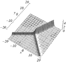
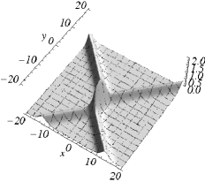
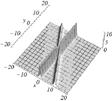
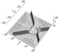
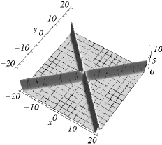
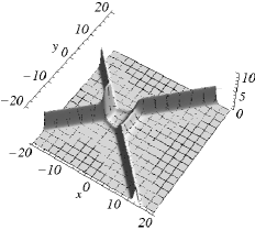
Figure 1: Left: Miles resonance, with $(k_{1},k_{2},k_{3})=(-1,0,1.5)$ and $t=0$. Center: ordinary 2-soliton solution, with $(k_{1},\dots,k_{4})=(-1,-0.001,0,1)$ and $t=0$. Right: asymmetric 2-soliton solution, with $(k_{1},\dots,k_{4})=(-2,-1.5,1,2)$ and $t=0$. In all cases $\theta_{m;0}=0$ for $m=1,\dots,M$.

Figure 2: Time evolution of a resonant 2-soliton solution, with $(k_{1},\dots,k_{4})=(-2,-1,1,2)$ and $\theta_{m;0}=0$ for $m=1,\dots,4$. Left: $t=-3$; center: $t=0$; right: $t=2$.

In general, these solutions exhibit a mixture of resonant and non-resonant interaction patterns. In the special case $M=2N$, leading to $N_{-}=N_{+}=N$, we call elastic $N$-soliton solutions those for which the amplitudes and directions of the incoming solitons coincide with those of the outgoing solitons, while all other $N$-soliton solutions are referred to as inelastic. Elastic $N$-soliton solutions were characterized in [3, 19]. The fully resonant line soliton solutions studied in [6] are a special case of the tau function (2.9) in which all $N\times N$ minors of the coefficient matrix are nonzero.

3. Interaction amplitudes of line-soliton solutions

Here we first study the amplitude generated by 2-soliton interactions. These are obtained for $N=2$ and $M=4$, yielding the tau function

$$\tau(x,y,t)=V_{1,2}C_{1,2}e^{\theta_{1,2}}+V_{1,3}C_{1,3}e^{\theta_{1,3}}+V_{1,4}C_{1,4}e^{\theta_{1,4}}+V_{2,3}C_{1,3}e^{\theta_{2,3}}\\ {}+V_{2,4}C_{1,4}e^{\theta_{2,4}}+V_{3,4}C_{3,4}e^{\theta_{3,4}}\,,$$ (3.1)

where now $V_{i,j}=k_{j}-k_{i}$, and with $k_{1}<\cdots<k_{4}$ as before. The 2-soliton solutions of KPII were recently studied in several papers [7, 19, 4, 5, 8, 9].

3.1. Elastic 2-soliton interactions

It was shown in [19] that elastic 2-soliton solutions are classified into three classes, shown in Figs. 2 and 2: ordinary (O-type), asymmetric (P-type) and resonant (T-type). The coefficient matrices corresponding to these classes have the following RREFs:

$$C_{\rm O}=\left(\!\begin{array}[]{cccc}1&1&0&0\\ 0&0&1&1\\ \end{array}\!\right)\!,\!\quad C_{\rm P}=\left(\!\begin{array}[]{cccc}1&0&0&-1\\ 0&1&1&0\\ \end{array}\!\right)\!,\!\quad C_{\rm T}=\left(\!\begin{array}[]{cccc}1&0&-1&-1\\ 0&1&c_{2,3}&c_{2,4}\\ \end{array}\!\right)\!,$$ (3.8)

with $c_{2,3}>c_{2,4}>0$. These three types of solutions cover disjoint sectors of the 2-soliton parameter space of amplitudes and directions [3]. Moreover, their interaction properties are also different. This difference is obvious in the case of resonant solutions, but also applies to ordinary and asymmetric solutions, since asymmetric solutions only exist for unequal amplitude, and the interaction phase shift has the opposite sign for ordinary and asymmetric solutions [3]. We next show that these solutions also differ in terms of the interaction amplitudes.

Ordinary 2-soliton interactions.

Consider the coefficient matrix $C_{\rm O}$ in (LABEL:e:Aelastic2soliton). It is $C_{1,2}=C_{3,4}=0$ in (3.1), while all other minors are unity. In this case, the dominant phase combination as $x\to-\infty$ is $(2,4)$ [meaning that $e^{\theta_{2,4}}$ is the dominant exponential in (3.1)], while that as $x\to\infty$ is $(1,3)$. The asymptotic solitons are [1,2] and [3,4]. The pattern of this solution is stationary. The maximum height was discussed in [28, 34, 35, 9]. It is expected that the value of $u(x,y,t)$ at the interaction center would give the global maximum. In fact, it was verified in [34]. According to [9], the value of $u(x,y,t)$ at the interaction center, $u_{\rm O}^{\rm(ic)}$, is given by

$$u_{\rm O}^{\rm(ic)}=\frac{1}{2}(a_{1,2}^{2}+a_{3,4}^{2})+a_{1,2}a_{3,4}\,\mbox{tanh}\left(\frac{\varDelta_{\rm O}}{4}\right),$$ (3.10)

where

$$\varDelta_{\rm O}=\log\frac{(k_{3}-k_{1})(k_{4}-k_{2})}{(k_{3}-k_{2})(k_{4}-k_{1})}=\log\frac{(d_{3,4}-d_{1,2})^{2}-(a_{3,4}-a_{1,2})^{2}}{(d_{3,4}-d_{1,2})^{2}-(a_{3,4}+a_{1,2})^{2}}.$$ (3.11)

Since $(k_{3}-k_{1})(k_{4}-k_{2})-(k_{3}-k_{2})(k_{4}-k_{1})=(k_{2}-k_{1})(k_{4}-k_{3})>0$, $\varDelta_{\rm O}>0$. So,

$$\frac{1}{2}(a_{1,2}^{2}+a_{3,4}^{2})<u_{\rm O}^{({\rm ic})}<\frac{1}{2}(a_{1,2}+a_{3,4})^{2}$$ (3.12)

The left hand side is the infinitesimal limit $k_{2}-k_{1}\to 0^{+}$ or $k_{4}-k_{3}\to 0^{+}$ and is the sum of the heights of the asymptotic solitons $U_{1,2}$ and $U_{3,4}$. Accordingly, the maximum height $u_{\rm max}=u_{\rm O}^{({\rm ic})}$ is always greater than the sum of the heights of the asymptotic solitons. It is also lesser than $u_{\rm O}^{(\rm cr)}:=\frac{1}{2}(a_{1,2}+a_{3,4})^{2}$ as long as $k_{1}<k_{2}<k_{3}<k_{4}$. $u_{\rm max}$ takes the critical value $u_{\rm O}^{(\rm cr)}$ in the limit $k_{3}-k_{2}\to 0^{+}$. From $a_{1,2}a_{3,4}\leq(a_{1,2}^{2}+a_{3,4}^{2})/2$, for $a_{1,2}=a_{3,4}=:a$, $u_{\rm O}^{({\rm cr})}$ takes its maximum $2a^{2}=4(a^{2}/2)$ which is four times the height of the incoming solitons. However, it should be noted that in the limit $k_{3}-k_{2}\to 0^{+}$ the solution degenerates to a Y-shape resonant solution.

It is also important to note that since $\frac{1}{2}(a_{1,2}+a_{3,4})^{2}\leq 4(\mbox{max}\{U_{1,2},U_{3,4}\})$ as pointed out in [9], the maximum height of $u(x,y,t)$ is less than four times the height of the taller(tallest) asymptotic soliton.

The right hand side of (3.12) may be also obtained in the following way. Near the critical angle ($k_{2}\approx k_{3}$), the interaction arm appears in the intermediate region of 2 soliton interaction. The interaction arm corresponds to the double-phase transition $(1,3)\leftrightarrow(2,4)$ among the dominant phases in the $xy$-plane, which is located along the line $\theta_{1,3}=\theta_{2,4}$. This is due to the fact that the [1,2]-soliton in $y\to\infty$ is shifted to the right relative to that in $y\to-\infty$, while the [3,4]-soliton in $y\to\infty$ is shifted to the left relative to that in $y\to-\infty$. In a neighborhood of the line corresponding to the double-phase transition $(i_{1},i_{2})\leftrightarrow(j_{1},j_{2})$, the tau function and the corresponding solution of KP are approximately, up to exponentially smaller terms,

$$\tau_{i_{1}i_{2},j_{1}j_{2}}(x,y,t)=V_{i_{1},i_{2}}e^{\theta_{i_{1},i_{2}}}+V_{j_{1},j_{2}}e^{\theta_{j_{1},j_{2}}}\,,$$ (3.13)

$$u_{i_{1}i_{2},j_{1}j_{2}}(x,y,t)={\textstyle\frac{1}{2}}a_{i_{1}i_{2},j_{1}j_{2}}^{2}\mathop{\rm sech}\nolimits^{2}\big{[}{\textstyle\frac{1}{2}}(\theta_{j_{1},j_{2}}-\theta_{i_{1},i_{2}}+\Delta_{i_{1}i_{2},j_{1}j_{2}})\big{]}\,,$$ (3.14)

where $\Delta_{i_{1}i_{2},j_{1}j_{2}}=\log(V_{j_{1},j_{2}}/V_{i_{1},i_{2}})$ and

$$a_{i_{1}i_{2},j_{1}j_{2}}=k_{j_{1}}+k_{j_{2}}-(k_{i_{1}}+k_{i_{2}}).$$ (3.15)

The double-soliton (3.14) is not in itself an exact solution of the KPII equation (and hence it is not a true line soliton), because its wavevector and frequency do not satisfy the soliton dispersion relation [14]. This relation is satisfied in the limit $k_{3}-k_{2}\to 0^{+}$. In this limit there are only three phases in the tau function, and the solution degenerates to a Y-junction. In this limit, the interaction arm of ordinary 2-soliton solutions is given by $u(x,y,t)=u_{13,24}(x,y,t),\ a_{13,24}=a_{1,2}+a_{3,4}$. This result agrees with the right hand side of  (3.12). This method may be, therefore, effective for deriving the supremum for the height of the ordinary 2-soliton solution.

Asymmetric 2-soliton interactions.

Consider now $C_{\rm P}$ in (LABEL:e:Aelastic2soliton). It is $C_{1,4}=C_{2,3}=0$ while all other minors are unity. The asymptotic solitons are [1,4] and [2,3], and the dominant phase combinations as $x\to-\infty$ and $x\to\infty$ are $(3,4)$ and $(1,2)$, respectively. According to [9], the value of $u(x,y,t)$ at the interaction center, $u_{\rm P}^{\rm(ic)}$, is given by

$$u_{\rm P}^{\rm(ic)}=\frac{1}{2}(a_{1,4}^{2}+a_{2,3}^{2})-a_{1,4}a_{2,3}\,\mbox{tanh}\left(\frac{\varDelta_{\rm P}}{4}\right),$$ (3.16)

where

$$\varDelta_{\rm P}=\log\frac{(k_{3}-k_{1})(k_{4}-k_{2})}{(k_{2}-k_{1})(k_{4}-k_{3})}=\log\frac{(a_{1,4}+a_{2,3})^{2}-(d_{1,4}-d_{2,3})^{2}}{(a_{1,4}-a_{2,3})^{2}-(d_{1,4}-d_{2,3})^{2}}>0.$$ (3.17)

Accordingly, we have the estimate

$$\frac{1}{2}(a_{1,4}-a_{2,3})^{2}<u_{\rm P}^{\rm(ic)}\leq\frac{1}{2}a_{1,4}^{2}.$$ (3.18)

The left hand side is the resonance limit $k_{2}-k_{1}\to 0^{+}$ or $k_{4}-k_{3}\to 0^{+}$. The right hand side is the infinitesimal limit $k_{3}-k_{2}\to 0^{+}$. Note that in this limit $a_{2,3}\to 0$. It is also noted that more accurate estimate for right hand side can be obtained (see [9]). Unlike the ordinary 2-soliton solution, $u_{\rm P}^{\rm(ic)}$ does not give the global maximum of $u(x,y,t)$. It is rather given by the height of the highest asymptotic soliton $U_{1,4}=\frac{1}{2}a_{1,4}^{2}$.

The left hand side of (3.18) can be also obtained in the same way as in the ordinary 2-soliton solution. For clarity, let us assume $k_{1}+k_{4}>k_{2}+k_{3}$. In this case, [1,4]-soliton is located on the right side of [2,3]-soliton in $y\to\infty$ as in Fig.2. The [1,4]-soliton in $y\to\infty$ is shifted to the right relative to that in $y\to-\infty$, while the [2,3]-soliton in $y\to\infty$ is shifted to the left relative to that in $y\to-\infty$. Accordingly, the interaction arm appears as the boundary between the two dominant phase regions $(1,3)$ in $y\to-\infty$ and $(2,4)$ in $y\to\infty$. Thus, the amplitude of the interaction arm in the resonance limit $k_{2}-k_{1}\to 0^{+}$ is given by $a_{13,24}$ as for ordinary solutions. Since $a_{13,24}=k_{2}+k_{4}-(k_{1}+k_{3})=k_{4}-k_{1}-(k_{3}-k_{2})=a_{1,4}-a_{2,3}$, this result agrees with the left hand side of (3.18). For $k_{1}+k_{4}<k_{2}+k_{3}$, we can also the same final result.

For $k_{1}+k_{4}=k_{2}+k_{3}$, [1,4] and [2,3] solitons are parallel and one-dimensional over-taking interaction takes place. Even for this case, (3.16) is still valid if we take the interaction center as that in the $(x-(k_{1}+k_{4})y,t)$-plane. According to (3.16), the height at the interaction center is $U_{1,4}-U_{2,3}$.

Resonant 2-soliton interactions.

For the coefficient matrix $C_{\rm T}$ in (LABEL:e:Aelastic2soliton) all minors are nonzero. The dominant phase combinations as $x\to-\infty$ and $x\to\infty$ are respectively $(3,4)$ and $(1,2)$, as with asymmetric solutions, but the asymptotic solitons here are [1,3] and [2,4]. Here the interaction is mediated by four interaction segments and the solution is non-stationary. (Its time evolution is shown in Fig. 2.) Hence, the situation appears at first to be more complicated than in the other two cases. Nonetheless, the calculations are actually simpler, because all the intermediate arms are true line solitons of the KPII equation, and the resonance condition is satisfied at all vertices. Moreover, the interaction pattern obeys the reflection symmetry $(x,y,t)\mapsto(-x,-y,-t)$. Indeed, it would be trivial (however, see the last part of this subsection) to see that, at all times, the tallest intermediate soliton is [1,4], which is obviously taller than either of the asymptotic solitons. Note, however, that $a_{1,3}+a_{2,4}=a_{1,4}+a_{2,3}>a_{1,4}$. Thus the maximum interaction amplitude is always less than the sum of the amplitudes of the asymptotic solitons. In particular, in the case of equal-amplitude solitons, $a_{1,3}=a_{2,4}=:a$, we have $U_{\mathrm{max}}=\frac{1}{2}a_{1,4}^{2}<2a^{2}$. Thus the maximum height is less than four times that of the asymptotic solitons.

Figure 2 shows that the interaction at $t=0$ neither generate the intermediate solitons nor large amplitude. At least, we can prove $u(0,0,0)<\frac{1}{2}a_{1,4}^{2}$ for u(x,y,t) with zero phase constants $\theta_{m;0}=0,m=1,\cdots,4$. Our method is as follows: We express $u(0,0,0)$,which is a function of $k_{i}$, in terms of $d_{i,j}$ and $a_{i,j}$. It turns out that the terms containing $d_{i,j}$ are in the form $(d_{i,j}-d_{m,n})^{2}a_{i,j}a_{m,n}$. Accordingly, all the terms can be expressed in terms of $a_{i,j}$. If we make decomposition like $a_{1,4}=a_{1,2}+a_{2,3}+a_{3,4}$, we find that $\frac{1}{2}a_{1,4}^{2}-u(0,0,0)$ is a sum of positive terms.

3.2. Inelastic 2-soliton interactions

Inelastic 2-soliton solutions fall into four categories [8], identified by the following coefficient matrices in RREF:

$$\begin{array}[]{cc}\displaystyle C_{\rm I}=\left(\!\begin{array}[]{cccc}1&1&0&-r\\ 0&0&1&1\\ \end{array}\!\right)\,,\qquad C_{\rm II}=\left(\!\begin{array}[]{cccc}1&0&-r&-r\\ 0&1&1&1\\ \end{array}\!\right)\,,\\ \displaystyle C_{\rm III}=\left(\!\begin{array}[]{cccc}1&0&0&-r\\ 0&1&1&1\\ \end{array}\!\right)\,,\qquad C_{\rm IV}=\left(\!\begin{array}[]{cccc}1&0&-r&-1\\ 0&1&1&0\\ \end{array}\!\right)\,,\end{array}$$ (3.19)

with $r>0$. We consider each of these in turn. For simplicity in what follows we set $r=1$. Note that in all of these cases exactly one of the minors of $C$ is zero while all other minors are unity, which produces a tau function with five phase combinations.

Type I.

In this case $C_{1,2}=0$. The incoming solitons are [1,2] and [2,4], the outgoing solitons are [1,3] and [3,4]. The dominant phase combination as $x\to-\infty$ is $(3,4)$, while that as $x\to\infty$ is $(1,3)$. The interaction pattern is a combination of two Y-shape resonances, as shown in Figs. 4 and 4. In particular, Fig. 4 shows contour plots of the solution as well as the index pairs corresponding to each of the intermediate and asymptotic solitons. The interaction vertices, however, are not invariant: For $t<0$ the three phases appearing at each interaction vertex are respectively (2,3,4) and (1,2,3), corresponding respectively to solitons [2,3], [3,4], [2,4] and [1,2], [2,3], [1,3]. But at $t=0$ two resonant stems collide, and the arrangement of solitons changes thereafter, with the resonant vertices being characterized by the phases (1,2,4) and (1,3,4) for $t>0$, corresponding respectively to solitons [1,2], [1,4], [2,4] and [1,3], [1,4], [3,4]. (An additional X-shape vertex is produced for $t<0$ by the asymptotic solitons [1,2] and [3,4]. This interaction is locally the ordinary 2-soliton interaction and the local maximum is less than $\frac{1}{2}(a_{1,2}+a_{3,4})^{2}<\frac{1}{2}a_{1,4}^{2}$. We can also prove $u(0,0,0)<\frac{1}{2}a_{1,4}^{2}$ similarly to the case of resonant 2-soliton interactions.)

The rearrangement in the soliton configuration that happens at $t=0$ corresponds to the generation of a large-amplitude wave for $t>0$. The interaction arm is the intermediate soliton [2,3] for $t<0$ and [1,4] for $t>0$. The first of these is always shorter than the asymptotic solitons [1,3] and [2,4]. The second one, however, is taller than any of the others. Moreover, the height of the interaction arm [1,4] is $U_{\mathrm{max}}={\textstyle\frac{1}{2}}a_{1,4}^{2}={\textstyle\frac{1}{2}}(a_{1,j}+a_{j,4})^{2}>{\textstyle\frac{1}{2}}(a_{1,j}^{2}+a_{j,4}^{2})\,$, for $j=2,3$. Thus, the height of the soliton [1,4] is always greater than the sum of the heights of the incoming and the outgoing solitons. As before, the maximum value of the interaction height relative to the height of the asymptotic solitons occurs in the case of equal amplitudes: when $a_{1,2}=a_{2,4}=:a$, it is $U_{\mathrm{max}}=2a^{2}$, yielding a ratio of four to one. However, it should be noted that since $a_{1,3}>a$, $U_{\rm max}$ is less than four times the height of [1,3]-soliton. That is, the maximum height $U_{\rm max}$ is less than four times the height of the highest asymptotic soliton. If we impose still further the condition $a_{1,3}=a_{3,4}=a$, the solution degenerates to a Y-shape resonant solution.

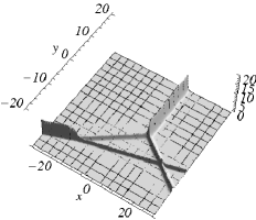
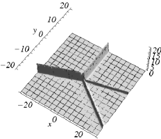
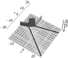
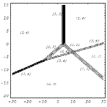
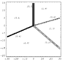
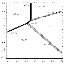
Figure 3: Time evolution of the inelastic 2-soliton solution obtained from the coefficient matrix $C_{\mathrm{I}}$ in (3.19) with $(k_{1},\dots,k_{4})=(-2,0,2,4)$. Left: $t=-2$; center: $t=0$; right: $t=2$.

Figure 4: Contour plots of the inelastic 2-soliton solution shown in Fig. 4. The dominant phase combinations $(m_{1},m_{2})$ and the index pairs $[i,j]$ that uniquely identify the line solitons are labeled. Left: $t=-1$; center: $t=0$; right: $t=1$.

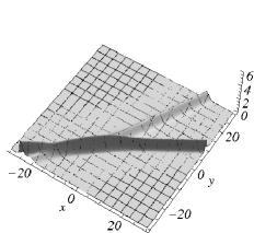
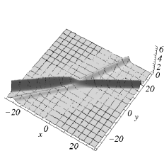
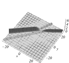
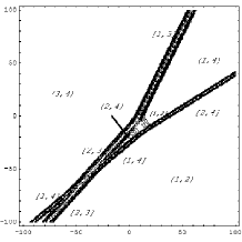
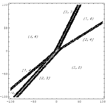
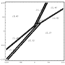
Figure 5: Time evolution of the inelastic 2-soliton solution obtained from $C_{\mathrm{III}}$ in (3.19) with $(k_{1},\dots,k_{4})=(-0.5,-0.1,1,1.7)$. Left: $t=-5$; center: $t=0$; right: $t=5$.

Figure 6: Contour plots of the time evolution of the inelastic 2-soliton solution shown in Fig. 6. Left: $t=-13$; center: $t=0$; right: $t=10$.

Type II.

In this case $C_{3,4}=0$. The incoming solitons are [1,3] and [3,4], the outgoing solitons are [1,2] and [2,4]. The whole solution is a time reversal of the inelastic 2-soliton solution of type I: that is, $u_{\rm II}(x,y,t)=u_{\rm I}(-x,-y,-t)$. The dominant phase combination as $x\to-\infty$ and $x\to\infty$ are now respectively $(2,4)$ and $(1,2)$. The tall interaction arm is still the soliton [1,4], but now it appears for $t<0$.

Type III.

In this case $C_{2,3}=0$. The incoming solitons are [1,4] and [2,3], the outgoing solitons are [1,3] and [2,4]. The dominant phase combination as $x\to-\infty$ is $(3,4)$, while that as $x\to\infty$ is $(1,2)$. The interaction dynamics is similar to that of solutions of type I, as shown in Figs. 6 and 6. The interaction pattern is a combination of two Y-shape resonances. The pattern differs depending on the magnitude relation between $k_{1}+k_{4}$ and $k_{2}+k_{3}$. Figures 6 and 6 show the case $k_{1}+k_{4}>k_{2}+k_{3}$. In this case, for $t<0$, two Y-shape resonances consist of solitons [2,3], [1,3],[1,2] and solitons [1,4],[2,4],[1,2] and for $t>0$, solitons [1,4],[1,3],[3,4] and solitons [2,3],[2,4],[3,4]. For $t<0$, [1,4] and [2,3] solitons make an asymmetric interaction locally. This interaction generates only the height less than the height $U_{1,4}$ of the highest asymptotic soliton. At $t=0$, the exchange of combination of two Y-shape resonances takes place and four solitons interact near the origin of the $xy$-plane. We can again prove $u(0,0,0)<U_{1,4}$ as in the resonance 2-soliton interactions. Accordingly, $U_{1,4}$ is the maximum height in this interaction. For $k_{1}+k_{4}<k_{2}+k_{3}$, the combinations of Y-shape resonances change and an asymmetric interaction of [1,4] and [2,3] solitons takes place for $t>0$. However, the result for the maximum height is the same before. In the case $k_{1}+k_{4}=k_{2}+k_{3}$, [1,4] and [2,3] solitons are parallel and make an over-taking interaction. At $t=0$, these two soliton may coalesce into one peak, the height of which is $U_{1,4}-U_{2,3}$ as described in the subsection on asymmetric 2-soliton interactions, and at the same time the exchange of combination of two Y-shape resonances takes place. So, in this case the maximum height is also $U_{1,4}$.

Type IV.

In this case $C_{1,4}=0$. The incoming solitons are [1,3] and [2,4], the outgoing solitons are [1,4] and [2,3]. Such a solution is a time-reversal version of the inelastic solution of type III: that is, $u_{\rm IV}(x,y,t)=u_{\rm III}(-x,-y,-t)$.

3.3. Generation of large-amplitude waves

None of the three types of elastic 2-soliton solutions describes the generation of large-amplitude waves from the interaction of lower-amplitude ones, since the interaction pattern of ordinary and asymmetric solutions is stationary, and the intermediate soliton [1,4] in resonant solutions is present at all times. On the other hand, inelastic solutions of type I do have the effect of an amplification of the maximum wave height. Moreover, when this kind of solution is embedded in a larger soliton complex, further increases of the wave height may result from the interaction of the interaction arm with the other solitons in the complex. As an example, Fig. 7 shows the large-amplitude wave produced by the interaction generated by the $3\times 6$ coefficient matrix

$$C=\begin{pmatrix}1&1&1&0&0&0\\ 0&0&1&1&0&0\\ 0&0&0&0&1&1\end{pmatrix}\,.$$ (3.20)

As evident from Fig. 7, the interaction among the solitons results in the temporary generation of an extreme wave whose height exceeds four times that of the highest asymptotic soliton.

This discussion suggests the following physical mechanism of generation of extreme waves: (i) several solitons are generated by external sources; (ii) two of those solitons generate a large-height interaction arm, as in the case of ordinary 2-soliton solutions, or that of inelastic solutions of type I; (iii) this interaction arm interacts with one of the other solitons or interaction arms, in which case the wave height can be many times higher that of each asymptotic soliton; (iv) after the interaction, the wave amplitude decreases.

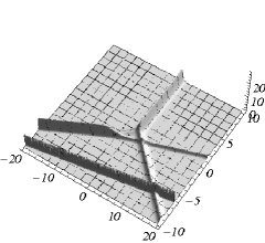
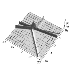
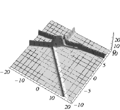
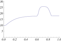
Figure 7: A solution of KP generating an extreme wave, as produced by the coefficient matrix in (3.20) with $(k_{1},\dots,k_{6})=(-2,0,2,4,4.01,8)$, $\theta_{1;0}=\dots\theta_{5;0}=0$ and $\theta_{6;0}=200$. Above, left: $t=-0.4$; above, center: $t=0.7$; above, right: $t=1$. The plot to the right shows the maximum wave height as a function of time.

3.4. A method to predict maximum interaction amplitudes from asymptotic data

The above results yield a method to predict the possible maximum amplitude of a soliton interaction based only on information about the asymptotic line solitons. Consider first the case in which there are two line solitons as $y\to\pm\infty$. Let $(a_{1}^{-},d_{1}^{-})$ and $(a_{2}^{-},d_{2}^{-})$ be the amplitudes and directions of the incoming line solitons, and $(a_{1}^{+},d_{1}^{+})$ and $(a_{2}^{+},d_{2}^{+})$ be those of the outgoing line solitons, both sorted in order of increasing values of $d$. If $d_{1}^{-}=d_{1}^{+}$ or $d_{2}^{-}=d_{2}^{+}$, the incoming and outgoing line solitons coincide, implying that one has an elastic soliton interaction. Otherwise one has an inelastic soliton interaction. For an elastic soliton interaction, the interaction amplitude is computed as follows. Let $\kappa_{n,\pm}=(d_{n}\pm a_{n})/2$ for $n=1,2$. [The superscript $\pm$ in the soliton parameters $a_{n}$ and $d_{n}$ can of course be dropped for elastic solutions.] Then define the phase parameters $k_{1},\dots,k_{4}$ to be the values $\kappa_{1,\pm},\kappa_{2,\pm}$ rearranged in order of increasing size, such that $k_{1}<k_{2}<k_{3}<k_{4}$. In this way each soliton is uniquely identified by the index pair $[i_{n},j_{n}]$ that labels the position of $\kappa_{n,-}$ and $\kappa_{n,+}$ (respectively) in the list $k_{1},\dots,k_{4}$. The type of index overlap determines the type of soliton interaction [3, 8, 19], and the interaction amplitude is then obtained from the calculations described earlier. A similar method applies in the case of an inelastic interaction. In this case, however, one needs the asymptotic data both as $y\to-\infty$ and as $y\to\infty$ in order to uniquely identify the type of interaction.

If the number of solitons is greater than two, one selects any two neighboring solitons and perform the above procedure to compute the possible maximum amplitude. One then repeats these steps for all possible pairwise combinations of solitons. Note, however, that, unlike the case of two solitons, this procedure does not yield a precise estimate, for two reasons: (i) whether or not the theoretical maximum amplitude in each pairwise interaction is realized depends on the details of the soliton configuration; (ii) these high-amplitude intermediate solitons resulting from pairwise interactions can in some cases interact among themselves producing solitons of even higher amplitude. Again, whether or not this happens depends on the details of the soliton configuration. A true upper bound can be obtained: $U_{\mathrm{max}}={\textstyle\frac{1}{2}}(k_{\mathrm{max}}-k_{\mathrm{min}})^{2}$. This theoretical maximum, however, is realized only in a small number of soliton interactions, as should already be evident from the case of 2-soliton solutions.

4. Numerical simulations

We now describe numerical simulations of multi-soliton interactions of the KPII equation. The numerical simulation of multi-soliton solutions is particularly important, since at present no analytical methods exist to investigate the stability of such solutions using either the inverse scattering transform or other techniques.

4.1. A computational method for line-soliton solutions

The numerical integration of the KP equation poses a number of challenges (e.g., see [18] and references therein). In particular, when simulating soliton solutions one must take into account that line solitons are not localized objects, but they extend through the boundaries of any finite computational window. The approach we used here is based on the one in [36, 37, 38, 39, 40], but with different boundary conditions. For the $x$-direction, we set our computational window to be wide enough that any initial solitary waves are far away from boundary. This allows us to use periodic boundary conditions and to compute $x$-derivatives with spectral methods. For the $y$-direction we employ the windowing method [31], which has its roots in signal processing, and where the windowing operation allows the spectral analysis of non-periodic signals. We use the following window function: $W(y)=10^{-a^{n}|2y/L-1|^{n}}\,$, where $L$ is the length of the computational window in the $y$-direction, and $a$ and $n$ are parameters. Here we set $a=1.111$ and $n=27$. We then transform the solution as follows:

$$q(x,y,t)=W(y)\,u(x,y,t)\,,\qquad Q(x,y,t)=W(y)\,u^{2}(x,y,t)\,.$$ (4.1)

Substituting this into the KPII equation, we obtain

$$\big{(}-4q_{t}+3Q_{x}+q_{xxx}\big{)}_{x}+3q_{yy}-6W_{y}u_{y}+3W_{yy}u=0\,.$$ (4.2)

All terms in this equation vanish at the boundaries in the $y$-direction. This makes it possible to apply pseudospectral methods to compute $y$-derivatives. We then integrate (4.2) in time in the Fourier domain using Crank-Nicholson differencing and an iterative method. Once $q(x,y,t)$ is obtained, $u(x,y,t)$ is recovered from (4.1). But note that the formula for $u(x,y,t)$ becomes ill-conditioned near the boundaries in the $y$-direction, where $W(y)$ tends to zero. Near these boundaries, we thus correct the solution using information about the soliton behavior. All the simulations were performed on a grid with $8192\times 1024$ points, $\Delta x=\Delta y=0.1$ and $\Delta t=0.005$. Figures 10–11 below show the resulting field $q(x,y,t)$. Note that, to make the interactions more evident, only a small portion of the computational domain is often shown.

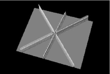
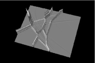
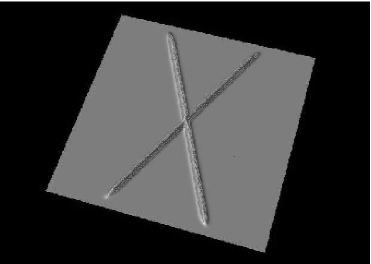
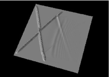
Figure 8: Numerical time evolution of the fully resonant 3-soliton interaction; $(k_{1},\dots,k_{6})=(-2.5,-1.5,-0.5,0.5,1.5,2.5)$. Left: $t=0$; right: $t=10$.

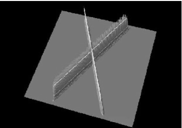
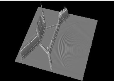
Figure 9: Numerical time evolution of a linear superposition of line solitons generating an ordinary 2-soliton interaction; $(k_{1},\dots,k_{4})=(-1,-0.001,0,1)$. Left: $t=0$; right: $t=50$. The IC is not an exact 2-soliton solution, and some dispersive waves are generated, but the results suggest the stability of the soliton interactions.

Figure 10: Numerical time evolution of a linear superposition of line solitons generating a resonant 2-soliton interaction; $(k_{1},\dots,k_{4})=(-2,-1,1,2)$. Left: $t=0$; right: $t=12.5$. Again, dispersive waves are generated, but the interaction appears to be stable.

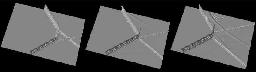
Figure 11: Numerical time evolution of an inelastic 2-soliton interaction. Left: $t=0$; center: $t=2.5$; right: $t=5$.

4.2. Numerical simulations of line-soliton interactions

Figure 10 shows the field $q(x,y,t)$ corresponding to the numerical time evolution of an initial condition (IC) consisting of an exact fully resonant 3-soliton solution. As evident from the figure, the numerical solution accurately reproduces the web structure observed in the exact solution. This result confirms that the numerical method described above can indeed effectively simulate multi-soliton interactions, and at the same time provides a first indication that such solutions are stable.

Next we describe the time evolution of ICs consisting of a linear superposition of two line solitons. Figures 10 and 10 show the cases where the amplitudes and directions were chosen so as to correspond respectively to an ordinary and resonant interaction. We emphasize that, in both cases, the initial state is not an exact two-soliton solution. Indeed, in both cases the numerical solution shows the presence of radiative component of small amplitude. Nonetheless, the results do provide a further check of the stability of 2-soliton interactions. Note in particular that the characteristic “box” of the resonant solution is generated numerically. Similar results were obtained by numerically computing the time evolution of an IC consisting of a linear superposition of two line solitons corresponding to an asymmetric interaction and of three line solitons corresponding to a fully resonant solution. Finally, Fig. 11 shows the time evolution of an IC corresponding to an inelastic interaction.

Importantly, when the IC is not an exact 2-soliton solution, the numerical solutions show that the height of the interaction arm tends monotonically in time to the value for the corresponding exact soliton as obtained in section 3. For example, in Fig. 10 the height of interaction arm increases monotonically in time from its initial value of 2 [owing to an IC that is just a linear superposition of two line solitons], approaching asymptotically the value corresponding to ordinary 2-soliton interactions. Conversely, for an asymmetric solution the height of the interaction arm decreases in time, again approaching asymptotically the value for asymmetric 2-soliton interactions. These results extend the validity and usefulness of the analysis in section 3.

The above results suggest that multi-soliton solutions of KPII are robust and stable, and, moreover, that even when the solution contains non-solitonic components, only the information about the asymptotics line solitons contributes to determine the intermediate interactions of the line solitons. We also suspect that, as the radiative components disperse, asymptotically in time the solution will be closely approximated by an exact soliton solution, similarly to the case of (1+1)-dimensional soliton equations. Of course all of these conjectures must be carefully tested and validated with extensive numerical simulations, which are beyond the scope of this work.

5. Conclusions

We have studied the amplitude of soliton interactions of the KPII equation, and we have discussed a possible mechanism for the generation of large-amplitude waves. Ordinary $N$-soliton interactions with $N\geq 3$ can also briefly produce large amplitude waves if all the solitons intersect simultaneously at the same point in the $xy$-plane. Note however that the event of all solitons intersecting simultaneously at a single point can be considered to be statistically speaking unlikely in a multi-soliton complex, with a likelihood decreasing as the number of solitons increases. In this sense, therefore, the mechanism described in this paper, involving inelastic 2-soliton solutions (possibly embedded in a larger soliton complex, as in Fig. 7) represents the most likely way to generate large-amplitude waves.

We also proposed a method to determine the maximum amplitude resulting from the interaction of two line solitons. The calculation of the maximum amplitude is based on the framework of exact line-soliton solutions, but it may also be useful for solutions where a non-solitonic component is present, if line-soliton solutions of KPII are indeed proven to be stable, since then, even if one starts from an initial state that is not an exact soliton solution, the radiative portions of the solutions will disperse away, and asymptotically in time one will approach a state consisting of an exact soliton solution. An interesting open problem will be to develop an algorithm to compute the actual maximum amplitude generated by any multi-soliton configuration.

Finally, we implemented an algorithm to numerically integrate solutions of the KPII equation containing multi-soliton complexes, and we discussed the results of numerical simulations. These results show the robustness of all types of line-soliton solutions of KPII, including those exhibiting web-like structure. We also confirmed numerically that multi-soliton interactions can generate large amplitude waves, and that an initial state that is not an exact solution eventually converges to an exact multi-soliton solution. We note that resonant 2-soliton solutions with a hole have also been found in other discrete and continuous (2+1)-dimensional soliton equations [14, 16, 20, 22, 36], both in exact solutions and in numerical simulations, indicating that they are a fundamental and robust structure of (2+1)-dimensional soliton equations.

¹ State University of New York, Buffalo, NY, USA
² University of Texas-Pan American, Edinburg, TX, USA
³ Research Institute for Applied Mechanics, Kyushu University, Fukuoka, Japan

Revised Version: Several discussions about amplitude were improved. Several figures were improved. Editorial production errors were corrected.

References

- [1] O
- 2. M. J. Ablowitz and H. Segur, Solitons and the Inverse Scattering Transform (SIAM, Philadelphia, 1981).
- 3. G. Biondini, Phys. Rev. Lett. 99:064103 (2007).
- 4. G. Biondini and S. Chakravarty, J. Math. Phys. 47:033514 (2006).
- 5. G. Biondini and S. Chakravarty, Math. Comp. Sim. 74:237 (2007).
- 6. G. Biondini and Y. Kodama, J. Phys. A 36:10519 (2003).
- 7. M. Boiti, F. Pempinelli, A. K. Pogrebkov and B. Prinari, Inv. Probl. 17:937 (2001).
- 8. S. Chakravarty and Y. Kodama, J. Phys. A 41:275209 (2008).
- 9. S. Chakravarty and Y. Kodama, arXiv:0902.4433v2 (2009).
- 10. N. C. Freeman, Adv. Appl. Mech. 20:1 (1980).
- 11. N. C. Freeman and J. J. C. Nimmo, Phys. Lett. A 95:1 (1983).
- 12. M. Hamer, New Scientist 2201 163:18 (1999).
- 13. R. Hirota, The direct method in soliton theory (Cambridge University Press, Cambridge, 2004).
- 14. E. Infeld and G. Rowlands, Nonlinear waves, solitons and chaos (Cambridge University Press, Cambridge, 2000).
- 15. B. B. Kadomtsev and V. I. Petviashvili, Sov. Phys. Dokl. 15:539 (1970).
- 16. F. Kako and N. Yajima, J. Phys. Soc. Japan 49:2063 (1980).
- 17. C. Kharif and E. Pelinovsky, Euro. J. Mech. B 22:603 (2003).
- 18. C. Klein, C. Sparber and P. Markowich, J. Nonlin. Sci. 17:429 (2007)
- 19. Y. Kodama, J. Phys. A 37:11169. (2004).
- 20. Y. Kodama and K.-i. Maruno, J. Phys. A 39:4063 (2006).
- 21. Y. Li and P.D. Sclavounos, J. Fluid Mech. 470:383 (2002).
- 22. K.-i. Maruno and G. Biondini, J. Phys. A 37:11819 (2004).
- 23. E. Medina, Lett. Math. Phys. 62:91 (2002).
- 24. J. W. Miles, J. Fluid Mech. 79:157 (1977).
- 25. J. W. Miles, J. Fluid Mech. 79:171 (1977).
- 26. M. Oikawa and H. Tsuji, Fluid Dyn. Res. 38:868 (2006).
- 27. E. Pelinovsky, T. Talipova and C. Kharif, Physica D 147:83 (2000).
- 28. P. Peterson, T. Soomere, J. Engelbrecht and E. van Groesen, Nonlin. Proc. Geophys. 10:503 (2003).
- 29. A. V. Porubov, H. Tsuji, I. V. Lavrenov and M. Oikawa, Wave Motion 42:202 (2005).
- 30. J. Satsuma, J. Phys. Soc. Japan 40:286. (1976).
- 31. P. Schlatter, N. A. Adams and L. Kleiser, J. Comp. Phys. 206:505 (2005).
- 32. H. Segur and A. Finkel, Stud. Appl. Math. 73:183 (1985).
- 33. T. Soomere, Env. Fluid Mech. 5:293 (2005).
- 34. T. Soomere, Phys. Lett. A 332:74 (2004).
- 35. T. Soomere and J. Engelbrecht, Wave Motion 41:179 (2005).
- 36. H. Tsuji and M. Oikawa, J. Phys. Soc. Japan 62:3881 (1993).
- 37. H. Tsuji and M. Oikawa, Fluid Dyn. Res. 29:251 (2001).
- 38. H. Tsuji and M. Oikawa, J. Phys. Soc. Japan 73:3034 (2004).
- 39. H. Tsuji and M. Oikawa, J. Phys. Soc. Japan 76:084401 (2007).
- 40. S. B. Wineberg, J. F. McGrath, E. F. Gabl, L. R. Scott and C. E. Southwell, J. Comp. Phys. 97:311 (1991).
1
State University of New York, Buffalo, NY, USA
2
University of Texas-Pan American, Edinburg, TX, USA
3
Research Institute for Applied Mechanics,
Kyushu University, Fukuoka, Japan