Dynamical non-Condon effects in resonant tunneling

Abstract

It is well known that the electron transfer (ET) reaction in donor-bridge-acceptor systems is much influenced by the bridge conformational changes. However, the importance of the dynamical contribution to the ET rate is still under debate. In this study, we investigate the significance of the dynamical non-Condon effect on the ET rate in the coherent resonant tunneling regime. To deal with the resonance, we generalize the time-dependent Fermi’s golden rule expression for the ET rate in the $T$-matrix framework. The dynamical effect is thereby expressed in terms of the time correlation function of the non-Hermitian $T$-matrix. We discuss the property of the quantum time correlation function of the non-Hermitian $T$-matrix and construct the semiclassical approximation. Then we perform a computational study using classical equilibrium molecular dynamics simulations and quantum chemical calculations. It is shown that the ET rate can be significantly enhanced by the dynamical non-Condon effects.

I Introduction

Electron transfer (ET) is one of the most important elementary chemical processes.Nitzan In many cases the simple picture of a direct transfer of an electron from the donor (D) to the acceptor (A) does not apply. Instead, bridge (B) molecules are involved. The standard expression for the ET rate is based on the Condon approximation, in which the dependence of the electronic coupling between D and A on the nuclear configuration is disregarded. However, molecules undergo structural fluctuations over a wide range of timescales at thermal equilibrium. If the B conformational changes influence the electronic coupling, the system will experience a breakdown of the Condon approximation. In the limit of slow electronic coupling fluctuations, the ET rate can be expressed as the ensemble average of the instantaneous ET rate over the static B configuration. This expression captures the structural averaging effect of the B conformation on the electronic coupling, while neglecting the coupling between nuclear and electron dynamics. The dynamical non-Condon effects may become significant as the electronic coupling fluctuations occur on faster timescales.

There have been theoretical developments and computational studies elucidating the dynamical non-Condon effect on the ET rate in the deep (off-resonant) tunneling regime where the energy of the initial electronic state is well separated from the eigenenergies of the B subspace.Tang_JCP93 ; Goychuk_JCP95 ; Daizadeh_PNAS97 ; Medvedev_JCP97 ; Bixon_RJE03 ; Troisi_JCP03 ; Troisi_JACS04 ; Skourtis_PNAS05 ; Nishioka_JPCB05 Starting with the Fermi’s golden rule expression for the ET rate, the dynamical effect is expressed in terms of the time autocorrelation function of the electronic coupling. In a quantum mechanical treatment, the electronic coupling is a Hermitian operator, and its time autocorrelation function satisfies detailed balance. The calculation results in Ref. Medvedev_JCP97, show that for the models of independently coupled bridge modes with coupling of the tunneling electron to the bridge modes, the dynamical non-Condon effects can result in substantial enhancement of the ET rate in the activated inverted region. The detailed balance property is reflected in the asymmetry of the ET rate with respect to the activation energy. On the other hand, the analogous classical time autocorrelation function is a real symmetric function of time and thus does not satisfy detailed balance. Therefore, the classical approximation cannot reproduce the asymmetry of the ET rate due to the dynamical non-Condon effects, but rather produces the symmetric correction to the ET rate with respect to the activation energy, assuming the classical Marcus expression for the Franck-Condon factor.Troisi_JCP03 The enhancement in the activated inverted region is much smaller than that in the quantum mechanical treatment. As pointed out in Ref. Troisi_JCP03, , it is possible to restore detailed balance in the way that the Fourier transform of the classical time autocorrelation function is multiplied by a quantum correction factor. Such semiclassical approximation schemes have been widely discussed over the years.Schofield_PRL60 ; Egelstaff_AP62 ; Berne_JCP67 ; Berne_ACP70 ; An_JCP76 ; Oxtoby_ACP81 ; Berens_JCP81 ; Frommhold ; Bader_JCP94 ; Skinner_JCP97 ; Egorov_CPL98 ; Egorov_JPCA99 ; Skinner_JPCB01 ; Kim_JPCB02

The computational studies have been carried out using classical equilibrium molecular dynamics (MD) simulations and quantum chemical (QC) calculations to evaluate the classical and semiclassical time autocorrelation functions of the electronic coupling.Daizadeh_PNAS97 ; Troisi_JACS04 ; Skourtis_PNAS05 ; Nishioka_JPCB05 The results show that the characteristic timescales for the electronic coupling fluctuations are too slow for the dynamical non-Condon effects to be significant. In the time domain, a comparison between the decay times of the electronic coupling correlation function, and the time-dependent Franck-Condon factor reveals the extent to which dynamical non-Condon effects influence the ET rate. The decay time of the time-dependent Franck-Condon factor is typically $\sim 3-4$ fs.Lockwood_CPL01 On the other hand, the decay time of the electronic coupling correlation function is more than a few tens of fs.Troisi_JACS04 ; Skourtis_PNAS05 ; Nishioka_JPCB05 Therefore, the electronic coupling fluctuations are negligible on the timescale of the decay of the time-dependent Franck-Condon factor. A significantly short decay time of the electronic coupling correlation function was observed only when the electron tunneling energy was artificially brought into resonance with bridge-centered eigenstates.Skourtis_PNAS05 However, there has not ever been confirmation of this statement for a natural system in the resonant tunneling regime.

The purpose of this work is to investigate the timescale of the electronic coupling fluctuations and the possibility of the dynamical non-Condon effects in the resonant tunneling regime through a computational study. We assume that transport is fully coherent, that is, the electron transfers from D to A in a single quantum mechanical process. In the resonant tunneling regime, another contribution comes from sequential tunneling where an electron first tunnels into B and then, after losing its phase memory, tunnels out of B. The dynamical non-Condon effects can substantially increase the contribution from the coherent tunneling, particularly if the B and A electronic states are off resonance. We will consider such situations.

The choice of materials are largely motivated by the previous work for solvent-mediated ET, where B is the solventTroisi_JACS04 . Instead of the C-clamp molecule, we use unlinked D-A systems. In fact, the curved saturated bridge in the C-clamp molecule plays an important role in keeping the distance between D and A. Instead, in this work the D and A molecules are held fixed during the simulation. As an example of the resonant tunneling we consider the ET from the LUMO of naphthalene to the LUMO of tetracyanoethylene (TCNE) in benzonitrile (PhCN). This system lies in the highly activated inverted region (experimental data available for the case of acetonitrile solventRehm_IJC70 ). Therefore, if the electronic coupling fluctuations occur on timescale as short as the decay time of the time-dependent Franck-Condon factor, the dynamical non-Condon effects may cause substantial enhancement of the ET rate.

The Fermi’s golden rule expression refers to the second-order perturbation theory result for the ET rate. In the resonant tunneling regime, higher-order tunneling processes can come into play. In Section II we generalize the Fermi’s golden rule expression to include all high-order tunneling processes in the $T$-matrix framework. The time autocorrelation function of the electronic coupling is thereby replaced by a time correlation function of the $T$-matrix. In practice we will limit our calculations to a small part of a large system, while the effect of the surroundings on the relevant system will be included by broadening the energy levels of the system. In this case the $T$-matrix should be treated as non-Hermitian. In Section III we discuss the properties of the quantum time correlation functions of the $T$-matrix and then describe their semiclassical approximations, which will be used to evaluate the time correlation functions. In Section IV we give the details of the computational methods. In Section V we first show that disregarding the level broadening leads to unacceptable results even in the deep tunneling regime. Then we estimate the level broadening for the charge separation (CS) from the LUMO of anthracene to the LUMO of TCNE and the charge recombination (CR) from the LUMO of TCNE to the HOMO of naphthalene in PhCN, which are in the deep tunneling regime, by comparing the full $T$-matrix results with the second-order perturbation results. Considering the similarities in chemical structure, we expect a similar level broadening for the above-mentioned resonant tunneling process. Taking this into consideration we evaluate the time correlation functions for the resonant tunneling process in Section VI. Then we discuss the significance of the dynamical non-Condon effect on the ET rate. In Section VII we conclude the paper. In Appendix A we sketch the derivation of a level broadening term in the T-matrix formalism.

II $T$-matrix formulation

In the Born-Oppenheimer approximation, the system under consideration can be described by the Hamiltonian

$$\hat{H}_{\mathrm{S}}=(E_{\mathrm{D}}+\hat{H}_{\mathrm{D}})|\mathrm{D}\rangle\langle\mathrm{D}|+(E_{\mathrm{A}}+\hat{H}_{\mathrm{A}})|\mathrm{A}\rangle\langle\mathrm{A}|+\hat{H}_{\mathrm{B}}+(\hat{V}_{\mathrm{AD}}|\mathrm{A}\rangle\langle\mathrm{D}|+\mathrm{h.c.}),$$ (1)

with

$$\hat{H}_{\mathrm{D}}=\sum_{v}E_{\mathrm{D}v}|\mathrm{D}v\rangle\langle\mathrm{D}v|,$$ (2)

$$\hat{H}_{\mathrm{A}}=\sum_{w}E_{\mathrm{A}w}|\mathrm{A}w\rangle\langle\mathrm{A}w|,$$ (3)

$$\hat{H}_{\mathrm{B}}=\sum_{a}E_{a}|a\rangle\langle a|,$$ (4)

$$\hat{V}_{\mathrm{AD}}=\sum_{v,a}\sum_{w,b}V_{\mathrm{A}wb,\mathrm{D}va}|b\rangle|\mathrm{A}w\rangle\langle\mathrm{D}v|\langle a|.$$ (5)

Here $|\mathrm{D}\rangle$ and $|\mathrm{A}\rangle$ are the D and A electronic states, respectively, $|\mathrm{D}v\rangle$ and $|\mathrm{A}w\rangle$ are vibrational states associated with the D and A diabatic energy surfaces, respectively, and $|a\rangle$ and $|b\rangle$ are B vibrational states that modulate only the tunneling barrier between the electronic $|\mathrm{D}\rangle$ and $|\mathrm{A}\rangle$ states. The D and A electronic states depend parametrically on the nuclear coordinates. Because of the fact that the ET occurs only at a specific configuration of the former vibrational modes, the Condon approximation is applicable for them, assuming the local configuration regime. On the other hand, since the latter vibrational modes affect strongly the electronic coupling, the Condon approximation cannot be made. Also, $E_{\mathrm{D}}$ and $E_{\mathrm{A}}$ are the diabatic energy surface bottoms (referred to as the electronic origins) of the D and A states, respectively, $E_{\mathrm{D}v}$ and $E_{\mathrm{A}w}$ are the energies of vibrational states $|\mathrm{D}v\rangle$ and $|\mathrm{A}w\rangle$ measured from the electronic origins, $E_{a}$ is the energy of vibrational state $|a\rangle$, and $V_{\mathrm{D}va,\mathrm{A}wb}$ denotes effective coupling matrix elements between two vibronic states $|\mathrm{D}\rangle|\mathrm{D}v\rangle|a\rangle$ and $|\mathrm{A}\rangle|\mathrm{A}w\rangle|b\rangle$.

The Fermi’s golden rule based expression for the ET rate is given by

$$k_{\mathrm{A}w,b\leftarrow\mathrm{D}v,a}=\frac{2\pi}{\hslash}|\langle\mathrm{A}w,b|\hat{V}_{\mathrm{AD}}|\mathrm{D}v,a\rangle|^{2}\delta(E_{\mathrm{D}}+E_{\mathrm{D}v}+E_{a}-E_{\mathrm{A}}-E_{\mathrm{A}w}-E_{b}),$$ (6)

where $|\mathrm{D}v,a\rangle=|a\rangle|\mathrm{D}v\rangle$, $|\mathrm{A}w,b\rangle=|b\rangle|\mathrm{A}w\rangle$. The Condon approximation for the $|\mathrm{D}v\rangle$ and $|\mathrm{A}w\rangle$ states allows us to write the effective coupling matrix elements between two vibronic states $|\mathrm{D}\rangle|\mathrm{D}v,a\rangle$ and $|\mathrm{A}\rangle|\mathrm{A}w,b\rangle$ as a product of the electronic coupling element $\langle b|\hat{V}_{\mathrm{AD}}|a\rangle$ and the nuclear overlap function $\langle\mathrm{A}w|\mathrm{D}v\rangle$, that is,

$$\langle\mathrm{A}w,b|\hat{V}_{\mathrm{AD}}|\mathrm{D}v,a\rangle=\langle b|\hat{V}_{\mathrm{AD}}|a\rangle\langle\mathrm{A}w|\mathrm{D}v\rangle.$$ (7)

The electronic states can be constructed by using the Hartree-Fock orbitals at fixed nuclear coordinates. The full orbital space is divided into subspaces: the D subspace containing the D orbitals, the A subspace containing the A orbitals, and the B subspace containing the B orbitals. The partitioning Fock matrix is

$$\mathbf{F}=\begin{pmatrix}\mathbf{F}_{\mathrm{DD}}&\mathbf{F}_{\mathrm{DA}}&\mathbf{F}_{\mathrm{DB}}\\ \mathbf{F}_{\mathrm{AD}}&\mathbf{F}_{\mathrm{AA}}&\mathbf{F}_{\mathrm{AB}}\\ \mathbf{F}_{\mathrm{BD}}&\mathbf{F}_{\mathrm{BA}}&\mathbf{F}_{\mathrm{BB}}\end{pmatrix},$$ (8)

e.g., $\mathbf{F}_{\mathrm{AD}}$ is the submatrix of $\mathbf{F}$ with elements $F_{ij}$, where $i$ belongs to the subspace D, and $j$ belongs to the subspace A.

In the deep tunneling regime, within the INDO approximation that we will use, the electronic coupling element between the D and A states is expressed by the effective Fock matrix element defined as

$$\hat{F}_{\mathrm{AD}}^{\mathrm{eff}}=\langle\phi_{\mathrm{A}}|\hat{F}|\phi_{\mathrm{D}}\rangle+\sum_{b_{i}b_{j}}\langle\phi_{\mathrm{A}}|\hat{F}|\phi_{b_{i}}\rangle\langle\phi_{b_{i}}|\frac{1}{E_{\mathrm{tun}}-\hat{F}}|\phi_{b_{j}}\rangle\langle\phi_{b_{j}}|\hat{F}|\phi_{\mathrm{D}}\rangle,$$ (9)

where $\hat{F}$ is the Fock operator, $E_{\mathrm{tun}}$ is the electron tunneling energy, $|\phi_{\mathrm{D}}\rangle$ and $|\phi_{\mathrm{A}}\rangle$ are the D and A orbitals of the tunneling electron, $|\phi_{b_{i}}\rangle$ denotes the intervening B molecular orbitals, and $\sum_{b_{i}}$ refers to a summation over the B orbitals $b_{i}$. Strictly speaking, the effective Fock matrix element should be multiplied by a constant factor dependent on the D and A electronic configurations. We will consider the electronic coupling only between closed-shell Hartree-Fock ground states and singlet spin-adapted configurations that arise as a result of single excitations from them. While the constant factor is $1$ for the coupling between the singly excited electronic configurations, it is $\sqrt{2}$ for between the excited and ground state.

The first and second term in Eq. (9) gives the through-space and through-bridge contribution, respectively. The through-space coupling becomes negligible at the large DA distance discussed below. The coupling matrix element is very much unaffected by the tunneling energy $E_{\mathrm{tun}}$ as long as it remains in the deep tunneling regime. In this case the tunneling energy can be safely varied around the average value of the D and A orbitals. However, this ambiguity becomes a serious problem in the resonant tunneling regime. In particular, the setting, in which the energy denominator in Eq. (9) becomes zero, causes the divergence of the effective Fock matrix element. In the following, we reformulate the ET rate expression in the $T$-matrix framework whereby the tunneling energy is fixed at the initial state energy of the tunneling electron.

The procedure starts by writing the system Hamiltonian as $\hat{H}_{\mathrm{S}}=\hat{H}_{0}+\hat{V}$ with

$$\mathbf{H}_{0}=\begin{pmatrix}\mathbf{F}_{\mathrm{DD}}&\mathbf{0}&\mathbf{0}\\ \mathbf{0}&\mathbf{F}_{\mathrm{AA}}&\mathbf{0}\\ \mathbf{0}&\mathbf{0}&\mathbf{F}_{\mathrm{BB}}\end{pmatrix},$$ (10)

$$\mathbf{V}=\begin{pmatrix}\mathbf{0}&\mathbf{F}_{\mathrm{DA}}&\mathbf{F}_{\mathrm{DB}}\\ \mathbf{F}_{\mathrm{AD}}&\mathbf{0}&\mathbf{F}_{\mathrm{AB}}\\ \mathbf{F}_{\mathrm{BD}}&\mathbf{F}_{\mathrm{BA}}&\mathbf{0}\end{pmatrix},$$ (11)

where $\mathbf{H}_{0}$ and $\mathbf{V}$ are the matrix representation of the operators $\hat{H}_{0}$ and $\hat{V}$, respectively, and $\hat{V}$ is treated as a perturbation to $\hat{H}_{0}$. The eigenstates of the unperturbed Hamiltonian $\hat{H}_{0}$ can be used to construct the D, A, and B orbitals.

Defining the $T$-matrix as

$$\hat{T}=\hat{V}+\hat{V}\,\hat{G}_{\mathrm{S}}(E_{i})\,\hat{V},$$ (12)

with the retarded Green’s function

$$\hat{G}_{\mathrm{S}}(E)=\frac{1}{E-\hat{H}_{\mathrm{S}}+i0^{+}},$$ (13)

one obtains the transition rate from the initial state $|\phi_{i}\rangle$ to the final state $|\phi_{f}\rangle$ as

$$k_{f\leftarrow i}=\frac{2\pi}{\hslash}|\langle\phi_{f}|\hat{T}|\phi_{i}\rangle|^{2}\delta(E_{i}-E_{f}).$$ (14)

Here the two states $|\phi_{i}\rangle$ and $|\phi_{f}\rangle$ are eigenstates of the unperturbed Hamiltonian $\hat{H}_{0}$, and $E_{i}$ and $E_{f}$ are the eigenenergies of states $|\phi_{i}\rangle$ and $|\phi_{f}\rangle$, respectively. We will consider the situation that the initial and final electronic state is described by the D and A orbital $|\phi_{\mathrm{D}}\rangle$ and $|\phi_{\mathrm{A}}\rangle$, respectively. In this case $E_{i}$ and $E_{f}$ are the energies of the the D and A orbitals that will be denoted by $\epsilon_{\mathrm{D}}$ and $\epsilon_{\mathrm{A}}$, respectively. The transition is induced by the perturbation $\hat{V}$ that couples D, A, and B.

Strictly speaking, the nuclear kinetic energy terms should be added to the system Hamiltonian $\hat{H}_{\mathrm{S}}$ because the Fock matrix only contains a contribution from the potential surface for the nuclear motion. Then, the delta function in Eq. (14) can be rewritten in the same form as that in Eq. (6). Assume that the nuclear kinetic energy is the same in the initial and intermediate states to keep the $T$-matrix independent of the nuclear kinetic energies. This assumption seems to be reasonable under the Born-Oppenheimer approximation. Then, keeping in mind that the $T$-matrix is an operator in the space of the B vibrational states, the transition rate can be rewritten in the form

$$k_{\mathrm{A}w,b\leftarrow\mathrm{D}v,a}=\frac{2\pi}{\hslash}|\langle b|\hat{T}_{\mathrm{AD}}|a\rangle|^{2}|\langle\mathrm{A}w|\mathrm{D}v\rangle|^{2}\delta(E_{\mathrm{D}}+E_{\mathrm{D}v}+E_{a}-E_{\mathrm{A}}-E_{\mathrm{A}w}-E_{b}),$$ (15)

with $\hat{T}_{\mathrm{AD}}=\langle\phi_{\mathrm{A}}|\hat{T}|\phi_{\mathrm{D}}\rangle$. In the deep tunneling regime, expansion of the $T$-matrix element $\hat{T}_{\mathrm{AD}}$ to second order in the perturbation $\hat{V}$ gives the effective Fock matrix element $\hat{F}_{\mathrm{AD}}^{\mathrm{eff}}$ with substitution of the D orbital energy $\epsilon_{\mathrm{D}}$ for the tunneling energy $E_{\mathrm{tun}}$. The $T$-matrix includes all higher-order tunneling processes where the initial and final states are coupled by multiple scatterings described by the perturbation $\hat{V}$.

The observed ET rate is given by summing over final vibrational states and thermal averaging over initial vibrational states as

$$k_{\mathrm{A}\leftarrow\mathrm{D}}=\sum_{v,a}P_{\mathrm{D}v}P_{a}\sum_{w,b}k_{\mathrm{A}w,b\leftarrow\mathrm{D}v,a},$$ (16)

where $P_{\mathrm{D}v}$ and $P_{a}$ are the Boltzmann distributions over the vibrational levels $|\mathrm{D}v\rangle$ and $|a\rangle$, respectively. We denote the thermal average over the vibrational states associated with the D diabatic energy surface by $\langle\ldots\rangle_{\mathrm{D}}$, that is, $\langle\ldots\rangle_{\mathrm{D}}=\sum_{v}P_{\mathrm{D}v}\langle\mathrm{D}v|\ldots|\mathrm{D}v\rangle=\mathrm{Tr}_{\mathrm{D}}[e^{-\beta\hat{H}_{\mathrm{D}}}\ldots]/\mathrm{Tr}_{\mathrm{D}}[e^{-\beta\hat{H}_{\mathrm{D}}}]$, where $\beta=(k_{B}T)^{-1}$ and $\mathrm{Tr}_{\mathrm{D}}$ denotes a trace over the eigenstates of $\hat{H}_{\mathrm{D}}$, and the thermal average over the B vibrational states by $\langle\ldots\rangle_{\mathrm{B}}$, that is, $\langle\ldots\rangle_{\mathrm{B}}=\sum_{a}P_{a}\langle a|\ldots|a\rangle=\mathrm{Tr}_{\mathrm{B}}[e^{-\beta\hat{H}_{\mathrm{B}}}\ldots]/\mathrm{Tr}_{\mathrm{B}}[e^{-\beta\hat{H}_{\mathrm{B}}}]$, where $\mathrm{Tr}_{\mathrm{B}}$ denotes a trace over the eigenstates of $\hat{H}_{\mathrm{B}}$. Then, writing the delta function in Eq. (15) as a Fourier transform, we get

$$k_{\mathrm{A}\leftarrow\mathrm{D}}=\frac{1}{\hslash^{2}}\int_{-\infty}^{\infty}d\epsilon\,\tilde{\rho}_{\mathrm{FC}}(E_{\mathrm{D}}-E_{\mathrm{A}}-\epsilon)\,\tilde{C}_{T}(\epsilon/\hslash),$$ (17)

with the thermally averaged Franck-Condon weighted density of states, $\tilde{\rho}_{\mathrm{FC}}$, given by the Fourier transform of the thermally averaged time-dependent Franck-Condon factor

$$\rho_{\mathrm{FC}}(t)\equiv\langle e^{i\hat{H}_{\mathrm{D}}t/\hslash}e^{-i\hat{H}_{\mathrm{A}}t/\hslash}\rangle_{\mathrm{D}},$$ (18)

such that

$$\tilde{\rho}_{\mathrm{FC}}(\epsilon)=\frac{1}{2\pi\hslash}\int_{-\infty}^{\infty}dt\,e^{i\epsilon t/\hslash}\rho_{\mathrm{FC}}(t),$$ (19)

and with the spectral density $\tilde{C}_{T}$ given by the Fourier transform of the time correlation function

$$C_{T}(t)\equiv\langle\hat{T}_{\mathrm{AD}}^{\dagger}(t)\,\hat{T}_{\mathrm{AD}}(0)\rangle_{\mathrm{B}},$$ (20)

where $\hat{T}_{\mathrm{AD}}(t)=e^{i\hat{H}_{\mathrm{B}}t/\hslash}\hat{T}_{\mathrm{AD}}e^{-i\hat{H}_{\mathrm{B}}t/\hslash}$, such that

$$\tilde{C}_{T}(\epsilon/\hslash)=\int_{-\infty}^{\infty}dt\,e^{i\epsilon t/\hslash}C_{T}(t).$$ (21)

Applying the convolution theorem for Fourier transforms, Eq. (17) can be written as

$$k_{\mathrm{A}\leftarrow\mathrm{D}}=\frac{1}{\hslash^{2}}\int_{-\infty}^{\infty}dt\,e^{i(E_{\mathrm{D}}-E_{\mathrm{A}})t/\hslash}\rho_{\mathrm{FC}}(t)\,C_{T}(t).$$ (22)

Note that the $T$-matrix is non-Hermitian due to the infinitesimal term $i0^{+}$. In the deep tunneling regime it is treated as a Hermitian matrix by disregarding the $i0^{+}$ term. However, we will see that in the resonant tunneling regime it is necessary to modify the eigenvalues of $\hat{H}_{\mathrm{S}}$ in the Green’s function (13) to include a finite imaginary term, which represents the effect of the surroundings on the relevant system. Then it is important to deal with the non-Hermitian $T$-matrix. In this case the operator $\hat{T}_{\mathrm{AD}}$ is also non-Hermitian.

III Time correlation functions of $T$-matrix

The non-Hermitian operator $\hat{T}_{\mathrm{AD}}$ can be decomposed into the sum of two Hermitian operators as

$$\hat{T}_{\mathrm{AD}}=\hat{A}+i\hat{B},$$ (23)

where $\hat{A}$ and $\hat{B}$ are Hermitian operators given by

$$\hat{A}=\frac{1}{2}(\hat{T}_{\mathrm{AD}}+\hat{T}_{\mathrm{AD}}^{\dagger}),$$ (24)

$$\hat{B}=\frac{1}{2i}(\hat{T}_{\mathrm{AD}}-\hat{T}_{\mathrm{AD}}^{\dagger}).$$ (25)

Then the quantum time correlation function $C_{T}(t)$ can be separated into the autocorrelation and the cross-correlation part, that is,

$$C_{T}(t)=C_{\mathrm{A}}(t)+iC_{\mathrm{C}}(t),$$ (26)

with

$$C_{\mathrm{A}}(t)=C_{AA}(t)+C_{BB}(t),$$ (27)

$$C_{\mathrm{C}}(t)=C_{AB}(t)-C_{BA}(t),$$ (28)

$$C_{AA}(t)=\langle\hat{A}(t)\,\hat{A}(0)\rangle_{\mathrm{B}},$$ (29)

$$C_{BB}(t)=\langle\hat{B}(t)\,\hat{B}(0)\rangle_{\mathrm{B}},$$ (30)

$$C_{AB}(t)=\langle\hat{A}(t)\,\hat{B}(0)\rangle_{\mathrm{B}},$$ (31)

$$C_{BA}(t)=\langle\hat{B}(t)\,\hat{A}(0)\rangle_{\mathrm{B}},$$ (32)

where

$$\hat{A}(t)=\frac{1}{2}(\hat{T}_{\mathrm{AD}}(t)+\hat{T}_{\mathrm{AD}}^{\dagger}(t)),$$ (33)

$$\hat{B}(t)=\frac{1}{2i}(\hat{T}_{\mathrm{AD}}(t)-\hat{T}_{\mathrm{AD}}^{\dagger}(t)).$$ (34)

These two parts have the following properties:

$$C_{\mathrm{A}}(-t)=C_{\mathrm{A}}^{\ast}(t)=C_{\mathrm{A}}(t-i\beta\hslash),$$ (35)

$$C_{\mathrm{C}}(-t)=-C_{\mathrm{C}}^{\ast}(t)=-C_{\mathrm{C}}(t-i\beta\hslash).$$ (36)

Thus, the Fourier transform

$$\tilde{C}_{\mathrm{A}}(\omega)=\int_{-\infty}^{\infty}dt\,e^{i\omega t}C_{\mathrm{A}}(t)$$ (37)

satisfies the detailed balance relation

$$\tilde{C}_{\mathrm{A}}(\omega)=e^{\beta\hslash\omega}\tilde{C}_{\mathrm{A}}(-\omega),$$ (38)

while the Fourier transform

$$\tilde{C}_{\mathrm{C}}(\omega)=\int_{-\infty}^{\infty}dt\,e^{i\omega t}C_{\mathrm{C}}(t)$$ (39)

does not satisfy detailed balance but

$$\tilde{C}_{\mathrm{C}}(\omega)=-e^{\beta\hslash\omega}\tilde{C}_{\mathrm{C}}(-\omega).$$ (40)

The cross-correlation part represents the nonequilibrium properties of the system. In the deep tunneling regime, $\hat{T}_{\mathrm{AD}}$ is often treated as a Hermitian operator, assuming that the D and A electronic wave functions are real, so that the cross-correlation part vanishes. From Eqs. (35)$-$(39) it follows that $\tilde{C}_{\mathrm{A}}(\omega)$ and $\tilde{C}_{\mathrm{C}}(\omega)$ are real and imaginary, respectively. While $\tilde{C}_{\mathrm{A}}(\omega)\geq 0$, $i\tilde{C}_{\mathrm{C}}(\omega)$ can also be negative. Since the trace is invariant to cyclic permutation of the operators inside it, and the equilibrium density operator $e^{-\beta\hat{H}_{\mathrm{B}}}$ and the time evolution operator $e^{-i\hat{H}_{\mathrm{B}}t/\hslash}$ commute, the quantum time correlation functions are stationary, that is, $\langle\hat{A}(t+t^{\prime})\,\hat{A}(t^{\prime})\rangle_{\mathrm{B}}=\langle\hat{A}(t)\,\hat{A}(0)\rangle_{\mathrm{B}}$, etc.

It will be convenient to decompose $C_{\mathrm{A}}(t)$ and $C_{\mathrm{C}}(t)$ into the real parts

$$C_{\mathrm{A}}^{(+)}(t)=\frac{1}{2}(C_{\mathrm{A}}(t)+C_{\mathrm{A}}^{\ast}(t)),$$ (41)

$$C_{\mathrm{C}}^{(+)}(t)=\frac{1}{2}(C_{\mathrm{C}}(t)+C_{\mathrm{C}}^{\ast}(t)),$$ (42)

and the imaginary parts

$$C_{\mathrm{A}}^{(-)}(t)=\frac{1}{2}(C_{\mathrm{A}}(t)-C_{\mathrm{A}}^{\ast}(t)),$$ (43)

$$C_{\mathrm{C}}^{(-)}(t)=\frac{1}{2}(C_{\mathrm{C}}(t)-C_{\mathrm{C}}^{\ast}(t)).$$ (44)

From Eqs. (35)$-$(39) the Fourier transforms can be written as

$$\tilde{C}_{\mathrm{A}}^{(\pm)}(\omega)=\frac{1}{2}(\tilde{C}_{\mathrm{A}}(\omega)\pm\tilde{C}_{\mathrm{A}}(-\omega)),$$ (45)

$$\tilde{C}_{\mathrm{C}}^{(\pm)}(\omega)=\frac{1}{2}(\tilde{C}_{\mathrm{C}}(\omega)\mp\tilde{C}_{\mathrm{C}}(-\omega)).$$ (46)

While $\tilde{C}_{\mathrm{A}}^{(+)}(\omega)$ and $\tilde{C}_{\mathrm{C}}^{(-)}(\omega)$ are symmetric in $\omega$, $\tilde{C}_{\mathrm{A}}^{(-)}(\omega)$ and $\tilde{C}_{\mathrm{C}}^{(+)}(\omega)$ are antisymmetric in $\omega$. Substitution of Eqs. (38) and (40) into Eqs. (45) and (46) leads to

$$\tilde{C}_{\mathrm{A}}(\omega)=\frac{2}{1\pm e^{-\beta\hslash\omega}}\tilde{C}_{\mathrm{A}}^{(\pm)}(\omega),$$ (47)

$$\tilde{C}_{\mathrm{C}}(\omega)=\frac{2}{1\pm e^{-\beta\hslash\omega}}\tilde{C}_{\mathrm{C}}^{(\pm)}(\omega).$$ (48)

The quantum time correlation function $C_{T}(t)$ can be evaluated using classical equilibrium MD simulations coupled with QC calculations. This approach involves the replacement of the quantum time correlation function by its classical counterpart. We denote the classical time correlation function by

$$C_{T}^{\mathrm{cl}}(t)=\langle T_{\mathrm{AD}}^{\ast}(t)\,T_{\mathrm{AD}}(0)\rangle_{\mathrm{cl}},$$ (49)

with the classical variables

$$T_{\mathrm{AD}}(t)=\langle\phi_{\mathrm{A}}(\mathbf{Q}_{\mathrm{B}}(t))|\hat{T}(\mathbf{Q}_{\mathrm{B}}(t))|\phi_{\mathrm{D}}(\mathbf{Q}_{\mathrm{B}}(t))\rangle,$$ (50)

$$T_{\mathrm{AD}}^{\ast}(t)=\langle\phi_{\mathrm{D}}(\mathbf{Q}_{\mathrm{B}}(t))|\hat{T}^{\dagger}(\mathbf{Q}_{\mathrm{B}}(t))|\phi_{\mathrm{A}}(\mathbf{Q}_{\mathrm{B}}(t))\rangle.$$ (51)

Here, the $T$-matrix $\hat{T}(\mathbf{Q}_{\mathrm{B}}(t))$, and the D and A orbitals $|\phi_{\mathrm{D}}(\mathbf{Q}_{\mathrm{B}}(t))\rangle$ and $|\phi_{\mathrm{A}}(\mathbf{Q}_{\mathrm{B}}(t))\rangle$ are parametric functions of the B nuclear coordinates $\mathbf{Q}_{\mathrm{B}}(t)$ at time $t$ that move along the classical trajectories obtained by the MD simulations, and the classical thermal average $\langle\ldots\rangle_{\mathrm{cl}}$ should be understood as the time average over the MD trajectory, as implied by the ergodic theorem of statistical mechanics.

Using the classical counterparts of $C_{\mathrm{A}}(t)$ and $C_{\mathrm{C}}(t)$, the classical correlation function $C_{T}^{\mathrm{cl}}(t)$ can be written as

$$C_{T}^{\mathrm{cl}}(t)=C_{\mathrm{A}}^{\mathrm{cl}}(t)+iC_{\mathrm{C}}^{\mathrm{cl}}(t),$$ (52)

with

$$C_{\mathrm{A}}^{\mathrm{cl}}(t)=C_{AA}^{\mathrm{cl}}(t)+C_{BB}^{\mathrm{cl}}(t),$$ (53)

$$C_{\mathrm{C}}^{\mathrm{cl}}(t)=C_{AB}^{\mathrm{cl}}(t)-C_{BA}^{\mathrm{cl}}(t),$$ (54)

$$C_{AA}^{\mathrm{cl}}(t)=\langle A(t)\,A(0)\rangle_{\mathrm{cl}},$$ (55)

$$C_{BB}^{\mathrm{cl}}(t)=\langle B(t)\,B(0)\rangle_{\mathrm{cl}},$$ (56)

$$C_{AB}^{\mathrm{cl}}(t)=\langle A(t)\,B(0)\rangle_{\mathrm{cl}},$$ (57)

$$C_{BA}^{\mathrm{cl}}(t)=\langle B(t)\,A(0)\rangle_{\mathrm{cl}},$$ (58)

where

$$A(t)=\frac{1}{2}(T_{\mathrm{AD}}(t)+T_{\mathrm{AD}}^{\ast}(t)),$$ (59)

$$B(t)=\frac{1}{2i}(T_{\mathrm{AD}}(t)-T_{\mathrm{AD}}^{\ast}(t)).$$ (60)

From the time reversal symmetry of the classical equations of motion, it follows that

$$C_{\mathrm{A}}^{\mathrm{cl}}(t)=C_{\mathrm{A}}^{\mathrm{cl}}(-t),$$ (61)

$$C_{\mathrm{C}}^{\mathrm{cl}}(t)=C_{\mathrm{C}}^{\mathrm{cl}}(-t).$$ (62)

Furthermore, the stationary property implies that

$$C_{\mathrm{C}}^{\mathrm{cl}}(-t)=-C_{\mathrm{C}}^{\mathrm{cl}}(t).$$ (63)

Alternatively, taking the classical limit $\hslash\rightarrow 0$, Eq. (36) yields Eq. (63). From Eqs. (62) and (63) it follows that

$$C_{\mathrm{C}}^{\mathrm{cl}}(t)=0.$$ (64)

Namely, the classical approximation disregards the contribution of the cross-correlation part $C_{\mathrm{C}}(t)$ in the time correlation function $C_{T}(t)$.

Using Eqs. (52), (64), (53), (55), (56), (59), and (60) yields

$$C_{T}^{\mathrm{cl}}(t) =C_{\mathrm{A}}^{\mathrm{cl}}(t)=\frac{1}{2}\langle T_{\mathrm{AD}}(t)\,T_{\mathrm{AD}}^{\ast}(0)+T_{\mathrm{AD}}^{\ast}(t)\,T_{\mathrm{AD}}(0)\rangle_{\mathrm{cl}}$$

$$=\langle\mathrm{Re}T_{\mathrm{AD}}(t)\,\mathrm{Re}T_{\mathrm{AD}}(0)\rangle_{\mathrm{cl}}+\langle\mathrm{Im}T_{\mathrm{AD}}(t)\,\mathrm{Im}T_{\mathrm{AD}}(0)\rangle_{\mathrm{cl}}$$

$$\equiv C_{\mathrm{Re}}^{\mathrm{cl}}(t)+C_{\mathrm{Im}}^{\mathrm{cl}}(t),$$ (65)

where $C_{\mathrm{Re}}^{\mathrm{cl}}(t)$ and $C_{\mathrm{Im}}^{\mathrm{cl}}(t)$ define the autocorrelation functions of the real and imaginary parts of $T_{\mathrm{AD}}$, respectively. Since $C_{\mathrm{A}}^{\mathrm{cl}}(t)$ is a real symmetric function of $t$, its Fourier transform

$$\tilde{C}_{\mathrm{A}}^{\mathrm{cl}}(\omega)=\int_{-\infty}^{\infty}dt\,e^{i\omega t}C_{\mathrm{A}}^{\mathrm{cl}}(t)$$ (66)

is a real symmetric function of $\omega$, that is, $\tilde{C}_{\mathrm{A}}^{\mathrm{cl}}(\omega)=\tilde{C}_{\mathrm{A}}^{\mathrm{cl}}(-\omega)$. This means that the classical time correlation function does not satisfy the detailed balance condition (38). The simplest way to solve this problem is to identify $C_{\mathrm{A}}^{\mathrm{cl}}(t)$ with $C_{\mathrm{A}}^{(+)}(t)$. Using the relation (47) we obtain

$$\tilde{C}_{\mathrm{A}}(\omega)=\tilde{Q}(\omega)\,\tilde{C}_{\mathrm{A}}^{\mathrm{cl}}(\omega),$$ (67)

where $\tilde{Q}(\omega)$ is the quantum correction factor given by

$$\tilde{Q}(\omega)=\frac{2}{1+e^{-\beta\hslash\omega}},$$ (68)

which guarantees detailed balance. There are other approximations involving quantum correction factors such as

$$\tilde{Q}(\omega)=\frac{\beta\hslash\omega}{1-e^{-\beta\hslash\omega}},$$ (69)

$$\tilde{Q}(\omega)=e^{\beta\hslash\omega/2}.$$ (70)

More complex examples can be found in Refs. Egorov_CPL98, ; Egorov_JPCA99, ; Skinner_JPCB01, ; Kim_JPCB02,

Employing such a semiclassical approximation, the ET rate (17) can be expressed as

$$k_{\mathrm{A}\leftarrow\mathrm{D}}=\frac{1}{\hslash^{2}}\int_{-\infty}^{\infty}d\epsilon\,\tilde{\rho}_{\mathrm{FC}}(E_{\mathrm{D}}-E_{\mathrm{A}}-\epsilon)\,\tilde{Q}(\epsilon/\hslash)\,\tilde{C}_{\mathrm{A}}^{\mathrm{cl}}(\epsilon/\hslash).$$ (71)

Here, from Eqs. (III) and (66), $\tilde{C}_{\mathrm{A}}^{\mathrm{cl}}(\omega)=\tilde{C}_{\mathrm{Re}}^{\mathrm{cl}}(\omega)+\tilde{C}_{\mathrm{Im}}^{\mathrm{cl}}(\omega)$. The general expressions for $\tilde{\rho}_{\mathrm{FC}}(\epsilon)$ have been widely discussed.Bixon_ACP99 ; Newton_ACP99 Adopting the simplest classical expression

$$\tilde{\rho}_{\mathrm{FC}}(\epsilon)=\sqrt{\frac{1}{4\pi\lambda k_{B}T}}\exp\left(-\frac{(\epsilon-\lambda)^{2}}{4\lambda k_{B}T}\right),$$ (72)

where $\lambda$ is the reorganization energy, Eq. (71) yields

$$k_{\mathrm{A}\leftarrow\mathrm{D}}=\frac{1}{\hslash^{2}}\sqrt{\frac{1}{4\pi\lambda k_{B}T}}\int_{-\infty}^{\infty}d\epsilon\,\tilde{Q}(\epsilon/\hslash)\,\tilde{C}_{\mathrm{A}}^{\mathrm{cl}}(\epsilon/\hslash)\,\exp\left(-\frac{(E_{\mathrm{D}}-E_{\mathrm{A}}-\lambda-\epsilon)^{2}}{4\lambda k_{B}T}\right),$$ (73)

which reduces to the form given in Ref. Nishioka_JPCB05, if we replace $T_{\mathrm{AD}}$ by the real terms up to second order in perturbation theory. According to Eq. (72), $\tilde{\rho}_{\mathrm{FC}}(\epsilon)$ has a maximum for $\epsilon=\lambda$, and the energy scale for the decay is given by $\Delta\epsilon_{\mathrm{FC}}=\sqrt{4\lambda k_{B}T}$. If $\tilde{C}_{\mathrm{A}}^{\mathrm{cl}}(\epsilon/\hslash)$ goes asymptotically to zero for $|\epsilon|$ larger than the width $\Delta\epsilon_{\mathrm{A}}\ll\Delta\epsilon_{\mathrm{FC}}$, then $\tilde{\rho}_{\mathrm{FC}}(E_{\mathrm{D}}-E_{\mathrm{A}}-\epsilon)$ in Eq. (73) can be replaced by the value at $\epsilon=0$ to yield the static limit expression

$$k_{\mathrm{A}\leftarrow\mathrm{D}}=\frac{1}{\hslash^{2}}\tilde{\rho}_{\mathrm{FC}}(E_{\mathrm{D}}-E_{\mathrm{A}})\,\int_{-\infty}^{\infty}d\epsilon\,\tilde{Q}(\epsilon/\hslash)\,\tilde{C}_{\mathrm{A}}^{\mathrm{cl}}(\epsilon/\hslash).$$ (74)

The corresponding quantum expression is given by

$$k_{\mathrm{A}\leftarrow\mathrm{D}}=\frac{2\pi}{\hslash}\tilde{\rho}_{\mathrm{FC}}(E_{\mathrm{D}}-E_{\mathrm{A}})\,C_{T}(0).$$ (75)

Taking this limit corresponds to replacing $\delta(E_{\mathrm{D}}+E_{\mathrm{D}v}+E_{a}-E_{\mathrm{A}}-E_{\mathrm{A}w}-E_{b})$ in Eq. (15) by $\delta(E_{\mathrm{D}}+E_{\mathrm{D}v}-E_{\mathrm{A}}-E_{\mathrm{A}w})$. In this case the initial and final vibrational energies of B are the same. Hence, in Eq. (75) $C_{T}(0)$ should be replaced by $\sum_{a}P_{a}\sum_{b}|\langle b|\hat{T}_{\mathrm{AD}}|a\rangle|^{2}\delta_{E_{b},E_{a}}$. When $\Delta\epsilon_{\mathrm{A}}$ is comparable to $\Delta\epsilon_{\mathrm{FC}}$, the dynamical corrections become significant. As shown in Eqs. (68)$-$(70), the quantum correction factors $\tilde{Q}(\omega)$ are positive increasing functions. Moreover, $\tilde{C}_{\mathrm{A}}^{\mathrm{cl}}(\omega)\geq 0$. Thus, due to the convolution in Eq. (73), the dynamical non-Condon effects can result in substantial enhancement of the ET rate in the activated inverted region. If the dynamical non-Condon effects are significant, its resultant ET rate is highly asymmetric with respect to the activation energy. In Eq. (73), $\tilde{Q}(\epsilon/\hslash)\,\tilde{C}_{\mathrm{A}}^{\mathrm{cl}}(\epsilon/\hslash)$ is the semiclassical approximation of the spectral density $\tilde{C}_{T}(\epsilon/\hslash)$, which represents the electronic transition rate between D and A, averaged over the thermal distribution of B vibrational states, and $\epsilon$ denotes the energy difference between the D and A diabatic vibronic states $|\mathrm{D}\rangle|\mathrm{D}v\rangle$ and $|\mathrm{A}\rangle|\mathrm{A}w\rangle$, that is, $\epsilon=E_{\mathrm{D}}+E_{\mathrm{D}v}-E_{\mathrm{A}}-E_{\mathrm{A}w}$, which is equal to the energy transferred to/from B during the electronic transition. This can be understood by rewriting $\tilde{\rho}_{\mathrm{FC}}(E_{\mathrm{D}}-E_{\mathrm{A}}-\epsilon)$ and $\tilde{C}_{T}(\epsilon/\hslash)$ in Eq. (17) as

$$\tilde{\rho}_{\mathrm{FC}}(E_{\mathrm{D}}-E_{\mathrm{A}}-\epsilon)=\sum_{v,w}P_{\mathrm{D}v}|\langle\mathrm{A}w|\mathrm{D}v\rangle|^{2}\delta(E_{\mathrm{D}}+E_{\mathrm{D}v}-E_{\mathrm{A}}-E_{\mathrm{A}w}-\epsilon),$$ (76)

$$\tilde{C}_{T}(\epsilon/\hslash)=2\pi\hslash\sum_{a,b}P_{a}|\langle b|\hat{T}_{\mathrm{AD}}|a\rangle|^{2}\delta(E_{a}-E_{b}+\epsilon).$$ (77)

According to the Franck-Condon factor, downward (i.e. $\epsilon>0$) electronic transitions are more probable than upward (i.e. $\epsilon<0$) electronic transitions in the inverted region, while the opposite is true in the normal region. The asymmetry of the ET rate reflects the detailed balance property that downward transitions are more probable than upward transitions. This is a feature of the autocorrelation part $C_{\mathrm{A}}(t)$ of $C_{T}(t)$. If the cross-correlation part $C_{\mathrm{C}}(t)$ contributes to the ET rate, the dynamical non-Condon effects can result in a more complicated dependence of the ET rate on the energy gap $E_{\mathrm{D}}-E_{\mathrm{A}}$ due to the minus sign in Eq. (40), which does not exist in the detailed balance relation. In any case, the dynamical non-Condon effects are accompanied by the vibrational excitation or deexcitation of B and in this sense inelastic.

Within the semiclassical approximation Eq. (71) can be formally written as

$$k_{\mathrm{A}\leftarrow\mathrm{D}}=\frac{1}{\hslash^{2}}\int_{-\infty}^{\infty}dt\,e^{i(E_{\mathrm{D}}-E_{\mathrm{A}})t/\hslash}\rho_{\mathrm{FC}}(t)\int_{-\infty}^{\infty}dt^{\prime}\,Q(t^{\prime})\,C_{\mathrm{A}}^{\mathrm{cl}}(t-t^{\prime}),$$ (78)

with $Q(t)$ the inverse Fourier transform of the quantum correction factor, defined by

$$Q(t)=\frac{1}{2\pi}\int_{-\infty}^{\infty}d\omega\,e^{-i\omega t}\tilde{Q}(\omega).$$ (79)

Performing the inverse Fourier transform of Eq. (72), we obtain

$$\rho_{\mathrm{FC}}(t)=e^{-\lambda k_{B}Tt^{2}/\hslash^{2}}e^{-i\lambda t/\hslash}.$$ (80)

From this the characteristic decay timescale is given by

$$\tau_{\mathrm{FC}}=\hslash/\sqrt{\lambda k_{B}T}.$$ (81)

If $\tau_{\mathrm{FC}}$ is much smaller than the shortest timescale $\tau_{\mathrm{A}}$ on which $C_{\mathrm{A}}^{\mathrm{cl}}(t)$ changes, we can replace $C_{\mathrm{A}}^{\mathrm{cl}}(t-t^{\prime})$ in Eq. (78) by $C_{\mathrm{A}}^{\mathrm{cl}}(t^{\prime})$ to get the expression (74). When $\tau_{\mathrm{A}}$ is comparable to $\tau_{\mathrm{FC}}$, the dynamical non-Condon effects will become significant. In the following, we attempt to evaluate $C_{\mathrm{A}}^{\mathrm{cl}}(t)$ in the resonant tunneling regime, using MD simulations and QC semiempirical calculations.

IV Computational methods

We consider the ET processes between anthracene and TCNE and between naphthalene and TCNE in PhCN solvent, where the solvent molecules act as B.

The MD simulations were carried out by using the program NAMD.NAMD We also use the program WORDOM to analyze the MD trajectories.WORDOM We employed the AMBER force field,AMBER ; AMBER9 converted for use in CHARMM, and used the Grabuleda et al. force fieldGrabuleda_JCC00 for acetonitrile in place of that for the cyano group of PhCN. To determine atomic charges of the D, A, and solvent molecules, B3LYP/6-31G(d) optimizations of individual molecules were performed, and then the ESP fits were implemented using Gaussian 03GAUSSIAN . The temperature was maintained at $300$ K by means of Langevin dynamics. Also, the particle-mesh Ewald method for full-system periodic electrostatics was taken into account. The D and A molecules were placed in the middle of a solvent cube and face to face with a $7\,\mathrm{\AA}$ distance in such a manner that the C(9)$-$C(10) line of anthracene or the central C$-$C single bond of naphthalene and the central C$=$C double bond of TCNE were parallel to each other, after energy minimization. The number of solvent molecules was $550$. To build the starting geometry for the production dynamics, the system was equilibrated at $300$ K and $1$ atm with periodic boundary conditions. The system was first energy minimized, and then a $100$ ps equilibration dynamics led to a starting simulation box of c.a. $46.2\times 46.2\times 46.2\,\mathrm{\AA}$. The simulation was performed in the NVT ensemble where the number of particles, N, the volume, V, and the temperature, T, are kept constant. Hydrogen atoms in the solvent molecules were constrained using the SHAKE algorithm, and also the D and A molecules were held fixed during the simulation. The remaining degrees of freedom were left flexible. The integration time step was $1$ fs. The length of each trajectory was in the $50$ ps range, and the interval between QC calculations was in $1$ fs range.

The PM3 methodMOPAC in the MOPAC7 program was used to perform the QC calculation. For each snapshot of the MD trajectory, the atomic coordinates of the D, A, and solvent fragments are extracted and used for the QC calculation. The solvent molecules involved in the coupling was selected on a geometrical basis as the ones entirely within or partially within a $3.5\,\mathrm{\AA}$ radius from the center of mass of the D and A molecules.

V Level broadening

We limit our calculations to the relevant subspace of an overall system. Then we need to characterize the effect of the rest of the system. This effect can be included by introducing self-energy terms in the denominator of the Green’s function (13) for the isolated relevant system. Considering the weak perturbation $\hat{V}$, we expect that the second-order perturbation theory provides sufficient accuracy in the deep tunneling regime where the energy of the initial electronic state is well separated from the eigenenergies of the B subspace. Then the self-energy terms can be safely disregarded.

In Figs. 1 and 2 we show the second-order perturbation results for (a) the CS from the LUMO of anthracene to the LUMO of TCNE, and (b) the CR from the LUMO of TCNE to the HOMO of naphthalene, which are in the deep tunneling regime.

Figures 1(a) and (b) show the patterns of $T_{\mathrm{AD}}(t)$ in second-order perturbation theory, denoted $T_{\mathrm{AD}}^{\mathrm{pert}}(t)$, for portions of the MD trajectories with anthracene and naphthalene, respectively, and the corresponding time correlation functions $C_{\mathrm{A}}^{\mathrm{cl}}(t)$, normalized to their initial values, are plotted in Figs. 2(a) and (b). We denote the normalized time correlation function by $\bar{C}_{\mathrm{A}}^{\mathrm{cl}}(t)=C_{\mathrm{A}}^{\mathrm{cl}}(t)/C_{\mathrm{A}}^{\mathrm{cl}}(0)$.

The effective correlation time $\tau_{\mathrm{A}}$ may be taken as the time for which the function $\bar{C}_{\mathrm{A}}^{\mathrm{cl}}(t)-\bar{C}_{\mathrm{A}}^{\mathrm{cl}}(\infty)$ decays to $1/e$ of its initial value. From Figs. 2(a) and (b) we can see that $\tau_{\mathrm{A}}$ is more than a few tens of femtoseconds in agreement with the previous observations.Troisi_JACS04 ; Skourtis_PNAS05 ; Nishioka_JPCB05 Using the value $\lambda=0.902$ eV, from Table 2 of Ref. Zimmt_JPCA03, , in Eq. (81) yields $\tau_{\mathrm{FC}}\approx 4.3$ fs. Thus, $\tau_{\mathrm{A}}$ is too large to introduce significant dynamical corrections to the ET rate for these processes.

Figures 3(a) and (b) show the results of full $T$-matrix calculations on the same systems. Comparison of Figs. 1 and 3 indicates that the full $T$-matrix calculations gives a significant error, which mainly results from the small difference between the initial electronic state energy $E_{i}$ and the eigenenergy of the Hamiltonian $\hat{H}_{\mathrm{S}}$ in the Green’s function (13). This error can be corrected by introducing the self-energy terms, which describe the effect of the surroundings on the relevant system. Thereby the free Green’s function $\hat{G}_{\mathrm{S}}(E)$ in the $T$-matrix is replaced by the effective reduced Green’s function (see Appendix A).

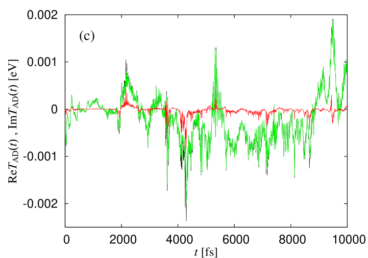
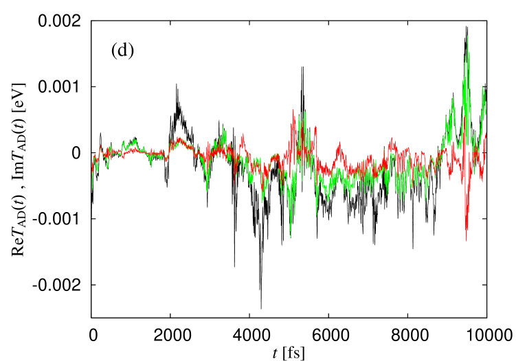
Figure 4: $\mathrm{Re}T_{\mathrm{AD}}(t)$ (green line), $\mathrm{Im}T_{\mathrm{AD}}(t)$ (red line) with level broadening, and $T_{\mathrm{AD}}^{\mathrm{pert}}(t)$ (black line) without level broadening for the CS from the LUMO of anthracene to the LUMO of TCNE in PhCN. The level broadening is chosen as (a) $\Gamma=1$ eV, (b) $\Gamma=0.1$ eV, (c) $\Gamma=0.01$ eV, (d) $\Gamma=0.001$ eV.

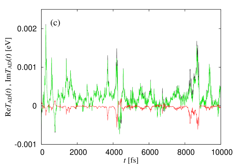
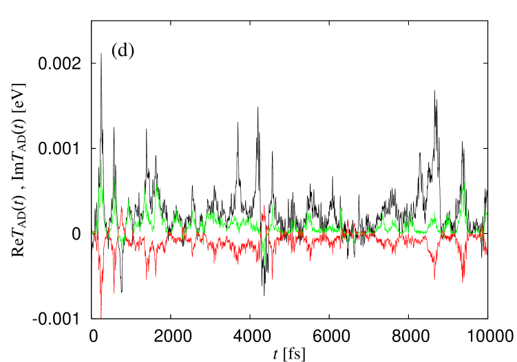
Figure 5: $\mathrm{Re}T_{\mathrm{AD}}(t)$ (green line), $\mathrm{Im}T_{\mathrm{AD}}(t)$ (red line) with level broadening, and $T_{\mathrm{AD}}^{\mathrm{pert}}(t)$ (black line) without level broadening for the CR from the LUMO of TCNE to the HOMO of naphthalene in PhCN. The level broadening is chosen as (a) $\Gamma=1$ eV, (b) $\Gamma=0.1$ eV, (c) $\Gamma=0.01$ eV, (d) $\Gamma=0.001$ eV.

The self-energy is a non-Hermitian matrix. The anti-Hermitian component of the self-energy is responsible for the broadening of the energy levels, while the Hermitian component can conceptually be viewed as a correction to the system Hamiltonian $\hat{H}_{\mathrm{S}}$. For simplicity we ignore the mixing of the states of the relevant system by the coupling to the surroundings. In this case the self-energy becomes diagonal in the basis of eigenstates of the system Hamiltonian $\hat{H}_{\mathrm{S}}$. Furthermore, the energy dependence is disregarded, and all the diagonal elements are set equal. Consequently, the real part of the self-energy vanishes, and the reservoir effect is characterized by a single level broadening parameter, which we denote $\Gamma$. Due to the level broadening term, $T_{\mathrm{AD}}$ is complex, and the time correlation function $C_{\mathrm{A}}^{\mathrm{cl}}(t)$ is decomposed into two autocorrelation functions of the real and imaginary parts of $T_{\mathrm{AD}}$ as in Eq. (III). Figures 4 and 5 show the consequences of including the level broadening.

Figure 4 summarizes a representative set of simulations of $\mathrm{Re}T_{\mathrm{AD}}(t)$ (green line) and $\mathrm{Im}T_{\mathrm{AD}}(t)$ (red line) for the CS from the LUMO of anthracene to the LUMO of TCNE. For (a), (b), (c), and (d), the level broadening is chosen as (a) $\Gamma=1$ eV, (b) $\Gamma=0.1$ eV, (c) $\Gamma=0.01$ eV, (d) $\Gamma=0.001$ eV. For comparison $T_{\mathrm{AD}}^{\mathrm{pert}}(t)$ of Fig. 1 is superimposed on each graph (black line).

Reasonably good agreement of the full $T$-matrix result with $T_{\mathrm{AD}}^{\mathrm{pert}}(t)$ is obtained by choosing $\Gamma$ to be $\simeq 0.01-0.1$ eV (Figs. 4(b) and (c)), where the contribution of $\mathrm{Im}T_{\mathrm{AD}}(t)$ is negligibly small compared to that of $\mathrm{Re}T_{\mathrm{AD}}(t)$. When $\Gamma$ is set larger or smaller (Figs. 4(a) and (d)), the contribution of $\mathrm{Im}T_{\mathrm{AD}}(t)$ becomes significant, and the full $T$-matrix result apparently deviates from $T_{\mathrm{AD}}^{\mathrm{pert}}(t)$.

We get similar behavior patterns for the CR from the LUMO of TCNE to the HOMO of naphthalene as shown in Fig. 5, though the deviation at small level broadening becomes smaller due to the higher energy separation between the D and B LUMO levels.

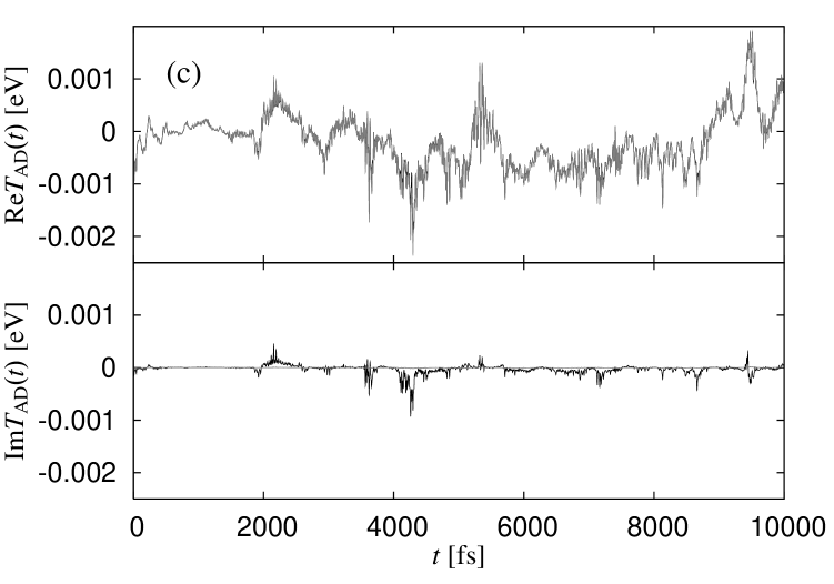
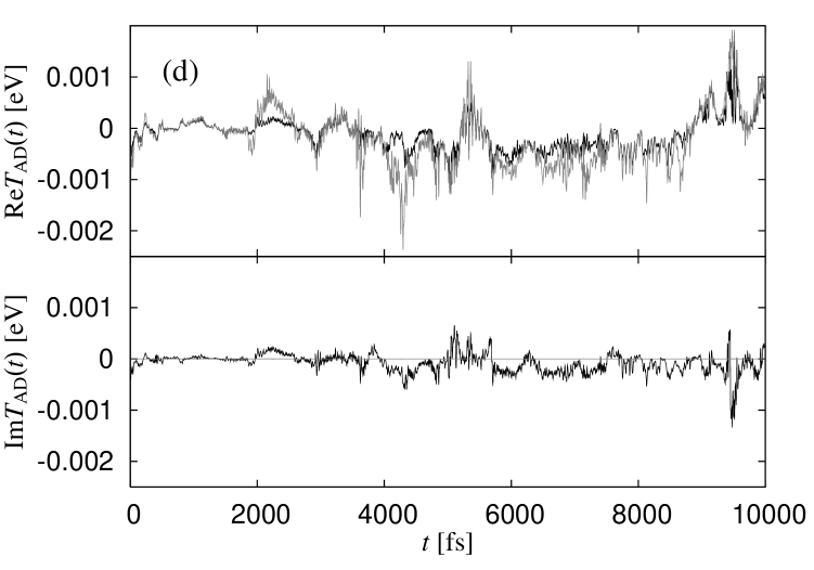
Figure 6: $\mathrm{Re}T_{\mathrm{AD}}(t)$ and $\mathrm{Im}T_{\mathrm{AD}}(t)$ with level broadening for the CS from the LUMO of anthracene to the LUMO of TCNE in PhCN. The gray line is the second-order perturbation result, and the black line is the full $T$-matrix result. The level broadening is chosen as (a) $\Gamma=1$ eV, (b) $\Gamma=0.1$ eV, (c) $\Gamma=0.01$ eV, (d) $\Gamma=0.001$ eV.

To analyze the origin of the deviation, we compare the full $T$-matrix and the second-order perturbation results for the CS from the LUMO of anthracene to the LUMO of TCNE, including the level broadening in both calculations, in Fig. 6. The full $T$-matrix includes all possible intermediate multiple-scattering processes and thus the D and A orbitals as intermediate states. On the other hand, the second-order perturbation theory exclude them from the intermediate processes. Consequently, the deviation of the full $T$-matrix result from the second-order perturbation result arises due to the participation of the D and A orbitals, particularly the initial electronic state, in the intermediate processes. In Fig. 6, the gray line is the second-order perturbation result, and the black line is the full $T$-matrix result. Figures 6(c) and (d) clearly show that the deviation becomes apparent when we use a smaller broadening parameter. In Figs. 6(a) and (b) both results are almost identical. Similar results can be obtained for the CR from the LUMO of TCNE to the HOMO of naphthalene (data not shown). In conclusion, the deviation between the full $T$-matrix and the second-order perturbation results at small level broadening can be attributed to an underestimate of the level broadening for the initial electronic state, while the deviation at large level broadening can be attributed to an overestimate of the level broadening for the B states. In the latter case significant differences do not appear between the full $T$-matrix and the second-order perturbation calculations including the level broadening because they both involve the B states for which the large level broadening causes the error.

VI Resonant tunneling regime

We now turn to the resonant tunneling regime. In the previous section we have considered the CS from the LUMO of anthracene to the LUMO of TCNE and the CR from the LUMO of TCNE to the HOMO of naphthalene in PhCN solvent. Here the LUMO energies of anthracene and TCNE and the HOMO energy of naphthalene lie deep inside the solvent HOMO-LUMO gap. To realize the resonant tunneling regime, we consider the CS from the LUMO of naphthalene to the LUMO of TCNE in the same solvent, whereby the LUMO energy of D is shifted into resonance with the solvent LUMO. In the previous section we have seen that for $\Gamma\simeq 0.01-0.1$ eV we get the best results. This estimation of the level broadening may also be used for the D, A, and B states here, considering the similarities in chemical structure, namely, cyano groups in TCNE and PhCN, and aromatic rings in anthracene, naphthalene, and PhCN. These similarities suggest similar interactions with the reservoir, and thus we expect a similar level broadening.

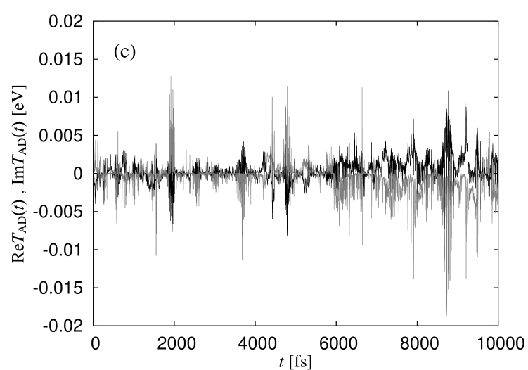
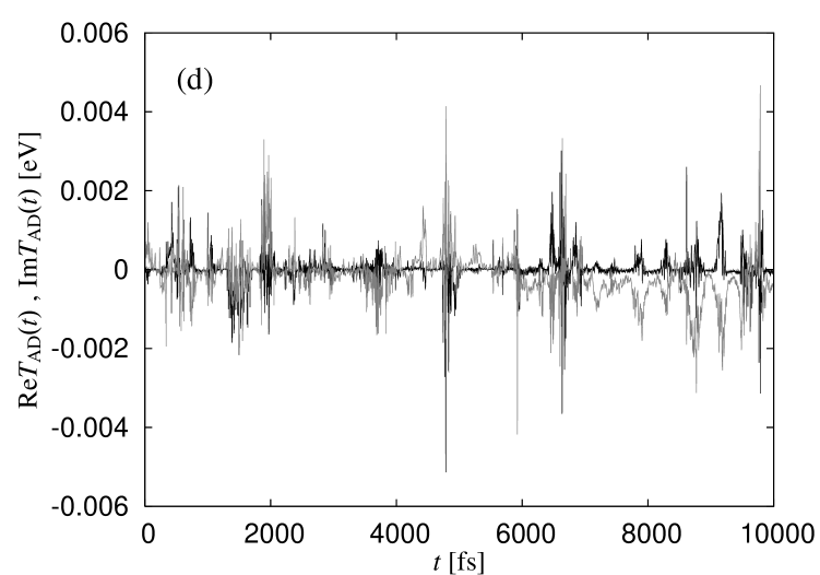
Figure 7: $\mathrm{Re}T_{\mathrm{AD}}(t)$ (black line) and $\mathrm{Im}T_{\mathrm{AD}}(t)$ (gray line) with level broadening for the CS from the LUMO of naphthalene to the LUMO of TCNE in PhCN. The level broadening is chosen as (a) $\Gamma=1$ eV, (b) $\Gamma=0.1$ eV, (c) $\Gamma=0.01$ eV, (d) $\Gamma=0.001$ eV.

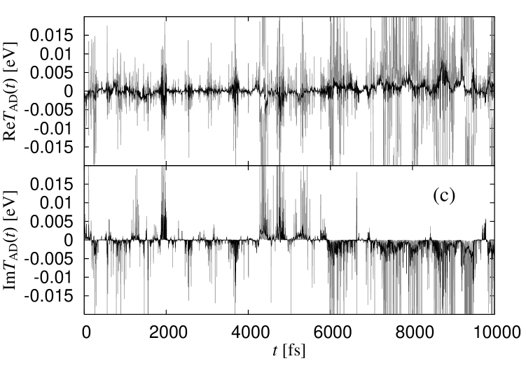
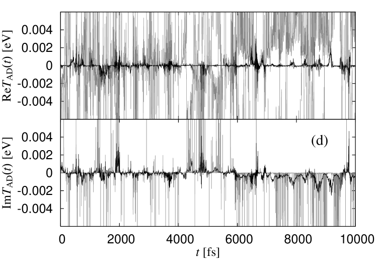
Figure 8: $\mathrm{Re}T_{\mathrm{AD}}(t)$ and $\mathrm{Im}T_{\mathrm{AD}}(t)$ with level broadening for the CS from the LUMO of naphthalene to the LUMO of TCNE in PhCN. The gray line is the second-order perturbation result, and the black line is the full $T$-matrix result. The level broadening is chosen as (a) $\Gamma=1$ eV, (b) $\Gamma=0.1$ eV, (c) $\Gamma=0.01$ eV, (d) $\Gamma=0.001$ eV.

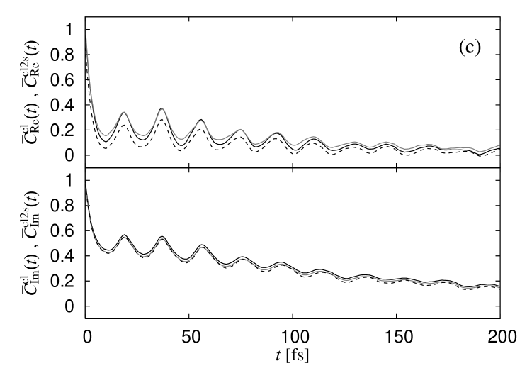
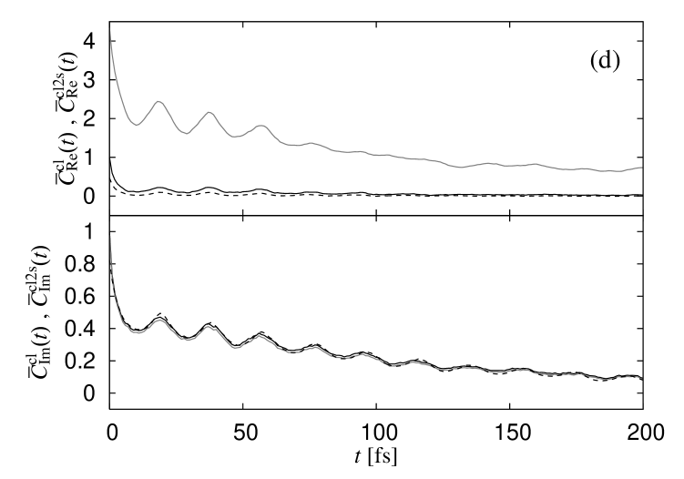
Figure 9: $\bar{C}_{\mathrm{Re}}^{\mathrm{cl}}(t)$ (black solid line), $\bar{C}_{\mathrm{Re}}^{\mathrm{cl2s}}(t)$ (gray solid line), $\bar{C}_{\mathrm{Im}}^{\mathrm{cl}}(t)$ (black solid line), and $\bar{C}_{\mathrm{Im}}^{\mathrm{cl2s}}(t)$ (gray solid line) for the CS from the LUMO of naphthalene to the LUMO of TCNE in PhCN. The black dashed lines are the approximation results for $\bar{C}_{\mathrm{Re}}^{\mathrm{cl2s}}(t)$ and $\bar{C}_{\mathrm{Im}}^{\mathrm{cl2s}}(t)$ using Eqs. (VI) and (VI). The level broadening is chosen as (a) $\Gamma=1$ eV, (b) $\Gamma=0.1$ eV, (c) $\Gamma=0.01$ eV, (d) $\Gamma=0.001$ eV.

Figure 7 shows the patterns of $\mathrm{Re}T_{\mathrm{AD}}(t)$ (black line) and $\mathrm{Im}T_{\mathrm{AD}}(t)$ (gray line) with the level broadening parameter chosen as above in (a), (b), (c), and (d), respectively. From this we can see that the $T$-matrix includes a substantial contribution from the imaginary part. In Fig. 8 the same data (black line) are shown in comparison with the second-order perturbation results with the level broadening (gray line). This indicates that for the small level broadening the second-order perturbation theory fails badly in the resonant tunneling regime. In the following, we consider only the full $T$-matrix. The black solid lines in Fig. 9 show the results for the autocorrelation functions $C_{\mathrm{Re}}^{\mathrm{cl}}(t)$ and $C_{\mathrm{Im}}^{\mathrm{cl}}(t)$, normalized to their initial values. We denote the normalized autocorrelation functions by $\bar{C}_{\mathrm{Re}}^{\mathrm{cl}}(t)=C_{\mathrm{Re}}^{\mathrm{cl}}(t)/C_{\mathrm{Re}}^{\mathrm{cl}}(0)$ and $\bar{C}_{\mathrm{Im}}^{\mathrm{cl}}(t)=C_{\mathrm{Im}}^{\mathrm{cl}}(t)/C_{\mathrm{Im}}^{\mathrm{cl}}(0)$. The level broadening parameter in (a)$-$(d) is chosen as above. For (b), (c), and (d), $\bar{C}_{\mathrm{Re}}^{\mathrm{cl}}(t)$ exhibits very fast initial decay and subsequent periodic damping with a period of approximately $20$ fs. In all cases, the oscillation frequencies are almost equal, while the amplitudes of $\bar{C}_{\mathrm{Re}}^{\mathrm{cl}}(t)$ are larger than those of $\bar{C}_{\mathrm{Im}}^{\mathrm{cl}}(t)$. This feature can be understood by analyzing the dominant contributions to $\bar{C}_{\mathrm{Re}}^{\mathrm{cl}}(t)$ and $\bar{C}_{\mathrm{Im}}^{\mathrm{cl}}(t)$. The gray solid lines in Fig. 9 show that for $\bar{C}_{\mathrm{Re}}^{\mathrm{cl}}(t)$ and $\bar{C}_{\mathrm{Im}}^{\mathrm{cl}}(t)$ in (b) and (c) and $\bar{C}_{\mathrm{Im}}^{\mathrm{cl}}(t)$ in (d) the dominant contribution comes from the two adjacent eigenstates of the system Hamiltonian $\hat{H}_{\mathrm{S}}$, which are closest to the LUMO of D (naphthalene), namely the initial electronic state $|\phi_{i}\rangle$, and the LUMO of B (PhCN solvent). The deviations in (a) can be explained by the large contributions from the other eigenstates due to the large level broadening. On the other hand, the deviation from $\bar{C}_{\mathrm{Re}}^{\mathrm{cl}}(t)$ in (d) is more subtle. We will return to this issue later on.

We denote the two adjacent eigenstates by $|\psi_{+}\rangle$ and $|\psi_{-}\rangle$ with the higher eigenenergy $E_{+}$ and the lower eigenenergy $E_{-}$, respectively, their contribution to $T_{\mathrm{AD}}(t)$ by $T_{\mathrm{AD}}^{\mathrm{2s}}(t)$, and the contributions to $\bar{C}_{\mathrm{Re}}^{\mathrm{cl}}(t)$ and $\bar{C}_{\mathrm{Im}}^{\mathrm{cl}}(t)$ by $\bar{C}_{\mathrm{Re}}^{\mathrm{cl2s}}(t)$ and $\bar{C}_{\mathrm{Im}}^{\mathrm{cl2s}}(t)$, respectively. The two states $|\psi_{+}\rangle$ and $|\psi_{-}\rangle$ alternately fluctuate back and forth between the LUMOs of D and B, which are nearly degenerate. To demonstrate this more clearly, we consider a two-state system whose Hamiltonian is written as a sum $\hat{H}_{\mathrm{S}}=\hat{H}_{0}^{\mathrm{2s}}+\hat{V}$. Here we assume that the eigenfunctions of $\hat{H}_{0}^{\mathrm{2s}}$ are given by the initial electronic state $|\phi_{i}\rangle$ and the solvent LUMO, denoted by $|\phi_{\mathrm{B}}\rangle$, with the corresponding eigenvalues $E_{i}$ and $\epsilon_{\mathrm{B}}$, respectively. These states are coupled by the perturbation $\hat{V}$. For simplicity we assume that the two-state system is unaffected by the coupling between the B and A orbitals $|\phi_{\mathrm{B}}\rangle$ and $|\phi_{\mathrm{A}}\rangle$, although the perturbation $\hat{V}$ includes its contribution. In this case, in the basis of the functions $|\phi_{i}\rangle$ and $|\phi_{\mathrm{B}}\rangle$, $\hat{H}_{\mathrm{S}}$ is represented by the matrix

$$\hat{H}_{\mathrm{S}}=\begin{pmatrix}E_{i}&V\,e^{-i\eta}\\ V\,e^{i\eta}&\epsilon_{\mathrm{B}}\end{pmatrix},$$ (82)

where we have denoted $Ve^{i\eta}=\langle\phi_{\mathrm{B}}|\hat{V}|\phi_{i}\rangle$ with $V$ taken real and positive and the phase factor $e^{i\eta}$. The eigenstates and eigenvalues of the Hamiltonian $\hat{H}_{\mathrm{S}}$ are denoted $|\tilde{\psi}_{+}\rangle$ and $|\tilde{\psi}_{-}\rangle$, and $\tilde{E}_{+}$ and $\tilde{E}_{-}$, respectively. The eigenvalues are given by

$$\tilde{E}_{\pm}=\frac{E_{i}+\epsilon_{\mathrm{B}}\pm\sqrt{(E_{i}-\epsilon_{\mathrm{B}})^{2}+4V^{2}}}{2}.$$ (83)

Thus, $|\tilde{\psi}_{+}\rangle$ remains above the initial electronic state and the solvent LUMO while $|\tilde{\psi}_{-}\rangle$ remains below them. The eigenstates are expressed by

$$|\tilde{\psi}_{+}\rangle=\cos\theta\,e^{-i\eta/2}|\phi_{i}\rangle+\sin\theta\,e^{i\eta/2}|\phi_{\mathrm{B}}\rangle,$$ (84)

$$|\tilde{\psi}_{-}\rangle=-\sin\theta\,e^{-i\eta/2}|\phi_{i}\rangle+\cos\theta\,e^{i\eta/2}|\phi_{\mathrm{B}}\rangle,$$ (85)

where

$$\sin\theta=\frac{X}{(1+X^{2})^{1/2}},$$ (86)

$$\cos\theta=\frac{1}{(1+X^{2})^{1/2}},$$ (87)

$$X\equiv\frac{\tilde{E}_{+}-E_{i}}{V}=\frac{V}{\tilde{E}_{+}-\epsilon_{\mathrm{B}}}=\frac{V}{E_{i}-\tilde{E}_{-}}.$$ (88)

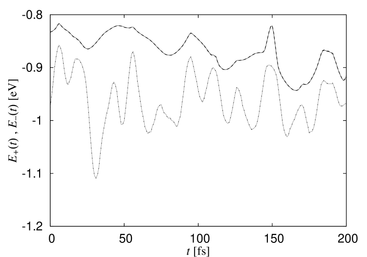
Figure 10: $\tilde{E}_{+}(t)$ (dark gray solid line) in comparison with $E_{+}(t)$ (black dashed line), and $\tilde{E}_{-}(t)$ (gray solid line) in comparison with $E_{-}(t)$ (black dotted line).

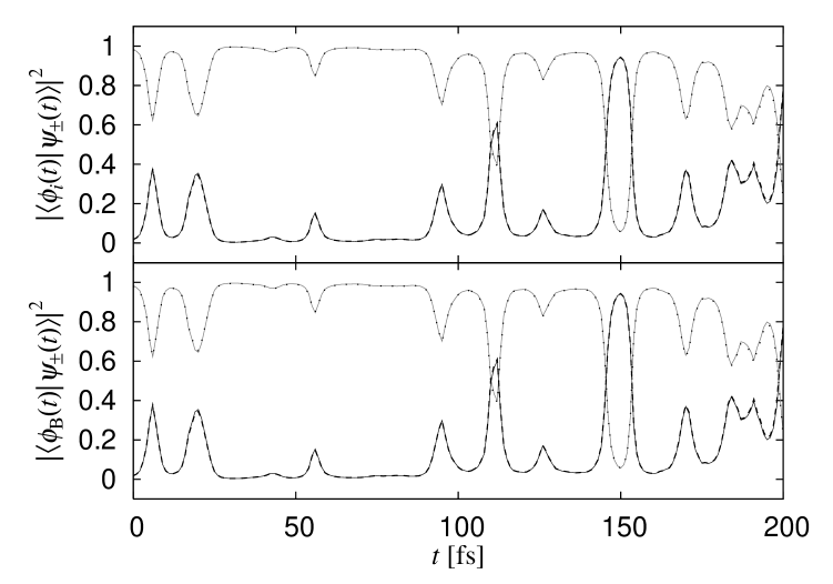
Figure 11: Time dependence of $\sin^{2}\theta$ (dark gray solid line) in comparison with $|\langle\phi_{i}|\psi_{-}\rangle|^{2}$ (black dashed line) and $|\langle\phi_{\mathrm{B}}|\psi_{+}\rangle|^{2}$ (black dashed line), and $\cos^{2}\theta$ (gray solid line) in comparison with $|\langle\phi_{i}|\psi_{+}\rangle|^{2}$ (black dotted line) and $|\langle\phi_{\mathrm{B}}|\psi_{-}\rangle|^{2}$ (black dotted line).

Here $V$ and the eigenstates and eigenvalues of $\hat{H}_{0}^{\mathrm{2s}}$ and $\hat{H}_{\mathrm{S}}$ depend on time via the solvent nuclear coordinates. Figure 10 shows that $\tilde{E}_{+}$ (dark gray solid line) and $\tilde{E}_{-}$ (gray solid line) are very good approximations to the exact eigenenergies $E_{+}$ (black dashed line) and $E_{-}$ (black dotted line), respectively, and Fig. 11 shows that $\sin^{2}\theta$ (dark gray solid line) and $\cos^{2}\theta$ (gray solid line) reproduce the population exchange of $|\phi_{i}\rangle$ and $|\phi_{\mathrm{B}}\rangle$ between the exact eigenstates $|\psi_{+}\rangle$ and $|\psi_{-}\rangle$, described by $|\langle\phi_{i}|\psi_{-}\rangle|^{2}$ (black dashed line) and $|\langle\phi_{i}|\psi_{+}\rangle|^{2}$ (black dotted line) or $|\langle\phi_{\mathrm{B}}|\psi_{+}\rangle|^{2}$ (black dashed line) and $|\langle\phi_{\mathrm{B}}|\psi_{-}\rangle|^{2}$ (black dotted line). These results allow us to approximate $T_{\mathrm{AD}}^{\mathrm{2s}}$ by

$$T_{\mathrm{AD}}^{\mathrm{2s}}\approx\, \langle\phi_{\mathrm{A}}|\hat{V}|\tilde{\psi}_{+}\rangle\frac{1}{E_{i}-\tilde{E}_{+}+i\Gamma/2}\langle\tilde{\psi}_{+}|\hat{V}|\phi_{\mathrm{D}}\rangle$$

$$+\langle\phi_{\mathrm{A}}|\hat{V}|\tilde{\psi}_{-}\rangle\frac{1}{E_{i}-\tilde{E}_{-}+i\Gamma/2}\langle\tilde{\psi}_{-}|\hat{V}|\phi_{\mathrm{D}}\rangle.$$ (89)

Since by definition $\langle\phi_{i}|\hat{V}|\phi_{\mathrm{D}}\rangle=0$, we have

$$T_{\mathrm{AD}}^{\mathrm{2s}}=\mathrm{Re}T_{\mathrm{AD}}^{\mathrm{2s}}+i\mathrm{Im}T_{\mathrm{AD}}^{\mathrm{2s}},$$ (90)

with

$$\mathrm{Re}T_{\mathrm{AD}}^{\mathrm{2s}} \approx\left[\frac{(E_{i}-\tilde{E}_{+})\sin^{2}\theta}{(E_{i}-\tilde{E}_{+})^{2}+(\Gamma/2)^{2}}+\frac{(E_{i}-\tilde{E}_{-})\cos^{2}\theta}{(E_{i}-\tilde{E}_{-})^{2}+(\Gamma/2)^{2}}\right]\langle\phi_{\mathrm{A}}|\hat{V}|\phi_{\mathrm{B}}\rangle\langle\phi_{\mathrm{B}}|\hat{V}|\phi_{\mathrm{D}}\rangle$$

$$\equiv R_{+}+R_{-},$$ (91)

and with

$$\mathrm{Im}T_{\mathrm{AD}}^{\mathrm{2s}} \approx-\left[\frac{(\Gamma/2)\sin^{2}\theta}{(E_{i}-\tilde{E}_{+})^{2}+(\Gamma/2)^{2}}+\frac{(\Gamma/2)\cos^{2}\theta}{(E_{i}-\tilde{E}_{-})^{2}+(\Gamma/2)^{2}}\right]\langle\phi_{\mathrm{A}}|\hat{V}|\phi_{\mathrm{B}}\rangle\langle\phi_{\mathrm{B}}|\hat{V}|\phi_{\mathrm{D}}\rangle$$

$$\equiv I_{+}+I_{-}.$$ (92)

Here, $R_{+}$ and $R_{-}$ denote the contributions of the states $|\tilde{\psi}_{+}\rangle$ and $|\tilde{\psi}_{-}\rangle$, respectively, to the real part $\mathrm{Re}T_{\mathrm{AD}}^{\mathrm{2s}}$, and $I_{+}$ and $I_{-}$ denote the contributions of the states $|\tilde{\psi}_{+}\rangle$ and $|\tilde{\psi}_{-}\rangle$, respectively, to the imaginary part $\mathrm{Im}T_{\mathrm{AD}}^{\mathrm{2s}}$. Since $\tilde{E}_{+}>E_{i}>\tilde{E}_{-}$, $R_{+}$ and $R_{-}$ have opposite signs while $I_{+}$ and $I_{-}$ have the same sign. The black dashed lines in Fig. 9 show this approximation results for $\bar{C}_{\mathrm{Re}}^{\mathrm{cl2s}}(t)$ and $\bar{C}_{\mathrm{Im}}^{\mathrm{cl2s}}(t)$. These plots show very good agreement with the exact results (gray solid lines) except for (d). The deviations are exposed due to the small level broadening. According to Eqs. (83), (VI), and (VI), $|\tilde{\psi}_{+}\rangle$ and $|\tilde{\psi}_{-}\rangle$, which are nearly identical to $|\psi_{+}\rangle$ and $|\psi_{-}\rangle$, respectively, contribute to $\mathrm{Re}T_{\mathrm{AD}}^{\mathrm{2s}}$ destructively, while they contribute to $\mathrm{Im}T_{\mathrm{AD}}^{\mathrm{2s}}$ constructively. Thus, $\mathrm{Re}T_{\mathrm{AD}}$ is more influenced by the other states than $\mathrm{Im}T_{\mathrm{AD}}$. This is the reason why the deviation of $\bar{C}_{\mathrm{Re}}^{\mathrm{cl2s}}(t)$ from $\bar{C}_{\mathrm{Re}}^{\mathrm{cl}}(t)$ is much larger than that of $\bar{C}_{\mathrm{Im}}^{\mathrm{cl2s}}(t)$ from $\bar{C}_{\mathrm{Im}}^{\mathrm{cl}}(t)$.

For the small level broadenings $\Gamma\simeq 0.001-0.1$ eV, the timescale for the initial decay of $\bar{C}_{\mathrm{Re}}^{\mathrm{cl}}(t)$ reaches several femtoseconds and thus may be fast enough to introduce significant dynamical corrections to the ET rate expressions. On the other hand, if the level broadening is as large as $1$ eV, the dynamical non-Condon effects will be insignificant. The rapid initial decay of $\bar{C}_{\mathrm{Re}}^{\mathrm{cl}}(t)$ is followed by the periodic behavior with much the same period. The fluctuations of $\mathrm{Re}T_{\mathrm{AD}}$ and $\mathrm{Im}T_{\mathrm{AD}}$ are caused by the solvent motions. From the timescale viewpoint, we infer that the periodic behaviors of the autocorrelation functions are caused by bond stretching vibrations of PhCN. The higher frequency components in the initial decay should be created by the coupling between various vibrational modes.

The ET rate can be calculated using Eq. (73). For $\tilde{C}_{\mathrm{A}}^{\mathrm{cl}}(\epsilon/\hslash)/C_{\mathrm{A}}^{\mathrm{cl}}(0)$ we use the Fourier transforms of $\bar{C}_{\mathrm{Re}}^{\mathrm{cl}}(t)$ and $\bar{C}_{\mathrm{Im}}^{\mathrm{cl}}(t)$ in Fig. 9. Figure 10 shows the energy gap dependence of $k_{\mathrm{A}\leftarrow\mathrm{D}}$ for the level broadening chosen as above in (a), (b), (c), and (d), respectively. The gray solid, black solid, and black dashed lines are the results for the quantum correction factors of Eqs. (68), (69), and (70), respectively. As expected, for the small level broadenings $\Gamma\simeq 0.001-0.1$ eV, the dynamical non-Condon effects cause the substantial enhancement of the ET rate in the activated inverted region. This enhancement becomes larger with decreasing level broadening. It also depends on the quantum correction factor used. The quantum correction factor of Eq. (69) generates larger enhancement than that of Eq. (68). On the other hand, that of Eq. (70) causes extraordinarily large enhancement of the ET rate regardless of the level broadening because this approximation badly overestimates the value of $\tilde{C}_{\mathrm{A}}(\omega)$ for high frequencies.

VII Conclusion

We have investigated the significance of the dynamical non-Condon effect on the ET rate in the coherent resonant tunneling regime. The time-dependent Fermi’s golden rule expression for the ET rate has been generalized to deal with the resonance in the $T$-matrix framework. The dynamical effect is thereby expressed in terms of the time correlation function of the non-Hermitian $T$-matrix. This time correlation function can be separated into the autocorrelation and the cross-correlation part. The former satisfies detailed balance, whereas the latter does not satisfy it. When the shortest timescale for the change of the time correlation function is comparable to the decay time of the time-dependent Franck-Condon factor, the dynamical non-Condon effects become significant.

In the semiclassical approximation the Fourier transform of the quantum time correlation function is replaced by the classical time correlation function multiplied by the quantum correction factor. In this case the cross-correlation part is disregarded. The classical time correlation function has been evaluated using the combined MD/QC simulations. As an example of the resonant tunneling we have considered the ET from the LUMO of naphthalene to the LUMO of TCNE in PhCN. For simplicity the D and A molecules were held fixed during the simulations. Experimentally, similar situations can be created by linked D-A systems such as C-clamp molecules.

We have introduced the level broadening parameter to include the effect of the surroundings on the relevant system. Disregarding the level broadening leads to unacceptable results even in the deep tunneling regime. The parameter values have been estimated for the CS from the LUMO of anthracene to the LUMO of TCNE and the CR from the LUMO of TCNE to the HOMO of naphthalene in PhCN, which are in the deep tunneling regime. Considering the similarities in chemical structure, we expect a similar level broadening for the above-mentioned resonant tunneling system. By comparing the full $T$-matrix results with the second-order perturbation results, the best parameter values are found to be $\Gamma\simeq 0.01-0.1$ eV. For such level broadenings, the timescale for the initial decay of the time correlation function reaches several femtoseconds, and the ET rate can be significantly enhanced by the dynamical non-Condon effects.

Appendix A

We consider a Hamiltonian written as a sum

$$\hat{H}=\hat{H}_{\mathrm{S}}+\hat{H}_{\mathrm{R}}+\hat{V}_{\mathrm{SR}},$$ (93)

where $\hat{H}_{\mathrm{S}}$ is the Hamiltonian of the relevant system, given by the Fock matrix (8), $\hat{H}_{\mathrm{R}}$ is the Hamiltonian of the surroundings, and $\hat{V}_{\mathrm{SR}}$ is the interaction between them. Let $\{|s\rangle\}$ and $\{|r\rangle\}$ be the orthonormal sets of eigenstates of $\hat{H}_{\mathrm{S}}$ and $\hat{H}_{\mathrm{R}}$, respectively. Then $\hat{H}_{\mathrm{S}}$, $\hat{H}_{\mathrm{R}}$, and $\hat{V}_{\mathrm{SR}}$ may be written in the representation as

$$\hat{H}_{\mathrm{S}}=\sum_{s}E_{s}|s\rangle\langle s|,$$ (94)

$$\hat{H}_{\mathrm{R}}=\sum_{r}E_{r}|r\rangle\langle r|,$$ (95)

$$\hat{V}_{\mathrm{SR}}=\sum_{s,r}(V_{sr}|s\rangle\langle r|+V_{rs}|r\rangle\langle s|),$$ (96)

where we denote $V_{sr}=\langle s|\hat{V}_{\mathrm{SR}}|r\rangle$, etc. The retarded Green’s function of the total Hamiltonian is given by

$$\hat{G}(E)=\frac{1}{E-\hat{H}+i0^{+}}.$$ (97)

We focus on the relevant subspace of the total system and attempt to characterize the effect of the surroundings on the relevant system. The free retarded Green’s function of the relevant system is given by Eq. (13). Then the Dyson equation is expressed as

$$\hat{G}(E)=\hat{G}_{\mathrm{S}}(E)+\hat{G}_{\mathrm{S}}(E)\,\hat{V}_{\mathrm{SR}}\,\hat{G}(E).$$ (98)

Using the resolution of the identity operator

$$\sum_{s}|s\rangle\langle s|+\sum_{r}|r\rangle\langle r|=1$$ (99)

leads to

$$G_{s^{\prime}s}(E)=(G_{\mathrm{S}})_{ss}(E)\,\delta_{s^{\prime},s}+(G_{\mathrm{S}})_{s^{\prime}s^{\prime}}(E)\sum_{r}V_{s^{\prime}r}G_{rs}(E),$$ (100)

$$G_{rs}(E)=(G_{\mathrm{S}})_{rr}(E)\sum_{s^{\prime\prime}}V_{rs^{\prime\prime}}G_{s^{\prime\prime}s}(E),$$ (101)

where $G_{s^{\prime}s}(E)=\langle s^{\prime}|\hat{G}(E)|s\rangle$, $(G_{\mathrm{S}})_{ss}(E)=\langle s|\hat{G}_{\mathrm{S}}(E)|s\rangle$, etc. Inserting Eq. (101) into Eq. (100) it follows that

$$\sum_{s^{\prime\prime}}\left[(E-E_{s^{\prime}}+i0^{+})\delta_{s^{\prime},s^{\prime\prime}}-B_{s^{\prime}s^{\prime\prime}}(E)\right]G_{s^{\prime\prime}s}(E)=\delta_{s^{\prime},s},$$ (102)

where $B_{s^{\prime}s^{\prime\prime}}(E)$ are the self-energy matrix elements given by

$$B_{s^{\prime}s^{\prime\prime}}(E)=\sum_{r}\frac{V_{s^{\prime}r}V_{rs^{\prime\prime}}}{E-E_{r}+i0^{+}}.$$ (103)

This defines the effective reduced Green’s function for the relevant subspace. Note that the self-energy matrix is non-Hermitian due to the infinitesimal term $i0^{+}$. For simplicity we assume that the mixing of the states $|s\rangle$ by the coupling to the reservoir can be disregarded, namely we employ the diagonal approximation to the self-energy matrix. Thereby the self-energy matrix elements read

$$B_{ss^{\prime}}(E)=B_{s}(E)\,\delta_{s,s^{\prime}},$$ (104)

with

$$B_{s}(E)=\sum_{r}\frac{|V_{sr}|^{2}}{E-E_{r}+i0^{+}},$$ (105)

and thus the reduced Green’s function becomes a diagonal matrix, that is,

$$G_{s^{\prime}s}(E)=\frac{1}{(E-E_{s}+i0^{+})-B_{s}(E)}\delta_{s^{\prime},s}.$$ (106)

The imaginary part of the self-energy is equal to the broadening of the density of states in the relevant system, while the real part corresponds to the shifts in the energy levels $E_{s}$.

Furthermore, we assume that the set of states $|r\rangle$ constitutes a continuum of states. In this case the summation over $r$ can be replaced by the integral

$$\sum_{r}\rightarrow\int_{-\infty}^{\infty}dE_{r}\rho_{\mathrm{R}}(E_{r}),$$ (107)

where $\rho_{\mathrm{R}}(E)$ denotes the reservoir density of states. Equation (105) now takes the form

$$B_{s}(E)=\int_{-\infty}^{\infty}dE_{r}\frac{\overline{(|V_{sr}|^{2})_{E_{r}}}\,\rho_{\mathrm{R}}(E_{r})}{E-E_{r}+i0^{+}}=\frac{1}{2\pi}\int_{-\infty}^{\infty}dE_{r}\frac{\Gamma_{s}(E_{r})}{E-E_{r}+i0^{+}},$$ (108)

where $\overline{(|V_{sr}|^{2})_{E}}$ is the average of the squared coupling over all continuum levels $r$ that have energy $E$, defined by $\overline{(|V_{sr}|^{2})_{E}}=\sum_{r}|V_{sr}|^{2}\delta(E-E_{r})/\sum_{r}\delta(E-E_{r})=(\rho_{\mathrm{R}}(E))^{-1}\sum_{r}|V_{sr}|^{2}\delta(E-E_{r})$, and where

$$\Gamma_{s}(E)\equiv 2\pi\,\overline{(|V_{sr}|^{2})_{E}}\,\rho_{\mathrm{R}}(E).$$ (109)

In the simplest case where $\Gamma_{s}(E)$ does not depend on $E$ and $s$, we get

$$B_{s}(E)=\frac{\Gamma}{2\pi}\int_{-\infty}^{\infty}dE_{r}\frac{1}{E-E_{r}+i0^{+}}=-i\frac{\Gamma}{2}.$$ (110)

In this case the effective reduced Green’s function can be expressed in the form

$$\hat{G}(E)=\frac{1}{E-\hat{H}_{\mathrm{S}}+i\Gamma/2}.$$ (111)

Note that the infinitesimal term $i0^{+}$ in Eq. (106) can be disregarded relative to $i\Gamma/2$.

Figure 1: $T_{\mathrm{AD}}^{\mathrm{pert}}(t)$ for (a) the CS from the LUMO of anthracene to the LUMO of TCNE in PhCN, and (b) the CR from the LUMO of TCNE to the HOMO of naphthalene in PhCN.

Figure 2: $\bar{C}_{\mathrm{A}}^{\mathrm{cl}}(t)$ from $T_{\mathrm{AD}}^{\mathrm{pert}}(t)$ for (a) the CS from the LUMO of anthracene to the LUMO of TCNE in PhCN, and (b) the CR from the LUMO of TCNE to the HOMO of naphthalene in PhCN.

Figure 3: $T_{\mathrm{AD}}(t)$ without level broadening for (a) the CS from the LUMO of anthracene to the LUMO of TCNE in PhCN, and (b) the CR from the LUMO of TCNE to the HOMO of naphthalene in PhCN.

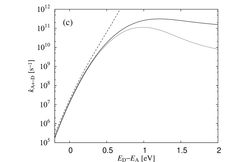
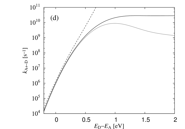
Figure 12: Energy gap dependence of the ET rate. The gray solid, black solid, and black dashed lines are the results for the quantum correction factors of Eqs. (68), (69), and (70), respectively. The level broadening is chosen as (a) $\Gamma=1$ eV, (b) $\Gamma=0.1$ eV, (c) $\Gamma=0.01$ eV, (d) $\Gamma=0.001$ eV.

References

- (1) A. Nitzan, Chemical Dynamics in Condensed Phases, Oxford University Press, Oxford (2006).
- (2) J. Tang, J. Chem. Phys. 98, 6263 (1993).
- (3) I. A. Goychuk, E. G. Petrov, and V. May, J. Chem. Phys. 103, 4937 (1995).
- (4) I. Daizadeh, E. S. Medvedev, and A. A. Stuchebrukhov, Proc. Natl. Acad. Sci. USA 94, 3703 (1997).
- (5) E. S. Medvedev and A. A. Stuchebrukhov, J. Chem. Phys. 107, 3821 (1997).
- (6) M. Bixon and J. Jortner, Russian J. Electrochem. 39, 5 (2003).
- (7) A. Troisi, A. Nitzan, and M. A. Ratner, J. Chem. Phys. 119, 5782 (2003).
- (8) A. Troisi, M. A. Ratner, and M. B. Zimmt, J. Am. Chem. Soc. 126, 2215 (2004).
- (9) S. S. Skourtis, I. A. Balabin, T. Kawatsu, and D. N. Beratan, Proc. Natl. Acad. Sci. USA 102, 3552 (2005).
- (10) H. Nishioka, A. Kimura, T. Yamato, T. Kawatsu, and T. Kakitani, J. Phys. Chem. B 109, 15621 (2005).
- (11) P. Schofield, Phys. Rev. Lett. 4, 239 (1960).
- (12) P. A. Egelstaff, Adv. Phys. 11, 203 (1962).
- (13) B. J. Berne, J. Jortner, and R. Gordon, J. Chem. Phys. 47, 1600 (1967).
- (14) B. J. Berne and G. D. Harp, Adv. Chem. Phys. 17, 63 (1970).
- (15) S.-C. An, C. J. Montrose, and T. A. Litovitz, J. Chem. Phys. 64, 3717 (1976).
- (16) D. W. Oxtoby, Adv. Chem. Phys. 47, 487 (1981).
- (17) P. H. Berens, S. R. White, and K. R. Wilson, J. Chem. Phys. 75, 515 (1981).
- (18) L. Frommhold, Collision-induced Absorption in Gases, Cambridge University Press, Cambridge (1993).
- (19) J. S. Bader and B. J. Berne, J. Chem. Phys. 100, 8359 (1994).
- (20) J. L. Skinner, J. Chem. Phys. 107, 8717 (1997).
- (21) S. A. Egorov and J. L. Skinner, Chem. Phys. Lett. 293, 469 (1998).
- (22) S. A. Egorov, K. F. Everitt, and J. L. Skinner, J. Phys. Chem. A 103, 9494 (1999).
- (23) J. L. Skinner and K. Park, J. Phys. Chem. B 105, 6716 (2001).
- (24) H. Kim and P. J. Rossky, J. Phys. Chem. B 106, 8240 (2002).
- (25) D. M. Lockwood, Y.-K. Cheng, and P. J. Rossky, Chem. Phys. Lett. 345, 159 (2001).
- (26) D. Rehm and A. Weller, Isr. J. Chem. 8, 259 (1970).
- (27) M. Bixon and J. Jortner, Adv. Chem. Phys. 106, 35 (1999).
- (28) M. D. Newton, Adv. Chem. Phys. 106, 303 (1999).
- (29) J. C. Phillips, R. Braun, W. Wang, J. Gumbart, E. Tajkhorshid, E. Villa, C. Chipot, R. D. Skeel, L. Kale, and K. Schulten, J. Comput. Chem. 26, 1781 (2005).
- (30) M. Seeber, M. Cecchini, F. Rao, G. Settanni, and A. Caflisch, Bioinformatics 23, 2625 (2007).
- (31) W. D. Cornell, P. Cieplak, C. I. Bayly, I. R. Gould, K. M. Merz Jr., D. M. Ferguson, D. C. Spellmeyer, T. Fox, J. W. Caldwell, and P. A. Kollman, J. Am. Chem. Soc. 117, 5179 (1995).
- (32) D. A. Case, T. A. Darden, T. E. Cheatham, III, C. L. Simmerling, J. Wang, R. E. Duke, R. Luo, K. M. Merz, D. A. Pearlman, M. Crowley, R. C. Walker, W. Zhang, B. Wang, S. Hayik, A. Roitberg, G. Seabra, K. F. Wong, F. Paesani, X. Wu, S. Brozell, V. Tsui, H. Gohlke, L. Yang, C. Tan, J. Mongan, V. Hornak, G. Cui, P. Beroza, D. H. Mathews, C. Schafmeister, W. S. Ross, and P. A. Kollman (2006), AMBER 9, University of California, San Francisco.
- (33) X. Grabuleda, C. Jaime, P. A. Kollman, J. Comput. Chem. 21, 901 (2000).
- (34) Gaussian 03, Revision C.02, M. J. Frisch, G. W. Trucks, H. B. Schlegel, G. E. Scuseria, M. A. Robb, J. R. Cheeseman, J. A. Montgomery, Jr., T. Vreven, K. N. Kudin, J. C. Burant, J. M. Millam, S. S. Iyengar, J. Tomasi, V. Barone, B. Mennucci, M. Cossi, G. Scalmani, N. Rega, G. A. Petersson, H. Nakatsuji, M. Hada, M. Ehara, K. Toyota, R. Fukuda, J. Hasegawa, M. Ishida, T. Nakajima, Y. Honda, O. Kitao, H. Nakai, M. Klene, X. Li, J. E. Knox, H. P. Hratchian, J. B. Cross, V. Bakken, C. Adamo, J. Jaramillo, R. Gomperts, R. E. Stratmann, O. Yazyev, A. J. Austin, R. Cammi, C. Pomelli, J. W. Ochterski, P. Y. Ayala, K. Morokuma, G. A. Voth, P. Salvador, J. J. Dannenberg, V. G. Zakrzewski, S. Dapprich, A. D. Daniels, M. C. Strain, O. Farkas, D. K. Malick, A. D. Rabuck, K. Raghavachari, J. B. Foresman, J. V. Ortiz, Q. Cui, A. G. Baboul, S. Clifford, J. Cioslowski, B. B. Stefanov, G. Liu, A. Liashenko, P. Piskorz, I. Komaromi, R. L. Martin, D. J. Fox, T. Keith, M. A. Al-Laham, C. Y. Peng, A. Nanayakkara, M. Challacombe, P. M. W. Gill, B. Johnson, W. Chen, M. W. Wong, C. Gonzalez, and J. A. Pople, Gaussian, Inc., Wallingford CT, 2004.
- (35) J. J. P. Stewart, J. Comput. Chem. 10, 209 (1989).
- (36) M. B. Zimmt and D. H. Waldeck, J. Phys. Chem. A 107, 3580 (2003).