A Measurement of the $t\bar{t}$ Cross Section in $p\bar{p}$ Collisions at $\sqrt{s}=1.96$ TeV using Dilepton Events with a Lepton plus Track Selection

Abstract

This paper reports a measurement of the cross section for the pair production of top quarks in $p\bar{p}$ collisions at $\sqrt{s}=1.96$ TeV at the Fermilab Tevatron. The data was collected from the CDF Run II detector in a set of runs with a total integrated luminosity of 1.1 fb^-1. The cross section is measured in the dilepton channel, the subset of $t\bar{t}$ events in which both top quarks decay through $t\to Wb\to\ell\nu b$, where $\ell=e$, $\mu$, or $\tau$. The lepton pair is reconstructed as one identified electron or muon and one isolated track. The use of an isolated track to identify the second lepton increases the $t\bar{t}$ acceptance, particularly for the case in which one $W$ decays as $W\rightarrow\tau\nu$. The purity of the sample may be further improved at the cost of a reduction in the number of signal events, by requiring an identified $b$-jet. We present the results of measurements performed with and without the request of an identified $b$-jet. The former is the first published CDF result for which a $b$-jet requirement is added to the dilepton selection. In the CDF data there are 129 pretag lepton + track candidate events, of which 69 are tagged. With the tagging information, the sample is divided into tagged and untagged sub-samples, and a combined cross section is calculated by maximizing a likelihood. The result is $\sigma_{t\bar{t}}=9.6\pm 1.2(\textrm{stat.})_{-0.5}^{+0.6}(\textrm{sys.})\pm 0.6(\textrm{lum.})$ pb, assuming a branching ratio of $BR(W\rightarrow\ell\nu)=10.8$ % and a top mass of $m_{t}=175\ \mathrm{Ge\kern-1.00006ptV}/c^{2}$.

I Introduction

Top quark data collected at the Tevatron have been an active testing ground for the validity of the standard model since the discovery of the top quark in 1995 during Run I Abe et al. (1995); Abachi et al. (1995). The definitive observation at both the CDF and DØ experiments used data where one or both $W$’s from the top decays $t\to W^{+}b$ and $\bar{t}\to W^{-}\bar{b}$ decay in turn to a charged lepton and neutrino.

This paper focuses on the dilepton channel, in which both $W$’s decay to leptons. The final state contains two isolated charged leptons with large momentum in the direction transverse to the beamline ($p_{T}$). The two neutrinos also carry large transverse momentum but escape the detector without interacting. Their presence can be inferred by an imbalance in the total reconstructed transverse momentum in the detector, referred to as the missing transverse energy (${\not\!\!E_{T}}$) because it is reconstructed from calorimeter information. Only the momentum transverse to the beam can be used for this because in hadron collisions, the total longitudinal momentum of the system is not known in any one collision, and large longitudinal momentum may also be carried by very forward prongs which escape detection. Combined with the jets produced by the hadronization of the $b$ quarks, the distinctive signature of the charged and neutral leptons allows the $t\bar{t}$ signature to be distinguished from the background.

The top quark is unique because of its large mass ($m_{t}=173.1\pm 0.6\ (\textrm{stat.})\pm 1.1\ (\textrm{sys.})\ \mathrm{Ge\kern-1.00006ptV}/c^{2}$ Tevatron Electroweak Working Group (2009)), which distinguishes it from the other fermions of the standard model and is more akin to the masses of the weak force carriers ($W$ and $Z$) and the expected mass range for the proposed Higgs boson Amsler et al. (2008). In Run II of the Tevatron, at center-of-mass energy of 1.96 TeV, the CDF detector has collected well over ten times the amount of integrated luminosity obtained in Run I. Using these data, the study of the top quark sector continues, motivated by a desire to better understand this unique corner of the standard model and to test for physics beyond what the model is able to describe.

Precise measurements of the cross section are of fundamental interest because the top quark is one of the most recent additions to the array of particles that can be produced in the laboratory. The standard model predicts the production of top quark-antiquark pairs through the strong interaction. The leading order Feynman diagrams are shown in Fig. 1. Approximately 85% of $t\bar{t}$ pairs at the Tevatron are produced through quark-antiquark annihilation, and the remaining 15% through gluon-gluon fusion Cacciari et al. (2004). Because of the interaction scale involved, the cross section can be calculated using perturbative QCD techniques. The pair production cross section has been calculated at next-to-leading order (NLO), with the resummation of the leading logarithmic corrections due to the radiation of soft gluons completed to next-to-leading logarithmic (NLL) order Bonciani et al. (1998); Kidonakis and Vogt (2003). These resummations do not change the calculated cross section by more than a few percent, but improve the stability of the result with respect to the normalization and factorization scales Cacciari et al. (2004). Recent updates to the cross section calculation Cacciari et al. (2008); Kidonakis and Vogt (2008); Moch and Uwer (2008) include newer parton distribution functions (PDFs) sets, with reduced associated uncertainties, and incorporate calculations of next-to-next-to-leading order (NNLO) terms. The predicted cross sections cited here have an accuracy of better than 10%. As the accuracy of measurements improves to a comparable level, meaningful comparison with the theoretical prediction becomes possible.

Figure 1: Leading order diagrams for top quark pair production at the Tevatron.

The measurements in this paper were completed using a reference cross section of $6.7_{-0.9}^{+0.7}$ pb, calculated for a top quark mass of $m_{t}=175$ $\mathrm{Ge\kern-1.00006ptV}/c^{2}$ Cacciari et al. (2004). The newer calculations give similar answers with reduced uncertainties. For example, the similar calculation from Ref. Cacciari et al. (2008) gives $6.6^{+0.3}_{-0.5}$ (scale) ${}^{+0.4}_{-0.3}$ (PDF) pb. Most numbers in this paper which depend on the theoretical calculation of the $t\bar{t}$ production cross section are quoted using the original reference cross section, but in the Results section (Sec. IX) we will compare the measured cross sections to the most recent predictions.

Significant deviation of the measured cross section from the predicted value could indicate the presence of new particles or interactions. Top quark pair production cross section measurements can be sensitive to new physics through the production of a new particle or particles which then decay to top quarks. Examples of this include a new heavy top quark of the type predicted by “little Higgs” theories Schmaltz and Tucker-Smith (2005), which decays to a top quark and a stable, heavy analog to the photon, which escapes the detector, adding extra ${\not\!\!E_{T}}$ to the final state. The resulting signature is similar to top quark decay and would enhance the measured cross section. The production of $t\bar{t}$ pairs through a resonance would also raise the total cross section Hill and Parke (1994); Lillie et al. (2007); Baur and Orr (2007), although current limits on resonance production in the $t\bar{t}$ channel make it unlikely that it would be possible to distinguish the effects of a resonance on the cross section at the Tevatron Aaltonen et al. (2008a, b); Abazov et al. (2008a).

The cross section could also be affected by a process with a final state sufficiently similar to the $t\bar{t}$ signature to pass the event selection. The decay of supersymmetric particles is expected to produce multilepton, multijet signatures with significant missing transverse energy from the lightest supersymmetric particles escaping the detector Nilles (1984); Haber and Kane (1985).

Finally, even in the absence of evidence of new physics at the Tevatron, a solid understanding of the top quark sector and the composition of the multilepton + multijet + ${\not\!\!E_{T}}$ sample will be a prerequisite to the discovery and understanding of new physics processes that may appear at the higher energies accessible at the CERN Large Hadron Collider (LHC). This is particularly important because of the approximately hundredfold increase in the $t\bar{t}$ production cross section at the 14 TeV center-of-mass energy at the LHC relative to the Tevatron Cacciari et al. (2008). For example, the possibility of catching the decay signatures of supersymmetric partner particles with event selection designed for top quark pairs implies the converse, that top quark production will be an important background in searches for supersymmetry. Searches for new physics with top quarks in the final state, motivated by models like those referenced above which have a heavy top partner or resonance, will also rely on thorough understanding of the top signature and associated backgrounds.

In this paper, we measure the $t\bar{t}$ production cross section in the dilepton channel. The final state contains two isolated charged leptons with large transverse momentum, missing transverse energy from the undetected neutrinos, and two jets from the hadronization of the $b$ quarks ($b$-jets). One or more additional jets may also be present, having been produced by initial or final state QCD radiation.

The dilepton channel, because of the dual leptonic $W$ decays, has a smaller branching ratio, about 1/9 if all $\tau$ decays are included, than the channels where one or both $W$’s decay to quarks, which are referred to as the “lepton + jets” and “all-hadronic” channels, respectively. The dilepton channel has the compensating advantage of a good (1:1 or better) signal to background ratio even without the identification of jets as possible $b$ decay products (“tagging”), because so few standard model processes produce two high-$p_{T}$ leptons and ${\not\!\!E_{T}}$. Production of events with a $W$ and jets ($W$ + jets) is a background for the dilepton channel, just as it is for the lepton + jets channel, but it does not overwhelm the $t\bar{t}$ signal in spite of its large cross section, because one of the jets must pass the lepton selection used in this analysis. Such a misreconstructed jet is referred to a “fake” lepton. The dilepton channel also does not suffer from the same large QCD multijet background as does the all-hadronic channel, for similar reasons. The background from Drell-Yan ($p\bar{p}\ \to Z/\gamma^{\star}+X\to\ell\ell+X$) is reduced by the requirement of multiple jets and ${\not\!\!E_{T}}$. We also apply several criteria designed specifically to veto Drell-Yan events, including an increased ${\not\!\!E_{T}}$ threshold when the lepton pair has a reconstructed invariant mass close to the $Z$ resonance. Finally, those events which may produce both real leptons and ${\not\!\!E_{T}}$, such as $WW$, are manageable backgrounds because their cross section times branching ratio is comparable to or smaller than that for dilepton $t\bar{t}$ events after the requirement of two or more jets.

We report on two measurements of the $t\bar{t}$ cross section using the dilepton final state, with and without $b$-jet identification, using data collected between March 2002 and February 2006, corresponding to approximately 1.1 fb^-1 of integrated luminosity, using the upgraded Collider Detector at Fermilab (CDF II). These are updates of the previously published result in which one of leptons is reconstructed simply as an isolated track, while the other must be identified as an electron or muon of opposite sign Acosta et al. (2004). The previous version did not use $b$-jet identification. The isolated track selection increases the acceptance by including most decay channels of $\tau$ leptons, thereby increasing the accessible branching fraction. It also recovers acceptance for electrons or muons that are not within the fiducial region of the calorimetry or muon detectors. We will refer to the selection criteria we use (excluding the $b$-jet identification), and the corresponding sample selected from the data, using the name “lepton + track”.

The previous CDF publication used Run II data corresponding to an integrated luminosity of 200 pb^-1. It included a cross section measurement in the lepton + track channel and a similar measurement where both leptons were fully reconstructed as electrons or muons. The combined result was $7.0^{+2.4}_{-2.1}$ (stat.) ${}^{+1.6}_{-1.1}$ (sys.) $\pm 0.4$ (lum.) pb Acosta et al. (2004). The DØ collaboration has also published a measurement in the dilepton channel using Run II data with an integrated luminosity of about 425 pb^-1. It includes measurements where both leptons were fully reconstructed as well as a measurement employing lepton + track and $b$-jet tagging selection similar to that used in this analysis. Combining the individual measurements, they find $7.4\pm 1.4$ (stat.) $\pm 0.9$ (sys.) $\pm 0.5$ (lum.) pb Abazov et al. (2007a).

This measurement is a substantial update of the analysis in the previous CDF publication. It uses more than five times the amount of integrated luminosity. The calculated backgrounds and associated systematic uncertainties reflect an improved understanding of the background composition in the lepton + track sample, with the overall systematic uncertainty decreasing from about 1.4 pb to about 0.55 pb, i.e., from about 20% to 6% relative to the measured values of the cross section. We also perform the cross section measurement using the same event selection, but with the added requirement that at least one jet in the event is $b$-tagged. This significantly suppresses some otherwise irreducible backgrounds, increasing the purity of the candidate sample. The estimated signal to background ratio, using the theoretical cross section of 6.7 pb, is about 6:1 in the $b$-tagged sample, to be compared to about 1:1 in the pretag sample. Finally, we divide the pretag sample into its tagged and untagged components, in order to combine the results into a single cross section result with smaller uncertainties than the individual measurements.

CDF and DØ have also measured the cross section in other $t\bar{t}$ decay modes. In the lepton + jets mode, CDF has used two different methods to identify $b$-jets. One is based on the probability that a large number of tracks within a jet miss the primary vertex, and finds $\sigma_{t\bar{t}}$ = 8.9 ${}^{+1.0}_{-1.0}$ (stat.) ${}^{+1.1}_{-1.0}$ (sys.) pb in a data sample with an integrated luminosity of 320 pb^-1 Abulencia et al. (2006a). The second measurement uses the same sample, but identifies $b$ jets via a reconstructed secondary vertex significantly displaced from the beamline, using the same algorithm as is used in this paper, resulting in a cross section of 8.7 $\pm$ 0.9 (stat.) ${}^{+1.1}_{-0.9}$ (sys.) pb Abulencia et al. (2006b). The DØ collaboration also has two recent results in the lepton + jets channel, both using a data sample with an integrated luminosity of 0.9 fb^-1. The first is a combined result from an analysis requiring a $b$-tagged jet and an analysis using a kinematic likelihood discriminant, with a result of $\sigma_{t\bar{t}}$ = 7.4 $\pm$ 0.5 (stat.) $\pm$ 0.5 (sys.) $\pm$ 0.5 (lum.) pb Abazov et al. (2008b). The second is a simultaneous fit to the cross section and the relative branching ratio $\mathcal{B}(t\to Wb)/\mathcal{B}(t\to Wq)$, where the $q$ represents any down-type quark, resulting in a measured cross section of 8.2 ${}^{+0.9}_{-0.8}$ (stat.+sys.) $\pm$ 0.5 (lum.) pb Abazov et al. (2008c). In the all-hadronic channel, both CDF and DØ base their measurements on events with six or more jets, at least one of which is $b$-tagged. The CDF collaboration applies a neural-net-based discriminant before counting tags, and measures $\sigma_{t\bar{t}}$ = 8.3 $\pm$ 1.0 (stat.) ${}^{+2.0}_{-1.5}$ (sys.) $\pm$ 0.5 (lum.) pb in data with an integrated luminosity of 1.0 fb^-1 Aaltonen et al. (2007). The DØ collaboration also uses a neural-net discriminant and measures 4.5 ${}_{-1.9}^{+2.0}$ (stat.) ${}_{-1.1}^{+1.4}$ (sys.) $\pm$ 0.3 (lum.) pb with 0.4 fb^-1 Abazov et al. (2007b). All these measurements are quoted at the reference mass of $m_{t}=175\ \mathrm{Ge\kern-1.00006ptV}/c^{2}$, and the uncertainty on the integrated luminosity is included in the systematic uncertainty if it is not written separately.

The cross section is determined by the number of candidate events $N_{\mathrm{obs}}$, the integrated luminosity $\int\mathscr{L}dt$, the acceptance times efficiency for $t\bar{t}$ events $\mathcal{A}\epsilon$, and the calculated number of background events $N_{\mathrm{bkg}}$. The acceptance $\mathcal{A}$ is defined as the fraction of $t\bar{t}$ signal events passing the event selection, and includes the branching ratio of the $W$ boson to a lepton pair of a particular flavor, for which we use the the measured value, 0.1080 $\pm$ 0.0009 Amsler et al. (2008). We calculate the cross sections by maximizing the likelihood of obtaining the observed number of candidate events given the number predicted as a function of the $t\bar{t}$ cross section, $\sigma_{t\bar{t}}$. The number predicted, $N_{\mathrm{pred}}$, is the sum of the signal and background contributions:

$$N_{\mathrm{pred}}=\sigma_{t\bar{t}}\mathcal{A}\epsilon\int\mathscr{L}dt+N_{\mathrm{bkg}}\mathrm{.}$$ (1)

The uncertainties are taken from the cross section points where the logarithm of the likelihood decreases by 0.5, and systematic uncertainties are included as nuisance parameters obeying Gaussian probability distributions. The central value from the likelihood maximization is equal to the one obtained from the familiar formula

$$\sigma_{t\bar{t}}=\frac{N_{\mathrm{obs}}-N_{\mathrm{bkg}}}{\mathcal{A}\epsilon\int\mathscr{L}dt}\mathrm{.}$$ (2)

We choose to use a likelihood because it yields statistical uncertainties correctly reflecting the fact that the number of candidates follows a Poisson probability distribution, and allows extraction of a single cross section from multiple data samples.

The paper is structured as follows: First, we briefly describe relevant features of the CDF II detector (Section II). We give details of the observed and simulated data samples in Section III. The event selection is described in Section IV, and the acceptance for that selection, including corrections, is described in Section V. In Section VI, we discuss the algorithm to tag jets from $b$ quarks and calculate the efficiency for tagging lepton + track $t\bar{t}$ events. The background estimation methods for the pretag and tagged samples are described in Sections VII and VIII, respectively. The resulting cross section measurements, including the combination method and combined result, are presented in Section IX.

II The CDF II Detector

The CDF II detector is described in detail elsewhere Abulencia et al. (2007a); we summarize here the components relevant to our measurements. We use a cylindrical coordinate system where $\theta$ is the polar angle defined with respect to the proton beam, $\varphi$ is the azimuthal angle about the beam axis measured relative to the plane of the accelerator, and the pseudorapidity, $\eta$, is defined as $-\ln\tan(\theta/2)$. Transverse energy is defined as $E_{T}=E\sin\theta$, and transverse momentum ($p_{T}$) is defined similarly.

The interaction region of the detector has a Gaussian width of $\sigma_{z}$ = 29 cm. The circular transverse cross section width is approximately 30 $\mu$m at $z$ = 0 cm, rising to 50 $\mu$m at $z$ = 40 cm.

II.1 Tracking

The charged particle tracking system of the CDF detector is contained in a solenoid magnet that produces a 1.4 T field coaxial with the beams, and measures the curvature of particle tracks in the transverse plane. The innermost device employs silicon microstrip sensors, and is composed of three sub-detectors. A single-sided layer of silicon sensors (L00) is installed directly onto the beryllium vacuum beam pipe, at an average radius of 1.5 cm Hill (2004). It is followed by five concentric layers of double-sided silicon sensors (SVXII), located at radii between 2.5 and 10.6 cm Sill et al. (2000). The intermediate silicon layers (ISL) consist of one double-sided layer at a radius of 22 cm in the central region and two double-sided layers at radii of 20 and 28 cm in the forward regions Affolder et al. (2000). Typical strip pitch in the silicon sensors is 55 - 65 $\mu$m for axial strips, 60 - 75 $\mu$m for small-angle stereo strips (1.2^∘), and 125 - 145 $\mu$m for 90^∘ stereo strips. The axial-position resolution of the SVXII sensors is about 12 $\mu$m. For the ISL sensors, it is about 16 $\mu$m.

Surrounding the silicon sensors is the central outer tracker (COT), a 3.1 m long open-cell cylindrical drift chamber covering radii from 40 to 137 cm Affolder et al. (2004). The COT has 96 measurement layers arrayed in eight alternating axial and $2^{\circ}$ stereo superlayers of 12 wires each. The COT provides coverage for $|\eta|<1$, and the fiducial region of the SVXII-ISL system extends out to $|\eta|\sim 2$. The resolution of the combined tracker for tracks with $\theta=90^{\circ}$ is $\sigma(p_{T})/p_{T}^{2}$ = 0.15 %/GeV.

II.2 Calorimetry

Outside of the tracking systems and the solenoid coil are the electromagnetic and hadronic calorimeters which measure the energy of particles that interact electromagnetically or hadronically, respectively. The central electromagnetic calorimeter (CEM) is a lead-scintillator sampling calorimeter which covers the range $|\eta|\leq 1.1$. The CEM has an energy resolution of $13.5\%/\sqrt{E_{T}}$ for electrons and photons Balka et al. (1988). The electromagnetic calorimeter in the forward regions (the “plug”) is of similar design, covers the region $1.2\leq|\eta|\leq 3.6$, and has an energy resolution of $(16\%/\sqrt{E_{T}})\oplus 1\%$ Albrow et al. (2002).

Crucial to electron and photon identification are the shower maximum detectors, placed at a depth of about six radiation lengths in the electromagnetic calorimeter. The shower maximum detectors allow detailed measurement, in the plane approximately transverse to the incident particle direction, of the shower shape at the expected peak of its development. The precision two-dimensional position measurements are made by orthogonal wire proportional chambers and resistive strips in the central calorimeter, and stereo layers of scintillator in the plug calorimeter Nodulman et al. (1983); Apollinari et al. (1998).

The hadronic calorimeter is an iron-scintillator sampling calorimeter, and is between 4.5 and 7 interaction lengths deep, depending on the pseudorapidity. It surrounds the electromagnetic calorimeter and is divided into three sections: the central section covers $|\eta|\lesssim 0.8$, the forward (plug) section covers $1.2\leq|\eta|\leq 3.6$, and the “wall” section covers the intermediate range.

The entire calorimetry system covers the pseudorapidity range $|\eta|<3.6$. All calorimeters are segmented into projective towers which point at the nominal center of the interaction region.

II.3 Muon Detectors

In the pseudorapidity range $|\eta|\lesssim 0.6$, two sets of planar drift chambers are used to identify muons. The inner layer (the CMU, for “Central Muon”) is located just outside of the central hadron calorimeter towers. The outer layer (the CMP, for “Central Muon Upgrade”) is also instrumented with scintillation counters for trigger and timing information. The CMP has a square profile and lies outside the CMU, behind an additional 60 cm of iron shielding. Muons in the region $0.6<|\eta|<1.0$ are detected with the Central Muon Extension (CMX), a layer of drift chambers between layers of scintillator counters. The geometry of the CMX is that of a pair of truncated cones, opening from the interaction point at the center of the detector. The CDF muon system is described in more detail in Refs. Ascoli et al. (1988) and Dorigo et al. (2001). By convention, muons are named according to the muon detector in which they are reconstructed. A CMUP muon has a track segment (“stub”) in both the CMU and CMP detectors.

II.4 Online Event Selection (Trigger)

The 2.5 MHz nominal bunch crossing-rate of the Tevatron far exceeds the rate at which data can be written to permanent storage (75 Hz). CDF uses a three-level trigger system to select a subset of the events to record Winer (2001); Anikeev et al. (2001). Each successive level of processing reduces the event rate and refines the criteria used for event selection.

The first level, is implemented entirely through custom hardware. It uses information from the calorimeter, the axial layers of the COT, and the muon detectors to quickly reconstruct simple objects. Tracks are built from COT axial hits using a predefined set of patterns, and electron and muon candidates are built from tracks matched to energetic towers in the electromagnetic calorimeter and hit segments in the muon detectors, respectively.

Level 1 accepts events and passes them to the next level of processing, level 2, at a rate of up to 50 kHz. Level 2, also built of custom hardware, performs further reconstruction. In particular, clustering of calorimeter towers is performed, for photon, electron, and jet identification.

Events satisfying level 2 criteria are passed to level 3, where they are directed to one of about 300 dual-processor Linux computers. Level 3 applies the full event reconstruction, using the same software that is used for offline analysis, including the application of preliminary calibration constants. This allows more stringent event selection to be made, improving background rejection while maintaining efficiency for signal. Selected events are written to tape for offline analysis.

II.5 Luminosity Determination

Luminosity is measured at CDF by a pair of conical Cerenkov detectors surrounding the beam pipe, at $3.7<|\eta|<4.7$, on each side of the interaction region. Each detector contains 48 smaller mylar cones filled with isobutane at about 1.5 atmospheres of pressure. Photomultiplier tubes at the large ends of the mylar cones collect Cerenkov light produced by particles emerging from inelastic $p\bar{p}$ scattering. The mean number of interactions per beam crossing is inferred from the number of interactions in which no particles are observed in either of the detectors (the “zero-counting method”). The instantaneous luminosity is calculated from the mean number of interactions, the total inelastic $p\bar{p}$ cross section, and the bunch crossing rate. The uncertainties on the luminosity are from the understanding of the acceptance for the detectors as well as the 4% uncertainty on the value of the total $p\bar{p}$ cross section. The combined uncertainty of 6% contributes to the total uncertainty on the cross section.

III Collision Data and Monte Carlo Samples

We measure the $t\bar{t}$ cross section in the subset of the $p\bar{p}$ collision data which appear to have at least one high-$p_{T}$ lepton, as determined by the trigger system. To quantify the signal acceptance, we use a sample of $t\bar{t}$ events which have been simulated using Monte Carlo algorithms. Numerous other observed and simulated data samples are needed to refine the estimated acceptance and estimate the background in the lepton + track sample. In this section we describe the various samples used in this measurement.

III.1 Data Quality Requirements

Because the lepton + track event selection relies on many detector subsystems for the reconstruction of electrons, muons, tracks, jets, and ${\not\!\!E_{T}}$, as well as the measurement of the luminosity, we use only the CDF data in which all of the relevant parts of the detector – the calorimetry, tracking, shower maximum, muon, and luminosity detectors – are fully operational. For the measurement requiring a $b$-tag, we also require the silicon tracking detector to be functioning because high-precision position measurements are necessary for the reconstruction of a displaced secondary vertex. The integrated luminosity of the data sample including information from the silicon detector is 1000 $\pm$ 60 pb^-1. For the pretag measurement, we include an additional $70$ pb^-1 which has no silicon information but which is otherwise acceptable. For these data, PHX (forward) electrons cannot be reconstructed and some tracking requirements are changed, as will be specified in Section IV.

III.2 Data Samples

We select lepton + track $t\bar{t}$ candidates from events passing the high-$p_{T}$ lepton triggers. There are high-$p_{T}$ central and forward electron triggers, as well as triggers for both the CMUP and CMX regions of the muon detectors. The central electron trigger selects events containing a cluster with transverse energy greater than 18 $\mathrm{Ge\kern-1.00006ptV}$ in the central electromagnetic calorimeter and a matched track with $p_{T}>9\ \mathrm{Ge\kern-1.00006ptV}/c$. Track matching is not available online for forward electrons. To reduce the background trigger rate from jets, the electron candidate $E_{T}$ threshold is raised to 20 $\mathrm{Ge\kern-1.00006ptV}$, and the events are required to have at least 15 $\mathrm{Ge\kern-1.00006ptV}$ of ${\not\!\!E_{T}}$. These requirements maintain efficiency for selecting electrons from $W$ decays, where the mean neutrino $p_{T}$ is above 20 $\mathrm{Ge\kern-1.00006ptV}/c$. Both electron triggers require the ratio of the energy in the hadronic calorimeter to the energy in the electromagnetic calorimeter to be less than 0.125 in order to reject hadronic jets. There are separate triggers for CMUP and CMX muons. Each requires a track with $p_{T}>20\ \mathrm{Ge\kern-1.00006ptV}/c$ to be matched with a muon track segment (“stub”) in the relevant detector(s).

Most of the data samples used in this measurement are derived from the set of events passing the high-$p_{T}$ lepton triggers. This includes the $Z$ events used to study lepton identification and the modeling of jet production by QCD radiation, as well as the $W$ + jets sample used in the calculation of the background from events with a fake lepton and the $Z$ + jets sample used in the calculation of the background from $Z/\gamma^{\star}\rightarrow ee/\mu\mu$ + jets events.

To estimate the background from events with a fake lepton, we need a sample with a large number of jets. We use the events passing a photon trigger with a transverse energy threshold of 25 $\mathrm{Ge\kern-1.00006ptV}$.

III.3 Monte Carlo Samples

To calculate the acceptance of the lepton + track selection for the $t\bar{t}$ signal, we apply the event selection to a sample of simulated $t\bar{t}$ events generated using pythia version 6.216 Sjöstrand et al. (2001) for event generation and parton showering. The leptonic branching fraction for the $W$ boson is set to the measured value of 0.1080 $\pm$ 0.0009 Amsler et al. (2008). For the central value of the cross section, we use a sample generated with a top mass of $m_{t}=175\ \mathrm{Ge\kern-1.00006ptV}/c^{2}$. Identical samples generated at other values of the top quark mass are used to recalculate the cross section at those mass points. We also use a sample of $t\bar{t}$ events generated using herwig version 6.510 Corcella et al. (2001) to check the dependence of the calculated acceptance on the event generator.

To estimate the contribution of backgrounds to the lepton + track sample, we use other Monte Carlo samples, which will be described in the relevant sections. Most of them are generated using pythia, in the same version as the signal. For some studies, we use a $W$ + jets sample with matrix elements calculated by alpgen version $2.10^{\prime}$ Mangano et al. (2003) and pythia used for parton showering.

In the Monte Carlo samples in this paper, we use the cteq5l parton distribution functions to model the momentum distribution of the initial state partons Pumplin et al. (2002). The interactions of particles with the detector are modeled using geant version 3 Brun and Carminati (1993), using the gflash parameterization Grindhammer et al. (1990) for showers in the calorimeter. Details on the implementation and tuning of the CDF detector simulation may be found in Ref. Gerchtein and Paulini (2003).

IV Lepton + Track Event Selection

The lepton + track sample is drawn from the set of events with one or more fully reconstructed electron or muon candidates and at least one isolated track which is distinct from the first lepton and has the opposite sign. We also require candidate events to have significant missing transverse energy (${\not\!\!E_{T}}$), a key discriminant between the $t\bar{t}$ signal and backgrounds, particularly Drell-Yan events where the final state leptons are electrons or muons. The ${\not\!\!E_{T}}$ in such events is generally the result of mismeasurement of the energies of leptons or jets and the resulting distribution falls off rapidly with increasing ${\not\!\!E_{T}}$. For this reason, we make a series of corrections to the ${\not\!\!E_{T}}$ and place restrictions on the final-state kinematics to reduce residual contributions from such events.

The requirement that the isolated track has the opposite charge of the fully reconstructed lepton candidate reduces the contribution from events where, due to a fluctuation of fragmentation and hadronization, a jet has reproduced the signature of a lepton candidate. This requirement is nearly 100% efficient for the signal and all other backgrounds, but only 61% efficient for the background from events with jets producing a lepton-like signature.

Finally, we require events to have two or more jets. The $t\bar{t}$ signal contains two $b$ jets at leading order, while the cross sections of the backgrounds are significantly reduced by requiring two or more jets in the final state.

IV.1 Electron Selection

The electron and muon identification criteria used in this analysis are very similar to those described in Ref. Abulencia et al. (2007a). Electron selection is based on a reconstructed track, energy deposition in the electromagnetic calorimeter, and the quality of the match between the track and the energy signature in the calorimeter. This analysis uses two classes of electrons. Central (“CEM”) electrons, in the range $|\eta|\lesssim 1.1$, have tracks in the central tracker and deposit their energy in the central electromagnetic calorimeter. Forward (“PHX”) electrons are identified in the range $1.2\lesssim|\eta|\lesssim 2.0$, and deposit their energy in the plug electromagnetic calorimeter. Forward electrons have tracks that use information from the silicon tracker, and derive their abbreviated name “PHX” from “Phoenix”, the name of the tracking algorithm Acosta et al. (2005a).

IV.1.1 Calorimeter Requirements

First, the calorimeter cluster of the electron must have $E_{T}>20$ $\mathrm{Ge\kern-1.00006ptV}$, calculated after the electron energy has been corrected for calorimeter nonuniformities and the absolute energy scale. The cluster must also be isolated, in the sense that the total energy in the towers in a cone surrounding the tower containing the candidate electron shower is required to be less than 10% of the candidate electron energy. The cone is defined to include objects within $\Delta R=\sqrt{\Delta\eta^{2}+\Delta\varphi^{2}}<0.4$ around the candidate, but the towers in the electron cluster are excluded. The distribution of energy between the towers in the cluster and the shape of the shower in the shower maximum detector are required to be consistent with expectation as determined, for instance, in test beam and studies of electrons from $W$ and $Z$ decays. Finally, the amount of energy deposited in the hadronic part of the calorimeter must be significantly less than the amount deposited in the electromagnetic part. For central electrons, we require that the energy in the hadronic calorimeter be less than 5.5% of the energy in the electromagnetic calorimeter, with a small energy-dependent correction to allow for the fact that showers from more energetic electrons extend farther into the hadronic calorimeter. For plug electrons, we require that the energy in the hadronic calorimeter be less than 5% of the energy in the electromagnetic calorimeter.

IV.1.2 Track Reconstruction and Requirements

Central electron candidate tracks are three-dimensional helices reconstructed from COT hit information. If there are silicon hits in the path of the track through the silicon tracking system, the hits are added and the track is refitted. This makes the measurement of track parameters more precise, but we do not require silicon hits, to maintain efficiency and allow use of data where the silicon tracking detector was not in use. Candidate tracks must have at least three axial and two stereo segments in the COT, where each segment is a set of at least five of twelve possible hits contained in a single superlayer.

Forward electron candidate tracks are reconstructed in the silicon tracker. The track reconstruction algorithm builds seed track helices from plug calorimeter information, taking a point from the shower maximum cluster centroid and another from the interaction vertex. The curvature is estimated by equating the momentum to the energy in the calorimeter. This yields two track hypotheses, one for each choice of sign. A road-based search algorithm attempts to attach silicon hits to each of the track hypotheses, and helices with attached hits are refit for a more precise measurement of the track parameters. The track fit is considered successful if three or more silicon hits are attached and the fit has a $\chi^{2}$ per degree of freedom less than 10. If there are multiple tracks found for an electron candidate, the one with the best fit quality, as measured using the $\chi^{2}$ per degree of freedom, is taken. For both central and plug electron candidates, we require the track to originate from a point along the beam line that is less than 60 cm from the nominal center of the detector ($|z_{0}|<$ 60 cm).

IV.1.3 Conversion veto

Central electrons may be flagged as having originated from a photon conversion if there is a second track near to the electron track with opposite sign. We do not use central electrons which have been flagged as conversions. There is no explicit conversion veto for forward electrons, but the silicon tracking algorithm suppresses tracks from conversions. The algorithm creates a track hypothesis assuming that the electron track is prompt and has momentum equal to the energy in the calorimeter, but these assumptions are wrong for most conversion electrons. Silicon hits from conversion electron tracks will not generally be close enough to the track hypothesis to be attached, and the track finding fails.

IV.2 Muons

Muon candidates are defined as a track in the COT with $p_{T}>20\ \mathrm{Ge\kern-1.00006ptV}/c$ matched to a track segment in one or more of the muon drift chambers. We require either a stub in both the CMU and CMP detectors, or a stub in the CMX detector, and refer to the resulting muon candidates as CMUP or CMX muons, respectively. Requiring muon signatures in both the CMU and CMP detectors reduces the probability of reconstructing a muon from a hadron that reaches the CMU as a result of a particle shower that is not fully contained in the hadronic calorimeter.

IV.2.1 Calorimeter Signature

The energy deposited in the region of the calorimeter intersected by the candidate muon track is required to be consistent with the expectation for a minimum-ionizing particle. Specifically, there must be no more than 2 $\mathrm{Ge\kern-1.00006ptV}$ in the electromagnetic calorimeter and 6 $\mathrm{Ge\kern-1.00006ptV}$ in the hadronic calorimeter, with a small correction for muons with momentum over 100 $\mathrm{Ge\kern-1.00006ptV}/c$ to allow for the expected rise in ionization. We also require muon candidates to be isolated in the sense that the total sum $E_{T}$ in the calorimeter towers in a cone of $\Delta R<0.4$ around the one intersected by the extrapolated muon track is less than 10% of the muon $p_{T}$.

IV.2.2 Tracking Requirements

Muon candidates use the same tracks and track quality requirements as central electron candidates. We make a few additions to the quality requirements from muons, motivated by backgrounds particular to muons, such as cosmic rays and kaon decays-in-flight. In addition to the COT track and $z_{0}$ requirement, the candidate track must have a small impact parameter ($d_{0}$). The impact parameter is the two-dimensional distance, in the plane transverse to the beam direction, between the beamline and the point of closest approach of the track helix to the beamline. We require that the impact parameter for muon tracks be less than 20 (200) $\mu$m for tracks with (without) attached silicon hits. We also require that the $\chi^{2}$, given the number of degrees of freedom in the track fit (i.e., the number of hits on the track minus the number of fit parameters) is such that the probability to have found a larger $\chi^{2}$ for that track by chance is greater than $10^{-8}$. This in essence requires that the track be well reconstructed. It is similar in spirit to a requirement that the $\chi^{2}$ or $\chi^{2}$ per degree of freedom be less than a specified value, but it removes the dependence of the efficiency for good tracks on the number of degrees of freedom.

IV.2.3 Track-Stub Matching

We check the quality of the spatial match between the COT track and the muon stub(s). The quantity used is the distance between the track stub in the muon detectors and the point at which the extrapolated COT track crosses the front plane of the corresponding detector element. The distance is measured in the plane of the muon detector, transverse to the measurement wires. A CMUP muon track must extrapolate to within 7 cm of the CMU stub and within 5 cm of the CMP stub. For CMX, the maximum allowed displacement is 6 cm.

IV.3 Track Lepton Selection

We use an isolated high-$p_{T}$ track to identify the second lepton in the event. To qualify, the tracks must have $p_{T}>$ 20 $\mathrm{Ge\kern-1.00006ptV}/c$, pass certain quality requirements, and be isolated in $\eta-\varphi$ space from other energetic track activity. The track may be left by either a charged lepton or a charged hadron from the decay of a $\tau$ lepton, but it is in either case indicative of the presence of a lepton. The isolated track, in this role, is also referred to as a “track lepton” because its identification relies entirely on information from the tracking detectors, and also to distinguish it from the fully reconstructed electron and muon candidates. The added acceptance for $t\bar{t}$ signal events where one and sometimes even both $W$’s have decayed to a $\tau$ and $\nu_{\tau}$ is discussed in more detail in Sec. V.

IV.3.1 Track quality

As is the case for muons, it is important for the track to be well-measured, both to reject background and because the track momentum is the only measure of the particle’s energy. The track must have at least 24 hits in the axial layers of the COT and at least 20 hits in the stereo layers and satisfy the same $\chi^{2}$ probability requirement as muons. The requirement of a minimum number of track hits limits the acceptance for track leptons to $|\eta|\lesssim 1.15$, according to the geometry of the COT. There is also a maximum allowed impact parameter, 0.025 cm, but unlike the muon case, the requirement is independent of the presence of silicon hits. We also require silicon hits to be present if they are expected, to reduce the incidence of fake tracks reconstructed from accidental combinations of hits. Specifically, if the track passes through three or more layers of the silicon tracker known to be functional, it must have at least three silicon hits attached.

IV.3.2 Track isolation

Track isolation is crucial to the rejection of backgrounds from jets. We sum the $p_{T}$ of every track with $p_{T}>0.5~{}\mathrm{Ge\kern-1.00006ptV}/c$, including the candidate track, within a cone of $\Delta R<0.4$ around the candidate. The ratio of the candidate track $p_{T}$ to the sum $p_{T}$ in the cone is required to be at least 0.9. To be included in the $p_{T}$ sum, tracks must pass quality requirements similar to, but less stringent than, those for the track lepton. No $\chi^{2}$ probability or impact parameter restrictions are made, and only 20 axial and 16 stereo hits are required.

IV.4 Jet Definition

Jet reconstruction is based on a calorimeter tower clustering cone algorithm with a cone size of $\Delta R=0.4$. Towers corresponding to identified electrons according to the definition above are removed before clustering. The $E_{T}$ values of the jets are corrected for the effects of jet fragmentation, calorimeter non-uniformities and the calorimeter absolute energy scale Bhatti et al. (2006).

We extend the jet definition to facilitate the calculation of the rate for a jet to be reconstructed as an isolated track, and use this jet definition everywhere in the analysis for consistency. The details of the fake lepton background calculation are described in Section VII.1, but the core idea is to ensure that any object which could be identified as a track lepton is included in the jet collection, because that jet collection forms the denominator of the measured probability for an object of hadronic origin to be identified as a lepton.

This requires modification of the jet definition. For each track passing all of the track lepton requirements, but ignoring the isolation requirement, we check whether it is within $\Delta R=0.4$ of the axis of a jet. Here, we consider all jets from the cone algorithm with $E_{T}>10$ $\mathrm{Ge\kern-1.00006ptV}$. If the track is not matched, we add it to the jet collection. If it is matched, we check whether the $p_{T}$ of the track exceeds the corrected $E_{T}$ of the jet. If it does, we substitute the kinematic information of the track for the kinematic information for the jet. If the $p_{T}$ of the track is less than the corrected $E_{T}$ of the jet, we leave the jet kinematic information as is. Inclusion of track information in this manner ensures counting of the products of parton fragmentation where most of the momentum is carried by a single charged particle which does not deposit all of its energy in the hadronic calorimeter. In extreme cases, jet energy corrections will not account for all of the unmeasured energy and the track momentum is the best measure of the parton energy.

The final jet collection thus includes standard jets clustered with a cone size of 0.4, jets with kinematic information from tracks, and unaffiliated tracks. For event selection we count the number of jets with $E_{T}>20$ $\mathrm{Ge\kern-1.00006ptV}$ and $|\eta|<2.0$, excluding those jets within $\Delta R\leq 0.4$ of either the lepton candidate or the isolated track. When making a $W$ + jets selection, such as is used in the fake lepton background estimates for both the pretag and tagged samples, only the fully reconstructed lepton is excluded from the jet counting.

IV.5 Missing Transverse Energy Reconstruction

A transverse momentum imbalance in the detector indicates that particles have exited the detector without interacting. Dilepton $t\bar{t}$ events have two high-$p_{T}$ neutrinos in the final state, leading to a considerable amount of ${\not\!\!E_{T}}$ in signal events. Figure 2 shows the simulated ${\not\!\!E_{T}}$ distributions for the $t\bar{t}$ signal and some of the backgrounds. Comparison of these distributions shows that using a ${\not\!\!E_{T}}$ threshold to select events reduces the contribution from many of the backgrounds considered, particularly Drell-Yan events, but is quite efficient for $t\bar{t}$ events.

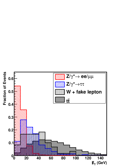
Figure 2: Corrected missing transverse energy from several lepton + track backgrounds, compared to the $t\bar{t}$ signal. The distribution for $WW$ events is similar to the $t\bar{t}$ distribution but slightly softer, and is omitted for legibility. Candidate events are required to have a fully reconstructed lepton and track and two or more jets, but no other event selection is applied. For the cross section measurements, we require events to have $\mbox{${\not\!\!E_{T}}$}>25$ $\mathrm{Ge\kern-1.00006ptV}$. Distributions taken from events generated with pythia and normalized to have unit area.

The missing transverse energy is defined as:

$$\not\!\!\vec{E}_{T}=-\sum_{i}E_{T}^{i}\hat{n}_{i},$$ (3)

where $i$ is an index that runs over all calorimeter towers with $|\eta|<3.6$ and $\hat{n}_{i}$ is a unit vector perpendicular to the beam axis and pointing at the i^th calorimeter tower. The scalar, ${\not\!\!E_{T}}$, is then defined as $\not\!\!E_{T}=|{\not\!\!\vec{E}_{T}}|$.

Some care must be taken with the ${\not\!\!E_{T}}$ calculation, because a transverse momentum imbalance can also be generated by incorrect measurements of objects in the event and the energy resolution of the calorimeter towers themselves. To reduce the inclusion of events where the ${\not\!\!E_{T}}$ is produced by energy mismeasurements, the ${\not\!\!E_{T}}$ is adjusted in those cases where the calorimeter information is not the best measure of an object’s energy.

IV.5.1 Muon Correction

Muons are minimum-ionizing particles and deposit very little energy in the calorimeter. Thus, if the fully reconstructed lepton in the event is a muon (CMUP or CMX), we subtract the transverse components of the muon momentum from the corresponding components of the ${\not\!\!E_{T}}$. No correction is made to the calorimeter energy for the small amount of energy deposited by the muon.

IV.5.2 Track Correction

We also correct for all tracks (excepting the fully reconstructed lepton if it is a muon) pointing at a 3 by 3 block of calorimeter towers where the $E_{T}$ measured is less than 70% of the $p_{T}$ of the track. All tracks with $p_{T}>10\ \mathrm{Ge\kern-1.00006ptV}/c$, $|d_{0}|<250\mu$m, at least 24 (20) hits on the axial (stereo) wires of the COT, and appearing to come from the same interaction vertex ($|\Delta z_{0}|<5$ cm) as the primary lepton, are considered. The 70% threshold excludes normal fluctuations in the energy and momentum resolution, so that we correct only for tracks where the energy deposit measured in the calorimeter is clearly not consistent with the momentum measured in the tracker. This correction accounts for tracks pointing at cracks in the calorimeter, minimum-ionizing particles such as muons, and cases where showers produced by hadronic particles in the calorimeters have unusually low light yields.

IV.5.3 Jet Correction

We also correct the ${\not\!\!E_{T}}$ for the jet energy calibrations by subtracting the difference between the corrected and uncorrected jet energies. By doing this we use the best estimate of the energies of those objects which are identifiable as jets. Jets with corrected $E_{T}>10\ \mathrm{Ge\kern-1.00006ptV}$ and $|\eta|<2.0$ are included, except for objects in the jet collection which are tracks or have had their kinematic information replaced by that of an associated track. These will have already been accounted for in the track correction.

IV.6 Event Selection

IV.6.1 Basic event selection

Having defined our basic analysis objects, we can select events with features typical of $t\bar{t}$ dilepton events. First, there must be at least one fully reconstructed electron or muon with $p_{T}>20\ \mathrm{Ge\kern-1.00006ptV}/c$ in the event. Once a primary lepton is identified, we take as the track lepton the highest $p_{T}$ isolated track with $p_{T}>20\ \mathrm{Ge\kern-1.00006ptV}/c$. To qualify, the track must appear to be from the same interaction vertex as the primary lepton, ($|\Delta z_{0}|<5$ cm). If there is no such isolated track, we try the event selection again with the next fully reconstructed lepton, if another has been identified. The leptons are considered in the following order: central (CEM) electrons, CMUP muons, CMX muons, and finally forward (PHX) electrons. Within a particular lepton type, the leptons are tested in order of descending $E_{T}$ or $p_{T}$. In the CDF data, for a lepton of a particular type to be considered, the trigger corresponding to that category must have fired for that event, and the relevant parts of the detector must be known to be fully functional at the time the event occurred.

After a track lepton is found, we correct the ${\not\!\!E_{T}}$, and require the corrected ${\not\!\!E_{T}}$ to be greater than 25 $\mathrm{Ge\kern-1.00006ptV}$. Each fully reconstructed lepton in an event is considered in turn until the event has passed all of the selection criteria, or has failed them for all leptons.

IV.6.2 $\Delta\varphi$ Requirements

Drell-Yan events may appear to have ${\not\!\!E_{T}}$  in spite of the absence of neutrinos in the final state. If the energy of one lepton or jet is measured incorrectly, false ${\not\!\!E_{T}}$ appears, pointing along or opposite to the direction of that object. For this reason we require that no lepton or jet in the event be pointing directly at the ${\not\!\!E_{T}}$. The requirements for different objects are determined by their respective angular size and potential for mismeasurement. Studies of Drell-Yan events in simulation show that although ${\not\!\!E_{T}}$ may be generated either pointing near or away from a track lepton, most ${\not\!\!E_{T}}$ associated with fully reconstructed leptons or jets is pointing in the same direction as the lepton or jet. These studies also show that it is uncommon for ${\not\!\!E_{T}}$ associated with a jet to exceed 50 $\mathrm{Ge\kern-1.00006ptV}$. Therefore, we veto events where the primary lepton points within $5^{\circ}$ of the ${\not\!\!E_{T}}$ or the track lepton is within $5^{\circ}$ of parallel or anti-parallel to the ${\not\!\!E_{T}}$. Also, all jets in the event must be more than $25^{\circ}$ away from the direction of the ${\not\!\!E_{T}}$, unless the event has ${\not\!\!E_{T}}$ $>50$ $\mathrm{Ge\kern-1.00006ptV}$.

IV.6.3 $Z$ Boson Veto

To further reduce background from Drell-Yan events, the ${\not\!\!E_{T}}$ threshold is raised to 40 $\mathrm{Ge\kern-1.00006ptV}$ if the invariant mass of the lepton + track pair is in the range of the $Z$ boson resonance ($76~{}\mathrm{Ge\kern-1.00006ptV}/c^{2}<M<106~{}\mathrm{Ge\kern-1.00006ptV}/c^{2}$). This requirement is referred to as the “$Z$ veto”.

IV.6.4 Candidate Events

For the cross section measurements we count events with at least two jets with corrected $E_{T}>20\ \mathrm{Ge\kern-1.00006ptV}$ and $|\eta|<2.0$. The jets used for this are the extended collection described in Sec. IV.4, which is based on a calorimeter clustering algorithm with a cone size of $\Delta R<0.4$. Any jets within $\Delta R<0.4$ of either the lepton candidate or the isolated track are excluded from the jet counting. The final requirement is that the fully reconstructed lepton candidate and the track lepton candidate have opposite sign.

Applying this selection to 1.1 fb^-1 of CDF Run II data, we find 129 pretag lepton + track $t\bar{t}$ candidate events with two or more jets.

V $t\bar{t}$ Dilepton Acceptance

We determine the geometric and kinematic acceptance for $t\bar{t}$ dilepton events by applying the lepton + track event selection to the pythia $t\bar{t}$ sample described in Section III. The acceptance is defined as the number of simulated $t\bar{t}$ events passing the selection criteria, divided by the total number of $t\bar{t}$ events in the sample. To be included in the numerator, the event must be identified as a dilepton decay at the generator level, where the $W$’s may decay to any of $e\nu_{e}$, $\mu\nu_{\mu}$, or $\tau\nu_{\tau}$. Other $t\bar{t}$ events passing the event selection are accounted for as background (see Section VII.1). Corrected for discrepancies between observed and simulated data, the acceptance is 0.84 $\pm$ 0.03 %, where the uncertainty includes the systematic uncertainties. In the rest of this section, we discuss the acceptance, the corrections made to it, and the systematic uncertainties on it.

V.1 Contributions to the Acceptance

One of the advantages of identifying the second lepton only as a track is the enhanced acceptance for $\tau$ leptons from $W$ decays. Standard electron and muon selection will accept a fraction of $\tau$ decays, since 35% are through leptonic channels. There will be some inefficiency, because a portion of the momentum of the original $\tau$ will be lost to the two neutrinos produced. On the other hand, if “single-prong” hadronic decays are included, 85% of $\tau$ decays have a single charged track in the final state. About 20% of the total lepton + track acceptance is from events where one or both of the $W$’s decays to a $\tau$ lepton, and 65% of that (13% of the total) is from events where at least one of the $\tau$ leptons decays hadronically. Table 1 shows how the acceptance is distributed among the different lepton types.

	$ee$		$e\mu$		$\mu\mu$		$e\tau$		$\mu\tau$		$\tau\tau$		total
$e$+track	17.4 $\pm$	0.2	29.5 $\pm$	0.3	0.0 $\pm$	0.0	7.6 $\pm$	0.1	2.3 $\pm$	0.1	0.5 $\pm$	0.0	57.4 $\pm$	0.4
$\mu$+track	0.0 $\pm$	0.0	5.9 $\pm$	0.1	15.5 $\pm$	0.2	0.5 $\pm$	0.0	4.8 $\pm$	0.1	0.3 $\pm$	0.0	26.9 $\pm$	0.2
total	17.4 $\pm$	0.2	35.4 $\pm$	0.3	15.5 $\pm$	0.2	8.1 $\pm$	0.1	7.1 $\pm$	0.1	0.8 $\pm$	0.0	84.3 $\pm$	0.5

Table 1: Acceptance for opposite-charge lepton + track events with two or more jets, for each possible pairing of generated charged leptons from the $W$ decays. Numbers have been multiplied by 10000 for legibility. The first row shows the acceptance in the channels where the fully reconstructed lepton is an electron, and the second row shows the acceptance for the fully reconstructed muon channels. The majority of events are accepted as electron plus track because there is more geometric acceptance for electrons, and because the ordering of primary leptons means that events generated as electron-muon events will be preferentially accepted as electron+track. The uncertainties quoted only include the statistical uncertainty.

V.2 Corrections to the Acceptance

To understand the discrepancies in lepton reconstruction between observed and simulated data, we study the performance of the reconstruction in large control samples and derive appropriate corrections. Real and simulated $Z$ boson events are used, because the available samples are large and the reconstruction of the invariant mass peak allows selection of a very pure sample of dilepton events, even with minimal identification requirements placed on the second lepton. We also correct the acceptance for the small inefficiency of the high-$p_{T}$ lepton triggers.

These corrections are also used in some of the background calculations.

V.2.1 Trigger Efficiencies

We measure single lepton trigger efficiencies with a combination of $Z$ data and data taken using an independent trigger. The $Z$ sample is especially useful when the two lepton candidates are found in sections of the detector corresponding to different triggers. Independent triggers designed to share some, but not all, of the requirements of the trigger of interest enable measurement of the efficiency of the omitted requirements.

What we need for the cross section measurements is the probability for a lepton + track candidate to fire one of the high-$p_{T}$ lepton triggers. This probability is higher than the single lepton trigger efficiency since each event has two chances to fire one of the triggers, one for each lepton. On the other hand, the second lepton is not fully reconstructed in our event selection, so the event trigger efficiency is not just a simple combination of single-lepton trigger efficiencies. To determine the per-event trigger efficiency for a particular process and fully reconstructed lepton type, we count the number of events in a simulated sample of that process that have one lepton of that type and the number with two of that type. For events with one fully reconstructed lepton, we use the single-lepton trigger efficiency as the event trigger efficiency. For events with two, we use the probability for at least one of the two leptons to fire the trigger, given by $1-(1-\epsilon)^{2}$ where $\epsilon$ is the single-lepton trigger efficiency. We then take the average of the two per-event efficiencies, weighted by the relative number of events with one and two fully reconstructed leptons. The plug electron trigger also includes a ${\not\!\!E_{T}}$ threshold, so the trigger efficiency we use for those events also depends on the value of the ${\not\!\!E_{T}}$ as it would be calculated for the trigger decision. Note that we include the electron $E_{T}$ and ${\not\!\!E_{T}}$ dependence of the trigger efficiencies where applicable, by convoluting the single-lepton trigger efficiencies with the $E_{T}$ and or ${\not\!\!E_{T}}$ distributions for the class of events in question.

The per-event trigger efficiency is also needed for background estimates that use an acceptance calculated from simulation. For a given lepton type, the per-event efficiencies are very similar across different physics processes, so the $t\bar{t}$ value is used. The one exception is PHX + track $Z/\gamma^{\star}\rightarrow\tau\tau$ events. For those events the typical plug electron $E_{T}$ and ${\not\!\!E_{T}}$ fall in the middle of the turn-on curves for the trigger, and the trigger efficiency, about 66%, is lower than those typical of $t\bar{t}$ and diboson events.

The single-lepton and total per-event trigger efficiencies are given in Table 2.

V.2.2 Fully Reconstructed Electrons and Muons

Identification efficiencies for fully reconstructed leptons are measured in a sample of $Z$ candidates. These candidates consist of one fully reconstructed lepton candidate and one opposite-charge lepton candidate of the same flavor which meets minimal kinematic and identification criteria. The fully reconstructed candidate must pass the corresponding high-$p_{T}$ lepton trigger, and the invariant mass of the lepton candidate pair is required to be close to the central value of the $Z$ resonance peak.

For central (CEM) electrons, the minimally-identified lepton candidate is an electromagnetic cluster fiducial to the central calorimeter with $E_{T}>20\ \mathrm{Ge\kern-1.00006ptV}$ and a matched track with $p_{T}>10\ \mathrm{Ge\kern-1.00006ptV}/c$ and $|z_{0}|<60$ cm. The electron candidate pair must have an invariant mass in the interval $76~{}\mathrm{Ge\kern-1.00006ptV}/c^{2}<M<106~{}\mathrm{Ge\kern-1.00006ptV}/c^{2}$. Electromagnetic clusters fiducial to the forward calorimeter are used to measure the forward (PHX) electron efficiency. No track requirement is made, so the efficiencies measured include the tracking efficiency. The invariant mass window used for this candidate pair is $81~{}\mathrm{Ge\kern-1.00006ptV}/c^{2}<M<101~{}\mathrm{Ge\kern-1.00006ptV}/c^{2}$.

For muons, the total reconstruction efficiency is the product of the efficiency to find a track stub in the muon chambers and the efficiency for a muon candidate with a track and stub to pass all of the remaining identification requirements. To measure the efficiency to find a track stub, the second muon candidate in the $Z$ pair is a track pointing at the fiducial region of the muon detectors and meeting the same requirements on the energy deposition in the calorimeter as fully reconstructed muon candidates, except with the maximum scaled up by 50%. To measure the identification efficiency, the second muon candidate is a track with $p_{T}>20\ \mathrm{Ge\kern-1.00006ptV}/c$ matched to a track stub in the CMU and CMP, or in the CMX. We accept only events where the muon candidate pair invariant mass is in the range $81~{}\mathrm{Ge\kern-1.00006ptV}/c^{2}<M<101~{}\mathrm{Ge\kern-1.00006ptV}/c^{2}$.

The denominator of the efficiency is the number of leptons in the $Z$ candidates passing the minimal requirements, and the numerator is the subset of those also passing all lepton selection requirements. We measure the efficiency in both observed and simulated data, because the full lepton selection is applied in calculating the acceptance. We therefore use the ratio of the efficiency in observed data to the efficiency in simulated data as a “scale factor” which is multiplied by the acceptance to correct it. Scale factors for the four primary lepton types are given in Table 2.

V.2.3 Track $\chi^{2}$ Probability

The $\chi^{2}$ probability requirement, imposed on fully reconstructed muons and on track leptons, is intended to reject hadron decays-in-flight that can be mistaken for prompt high-$p_{T}$ muons. Tracks reconstructed from a particle that decays in the tracker have a worse track fit because the track is constructed from hits from both the original hadron and the secondary muon, some of which will be far from the single reconstructed trajectory.

Because the requirement is made only in observed data, the acceptance is multiplied by the efficiency as measured in observed data, rather than by a scale factor. We measure this efficiency in a sample of $Z$ candidates identified from a fully reconstructed lepton and an isolated track. One subtlety here is that the $\chi^{2}$ is correlated between the tracks of the two objects, through the hit timing information in the COT, so the efficiency to apply it to both is not equal to the product of efficiencies of the individual objects. Thus, for electron + track events, where the requirement applies only to the track lepton, the efficiency is the number of tracks that pass the requirement, divided by the total number of tracks. In contrast, for muon + track events, where the requirement applies to both, the relevant efficiency is the ratio of muon + track $Z$ events where both leptons pass the requirement to all muon+track $Z$ events. The measured efficiencies are 0.962 $\pm$ 0.001 for electron+track events, 0.944 $\pm$ 0.001 for CMUP + track events, and 0.951 $\pm$ 0.002 for CMX + track events, and are included in Table 2.

V.2.4 Isolated Tracks

Efficiencies for the track isolation and impact parameter requirements differ between observed and simulated data. To quantify the efficiency of the track isolation requirement, we use $Z$ candidates from a fully reconstructed electron or muon and an opposite-charge track passing all of the track lepton requirements except isolation, where the lepton + track pair have an invariant mass in the interval $76~{}\mathrm{Ge\kern-1.00006ptV}/c^{2}<M<106~{}\mathrm{Ge\kern-1.00006ptV}/c^{2}$. To reduce background from jets, we accept only events where the track appears to be from a lepton of the same flavor as the fully reconstructed one, using information from the calorimeter towers at which the track points. The efficiency of the isolation requirement is the ratio of the number of tracks passing it to the total number of tracks. The efficiencies drop from about 95% for events with zero jets to about 90% for events with two or more jets. Taking the ratio of the efficiency from observed data to the efficiency from simulated data, the resulting scale factors are 1.004 $\pm$ 0.001 for events with zero jets, 1.002 $\pm$ 0.003 for events with one jet, and 0.965 $\pm$ 0.011 for events with two or more jets.

We measure the efficiency of the impact parameter requirement similarly. The total observed efficiency in data is 0.909 $\pm$ 0.003, calculated as the weighted combination of 0.940 $\pm$ 0.002 for data including silicon detector information and 0.53 $\pm$ 0.02 for the rest of the data. The corresponding efficiency is 0.9185 $\pm$ 0.0007 in simulation: 0.947 $\pm$ 0.001 for data including silicon detector information and 0.55 $\pm$ 0.01 for the rest of the data. Taking the ratio of the results yields a scale factor of 0.989 $\pm$ 0.003.

	Reconstruction	$\chi^{2}$ probability	Single lepton	Event
Event type	scale factor	efficiency	trigger efficiency	trigger efficiency

CEM + track	0.	981	0.	962	0.	971	0.	975
PHX + track	0.	935	0.	962	0.	918*	0.	918
CMUP + track	0.	926	0.	944	0.	908	0.	916
CMX + track	0.	984	0.	951	0.	910	0.	937

Table 2: Correction factors applied to the calculated acceptance. Uncertainties on these numbers are about a percent or smaller. CEM and PHX are the central and forward electrons, and CMUP and CMX are muons. The $\chi^{2}$ probability efficiency applies to just the isolated track in electron + track events, but to both the muon and the isolated track in muon + track events. *For the forward (PHX) electron trigger, this efficiency is for $W$ events, since the trigger also has a ${\not\!\!E_{T}}$ requirement. This also means that the per-event efficiency is identical to the single-lepton efficiency.

V.3 Systematic Uncertainties on Acceptance

The systematic uncertainties on the acceptance reflect the limits on experimental understanding of the final-state objects used to identify $t\bar{t}$ events, as well as our ability to model $p\bar{p}$ interactions with Monte Carlo simulations. The first category includes uncertainties on lepton identification and the jet energy scale. The second includes uncertainties on QCD radiation, parton density functions, and the Monte Carlo generator used to calculate the acceptance.

The systematic uncertainties on the signal acceptance are discussed individually below and summarized in Table 3.

Source	Uncertainty
Fully rec. lepton identification	1.1%
Track lepton identification	1.1%
Jet energy scale	1.3%
Initial-state QCD radiation	1.6%
Final-state QCD radiation	0.5%
Parton density functions	0.5%
Monte Carlo generator	1.5%
Total	3.1%

Table 3: Summary of systematic uncertainties on the signal acceptance.

V.3.1 Primary Lepton Identification Efficiency

The dominant uncertainty on the identification efficiency for fully reconstructed leptons is associated with isolation and our ability to model additional activity in the event, such as jets or unclustered low-$p_{T}$ tracks, using Monte Carlo simulations. As described in Section V.2, the lepton identification efficiencies are derived from real and simulated $Z$ data, in which most events have zero jets. In the $t\bar{t}$ sample, where most events have two or more jets, and nearby jet activity can reduce the efficiency to identify isolated electrons and muons.

To quantify these effects, we measure the scale factor in the $Z$ samples as a function of the distance $\Delta R$ between the lepton candidate and the nearest jet. We calculate the correction appropriate to $t\bar{t}$ events by folding this function with the $\Delta R$ distribution for simulated $t\bar{t}$ candidate events. For each primary lepton type, the statistical uncertainty on the re-weighted scale factor exceeds the difference between the original and re-weighted scale factors. Therefore, we take the statistical uncertainties on the re-weighted scale factors as the uncertainties on the scale factors. The total systematic uncertainty is the weighted average of the uncertainties on the individual lepton types, where the weights are the acceptances for each lepton category. The resulting uncertainty is 1.1%.

V.3.2 Track Lepton Identification Efficiency

This uncertainty quantifies how well the simulation models the track isolation requirement in an environment with many jets, in analogy to the uncertainty on well-reconstructed leptons. In this case, we base the uncertainty on the behavior of the correction as a function of the number of jets. We correct the acceptance with the scale factor measured in events with two or more jets, and take the 1.1% statistical uncertainty as the uncertainty on track lepton identification.

V.3.3 Jet Energy Scale

The jet energy scale influences the $t\bar{t}$ acceptance because if the jet energies are over-corrected, more events will have two or more jets and pass the event selection, and vice versa. It also influences the acceptance through the jet energy corrections to the ${\not\!\!E_{T}}$ and the restriction on the $\Delta\varphi$ between the jets and the ${\not\!\!E_{T}}$ for events with ${\not\!\!E_{T}}$ $<50\ \mathrm{Ge\kern-1.00006ptV}$. To estimate the uncertainty on the acceptance from the jet energy scale, we recalculate the signal acceptance twice. First, we vary the jet energy corrections up by the uncertainties from Ref. Bhatti et al. (2006) and recalculate the energies of all the jets in the event, and then recalculate the acceptance. We repeat the exercise, varying the jet energies down by their uncertainties, and then take half the difference between the two recalculated acceptances, 1.3%, as the systematic uncertainty.

V.3.4 Initial and Final State Radiation

Additional jets can be produced in association with the $t\bar{t}$ pair through radiation of one or more gluons from the initial or final state particles. We can measure the dependence of the acceptance on the rate of QCD radiation by comparing the central value of the acceptance to values calculated in simulated pythia $t\bar{t}$ samples identical to those used to calculate the central value, except that the pythia parameters governing the rate of initial and final state radiation via parton showering have been varied. The range of allowed values is set by study of the reconstructed $p_{T}$ and $M^{2}$ of the $Z/\gamma^{*}$ in Drell-Yan events with electrons or muons in the final state Abulencia et al. (2006c). Drell-Yan events allow isolation of initial-state radiation effects, because the dilepton final state is colorless. The range of parameters found to cover the variation in the observed initial-state radiation can then also be used to generate samples with more and less final-state radiation, because the same parton shower algorithm is used.

The acceptance increases for the sample with more initial-state radiation, and decreases for the sample with less. We take half the full difference, 1.6%, as the systematic uncertainty. The results for final-state radiation are less conclusive, as the measured acceptances in the modified samples differ from the nominal value by less than their statistical uncertainties of 1%. We therefore take the larger of the two observed differences, 0.5%, as the systematic uncertainty.

V.3.5 Parton Distribution Functions

The parton distribution functions (PDFs) describe the probabilities for each type of parton to carry a given fraction of the proton momentum. Variations of the PDFs can have a significant effect on the $t\bar{t}$ cross section Cacciari et al. (2008). The PDFs also have a smaller effect on the acceptance through the kinematics of the $t\bar{t}$ decay products. Twenty independent sources of uncertainty identified for the cteq5l PDF set are considered Pumplin et al. (2002). In evaluating the total uncertainty, we also include the difference between the cteq5l and mrst Martin et al. (2004) PDF sets and the effect of lowering $\alpha_{s}(M_{Z}^{2})$ from the preferred value of 0.1175 by 0.005, the uncertainty on the world average measured value at the time the PDF set was calculated Martin et al. (1998).

To quantify the effect of PDFs on the lepton + track acceptance, we recalculate the acceptance twice for each variable of interest: once each for the upper and lower bounds on that variable. Information about the types and momenta of generated particles are stored when Monte Carlo events are produced, allowing the incoming partons and their momenta to be identified. The corresponding probabilities for those values are found in both the nominal PDF and the variation under study. The event weight is the ratio of the product of the altered probabilities to the nominal:

$${\rm weight}=\frac{p(x_{1},Q^{2})\,p(x_{2},Q^{2})}{p^{\prime}(x_{1},Q^{2})\,p^{\prime}(x_{2},Q^{2})}\textrm{ ,}$$ (4)

where $p$ is the nominal PDF and $p^{\prime}$ is the modified PDF. The PDFs depend on the momentum transfer $Q$ and the fraction $x_{i}$ of the hadron’s momentum carried by the parton, where the index $i$ specifies one of the two incoming partons. To calculate the acceptance as a ratio of accepted to total events, each event contributes the calculated weight to the denominator of the ratio but the weight is only added to the numerator if the event passes the selection. We repeat this process for each PDF variation and record the resulting change in acceptance. Adding the results of all the variations in quadrature and averaging the positive and negative uncertainties, we find a total uncertainty of 0.5%.

V.3.6 Monte Carlo Generator

To account for a possible dependence of the measured acceptance on the choice of Monte Carlo event generator, the $t\bar{t}$ acceptance is remeasured, again for $m_{t}=175\ \mathrm{Ge\kern-1.00006ptV}/c^{2}$, using the herwig Monte Carlo and compared to the nominal value obtained using the pythia Monte Carlo. In calculating the difference, we exclude the effect of the different $W\to\ell\nu$ branching ratios used by the two generators: pythia uses the measured value, 0.1080 $\pm$ 0.0009 (Amsler et al. (2008)), and herwig uses 1/9. The remaining difference between the acceptances measured with the two generators is 1.5%, which we include as a systematic uncertainty.

VI Identification of Jets from $b$ Quarks

The CDF secvtx algorithm identifies $b$-jet candidates based on the determination of the primary event vertex and the reconstruction of one or more secondary vertices using displaced tracks associated with jets Acosta et al. (2005b); Neu . If a secondary vertex is found that is significantly displaced from the primary vertex in the plane transverse to the beam, the jet is said to be “tagged” as a $b$-jet candidate.

VI.1 Determination of the Primary Vertex

A primary vertex in an event is defined as the point from which all prompt tracks originate. The location of the primary vertex in an event can be found by fitting well-measured tracks to a common point of origin. In high instantaneous luminosity conditions, more than one primary vertex may exist in an event, but these are typically separated in $z$. The $z$ coordinate for each vertex is found by taking the weighted average of the $z$ coordinates of all tracks within 1 cm of the first iteration vertex. The $z$ position measurement of this first vertex has a resolution of 100 $\mu$m Acosta et al. (2005b); Neu . The location of the primary vertex is then refined by the above information, along with constraints of the beamline position, and some tracking information.

VI.2 The secvtx Algorithm

The secvtx algorithm starts from the primary interaction vertex for each event. In the present application, this is the vertex that is associated with the lepton + track. It then examines the tracks associated with each jet and applies basic quality criteria to them. These include the number of silicon layers associated with the track, minimum and maximum allowed impact parameters, and the track $\chi^{2}$ per degrees of freedom. The algorithm then attempts to resolve a secondary vertex that is significantly displaced from the primary vertex using tracks with large impact parameter significance, $d_{0}/\sigma_{d_{0}}$, where $\sigma_{d_{0}}$ is the uncertainty on the impact parameter.

The secvtx algorithm is based on a two-pass system. The first pass of the algorithm builds an initial vertex, known as the “seed”, from the two most displaced tracks. The seed vertex initiates the secvtx algorithm. Pairs of tracks with invariant masses consistent with the $K_{s}^{0}$ and $\Lambda$ mass are removed from the track list. The algorithm then seeks to add tracks to the seed vertex. The additional tracks must pass quality requirements on the impact parameter and $p_{T}$ and must not result in a poor $\chi^{2}$ for the resulting three track vertex. If no such vertex is found, then another seed vertex, made of the next two most displaced tracks is tried. This continues until a vertex is resolved, or the seed list is exhausted. In the latter case, the algorithm moves on to the second pass, in which it attempts to find a vertex using only two tracks for which the quality requirements of the tracks are made more stringent. Again, pairs of tracks whose invariant mass is consistent with the $K_{s}^{0}$ and $\Lambda$ masses are removed.

With a secondary vertex in hand, secvtx calculates the length of the vector between the primary and secondary vertices in the plane perpendicular to the beamline. This vector is then projected onto the jet axis:

$$L_{xy}=(\vec{r}_{\textrm{\tiny{PV}}}-\vec{r}_{\textrm{\tiny{SV}}})\cdot\hat{p}_{\textrm{\tiny{jet}}}\rm{,}$$ (5)

where $\vec{r}_{\textrm{\tiny{PV}}}$ is the position of the primary vertex, $\vec{r}_{\textrm{\tiny{SV}}}$ is the position of the secondary vertex, and $\hat{p}_{\textrm{\tiny{jet}}}$ is the jet direction. $L_{xy}$ is the two-dimensional decay length along the jet axis, and $\sigma_{L_{xy}}$ the associated uncertainty. secvtx defines a “displaced” (or “tagged”) vertex as one with significance $|L_{xy}/\sigma_{L_{xy}}|>$ 3.0. A long-lived hadron will generally travel in roughly the same direction as the jet formed from the fragmentation and hadronization process. As a result, the cosine of the angle between the jet axis and the vector extending from the primary to the secondary vertex will be positive, and so will $L_{xy}$; see Fig. 3. A negative value of $L_{xy}$ can result from resolution smearing of the track parameters and poorly reconstructed tracks. Depending on the sign of $L_{xy}$, tags will be referred to as positive or negative. The $L_{xy}$ distribution for negative tags will be interpreted as the result of “mistags”, or tags from non-$b$-jets.

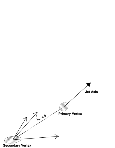
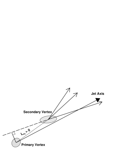
Figure 3: Drawing showing reconstructed secondary vertices, illustrating example cases where (a) $L_{xy}<0$ and (b) $L_{xy}>0$.

VI.3 Event Tagging Efficiency

The event tagging efficiency is the efficiency for tagging at least one of the two $b$-jets in a $t\bar{t}$ lepton + track event using the secvtx tagger. To find the event tagging efficiency we use a $t\bar{t}$ pythia Monte Carlo sample with $m_{t}=175~{}\mathrm{Ge\kern-1.00006ptV}/c^{2}$, the same sample used to calculate the pretag acceptance. Corrections to the event tagging efficiency are made for two effects. The first correction accounts for our ability to reconstruct jets which correspond to a $B$ hadron decay. The second correction is for the possibility of mistakenly tagging light quark jets as heavy flavor jets.

The event tagging efficiency is given by the formula

$$\epsilon_{\textrm{\tiny{tag}}}={\epsilon_{b}^{\prime}}\,F_{1b}+2{\epsilon_{b}^{\prime}}(1-\epsilon_{b}^{\prime})\,F_{2b}+(\epsilon_{b}^{\prime})^{2}\,F_{2b}.$$ (6)

where $\epsilon_{b}^{\prime}$ is the corrected single jet tagging efficiency (see below), and $F_{1b}$ and $F_{2b}$ are the taggable jet fractions. The taggable jet fractions describe the fraction of events with one or two jets which originate with the hadronization of a $b$ quark and might be tagged. The denominator contains events from the simulated $t\bar{t}$ sample which pass the lepton + track selection, including the $\geq 2$ jet requirement. The numerator of $F_{1b}$ is the number of those which have one jet which is matched to a $b$ hadron at generator level and contains two or more tracks passing the secvtx quality requirements described in Section VI.2. The numerator of $F_{2b}$ is the number with two such jets. See Table 4 for the values of the taggable jet fractions.

The single jet tagging efficiency $\epsilon_{b}$ is the ratio of the number of taggable jets with a positive secvtx tag to the number of taggable jets. We multiply $\epsilon_{b}$ by a scale factor, $\epsilon_{\textrm{\tiny{SF}}}$ to account for differences in the single jet tagging efficiency between observed and simulated data. We also apply corrections for the efficiency to tag light quark jets $\epsilon_{q}$, and the efficiency to match a jet to a $b$ hadron decay $\epsilon_{\textrm{\tiny{bmatch}}}$. The corrected single jet tagging efficiency is:

$$\epsilon_{b}^{\prime}=\frac{\epsilon_{b}\,\epsilon_{\textrm{\tiny{SF}}}\,\epsilon_{\textrm{\tiny{bmatch}}}}{(1-\epsilon_{q})}\ \rm{.}$$ (7)

The $\epsilon_{\textrm{\tiny{bmatch}}}$ correction accounts for the situation in which a $b$ quark fragments to produce a jet which does not pass the jet selection criteria employed in this analysis. We measure the efficiency for matching a $B$ hadron to a reconstructed jet in simulated $t\bar{t}$ events. We find $\epsilon_{\textrm{\tiny{bmatch}}}=(98.89\pm 0.04)$ %. We multiply the per jet tagging efficiency obtained above by the matching efficiency to account for this small $b$-jet reconstruction inefficiency.

The last correction, $1/(1-\epsilon_{q})$, accounts for tags of light quark jets, which results in an enhancement to the single jet tagging efficiency. As stated in Section VI.2, negative tags are interpreted as mistakes made by the tagging algorithm, and are due to resolution effects. The negative tagging rate is similar for long-lived $b$-jets and for light quark jets. So, to find the efficiency for tagging light quark jets in $t\bar{t}$ decays, we find the efficiency for negative tags in $b$-jets in pythia $t\bar{t}$ simulation events, which is equivalent to the rate of tagging of light quark jets. We find $\epsilon_{q}=(1.3\pm 0.1)$ %. To correct the single jet tagging efficiency for the tagging of light quark jets we divide by $(1-\epsilon_{q})$.

Table 4 gives a summary of the inputs used to calculate the final event tagging efficiency and we obtain a value of 0.669$\pm$0.037. This translates into 5.5% systematic uncertainty due to event tagging.

Applying the secvtx tagging algorithm to the jets in the 129 lepton + track candidates, we find 69 events with one or more tagged jets.

Quantity	Value
$F_{1b}$	0.	321 $\pm$	0.003
$F_{2b}$	0.	611 $\pm$	0.003
$\epsilon_{b}$	0.	591 $\pm$	0.002
$\epsilon_{\textrm{\tiny{SF}}}$	0.	94 $\pm$	0.06
$\epsilon_{q}$	0.	013 $\pm$	0.001
$\epsilon_{\textrm{\tiny{bmatch}}}$	0.	9889 $\pm$	0.0004
$\epsilon_{\textrm{\tiny{tag}}}$	0.	669 $\pm$	0.037

Table 4: Inputs and results of calculation of event tagging efficiency. Note that the uncertainty on the event tagging efficiency is dominated by the systematic uncertainty on $\epsilon_{SF}$. The other quoted uncertainties are all statistical uncertainties from simulation and are negligible.

VII Background Estimation in Pretag Sample

Background events in the $t\bar{t}$ dilepton sample generally have one or two massive vector bosons decaying to leptons. Non-negligible background processes are $W$ + jets and similar events where one of the jets is misidentified as a lepton, diboson production, and Drell-Yan events where ${\not\!\!E_{T}}$ is produced by a combination of $\tau$ decays and the mismeasurement of the energy of one or more objects in the event. Each of these processes requires the production of extra jets to satisfy event selection criteria.

VII.1 Backgrounds with a Jet Misidentified as a Lepton (“Fakes”)

$W\to\ell\nu$ events with extra jets can pass the lepton + track selection if one of the jets is misidentified as a lepton. This can happen if the fragmentation of a parton results in a single charged hadron carrying most of the momentum of the original parton. If a single charged particle carries more than about 90% of the total momentum of all the charged particles produced by fragmentation, it may satisfy the criteria for an isolated track. This is a relatively rare occurrence, but the inclusive $W$ cross section times the branching ratio to leptons is about 2700 pb Abulencia et al. (2007a), as compared to the 6.7 pb cross section for $t\bar{t}$ production. Even though only about one in 500 $W$+jets events will have enough (three) jets to produce a fake lepton and still pass the event selection, it remains the largest single source of background events.

The estimation of the background from events with a fake lepton has three primary components: the rate for the production of $W$ + jets events with the right kinematic features, the probability for a jet to be misidentified as a lepton (the “fake rate”), and the fraction of events in which the fake and true leptons have opposite charge. All present difficulties for the simulation of physics events. The rate for the production of multiple extra jets in addition to a vector boson can in principle be calculated perturbatively, but for large numbers of jets, the complexity of the calculation grows prohibitively, although progress has been made in recent years Mangano et al. (2003). The fake rate is affected by parton fragmentation, a non-perturbative QCD process which is not currently modeled with the needed accuracy. The fragmentation model will also affect the predicted charge correlation between the true and fake leptons. Inaccuracies in the detector simulation further complicate the picture. Therefore, we rely primarily on observed events for the estimate of the fake lepton background, and use simulated events only when it is impossible to isolate the relevant effect in data.

We summarize the calculation of the expected number of background events before describing the individual components in detail. The total number of lepton + track events with $n$ jets where one of the leptons is fake, $N_{\textrm{\tiny{fake}}}^{n}$, is the sum of the number of events $N_{t}^{n}$ with a fake track lepton and the number $N_{\ell}^{n}$ with a fake fully reconstructed lepton, where we use the subscript $t$ to indicate numbers relating to track leptons and $\ell$ to indicate numbers relating to fully reconstructed leptons. The estimates $N_{t}^{n}$ and $N_{\ell}^{n}$ are calculated separately using similar procedures, and then corrected for the efficiencies $\epsilon_{\textrm{\tiny{OS}}}^{n}$ and $\epsilon_{Z}^{n}$ (explained in more detail at the end of this section) of the remaining lepton + track event selection:

$$N_{\textrm{\tiny{fake}}}^{n}=\epsilon_{\textrm{\tiny{OS}}}^{n}\,\epsilon_{Z}^{n}\,(N_{\textrm{\tiny{t}}}^{n}+N_{\ell}^{n})$$ (8)

where

$$N_{t}^{n}=\sum_{E_{T},|\eta|}\left(f_{t}^{(n+1)}(E_{T},|\eta|)\right)\left(N_{j}^{(n+1)}(E_{T},|\eta|)\right)$$ (9)

and

$$N_{\ell}^{n}=\sum_{i=1}^{4}\sum_{E_{T},|\eta|}\left(f_{\ell}^{i}(E_{T},|\eta|)\right)\left(N_{j}^{(n+1)}(E_{T},|\eta|)\right)(A_{\ell}^{i}/A_{t})\ \textrm{.}$$ (10)

To predict the number of events $N_{t}^{n}$ with $n$ jets and a fake track lepton, we multiply the number of jets $N_{j}^{(n+1)}(E_{T},|\eta|)$ in the lepton + ${\not\!\!E_{T}}$ + $(n+1)$ jet sample, binned in jet $E_{T}$ and $|\eta|$, by the track lepton fake rate $f_{t}^{(n+1)}(E_{T},|\eta|)$ for the same number of jets and range of jet $E_{T}$ and $|\eta|$. The result is summed over jet $E_{T}$ and $|\eta|$. The selection for lepton + ${\not\!\!E_{T}}$ + jets events is described in Section VII.1.1, and the fake rate for track leptons is defined in Sections VII.1.3 and VII.1.4 after motivating the choice of the $\gamma$ + jets sample for the fake rate calculation in Section VII.1.2. We test the performance of the track lepton fake rate by comparison among relevant jet samples in Section VII.1.5. To include the contribution from events with a fake fully reconstructed lepton, $N_{\ell}^{n}$, we multiply the same jet distributions $N_{j}^{(n+1)}(E_{T},|\eta|)$ by the fully reconstructed lepton fake rates $f_{\ell}^{i}$, where the index $i$ indicates the type of the lepton identification criteria, and both the fake rate and jet counts are binned in jet $E_{T}$ and $|\eta|$ as for the fake track leptons. This yields the predicted numbers of events with two fully reconstructed leptons where one is real and one is fake. We rescale the result by the ratio of the $W\to\ell\nu$ + jets acceptance $A_{t}$ for track leptons to the acceptance $A_{\ell}^{i}$ for fully reconstructed lepton type $i$, to find the number where the track lepton is the lepton from the $W$ and the fully reconstructed lepton is fake. Summing over the four fully reconstructed lepton types ($i$ runs from 1 to 4) gives the total result. Details on the inclusion of fake fully reconstructed leptons are given in Section VII.1.6.

The dominant contribution to the lepton + ${\not\!\!E_{T}}$ + jets sample is $W$ + jets, but for the sample with three or more jets, which is used in the background prediction for the cross section measurement, there is also a significant contribution from $t\bar{t}$. This happens in the “lepton + jets” decay channel, in which the $W$ that decays to a pair of quarks adds one or two jets to the final state in addition to the two jets from the $b$ quarks. If the lepton from the decay of the other $W$ is reconstructed as an electron or muon and one of the jets in the final state produces an isolated track (or vice versa), such events can pass the full lepton + track event selection. The treatment of the $t\bar{t}$ contribution to the candidates with a fake lepton is discussed in Section VII.1.7. These events require some special care, as they introduce a dependence on the cross section we are measuring. That is treated by explicitly including the dependence in the likelihood used to calculate the cross section (see Section IX.1).

The remaining component of the estimate is the efficiency for the selection criteria that cannot be applied in selecting the lepton + ${\not\!\!E_{T}}$ + jets sample. First is the opposite-charge requirement. We calculate the efficiency $\epsilon^{n}_{\textrm{\tiny{OS}}}$ for this requirement using a combination of observed data and Monte Carlo simulations in Section VII.1.8. The other two requirements are the increased ${\not\!\!E_{T}}$ threshold for events with a lepton + track invariant mass close to the $Z$ resonance, and the track lepton-${\not\!\!E_{T}}$ opening angle veto. The efficiencies for these, collectively labeled $\epsilon_{Z}^{n}$ in Eq. 8, are given in Section VII.1.9.

Finally, we tally the systematic uncertainties on this background estimate in Section VII.1.10.

VII.1.1 Selection of $W$ + jets Events

The selection for $W$ + jets events in the data is based on the event selection described in Section IV, with all requirements involving the track lepton omitted. That is, we select events from the same high-$p_{T}$ electron and muon trigger sample containing the signal candidates, with one fully reconstructed electron or muon. We also require that these events have ${\not\!\!E_{T}}$ $>25\ \mathrm{Ge\kern-1.00006ptV}$ and pass the $\Delta\varphi$ criteria for the fully reconstructed lepton and the jets. Since one of the jets will be reconstructed as a lepton in events with a fake lepton, we predict the number of events passing the full lepton + track selection and having $N$ jets by using events with $N+1$ jets. We count the number of events with one jet, two jets, or at least three jets.

The largest contribution to this sample is $W$ + jets, where the $W$ decays leptonically. There is also a significant contribution from $t\bar{t}$, which will be discussed in more detail below. There is also a small contribution from pure-QCD multijet events where one of the jets has been wrongly identified as a fully reconstructed electron or muon.

VII.1.2 Jet Properties Influencing the Fake Rate

To motivate the choice of the $\gamma$ + jets sample for the fake rate, we focus our attention on the largest contribution to the fake lepton background, $W$ + jets events. The lepton fake rate is determined by parton fragmentation, and fragmentation is determined by the energy and type of the parton. The energy dependence will be included by parameterizing the fake rate as a function of jet $E_{T}$ and $|\eta|$. Here we consider the possible influence of the parton type.

A jet produced in association with a $W$ has a higher probability of being a quark jet, meaning a jet which originates from a quark, than a jet of the same energy produced in a generic QCD multijet event. To understand this, note that most $W$ and multijet production at the Tevatron takes place at relatively low $x$, where $x$ is the fraction of the proton momentum carried by an individual parton. For $Q^{2}$ values typical of $W$ + jets or multijet production at the Tevatron, the gluon PDF is strong relative to the valence quark PDFs for $x\lesssim 0.15$. The two leading diagrams for $W$ + 1 jet production (see Fig. 4) at the Tevatron have the same amplitude. The preference for diagrams with incoming gluons implies that the diagram with an outgoing quark will prevail, so the jets associated with a $W$ boson are more likely to be quark jets. This preference for quark jets is even more marked in $\gamma$ + jets samples because the photon is massless, so we sample an even lower-$x$ part of the PDF. In the case of multijet production, the leading order diagram for $gg\to gg$ has a larger amplitude than any of the other leading order $2\to 2$ diagrams containing other permutations of light quarks and gluons. Taking that in combination with the strength of the gluon PDF, one expects jets produced in pure strong interaction events to be predominantly gluon jets, that is, jets originating from gluons.

Figure 4: Leading diagrams for $W$ and $\gamma$ production with one associated jet at the Tevatron. Diagrams (a) and (b) are for $\gamma$ + 1 jet production, and (c) and (d) are for $W$ + 1 jet production. Diagrams (a) and (c) dominate because of the relative strength of the gluon PDF at low $x$.

The different partonic origins of jets matter because jets from light quarks appear to have a different fake rate than jets from gluons. Gluon fragmentation results, on average, in a larger number of charged particles than quark fragmentation. This behavior has been verified experimentally, and can be seen in simulation Affolder et al. (2001). An immediate consequence is the fact that a quark jet will be more likely than a gluon jet to contain a single charged track carrying most of the parton’s energy. This also implies an increased probability to produce a fake lepton.

We can test the partonic origins of the jets in different processes and their effect on fake rates using simulated data. In simulation, it is possible in most cases to match a reconstructed jet to the quark or gluon from which it most likely developed. While we do not trust the absolute value of fake rates in simulation, relative comparisons are still meaningful. First, we find the fraction of jets matched to a quark in simulated $\gamma$ + jets, $W$ + jets, and QCD multijet events. All of these samples are generated using pythia, as described in Section III. The minimum photon $E_{T}$ in the photon sample is 22 $\mathrm{Ge\kern-1.00006ptV}$ and we select events with reconstructed photon $E_{T}>25\ \mathrm{Ge\kern-1.00006ptV}$. The minimum parton $p_{T}$ in the jet sample is 18 $\mathrm{Ge\kern-1.00006ptV}/c$. The quark jet fractions for all of these processes as a function of jet $E_{T}$ are shown in Fig. 5. For any choice of jet multiplicity, the fraction of jets which are from quarks is highest in the photon sample, next highest in the $W$ sample and smallest in the multijet sample. Also note that in the $W$ and photon samples with higher jet multiplicities, the tendency toward quark jet dominance persists but is diminished by the enhanced impact of higher-order processes. Finally, one also sees that with increasing jet $E_{T}$, the preference for quark jets in multijet events increases. This is also to be expected given the increased $Q^{2}$ of the interaction and hence a reduced probability of an initial $gg$ interaction.

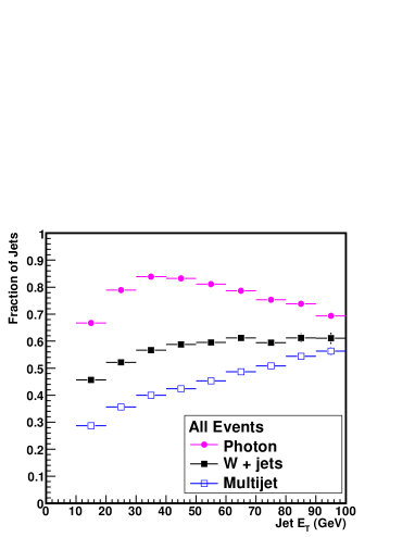
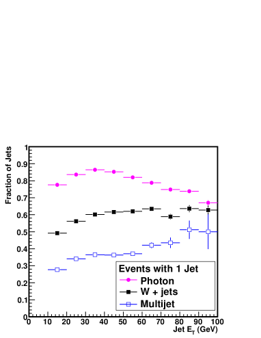
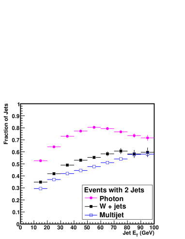
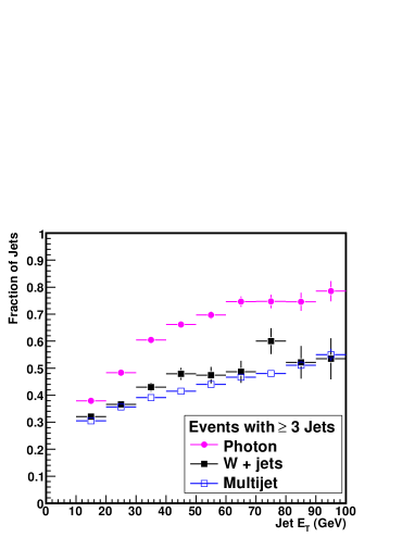
Figure 5: The fraction of jets matched to a quark in simulated photon (filled circles), $W$ (filled squares) and multijet (open squares) events, as a function of jet $E_{T}$. The fraction is shown for events with any number of jets (a), and then separately for events with one (b), two (c), and at least three (d) jets.

Figure 6 shows the difference in the fake rates between the three jet samples considered earlier: $\gamma$ + jets, $W$ + jets, and QCD multijet. The $\gamma$ + jets sample has the highest fraction of quark jets (See Fig. 5), followed by the $W$ + jets and multijet samples, and their fake rates follow the same pattern. Figure 6 also shows that, in simulated multijet events, the quark jet fake rate is nearly an order of magnitude higher than the gluon jet fake rate. Combined with the different propensities for producing quark jets, this leads to different fake rates in different samples. We also compare the separated quark and gluon jet fake rates for the three samples in Fig. 6, and observe that the agreement between the separated fake rates is better than the agreement between the inclusive ones.

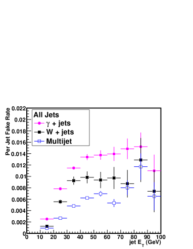
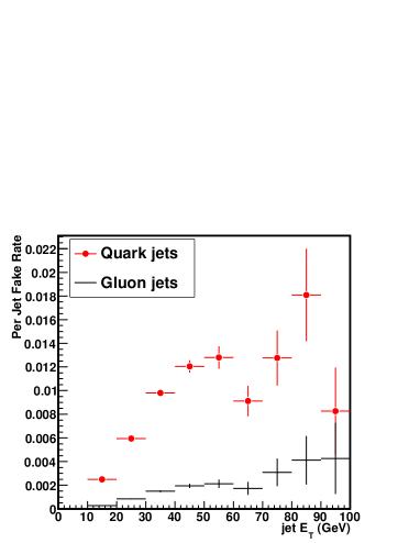
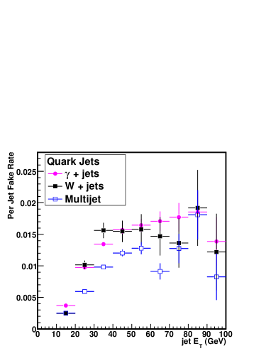
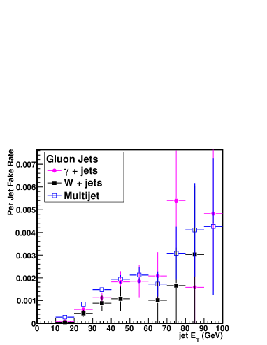
Figure 6: Track lepton fake rates in simulation as a function of denominator jet $E_{T}$. (a) Fake rate for all jets in simulated $\gamma$ + jets, $W$ + jets, and multijet events. The fake rate in multijet events is lower than the fake rate in $W$ + jets events, and both are lower than that in $\gamma$ + jets events. Note that this $\gamma$ + jets sample does not have the $E_{\gamma}>80\ \mathrm{Ge\kern-1.00006ptV}$ requirement applied. (b) Fake rate for jets matched to quarks (“quark jets”) compared to the fake rate for jets matched to gluons (“gluon jets”), showing the disagreement between them. Fake rates taken from the simulated multijet sample. (c) Fake rates for quark jets in the three samples. The agreement is better than that observed in (a). (d) The same, but for jets matched to gluons.

VII.1.3 Fake Rate Definition

The track lepton fake rate is the number of isolated tracks, divided by the number of jets, in a sample containing no true leptons. The numerator is the number of track leptons according to the definitions in Section IV.3. The denominator is the number of jets according to the definition in Sec. IV.4. Recall that in addition to the standard calorimeter cluster-based jets, this jet collection includes tracks not associated with a jet as well as jets containing a high-$p_{T}$ track which otherwise would have fallen below the jet selection $E_{T}$ threshold. The jets used in constructing the fake rate are identical to those used to count jets for candidate event selection. Note that a fake track lepton is a true isolated track, but one that does not originate from a lepton.

Ideally, the fake rate is measured in a data sample where the contamination from true leptons is negligible. For this analysis, we use a sample of events triggered by a photon with $E_{T}>25$ $\mathrm{Ge\kern-1.00006ptV}$. Photons are restricted to the central calorimeter and selected with criteria similar to those used for electrons, except that there must be no track pointing at the energy deposited in the electromagnetic calorimeter Abulencia et al. (2007b). To further reduce the possibility of lepton contamination, we exclude events in which the invariant mass of the photon and any jet in the event is close to the $Z$ resonance ($76~{}\mathrm{Ge\kern-1.00006ptV}/c^{2}<M<106~{}\mathrm{Ge\kern-1.00006ptV}/c^{2}$) when the jet is a track or has more than about 90% of its energy in the electromagnetic calorimeter. Finally, we require the photon to have at least 80 $\mathrm{Ge\kern-1.00006ptV}$ of energy (not $E_{T}$), to strengthen the analogy to $W$ production through the required $Q^{2}$.

The fake rate depends strongly on the $E_{T}$ and $|\eta|$ of the jets in the denominator, so we parameterize it as a function of these quantities. The fake rate for track leptons for each jet multiplicity is shown as a function of the $E_{T}$ and $|\eta|$ of the denominator jets in Fig. 7.

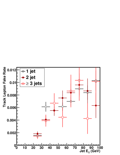
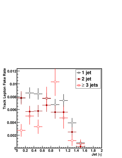
Figure 7: Track lepton fake rates as a function of $E_{T}$ (a) and $|\eta|$ (b) of the faking jet. The fake rate is the probability for a jet to pass the track lepton identification requirements, including the track isolation. The fake rate is measured in jets from photon + jets data, and includes $Z$ + 1 jet events in the 1 jet fake rate. The uncertainty is statistical only. See Section VII.1.3 for details.

Taking the jets for the lepton fake rate from a photon-triggered data sample instead of a jet-triggered has not been done before in a dilepton $t\bar{t}$ cross section measurement. The Run I dilepton cross section measurement Abe et al. (1998) and the Run II measurement with 200 pb^-1 of integrated luminosity Acosta et al. (2004) both used samples triggered by high-$E_{T}$ jets. The Run I measurement placed an uncertainty of 62% on the fake lepton background. In the two measurements of the previous Run II result, the uncertainty on the fake lepton background is 30% for the earlier version of this analysis, and 51% for the analysis using two fully reconstructed leptons. The uncertainty on the fake lepton background for this analysis will be described in detail at the end of this section, but it is a total of 20%, with 6% from the statistical uncertainty. The previously published measurements have a factor of 5 to 10 less integrated luminosity, so the statistical uncertainty would have made this technique impractical in earlier measurements. As an aside, it is because of the availability of larger data samples that the failings of fake rates calculated with jet-triggered samples have started to become apparent. We also note that our initial attempts to improve the fake lepton background estimate were based on adding a third parameter, such as the number of tracks per jet, to the fake rate. This technique was dropped in favor of the one presented here because it was less successful when tested in simulation.

VII.1.4 Use of $Z$+jets Data

In photon plus one jet events, conservation of momentum implies that events where the measured $E_{T}$ of the balancing jet is significantly lower than the photon $E_{T}$ are rare. Because of this, there are very few events in the lowest $E_{T}$ bins of the fake rate. This is not crucially important since this is an input to the zero jet event count prediction, which does not enter into the cross section calculation. Nevertheless, it is possible to fill the gap in the one jet fake rate by including the $Z$ + 1 jet sample. The $Z$ + jets sample is a near-perfect analog to the $W$ + jets sample, up to the slight difference in mass scale. Most $Z$ + jets events have at most one jet, typically near the $E_{T}$ threshold, so there is not enough data to make useful measurements of lepton fake rates for higher jet multiplicities. But, one-jet events where the jet is in the lower $E_{T}$ range is exactly what $\gamma$ + jets events are lacking. Therefore, the total rate used to predict the number of fake leptons in the zero-jet lepton + track sample is the combined rate from the $\gamma$ + 1 jet and $Z$ + 1 jet samples. We combine the two fake rates by adding the jets from the $Z$ + 1 jet numerator (denominator) to the $\gamma$ + 1 jet numerator (denominator) before calculating the fake rate.

VII.1.5 Validation of Track Lepton Fake Rate

We test the accuracy of the track lepton fake rate in both real and simulated data. To increase the size of the sample for validation, a lower kinematic threshold of 15 $\mathrm{Ge\kern-1.00006ptV}$ is used for both the track leptons and jets. This adds jets to the sample because of the steep falloff of the $E_{T}$ distribution. Also, the fake rate for 15 $\mathrm{Ge\kern-1.00006ptV}$ track leptons is higher than for 20 $\mathrm{Ge\kern-1.00006ptV}$ track leptons, because it corresponds to a larger portion of the fragmentation spectrum.

Using simulated CDF data, it is possible to test the fake rate estimation procedure by using the fake rates obtained from simulated $\gamma$ + jets events to predict the number of fake leptons in simulated $W$ + jets events. Events with 0, 1, and $\geq$ 2 jets in addition to the fake lepton are considered. Figure 8 shows the predicted and observed number of fake track leptons as a function of the $E_{T}$ of the misidentified jet, for each jet multiplicity. The integrated results are provided in Table 5. The fake rate from jets associated with an 80 $\mathrm{Ge\kern-1.00006ptV}$ photon is seen to overestimate the number of fake leptons observed in jets associated with a $W$. This effect is only statistically significant in events with one jet, and we will include this 18% discrepancy in the systematic uncertainty on this background. Omitting the $Z$ + 1 jet data from the fake rate only exacerbates the disagreement (The previous section describes the use of the $Z$ + jets data in the one jet fake rate).

We directly test the fake rate obtained from the photon data using $Z$ + jets data. The number of isolated tracks predicted in the $Z$ + jets data is compared to the number observed for events with 0, 1, and $\geq 2$ jets in addition to the isolated track. For this test, only the fake rate from $\gamma$ + 1 jet events is used to predict the number of fake leptons coming from the $Z$ + 1 jet sample. Although the event sample is small, no statistically significant discrepancy is observed for any jet multiplicity in this test. Figure 9 shows the predicted and observed number of isolated tracks as a function of the $E_{T}$ of the jet, for each jet multiplicity. Table 5 provides the integrated results. The integer number of isolated tracks is well-predicted, and the shape of the isolated track $p_{T}$ distribution is well-modeled for events with zero or one jets in addition to the isolated track. The agreement between the predicted and observed distributions in the two-or-more jet case is more difficult to assess. There are 2358 $Z$ events with three jets, so the predicted distribution is smooth, but there are only thirteen $Z$ candidates with two jets and an isolated track, so the distribution of the $p_{T}$ of the isolated tracks is highly prone to statistical fluctuations.

We use the same framework to test fake rates obtained from multijet events. To mimic the fake rate used in the previous published version of this analysis, we simulate the requirements of the 50 $\mathrm{Ge\kern-1.00006ptV}$ jet trigger at CDF on a pythia multijet sample produced requiring a minimum parton $p_{T}$ of 18 $\mathrm{Ge\kern-1.00006ptV}/c$. The fake rate is constructed as described above, except that events with any number of jets are included. The inclusive jet fake rate is then applied to jets from simulated $W$ + jets events. The results are shown next to the prediction from the photon + jets fake rate in Fig. 8. For $W$ + 1 jet events, 3040 $\pm$ 350 events are predicted, and 4480 are observed. Using the same logic as used to derive the 18% systematic uncertainty quoted above, this corresponds to a 47% systematic uncertainty for the fake rate from data collected using a jet trigger. This motivates the choice to use the jets from the photon trigger sample to build the fake rate.

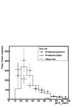
Figure 8: Predicted and observed number of fake track leptons in simulated $W$ + jets events, as a function of jet $E_{T}$. The comparison is made for events with zero (a), one (b), and at least two (c) jets in addition to the one that is reconstructed as an isolated track. One prediction, shown as solid squares, is made using the a fake rate derived from simulated $\gamma$ + jets and $Z$ + jets events, exactly as the fake rate is constructed from the observed data. The other, shown as open circles, is made using a fake rate derived from simulated QCD multijet events. Uncertainties on the predictions are statistical only.

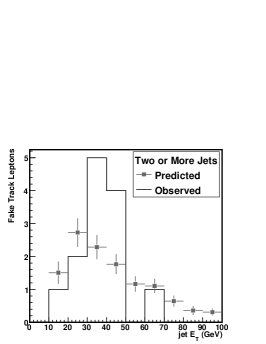
Figure 9: Predicted and observed number of isolated tracks observed in CDF $Z$ + jets data, as a function of jet $E_{T}$. The comparison is made for events with zero (a), one (b), and at least two (c) jets in addition to the one that is reconstructed as an isolated track. The fake rate used is derived from $\gamma$ + jets data, and the uncertainty on it is statistical only.

Predict $W$ + jets with $\gamma$ and $Z$ + jets:

Test in simulated data

	Predicted	Observed
1 jet	5473 $\pm$ 147	4480
2 jets	1332 $\pm$ 200	1047
$\geq$ 3 jets	304 $\pm$ 67	226

Predict $Z$ + jets with $\gamma$ + jets:

Test in CDF data

	Predicted	Observed
1 jet	100 $\pm$ 13	101
2 jets	28 $\pm$ 2	26
$\geq$ 3 jets	12 $\pm$ 1	13

Table 5: Predicted and observed number of isolated tracks of hadronic origin in tests performed in observed and simulated data. The number of jets quoted is in addition to the jet which is reconstructed as an isolated track. The only statistically significant discrepancy observed is in the one jet category in the simulation, and is taken as part of the basis of the systematic uncertainty on this background estimate. Note that in the column headings, “Observed” refers to the directly counted isolated tracks, regardless of whether the study is done in real or simulated data.

VII.1.6 Fake Rates for Fully Reconstructed Leptons

We also measure fake rates for all four primary lepton types, using the same method and data as is used for the track leptons. The fake rate is at least an order of magnitude smaller for primary leptons than for track leptons. Because there are so few events in the numerator of the fake rate for the primary leptons, we use an inclusive fake rate instead of calculating it separately for events with different numbers of jets. The fake rates for the fully reconstructed leptons, as a function of the $E_{T}$ and $|\eta|$ of the denominator jets, are shown in in Fig. 10.

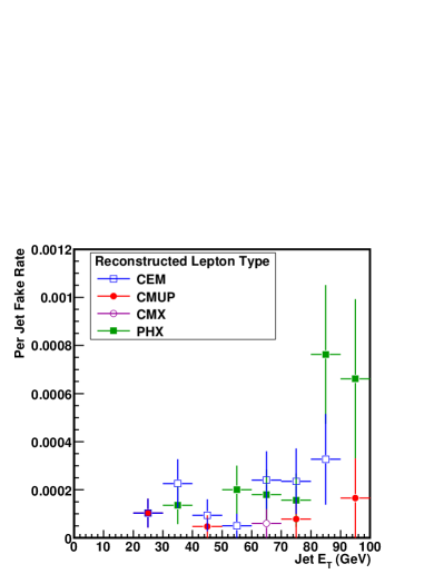
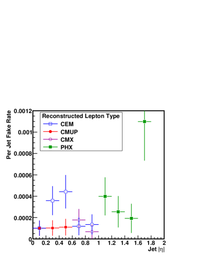
Figure 10: Fully reconstructed lepton fake rates as a function of $E_{T}$ (a) and $|\eta|$ (b) of the jet in the denominator. The fake rate is the probability for a jet to pass the lepton identification requirements and is measured in jets from photon + jets data. The shown uncertainty is statistical only.

To find the number of events where the track lepton is the lepton from the $W$ and the fully reconstructed lepton is fake, we multiply the fully reconstructed lepton fake rates by the jet $E_{T}$ and $|\eta|$ distributions from the lepton + ${\not\!\!E_{T}}$ + jets data described in Section VII.1.1. That gives the number of events with two fully reconstructed leptons where one is fake. To find the number where the true lepton is the track lepton, we scale the number by the ratio of the $W\to\ell\nu$ + jets acceptance for track leptons to the acceptance for fully reconstructed leptons. This ratio is measured in $W$ + jets events simulated using pythia. There are other sources of fake leptons in the sample, but $W$ + jets is the dominant contribution, and the ratio of the acceptances for the sub-dominant contribution from $t\bar{t}$ should be similar, since the real lepton is still from a $W$. Summing over all lepton types yields the total contribution from fake fully reconstructed leptons, which are 6% of the total fake lepton background.

VII.1.7 Contribution from $t\bar{t}$ Events with a Fake Lepton

Other than $W$ + jets, the only process contributing significantly (more than 5%) to the lepton + ${\not\!\!E_{T}}$ + jets data sample is $t\bar{t}$ lepton + jets events. For a top quark mass of 175 $\mathrm{Ge\kern-1.00006ptV}/c^{2}$, corresponding to a cross section of 6.7 pb, such events produce 19% of the jets in the lepton + ${\not\!\!E_{T}}$ sample with three or more jets, the sample used derive the fakes contribution to the background for the cross section measurement. Lepton + jets $t\bar{t}$ events make a negligible contribution to lepton + ${\not\!\!E_{T}}$ samples with one or two jets. Single top quarks, produced through the electroweak interaction, can also generate the required lepton, ${\not\!\!E_{T}}$, and jets signature, but the small cross section and lower jet multiplicity at leading order mean that their contribution is negligible.

Because of its size, the lepton + jets $t\bar{t}$ contribution deserves separate consideration. Study of simulated $t\bar{t}$ events indicates that over 90% of the jets in these events come from quarks. This is a very different fraction than for any other sample considered, although many (roughly 2/3) of the jets are from heavy quarks, such as a $b$ from $t$ decay or a $c$ from $W$ decay. The track lepton fake rate for jets from a light quark is about twice the rate for jets from a heavy quark, because the latter typically produce a larger number of charged tracks, leading to a greater likelihood to fail the track isolation criteria. As a result, the fake lepton is associated with the jet produced by a quark from $W$ decay in about 90% of the simulated events with a fake lepton.

The fake rate designed for $W$ + jets events is still usable. First, the smaller probability that heavy quark jets will be manifested as isolated tracks partially compensates for the fact that there are fewer gluon jets in $t\bar{t}$ than in the photon plus jets data used to define the fake rate. Second, the contribution of $t\bar{t}$ is still relatively small compared to $W$ + jets and the large systematic on the fake rate due to the discrepancy in the single jet bin is adequate to cover any remaining difference. We test the validity of these statements using the fake rates from the simulated $W$ + jets sample, because there is an insufficient number of events in the simulated $\gamma+\geq 3$ jet sample to make a meaningful comparison. If the $W$ + jets fake rate is sufficiently similar to the one from $t\bar{t}$ lepton + jets events, we may still use the same fake rate for both. The fake rate from the $W$ + jets sample predicts 518 $\pm$ 45 isolated tracks in a simulated $t\bar{t}$ lepton + jets sample, in which 424 are actually observed. The level of disagreement (18%) is not egregious when compared to the statistical uncertainty, and is comparable to the systematic uncertainty. We therefore use the photon + jets fake rate to predict the number of fake leptons for all events passing the $W$ + jets selection, regardless of their source.

VII.1.8 Fraction of Events having Opposite Sign Leptons

We must also estimate the fraction of events with a fake lepton in which the real and fake lepton have opposite sign. This fraction is different for $W$ + jets and $t\bar{t}$ events, so they must be considered separately.

First we will consider the opposite-sign fraction for $W$ + jets events. Leading diagrams for $W$ + jets production have the $W$ recoiling against a quark which becomes a jet in the event, so the charge of the tracks in that jet is expected to be anti-correlated with the charge of the $W$.

In simulated $W$ + jets events, the charge correlation is large, but falls off with increasing jet multiplicity. We measure opposite-sign fractions of 81 $\pm$ 3% for events with zero jets, 73 $\pm$ 2% for events with one jet, and 75 $\pm$ 5% for events with at least two jets. The difficulty with the numbers from the simulation is that the charge correlation, like the fake rate, is influenced by details of jet fragmentation that may not be fully taken into account in the Monte Carlo simulations. The opposite-sign fractions can be checked in candidate lepton + track events with no jets, where the contribution from $t\bar{t}$ is negligible but where the expected contribution of events with a fake lepton is large. Prior to an opposite-sign requirement, the total number of predicted events agrees with the number observed, within the statistical uncertainty. When the predicted opposite-sign fraction from simulation is applied, more same-sign events are observed than are predicted, and the number of opposite-sign events observed is correspondingly too small compared to the prediction. This suggests that the simulation overestimates the fraction of events with a fake lepton of opposite charge. We therefore obtain the opposite sign fraction from observed data, using the zero-jet candidate events. We can further enhance the fraction of events with a fake lepton by requiring a significant amount of energy in the region of the hadronic calorimeter at which the track points. This is about 70% efficient for events with a fake lepton and $Z/\gamma^{\star}\rightarrow\tau\tau$ events, but reduces all other contributions by an order of magnitude. We then subtract the estimated number of events from sources with two real leptons for all events and for those with opposite sign. We find that 67 $\pm$ 3% of remaining events are opposite-sign, which is taken to be the opposite-sign fraction for all events with zero jets.

As a cross-check, we also measure the opposite-sign fraction using the zero-jet events without the hadronic energy requirement described above, and find 69 $\pm$ 5%, in good agreement with the number calculated with the requirement. The larger uncertainty is due to the systematic uncertainties on the larger contributions to the zero-jet sample from the other processes.

We cannot apply the same procedure to derive the opposite-sign fraction for higher jet multiplicities because the contribution from $t\bar{t}$ is non-negligible. To obtain the charge correlation for events with more jets, we rely on the simulation to model the dependence of the correlation on the number of jets in the event. The assumption made is that each additional jet dilutes the opposite-sign fraction toward 50%, the fraction corresponding to no correlation. Defining a dilution factor $x$, the opposite-sign fraction $f_{i+1}$ of events with $i+1$ jets can be expressed in terms of the fraction $f_{i}$ for events with $i$ jets as

$$f_{i+1}=0.5x+f_{i}(1-x)\ .$$ (11)

From the (81 $\pm$ 3)% and (73 $\pm$ 2)% figures, we find $x=(26\pm 12)$%. Applying this to the (67 $\pm$ 3)% fraction from the zero-jet events, we find an opposite-sign fractions of (63 $\pm$ 3)% for events with one jet. Repeating the procedure with the same $x$ and the one-jet opposite-sign fraction, we find (59 $\pm$ 3)% for events with two or more jets.

Turning to the case of $t\bar{t}$ lepton + jets events with a fake track lepton, we observe in simulation that 79% of such events have opposite-sign leptons. It seems likely that the charge correlation here is attributable to the fact that the summed charge of the quark pair produced by the $W$ will be the opposite sign of the charge of the lepton from the other $W$. We prefer not to use the number from simulation directly, since our results in the $W$ + jets sample suggest that the fragmentation model in simulation tends to overestimate charge correlations. We correct the result from simulation using the observed difference between observed and simulated data for $W$ + 1 jet events where the jet is reconstructed as an isolated track, using the same method described in the previous paragraph. In simulation, 81% of events are opposite-sign, compared to the 67% in the CDF data. For $t\bar{t}$ lepton + jets events with three or more jets, we scale the fraction from simulation to (67 $\pm$ 6)%, which is higher than the fraction for $W$ + jets events with the same number of jets. The uncertainty is taken to be half the difference between the original and rescaled numbers, or 9%. The statistical uncertainties on the fractions from simulation are less than a percent and negligible in comparison.

To obtain a fake lepton background prediction for events with two or more jets, we must combine the two opposite-sign fractions obtained for $W$ + jets and $t\bar{t}$ lepton + jets in proportion to the estimated number of fake leptons contributed by each process. Because the predicted fraction of $t\bar{t}$ in the $W$ + jets data is based on an acceptance measured in simulation, this introduces a dependence on the $t\bar{t}$ cross section. We remove this dependence by including it explicitly in the pretag background calculation in the likelihood expression used to measure the cross section, which will be described in more detail in Section IX.1. The result is that, for the measured cross section of 9.6 pb, (27 $\pm$ 4)% of jets in the normalizing $W$ + jets sample are predicted to be from $t\bar{t}$ for the final cross section value, and the re-weighted opposite-sign fraction is (61 $\pm$ 3)%. Note that the 27% is calculated from the measured $t\bar{t}$ cross section and is in a sense the result of the fit, so the uncertainty on it is the observed change in the fraction when the cross section is varied by its calculated uncertainties.

VII.1.9 Efficiency for Additional Selection

We measure the efficiency of the $Z$ veto and the track lepton $\Delta\varphi$ requirement in simulated $W$ + jets events generated using alpgen+pythia Monte Carlo. The efficiency for the two criteria is (82 $\pm$ 2)% for events with zero jets, (85 $\pm$ 1)% for events with one jet, and (89 $\pm$ 2)% for events with two or more jets. Scaling the event counts by these efficiencies yields the final prediction of candidate events with a fake lepton as a function of the number of jets.

VII.1.10 Systematic Uncertainties

There are three sources of uncertainty in the estimate of the background from events with a fake lepton: the statistical uncertainty on the fake rate, the systematic uncertainty on the overall normalization of the estimate, and the uncertainty on the fraction of events with a fake lepton where the leptons have opposite sign.

The uncertainty on the overall normalization comes from the largest observed discrepancy in the simulated and observed data tests described above. We have also argued that this 18% uncertainty covers possible discrepancies between the fake rate for jets in $W$ + jets events and jets in $t\bar{t}$ lepton + jets events. The uncertainty on the opposite-sign fraction is the statistical uncertainty on the fraction calculated from zero-jet candidate data, combined with the systematic uncertainty from the scaling of the fraction for $t\bar{t}$ lepton + jets events, and is 5%.

Combining the 18% and 5% systematic uncertainties with the 6% statistical uncertainty, the total uncertainty on this background is 20%.

VII.2 Diboson

VII.2.1 Diboson Acceptance

Diboson events ($WW$, $WZ$, and $ZZ$) events have small cross sections, comparable to the $t\bar{t}$ cross section. It is only recently that CDF and DØ have obtained sufficient data to observe $WZ$ production Abulencia et al. (2007c); Abazov et al. (2007c) and $ZZ$ production Aaltonen et al. (2008c); Abazov et al. (2008d). Also, if one or both bosons decay to leptons, these events can mimic the $t\bar{t}$ signature, so it is not possible to isolate a large sample of such events in the data. Therefore, the acceptance calculated from simulated events is used together with the theoretical production cross sections to estimate this background. We use event samples generated with the pythia Monte Carlo generator and apply the same corrections to the diboson acceptance as we did for the signal acceptance, with one additional correction for the rate of jet production, described below. The estimated number of events in the candidate sample is then the corrected acceptance multiplied by the theoretical cross section and the integrated luminosity. The theoretical cross sections for these processes are 12.4 $\pm$ 0.8 pb for $WW$, 3.7 $\pm$ 0.3 pb for $WZ$, and 3.7 $\pm$ 0.3 pb for $ZZ$ Campbell and Ellis (1999). The $ZZ$ sample includes the $\gamma^{*}$ contribution, with $M_{Z/\gamma^{*}}>2\ \mathrm{Ge\kern-1.00006ptV}/c^{2}$ for both bosons. These cross sections are calculated using the MCFM Monte Carlo program Campbell and Ellis (1999) and the uncertainties are based on the $Q^{2}$ and PDF dependence of the cross sections.

VII.2.2 Correction for Number of Jets

pythia is a leading order Monte Carlo program and so is not expected to correctly predict the fraction of events with extra high-$p_{T}$ jets in addition to the core process. A scale factor derived from a comparison of jet production in real and simulated $Z$ + jets data is applied to correct the acceptance for events with two or more jets up to the observed level. A sample of $Z$’s are selected with two opposite-charge, fully reconstructed electrons or muons having an invariant mass in the interval $76~{}\mathrm{Ge\kern-1.00006ptV}/c^{2}<M<106~{}\mathrm{Ge\kern-1.00006ptV}/c^{2}$. The fraction of events with two or more jets in simulation, 0.0142 $\pm$ 0.0002, is lower than the fraction observed in data, 0.0153 $\pm$ 0.0008. A scale factor, once again defined as the ratio of the fraction in observed data to the fraction in simulated data, is calculated for each jet multiplicity. The scale factors found are 1.006 $\pm$ 0.002 for events with zero jets, 0.940 $\pm$ 0.018 for events with one jet, and 1.08 $\pm$ 0.06 for events with two or more jets, where the uncertainties are statistical only. We then multiply the acceptance by the appropriate scale factor for each jet multiplicity. In order to maintain the same overall normalization, we rescale all three acceptances by a common factor so that their sum is unchanged.

VII.2.3 Systematic Uncertainties

The systematic uncertainties relevant to the signal acceptance also apply here. The lepton identification uncertainties are still 1.1% for both fully reconstructed and track leptons. The uncertainty on the number-of-jets correction, 5.5%, also applies to the predicted number of events. The jet energy scale uncertainty is also relevant here, and is evaluated in the same way, but has a larger effect: the energy spectrum of radiated jets falls sharply, so that small changes in the jet energy can lead to large changes in the event selection efficiency. The resulting uncertainty is 5.8%. Finally, we also include the theoretical uncertainties on the cross sections used to normalize the background prediction, which are 6% for the $WW$ and 7% for $WZ$ and $ZZ$. The total uncertainty on the diboson background calculation is 11%.

VII.3 Drell-Yan

Drell-Yan events with ${\not\!\!E_{T}}$ are a significant source of background for $t\bar{t}$ lepton + track events since there are two real leptons in the final state and the inclusive cross section is large ($\sigma(p\bar{p}\to Z/\gamma^{\star})\times Br(Z/\gamma^{\star}\to\ell^{+}\ell^{-})=251\pm 5$ pb for $66\ \mathrm{Ge\kern-1.00006ptV}/c^{2}<M_{\ell\ell}<116\ \mathrm{Ge\kern-1.00006ptV}/c^{2}$ Abulencia et al. (2007a)). In the case of $Z/\gamma^{\star}\rightarrow\tau\tau$, the ${\not\!\!E_{T}}$ is mostly from the neutrinos from the $\tau$ lepton decays, and the background calculation is based on simulation. For $Z/\gamma^{\star}\rightarrow ee/\mu\mu$, there are no neutrinos in the final state and any ${\not\!\!E_{T}}$ is the result of the flawed reconstruction of one or more leptons or jets. Such events are rare and difficult to distinguish from other sources of two leptons and ${\not\!\!E_{T}}$, so it is difficult to verify that they are simulated accurately. It is possible, however, to select a sample of events from the collision data with a high concentration of $Z/\gamma^{\star}\rightarrow ee/\mu\mu$ events with ${\not\!\!E_{T}}$, and build an estimate using it, integrating information from simulation. The drawback is that the precision of this hybrid method is limited by its statistical uncertainty. This background estimate carries the largest uncertainty of any input to the cross section measurement.

VII.3.1 $Z/\gamma^{\star}\rightarrow\tau\tau$

It is difficult to isolate $Z/\gamma^{\star}\rightarrow\tau\tau$ events in the data, but Monte Carlo simulation is expected to do a reasonable job of modeling the event kinematics because real neutrinos are responsible for the ${\not\!\!E_{T}}$ in the final state. Therefore the estimate of the $Z/\gamma^{\star}\rightarrow\tau\tau$ background is calculated in the same way as the diboson backgrounds, including the rescaling to compensate for the deficit in generated extra jets. Events are generated with $M(Z/\gamma^{\star})>30\ \mathrm{Ge\kern-1.00006ptV}/c^{2}$; the corresponding cross section is 327 $\pm$ 7 pb Abulencia et al. (2007a). The fractional systematic uncertainties on the resulting background are also identical to those in the diboson case.

VII.3.2 Calculation of $Z/\gamma^{\star}\rightarrow ee/\mu\mu$ Background

The estimate of the background from $Z/\gamma^{\star}\rightarrow ee/\mu\mu$ events is calculated as follows:

$$N^{i}_{\textrm{\tiny{DY}}} = N^{i}_{\textrm{\tiny{out}}}+N^{i}_{\textrm{\tiny{in}}}$$ (12)

$$N^{i}_{\textrm{\tiny{out}}} = (n_{25}-\hat{n}_{25})\,{f_{i}}\,{R_{i}}$$ (13)

$$N^{i}_{\textrm{\tiny{in}}} = (n_{40}-\hat{n}_{40})\,{f_{i}}$$ (14)

The total number of background events, $N^{i}_{\textrm{\tiny{DY}}}$, is the sum of the number inside and outside the “$Z$ region”, defined as those event where the lepton + track invariant mass is between 76 and 106 $\mathrm{Ge\kern-1.00006ptV}/c^{2}$. The label $i$ designates the number of jets, where $i$ may be zero, one, or two. All events with two or more jets are included in $i=2$. Outside of the $Z$ region, the ${\not\!\!E_{T}}$ minimum from the event selection is 25 $\mathrm{Ge\kern-1.00006ptV}$, so the background estimate $N^{i}_{\textrm{\tiny{in}}}$ for that region is based on the number $n_{25}$ of lepton + track events with at least 25 GeV of ${\not\!\!E_{T}}$ in the CDF data in the $Z$ region. Inside the $Z$ region, the ${\not\!\!E_{T}}$ minimum is 40 $\mathrm{Ge\kern-1.00006ptV}$, so we count the number of events $n_{40}$ in the same data with at least 40 $\mathrm{Ge\kern-1.00006ptV}$ of ${\not\!\!E_{T}}$. To isolate the contribution of $Z/\gamma^{\star}\rightarrow ee/\mu\mu$ to those samples, we subtract the estimated number of events from other sources passing the selection, labeled $\hat{n}_{25}$ and $\hat{n}_{40}$ in the above. The selection used for $n_{25}$ and $n_{40}$, and the calculation of $\hat{n}_{25}$ and $\hat{n}_{40}$, are described in Section VII.3.3.

These data include events with any number of jets, so we multiply the number of events by the fraction $f_{i}$ expected to have a particular jet multiplicity $i$. Also, the background estimate for events outside the $Z$ region is based on an event count inside the $Z$ region, so we multiply it by the expected ratio $R_{i}$ of the number of background events outside the $Z$ region to the number inside the region. These fractions are measured in simulated $Z/\gamma^{\star}\rightarrow ee/\mu\mu$ events. See Section VII.3.4 for details.

The statistical and systematic uncertainties on this method are described in Section VII.3.5.

VII.3.3 Data Sample for Normalization

To obtain a sample of events from the CDF data similar to the candidate sample but with a larger contribution from $Z/\gamma^{\star}\rightarrow ee/\mu\mu$, we alter the event selection by restricting the sample to the $Z$ region ($76~{}\mathrm{Ge\kern-1.00006ptV}/c^{2}<M<106~{}\mathrm{Ge\kern-1.00006ptV}/c^{2}$) and including events of all jet multiplicities. The event selection is otherwise identical to that of the main analysis. In this sample, we count the number of events with ${\not\!\!E_{T}}$ $>$ 25 GeV and ${\not\!\!E_{T}}$ $>$ 40 GeV, corresponding to the ${\not\!\!E_{T}}$ thresholds used inside and outside the $Z$ region in the candidate selection. The number of events in these samples are $n_{25}$ and $n_{40}$ in Equations 12-14.

These data are expected to contain many $Z/\gamma^{\star}\rightarrow ee/\mu\mu$ events with ${\not\!\!E_{T}}$, but may also contain events from other sources, including $t\bar{t}$, $WW$, $WZ$, $ZZ$, $Z/\gamma^{\star}\rightarrow\tau\tau$, and events with a fake lepton. We calculate the contributions of each of these exactly as described for the main analysis, except that the event selection is the modified version described above. The predicted number of events in both the ${\not\!\!E_{T}}$ $>$ 25 GeV and ${\not\!\!E_{T}}$ $>$ 40 GeV samples, labeled $\hat{n}_{25}$ and $\hat{n}_{40}$ in Equations 12-14 are subtracted from the corresponding number of observed events in the data to yield the number attributable to $Z/\gamma^{\star}\rightarrow ee/\mu\mu$.

Once again, a dependence on the $t\bar{t}$ cross section appears and must be treated with care. As with the background from events with a fake lepton, we include this dependence explicitly in the likelihood used to calculate the cross section (See Section IX.1).

VII.3.4 Application of Simulated Data

We use calculations from simulated $Z/\gamma^{\star}\rightarrow ee/\mu\mu$ events to divide the Drell-Yan events among the jet multiplicity bins and estimate the number of events outside the $Z$ region. To calculate the necessary ratios $f_{i}$ and $R_{i}$, we select events in the simulation using the criteria described in the previous section (VII.3.3), except that the ${\not\!\!E_{T}}$ threshold is kept constant at 25 GeV and events both inside and outside the $Z$ region are included. That is, the event selection is identical to the main event selection except that there is no $Z$ veto.

To measure $R_{i}$, we count the number of events inside and outside the $Z$ region for each jet multiplicity. The ratio of the number outside to the number inside is $R_{i}$. We correct $R_{i}$ for the different invariant mass resolutions in observed and simulated data. Comparing the fractions of events inside and outside the $Z$ region for the different fully reconstructed lepton types, we find correction factors significantly different from unity only for electron + track pairs. For CEM + track $Z$ events, the mass region only includes 98% as many events in real data as it does in simulation. For PHX + track events, the number is 94%. We multiply these numbers by $R_{i}$. The uncertainties on these numbers are negligible compared to other uncertainties on this background.

To distribute the estimate among the zero, one, and two-or-more jet categories, we measure the fraction of events in the $Z$ region having each of these jet multiplicities. These fractions, labeled $f_{i}$ in Equations 12-14, depend on pythia’s modeling of the probability to produce extra jets, like the acceptances measured for diboson and $Z/\gamma^{\star}\rightarrow\tau\tau$ events. Therefore, we apply the correction factors derived in Section VII.2.2 here as well. After correction, the fractions $f_{i}$ are rescaled by a common factor so that they sum to unity.

The values of $R_{i}$ and $f_{i}$, after correction, are shown in Table 6 for each type of fully reconstructed lepton.

The fraction $f_{i}$ with each jet multiplicity

	$i=0$ jets	$i=1$ jet	$i=2$ jets
CEM	0.63 $\pm$ 0.02	0.28 $\pm$ 0.02	0.09 $\pm$ 0.01
CMUP+CMX	0.57 $\pm$ 0.02	0.32 $\pm$ 0.02	0.11 $\pm$ 0.01
PHX	0.68 $\pm$ 0.03	0.26 $\pm$ 0.02	0.06 $\pm$ 0.01

Ratio $R_{i}$ of number inside 76-106 $\mathrm{Ge\kern-1.00006ptV}/c^{2}$ to number outside

	$i=0$ jets	$i=1$ jet	$i=2$ jets
CEM	1.22 $\pm$ 0.09	0.94 $\pm$ 0.10	0.89 $\pm$ 0.19
CMUP+CMX	0.41 $\pm$ 0.04	0.31 $\pm$ 0.04	0.34 $\pm$ 0.08
PHX	0.47 $\pm$ 0.05	0.47 $\pm$ 0.08	0.84 $\pm$ 0.29

Table 6: Inputs to the $Z/\gamma^{\star}\rightarrow ee/\mu\mu$ background estimate from simulation. The index $i$ represents the number of jets in the events in which the quantity is measured, and the $i=2$ category includes all events with two or more jets. Shown uncertainties are statistical only; systematic uncertainties are discussed in Section VII.3.5

VII.3.5 Systematic Uncertainties

The largest uncertainty on the $Z/\gamma^{\star}\rightarrow ee/\mu\mu$ background estimate is the statistical uncertainty, which is 20%. This uncertainty is due in approximately equal parts to the sizes of the real and simulated data samples. The Monte Carlo samples used to calculate the ratios $R_{i}$ and $f_{i}$, described in the previous section (VII.3.4), contain 13.8 million events. To generate enough events to significantly reduce the uncertainty is impractical, and even if enough events were generated to make the contribution from simulation negligible, the total statistical uncertainty would still be 13%.

Since the scale factor that is used to correct the number of extra jets produced by pythia is applied to $R_{i}$, the fraction of events with jet multiplicity $i$, the statistical uncertainty of 5.5% on the correction factor also contributes here.

Finally, the reliability of the ratios $R_{i}$ and $f_{i}$ depends on the ability of the simulation to model the ${\not\!\!E_{T}}$ from mismeasured objects. One way to make a quantitative comparison between observed and simulated data is to compare the fraction of events which exceed the 25 GeV ${\not\!\!E_{T}}$ threshold. Since many processes will contribute to the high-${\not\!\!E_{T}}$ “Drell-Yan” data sample, we require the ${\not\!\!E_{T}}$ to be pointing at a jet or the track lepton by inverting the corresponding $\Delta\varphi$ selection requirements. This ensures that the comparison is mostly between real and simulated $Z/\gamma^{\star}\rightarrow ee/\mu\mu$ events in which the ${\not\!\!E_{T}}$ is due to a mismeasured jet or lepton. The fraction of events with ${\not\!\!E_{T}}$ $>$ 25 GeV is then measured in the data, and the ${\not\!\!E_{T}}$ distribution from the simulation is integrated to find the threshold that would give the same fraction of events above threshold. The outcome is a shift of 1 GeV in the threshold, to 24 GeV. All of the ratios from the simulation are re-derived with the 24 GeV threshold and the background is recalculated. The recalculated background estimate is 13.5% lower than the default estimate, and the full difference is taken as a systematic uncertainty.

Combining the statistical and systematic uncertainties in quadrature yields a total uncertainty of 25% on this background.

VII.4 Summary of Pretag Backgrounds

Backgrounds to the lepton + track $t\bar{t}$ sample come from diboson, Drell-Yan, and $W$ + jets events. Where possible, background estimates include information from control samples in the observed data. In the case of $W$ + jets with a fake lepton, the background estimate is based almost entirely on data. For the $Z/\gamma^{\star}\rightarrow ee/\mu\mu$ background, measurements in the data set the overall normalization but simulation is used to fill in the details. Diboson and $Z/\gamma^{\star}\rightarrow\tau\tau$ contributions are estimated using simulation alone, with corrections obtained from comparisons between real and simulated applied where relevant.

The predicted number of background events for each of these sources is presented in Table 11. The systematic uncertainties on all of the backgrounds and the corresponding uncertainty on the cross section measurement are collected in Table 7. Some care must be taken when combining the background uncertainties, due to correlations. The systematic uncertainties due to lepton and jet reconstruction are fully correlated between the diboson and $Z/\gamma^{\star}\rightarrow\tau\tau$ estimates, and must be summed directly rather than in quadrature. Similarly, the uncertainty on the jet multiplicity correction is correlated between the Drell-Yan and diboson backgrounds. All other uncertainties are uncorrelated.

	Uncertainty	Uncertainty
Source	on background	on cross section
Lepton identification	1.6%	0.3%
Jet energy scale	5.8%	1.0%
Jet multiplicity	5.5%	1.8%
Diboson normalizations	6-7%	0.5%
$Z/\gamma^{\star}\rightarrow ee/\mu\mu$	25%	3.6%
$W$ + fake lepton	20%	7.9%

Table 7: Summary table of systematic uncertainties on the pretag background estimate. The $Z/\gamma^{\star}\rightarrow ee/\mu\mu$ uncertainty includes the statistical uncertainty and the systematic uncertainty on the projection of the number of events to outside the $Z$ mass region. The uncertainty on the jet multiplicity correction is listed separately, as it applies to the diboson and $Z/\gamma^{\star}\rightarrow\tau\tau$ backgrounds as well.

VIII Background Estimation in Tagged Sample

The tagged background estimate differs substantially from the pretag background estimate. First, the nature of the background changes when a tagging requirement is added. In the pretag analysis the dominant background is $W$+jets events with a fake lepton. In the tagged analysis backgrounds containing $b$-jets dominate. This includes processes producing two leptons and one or more $b$-jets, such as $Z+b\bar{b}$ events, as well as events from $t\bar{t}$ in the lepton + jets channel where one of the jets, either from the light quarks from the $W$ decay or from one of the $b$ quarks, is misidentified as a lepton. Second, in the tagged analysis, we are able to estimate all backgrounds, except for those arising from $t\bar{t}$ itself, using a single data-driven technique discussed below. The background from $t\bar{t}$ events with a fake lepton are estimated separately using a combination of real and simulated CDF data.

The tagged background estimate is based upon jet tagging rates obtained in generic QCD multijet events. We apply this tagging rate to the pretag candidate events, taking advantage of the fact that it has a large background component. We then correct this for tagged events from $t\bar{t}$ decays in the pretag sample, and for $t\bar{t}$ lepton + jets events with a fake lepton. Simulated events are used to estimate the size of the corrections.

VIII.1 Data-Based Estimate of Background

The background of the tagged lepton + track sample can be organized into two parts. The first is made up of processes with a decay signature similar to the signal, such as $Z+b\bar{b}$ events, or any event passing pretag selection criteria that also has a mistagged jet. In the $Z+b\bar{b}$ case, the $b$ tag is legitimate and the mismeasurement of some object in the event produces false ${\not\!\!E_{T}}$. In the mistag case, a jet is falsely identified as a $b$-jet. Such backgrounds may be estimated using tag rate matrices, discussed in more detail below. The second category of background events are fakes from $t\bar{t}$ decay in the lepton + jets channel, where a jet is falsely identified as a track lepton. For these events, the probability to tag the event will be underestimated by the matrix because there are two $b$-jets in the event.

As stated in Section VI.2, positive tags are interpreted to be tags of long-lived $B$ hadrons and negative tags are interpreted as “mistags”, or mistakes due to material interactions or resolution effects. Positive and negative tag rates of generic QCD jets are parameterized in five quantities: jet $E_{T}$, the number of tracks in the jet, jet $\eta$, the number of primary vertices in the event, and the total scalar sum of the $E_{T}$ of all the jets in the event, $\Sigma{p_{T}}$. These parameterizations are termed “tag matrices”. The generic QCD jet samples used to build the matrices contain real tags from $B$ hadron decays, as well as mistags.

As a first step in estimating the backgrounds, we treat all events in the pretag sample as if they are from background sources that have the same relative proportion of heavy and light flavor jets as the generic multijet sample. We apply the positive tag rate matrix to all of the jets in the sample to obtain a first estimate of the expected number $N_{\textrm{\tiny{matrix}}}$ of background events in the sample. This estimate has to be corrected for the fact that the sample is not entirely background and the fact that the jets do not have the same mix of heavy and light quarks as generic QCD multijet events.

In particular, $t\bar{t}$ events do not have the same tagging rate as generic QCD events, the rate represented by the tag rate matrices. Top quark pair decays via the dilepton channel make up a considerable portion of the pretag events by design, but these should not contribute to the background estimate. We estimate this number $N^{\textrm{\tiny{dil}}}_{\textrm{\tiny{matrix}}}$ in Section VIII.2 and subtract it from $N_{\textrm{\tiny{matrix}}}$. Also, a portion of the fake lepton background is not due to generic QCD processes, but arise from $t\bar{t}$ decays in the lepton + jets channel. Recall that in this analysis $t\bar{t}$ decays in the lepton + jets channel decays are considered a background. Again, these $t\bar{t}$ events do not have the tagging rate predicted by the tag rate matrices, but unlike the dilepton contribution, they are a background. Therefore, we need to subtract their contribution $N^{\textrm{\tiny{LJ}}}_{\textrm{\tiny{matrix}}}$ from the matrix estimate, and add back the correct contribution $N^{\textrm{\tiny{LJ}}}_{\textrm{\tiny{fakes}}}$. ${N^{\textrm{\tiny{LJ}}}_{\textrm{\tiny{fakes}}}}$ is the proper estimate of the number of lepton + jets events which pass the lepton + track selection with a fake lepton and are tagged because of the presence of $b$-jets. These numbers will both be derived in Section VIII.3. Thus, the total tagged lepton + track background is given by:

$${N^{\textrm{\tiny{tag}}}_{\textrm{\tiny{bkg}}}}=N_{\textrm{\tiny{matrix}}}-{N^{\textrm{\tiny{dil}}}_{\textrm{\tiny{matrix}}}}-{N^{\textrm{\tiny{LJ}}}_{\textrm{\tiny{matrix}}}}+{N^{\textrm{\tiny{LJ}}}_{\textrm{\tiny{fakes}}}}\ .$$ (15)

Note that the tagging rate for background events with a fake lepton from $W$ + jets processes is well estimated by the tag rate matrices, and is included in $N_{\textrm{\tiny{matrix}}}$. Also, we are now including jets from $W/Z$ + jet events in the category of generic jets though we pointed out earlier that they differ from QCD jets in average track multiplicity, which has a significant impact on the lepton fake rate. The impact of these differences is taken into account in the tag rate matrix, which is parametrized as a function of track multiplicity. As such, it can be applied equally well to jets in generic multijet processes and $W/Z$ + jet events.

$N_{\textrm{\tiny{matrix}}}$	13.	7 $\pm$	1.1
$N^{\textrm{\tiny{dil}}}_{\textrm{\tiny{matrix}}}$	8.	6 $\pm$	2.3
$N^{\textrm{\tiny{LJ}}}_{\textrm{\tiny{matrix}}}$	0.	7 $\pm$	0.1
$N^{\textrm{\tiny{pretag}}}_{\textrm{\tiny{fakes}}}$	30.	7 $\pm$	6.7
$f^{\textrm{\tiny{tag}}}_{W\geq 3j}$	0.	239 $\pm$	0.008
$f^{\textrm{\tiny{top}}}_{\textrm{\tiny{tag}}}$	0.	70 $\pm$	0.03
$N^{\textrm{\tiny{LJ}}}_{\textrm{\tiny{fakes}}}$	5.	2 $\pm$	1.2
${N^{\textrm{\tiny{tag}}}_{\textrm{\tiny{bkg}}}}$	9.	5 $\pm$	2.8

Table 8: Details and results of the tagged background calculation. Uncertainties include systematic contributions.

VIII.2 Correction for $t\bar{t}$ Dilepton Content in the Pretag Candidate Sample

The pretag lepton + track sample has a large fraction of $t\bar{t}$ events, which should not counted in the background estimate. The contribution to $N_{\textrm{\tiny{matrix}}}$ from dilepton $t\bar{t}$ decays is estimated using simulated $t\bar{t}$ events. We derive the matrix tag rate, $\epsilon_{\textrm{\tiny{matrix}}}$ by applying the tag rate matrix to all jets in the pretag candidate events in simulated $t\bar{t}$ events, and divide by the total number of pretag events. We find $\epsilon_{\textrm{\tiny{matrix}}}$ = 0.122 $\pm$ 0.025. The total contribution to the background ${N^{\textrm{\tiny{dil}}}_{\textrm{\tiny{matrix}}}}$ from dilepton $t\bar{t}$ events is then given by

$${N^{\textrm{\tiny{dil}}}_{\textrm{\tiny{matrix}}}}=\epsilon_{\textrm{\tiny{matrix}}}\,({N^{\textrm{\tiny{pretag}}}_{\textrm{\tiny{obs}}}}-{N^{\textrm{\tiny{pretag}}}_{\textrm{\tiny{bkg}}}})\ ,$$ (16)

where $\epsilon_{\textrm{\tiny{matrix}}}$ is the $t\bar{t}$ tag rate, and the estimated number of $t\bar{t}$ events in the pretag candidate sample is the difference between the number of observed pretag candidates and the predicted background, $N^{\textrm{\tiny{pretag}}}_{\textrm{\tiny{obs}}}-N^{\textrm{\tiny{pretag}}}_{\textrm{\tiny{bkg}}}$, which were described in Section VII.

We find ${N^{\textrm{\tiny{dil}}}_{\textrm{\tiny{matrix}}}}$ to be 8.6 $\pm$ 2.3 events. Values used in the calculation are found in Table 8.

VIII.3 Correction for $t\bar{t}$ Lepton + Jets in Pretag Sample

As discussed in Section VII the fake lepton background originates from two processes. The first is the QCD radiation of extra jets in $W$ + jets events, for which we can estimate the tag rate using the matrix. The second is the lepton + jets channel decay of $t\bar{t}$ events, which is estimated separately.

We treat the $t\bar{t}$ lepton + jets channel as a background source and these events are rejected from the acceptance for our selection. These events are present in the pretag sample, and therefore contribute to $N_{\textrm{\tiny{matrix}}}$. However, like dilepton $t\bar{t}$ events, lepton + jets $t\bar{t}$ events do not have the same tag rate as predicted by the tag rate matrices. As such, their contribution to $N_{\textrm{\tiny{matrix}}}$ needs to be replaced by a more accurate estimate. We subtract the lepton + jets $t\bar{t}$ contribution in the same manner as for dilepton events. The tag rate in lepton + jets events is slightly larger than in dilepton events because there are more jets per event. Using simulated $t\bar{t}$ lepton + jets events we use the matrix to find the tag rate, and then multiply by the number of predicted pretag background events from the $t\bar{t}$ process with a fake lepton:

$$N^{\textrm{\tiny{LJ}}}_{\textrm{\tiny{matrix}}}={N^{\textrm{\tiny{pretag}}}_{\textrm{\tiny{fakes}}}}\,f^{\textrm{\tiny{LJ}}}_{\textrm{\tiny{fakes}}}\,\epsilon^{\textrm{\tiny{LJ}}}_{\textrm{\tiny{matrix}}}\,,$$ (17)

where ${N^{\textrm{\tiny{pretag}}}_{\textrm{\tiny{fakes}}}}$ is the estimated number of fakes in the pretag sample and provides an overall normalization for the tagged estimate. $f^{\textrm{\tiny{LJ}}}_{\textrm{\tiny{fakes}}}$ is the fraction of pretag fakes that come from $t\bar{t}$ decays in the lepton + jets channel, derived from simulation. We find ${N^{\textrm{\tiny{LJ}}}_{\textrm{\tiny{matrix}}}}$ to be 0.7 $\pm$ 0.1.

The actual contribution from the $t\bar{t}$ lepton + jets channel, $N^{\textrm{\tiny{LJ}}}_{\textrm{\tiny{fakes}}}$, now needs to be estimated and added back into the total background; see Eq. 15. Because the pretag fake lepton background estimate is based on $W$ + jets data, this is equivalent to finding the actual $t\bar{t}$ content of the events passing that selection which are also tagged. The quantity $N^{\textrm{\tiny{LJ}}}_{\textrm{\tiny{fakes}}}$ is factorized as

$${N^{\textrm{\tiny{LJ}}}_{\textrm{\tiny{fakes}}}}={N^{\textrm{\tiny{pretag}}}_{\textrm{\tiny{fakes}}}}\;f^{\textrm{\tiny{tag}}}_{W+\geq 3\textrm{\tiny{jets}}}\;f^{\textrm{\tiny{top}}}_{\textrm{\tiny{tag}}}\ .$$ (18)

Recall that in the pretag background estimate we used the fraction of events with a fake lepton that has the opposite charge of the primary lepton. We need it here as well, but it is different in the pretag fake lepton sample than in the tagged fake lepton from $t\bar{t}$ sample, so we correct for the different opposite sign fractions in pretag and tagged fakes. $f^{\textrm{\tiny{tag}}}_{W+\geq 3jets}$ is the fraction of $W+\geq 3$ jet events observed in data that are tagged, and $f^{\textrm{\tiny{top}}}_{\textrm{\tiny{tag}}}$ is the fraction of tagged $W+\geq 3$ jet events which are from the $t\bar{t}$ lepton + jets channel. As in the pretag case, we are concerned with $W+\geq 3$ jet events because we require at least two jets in the events selection, and so an additional jet is required to fake the track lepton.

The fraction $f^{\textrm{\tiny{tag}}}_{W+\geq 3jets}$ is calculated directly from the data, without using simulation. We select $W+\geq 3$ jet events with the same criteria that defines the lepton + ${\not\!\!E_{T}}$ + jets sample used to normalize the pretag fake lepton estimate (See Section VII.1). The fraction of those events which are tagged is ${f^{\textrm{\tiny{tag}}}_{W+\geq 3jets}}$.

The fraction $f^{\textrm{\tiny{top}}}_{\textrm{\tiny{tag}}}$ of tagged $W+\geq 3$ jet events which are $t\bar{t}$ lepton + jets is estimated as

$$f^{\textrm{\tiny{top}}}_{\textrm{\tiny{tag}}}=\frac{\alpha_{\textrm{\tiny{LJ}}}\,\sigma_{t\overline{t}}\,\int\mathscr{L}dt}{N^{\textrm{\tiny{LJ}}}_{\textrm{\tiny{cand}}}}\ .$$ (19)

In the above, $\alpha_{\textrm{\tiny{LJ}}}$ is the lepton + jets acceptance in simulated $t\bar{t}$ events using the lepton + ${\not\!\!E_{T}}$ + $\geq 3$ jet selection, including the requirement that at least one jet be tagged, that defines the tagged $W+\geq 3$ jet sample described above. $\int\mathscr{L}dt$ is the total integrated luminosity, $\sigma_{t\bar{t}}$ is the $t\bar{t}$ cross section, and $N^{\textrm{\tiny{LJ}}}_{\textrm{\tiny{cand}}}$ is the number of tagged lepton + jets events in the CDF data. Those events are selected using the same criteria as the events used to find ${f^{\textrm{\tiny{tag}}}_{W+\geq 3jets}}$. So the number of tagged $W$ + $\geq$ 3 jets events which are from $t\bar{t}$ decays is estimated by multiplying the acceptance for the $t\bar{t}$ lepton + jets channel by the integrated luminosity and the $t\bar{t}$ cross section. By dividing by the number of candidate lepton + jets events in the data we find the fraction of tagged events which are from $t\bar{t}$.

Like some of the pretag backgrounds, this background depends on the $t\bar{t}$ cross section, so we also include this dependence explicitly in the likelihood calculation (See Section IX.1). The final value of ${f^{\textrm{\tiny{top}}}_{\textrm{\tiny{tag}}}}$ is in Table 8.

VIII.4 Systematic Uncertainties on Tagged Background Estimate

The systematic uncertainty on the tagged background estimate consists of the combined uncertainties from the two components of the background: the background estimated using the tag rate matrix and the background from lepton + jets channel events with a fake lepton. Statistical errors on quantities derived from simulation, such as $\epsilon^{\textrm{\tiny{top}}}_{\textrm{\tiny{matrix}}}$, and ${f^{\textrm{\tiny{tag}}}_{W+\geq 3}}$, are negligible.

VIII.4.1 Data-Based Background Prediction

The systematic uncertainty one the data-based prediction method is 8%. This uncertainty applies to all predictions from the mistag matrix. It mostly arises from charm and light flavor contamination in the data used to derive the tag rate matrices. Because this systematic uncertainty is correlated among all predictions made using the matrix, we only apply the systematic for the matrix technique to the physics background portion of $N_{\textrm{\tiny{matrix}}}$, the difference ${N_{\textrm{\tiny{matrix}}}}-{N^{\textrm{\tiny{dil}}}_{\textrm{\tiny{matrix}}}}-{N^{\textrm{\tiny{LJ}}}_{\textrm{\tiny{matrix}}}}$.

Tagging predictions made by the tag rate matrices also have a statistical uncertainty due to the limited sample size for each entry in the matrix. This uncertainty applies to each of the three numbers calculated using the matrix, but is uncorrelated between them. This contributes uncertainties of 1.1 events to $N_{\textrm{\tiny{matrix}}}$, 1.8 events to $N^{\textrm{\tiny{dil}}}_{\textrm{\tiny{matrix}}}$, and 0.1 events to ${N^{\textrm{\tiny{LJ}}}_{\textrm{\tiny{matrix}}}}$ (see also Table 8). Combined, these contribute an uncertainty of 2.1 events, or 47%, to the predicted matrix background of 4.4 events.

The predicted contribution from $t\bar{t}$ dilepton events, $N^{\textrm{\tiny{dil}}}_{\textrm{\tiny{matrix}}}$, is computed from the number of predicted pretag $t\bar{t}$ events, which is based on the number of observed candidates and the predicted background in the pretag sample. The uncertainty on this prediction contributes another 1.5 events to the uncertainty on $N^{\textrm{\tiny{dil}}}_{\textrm{\tiny{matrix}}}$, bringing its total uncertainty to 2.3 events. This is another 34% uncertainty on the matrix background prediction.

The total systematic uncertainty on the data-based background prediction is 2.6 events or 59%.

VIII.4.2 Lepton + Jets with a Fake Second Lepton

The estimate $N^{\textrm{\tiny{LJ}}}_{\textrm{\tiny{fakes}}}$ of the number of background events from $t\bar{t}$ lepton + jets events with a fake second lepton has the same sources of systematic uncertainty as the pretag fake lepton background estimate, upon which it is based. This is a 20% systematic uncertainty on the overall normalization and a 9% systematic uncertainty on the opposite sign fraction used for lepton + jets events. See Section VII.1 for details.

This background has a smaller additional contribution to the uncertainty which is unique to the tagged background estimate. These are a 3% statistical uncertainty on ${f^{\textrm{\tiny{tag}}}_{W\geq 3j}}$ and a 4% statistical uncertainty on $f^{\textrm{\tiny{top}}}_{\textrm{\tiny{tag}}}$. Combined, these add an extra 5% uncertainty to the fake lepton background.

The total systematic uncertainty on the background from lepton + jets events with a fake lepton is 1.2 events.

The total tagged background systematic uncertainty is obtained by adding the total uncertainty on the matrix and fakes predictions in quadrature. We find the overall systematic uncertainty on the background estimate to be 2.8 events, or 30%. The systematic uncertainties on all of the backgrounds, and the corresponding uncertainty contributed to the cross section measurement, are collected in Table 9.

Source	Uncertainty	Uncertainty	Uncertainty
	(in events)	on background	on cross section
tag matrix technique	2.6	59%	4%
$t\bar{t}$ (lepton + jets) + fake lepton	1.2	22%	2%
total	2.8	30%	5%

Table 9: Summary table of systematic uncertainties on the tagged background estimate.

IX Results

We first describe the likelihood used to derive the cross section results, including the treatment of uncertainties. Then we summarize the predicted and observed event counts and present the cross sections for the two individual samples, the combined result, and selected kinematic distributions.

IX.1 Likelihood Fit

To calculate the cross section results, we construct a likelihood function describing the joint probability of finding a particular number of candidate events in each sample given the predicted signal and backgrounds. We vary the input parameters to find the cross section value most likely to give the observed number of candidates in each sample.

In order to combine the results, we must define two statistically independent samples so that the number of candidates in each can be described by independent Poisson distributions. Because the tagged events are a subset of the pretag events, we can divide the pretag candidate events into non-overlapping tagged and untagged samples. Although everything in this paper is described in terms of the pretag and tagged samples, the combined result is found from the tagged and untagged samples. The expected number of events in the tagged sample has already been characterized in terms of the signal acceptance, the event tagging efficiency, and the calculated background. The expected number of events in the untagged sample may be derived from the information about the tagged and pretag samples. The acceptance is identical to both the pretag and tagged samples, and the fraction of pretag events that go into the untagged sample is approximately $1-\epsilon\textrm{\tiny{tag}}$, where $\epsilon\textrm{\tiny{tag}}$ is the event tagging efficiency. The equality is not exact because there are some events in the pretag sample which cannot be tagged because the silicon tracking was not in usable condition when those events were recorded (data quality requirements are described in Section III). Therefore, we calculate the number of expected untagged signal events as the difference between the predicted number of pretag and tagged signal events. Similarly, the backgrounds in the untagged sample are calculated as the difference between the pretag and tagged backgrounds.

The likelihood function has seven independent parameters. One is the input cross section, and the other six are “nuisance parameters” corresponding to systematic uncertainties. The likelihood $\mathcal{L}$ may be expressed as:

$$\log\mathcal{L} = \log\mathscr{P}(N_{u},N_{u}^{\textrm{\tiny{pred}}})+\log\mathscr{P}(N_{t},N_{t}^{\textrm{\tiny{pred}}})$$ (20)

$$+\sum_{i=1}^{6}\left(\frac{1}{2}\frac{(Q_{i}-Q_{i}^{0})}{\delta Q_{i}}\right)$$

where

$$N_{t}^{\textrm{\tiny{pred}}}=\sigma\mathcal{A}\epsilon\textrm{\tiny{tag}}\int\mathscr{L}dt+B_{t}(\sigma)$$ (21)

and

$$N_{u}^{\textrm{\tiny{pred}}} = N^{\textrm{\tiny{pred}}}-N_{t}^{\textrm{\tiny{pred}}}$$ (22)

$$= \sigma\mathcal{A}\int\mathscr{L}dt+B(\sigma)-N_{t}^{\textrm{\tiny{pred}}}.$$ (23)

A Poisson distribution $\mathscr{P}(N,N^{\textrm{\tiny{pred}}})$ describes the probability to find $N$ candidates given the mean number $N^{\textrm{\tiny{pred}}}$ predicted. The number of tagged and untagged candidates are each described as independent Poisson distributions. In the above, $N^{\textrm{\tiny{pred}}}$ is the number of candidates predicted in the pretag sample, $N_{t}^{\textrm{\tiny{pred}}}$ is the number predicted in the tagged sample, and $N_{u}^{\textrm{\tiny{pred}}}$ is the number predicted in the untagged sample. The corresponding numbers of observed candidates are $N$, $N_{t}$, and $N_{u}$. $\mathcal{A}$ is the pretag acceptance, $\epsilon_{\textrm{\tiny{tag}}}$ is the event tagging efficiency, $\int\mathscr{L}dt$ is the integrated luminosity, and $\sigma$ is the $t\bar{t}$ cross section, for which we are fitting. The pretag and tagged background estimates, which depend on the signal cross section, are $B(\sigma)$ and $B_{t}(\sigma)$. The probability distribution used for the nuisance parameters, such as the acceptance and backgrounds, is a Gaussian centered on the predicted value and having width equal to the relevant systematic uncertainty. This is shown as the sum in Equation 20, where $Q_{i}^{0}$ is the central value of the nuisance parameter, $Q_{i}$ is the varied value, and $\delta Q_{i}$ the associated uncertainty.

The systematic uncertainties treated as nuisance parameters are on the acceptance, the event tagging efficiency, the fake lepton background in the pretag and tag samples, the remaining pretag background from Drell-Yan and diboson events, and the remaining tagged background as estimated using the data-driven matrix method. These sources of uncertainty are independent from each other, but some of them are shared between the pretag and tagged measurements, and are varied together in the fit. Table 10 shows the cross section inputs and their uncertainties, with the correlations between uncertainties shown. For example, the systematic uncertainty on the acceptance is correlated because the same number is used in both the tag and pretag samples. The number of expected tagged and untagged events vary up or down together with the acceptance. In contrast, the uncertainty on the event tagging efficiency applies to the tagged sample but not the pretag sample. As the event tagging efficiency is varied in the fit, the number of events predicted shifts between the tagged and untagged samples but their sum, the number of pretag events, remains constant. To put it another way, the number of predicted untagged signal events is correlated with the number of pretag and tagged events through the acceptance, but anticorrelated with the number of tagged signal events through the event tagging efficiency. The common 20% systematic uncertainty on the background from fake leptons is treated similarly to the acceptance, because the predicted pretag, tagged, and untagged background from fake leptons will all increase or decrease together. This happens because the tagged fake lepton background prediction is normalized to the pretag fake lepton background prediction. All additional uncertainties on the pretag and tagged backgrounds are treated independently, because the calculations do not depend on each other, and the sources of uncertainty are distinct.

	Pretag				Tagged
Acceptance (%)	0.	84 $\pm$	0.03 $\pm$	0.0	0.	84 $\pm$	0.03 $\pm$	0.0
Event Tagging Efficiency	-				0.	67 $\pm$	0.0 $\pm$	0.04
Background from Fake Leptons (events)	29.	9 $\pm$	5.9 $\pm$	0.0	5.	2 $\pm$	1.2 $\pm$	0.05
Other Pretag Backgrounds (events)	24.	0 $\pm$	0.0 $\pm$	3.1	-
Other Tagged Backgrounds (events)	-				4.	4 $\pm$	0.0 $\pm$	2.6

Table 10: Likelihood inputs for the pretag and tagged samples, with systematic uncertainties. Uncertainties are shown in the form (number) $\pm$ (correlated uncertainty) $\pm$ (uncorrelated uncertainty). The fake lepton background for tagged events includes only the leading $t\bar{t}$ lepton + jets contribution, because the $W$ + jets contribution is included in the tag-matrix-based background calculation, which is uncorrelated with the pretag background estimate.

Some of the background calculations depend on the $t\bar{t}$ cross section, the quantity we wish to measure. In the fitting procedure, the number of predicted events is calculated as a function of the cross section. In addition to recalculating the number of expected signal events, we also recalculate the number of background events for the cross section at each point in the fit. This removes any dependence of the measured cross section on the expected value and allows the statistical uncertainties to be correctly calculated.

The seven parameters is allowed to float, and we find the combination that maximizes the likelihood. The cross section at the maximum is our result. To calculate the uncertainty on the combined cross section, we find the points above and below the maximum value of the likelihood function at which the logarithm of the likelihood function has decreased by 0.5.

To estimate the expected improvement in precision of the combined cross section over the two single measurements we perform pseudoexperiments with an input cross section of 6.7 pb. We find an expected improvement in precision of 15%, from 21% to 18%. The pull distribution from these pseudoexperiments is shown in Fig. 11. The pull distribution width is one within the uncertainties, demonstrating that the experimental uncertainties are correctly estimated. The slight bias in the mean is due to the fact that the number of candidates is restricted to integer values. This limits the possible values of the measured cross section for samples with small expected numbers of events.

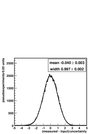
Figure 11: Pull distribution from pseudoexperiments run with the likelihood used to find the combined cross section.

IX.2 Pretag Sample

Using the event selection described in Section IV, we find 129 pretag candidate events in the data, which has an acceptance-weighted integrated luminosity of 1070 $\pm$ 60 pb^-1. The background is calculated to be 53.8 $\pm$ 6.7 events and the summed acceptance times efficiency is 0.84 $\pm$ 0.03%. Using these, we calculate the cross section using the likelihood fit described earlier in this section. Assuming $m_{t}=175$ $\mathrm{Ge\kern-1.00006ptV}/c^{2}$ and $BR(W\rightarrow\ell\nu)=10.8$ %, we find

$$\sigma_{t\overline{t}}=8.3\pm 1.3(\textrm{stat.})\pm 0.8(\textrm{sys.})\pm 0.5(\textrm{lum.})\ \textrm{pb ,}$$

consistent with the standard model prediction of $6.6^{+0.3}_{-0.5}$ (scale) ${}^{+0.4}_{-0.3}$ (PDF) pb Cacciari et al. (2008).

For the pretag sample, the signal and background predictions are summarized and compared to the observed number of candidate events, for events with zero, one, and two or more jets, in Table 11. The zero and one jet event comparisons test the background predictions, because the contribution from $t\bar{t}$ in these jet multiplicities is very small. The number of events predicted and observed agree for all jet multiplicities, although it should be noted that the zero jet events are not as strong of a cross-check, since a subset of these is used to derive the opposite-sign fraction for $W$ + jets events with a fake lepton (see Section VII.1). Figure 12 is a visual representation of Table 11. In both the table and the figure, the signal prediction is shown at the theoretical cross section value of 6.7 pb, but the backgrounds which depend on the $t\bar{t}$ cross section are calculated at the measured value of 8.3 pb.

	0 jets			1 jet			$\geq 2$ jets
$WW$	85.8 $\pm$	8.	7	14.9 $\pm$	1.	5	3.7 $\pm$	0.	4
$WZ$	9.3 $\pm$	1.	0	4.3 $\pm$	0.	5	1.3 $\pm$	0.	2
$ZZ$	6.0 $\pm$	0.	6	1.6 $\pm$	0.	2	0.8 $\pm$	0.	1
$Z/\gamma^{\star}\rightarrow ee$	71.3 $\pm$	15.	7	25.5 $\pm$	6.	0	7.6 $\pm$	2.	2
$Z/\gamma^{\star}\rightarrow\mu\mu$	17.9 $\pm$	5.	2	8.4 $\pm$	2.	7	3.2 $\pm$	1.	1
$Z/\gamma^{\star}\rightarrow\tau\tau$	35.5 $\pm$	3.	2	26.5 $\pm$	2.	5	7.3 $\pm$	0.	9
Fakes	244.1 $\pm$	46.	4	76.8 $\pm$	14.	6	29.9 $\pm$	5.	9
All Backgrounds	469.9 $\pm$	52.	5	157.9 $\pm$	17.	2	53.8 $\pm$	6.	7
$t\bar{t},\sigma=6.7$ pb	1.2 $\pm$	0.	1	17.3 $\pm$	0.	6	60.3 $\pm$	1.	9
Predicted	471.1 $\pm$	52.	5	175.2 $\pm$	17.	3	114.2 $\pm$	7.	1
Observed	443			187			129

Table 11: Predicted and observed pretag events in 1.1 fb^-1, with details of the background contributions. Systematic uncertainties on the predictions are included.

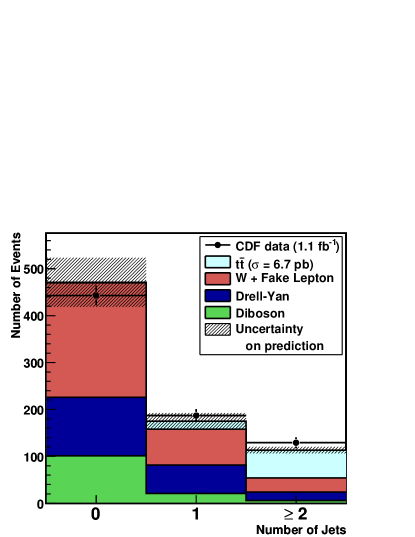
Figure 12: Number of predicted pretag lepton + track events compared to the number observed in the CDF data. The cross-hatched areas show the combined statistical and systematic uncertainties (one standard deviation) on the prediction.

The cross section calculated at other values of $m_{t}$ is shown in Table 14. The measured cross section decreases with increasing $m_{t}$ even though the number of observed events is unchanged. For higher top quark masses $t\bar{t}$ decay products are more energetic and therefore more likely to pass the kinematic selection, increasing the acceptance. The background estimates also depend weakly on the top quark mass through the use of simulated $t\bar{t}$ events to calculate the prevalence of $t\bar{t}$ in control data samples and the background from $t\bar{t}$ lepton + jets events with a fake lepton.

We compare the kinematic features of the observed pretag lepton + track candidates to the expected distributions. In each of these figures, the $t\bar{t}$ contribution is normalized to the measured cross section, so only the shapes of the distributions are to be compared, not the normalization. One of the most prominent features of dilepton $t\bar{t}$ events in particular is the ${\not\!\!E_{T}}$ from the two neutrinos. Figure 13 compares the ${\not\!\!E_{T}}$ spectrum of candidate events to the summed spectra expected for signal and background as predicted by simulation. Because the top quark is so massive, the $H_{T}$ distribution of $t\bar{t}$ events, defined as the scalar sum of the primary lepton $E_{T}$, track lepton $p_{T}$, ${\not\!\!E_{T}}$, and the $E_{T}$ of all jets in the event, is also distinctive. The $H_{T}$ distribution, shown in Fig. 14, is skewed toward higher values for the $t\bar{t}$ signal than for its backgrounds. Turning to the charged leptons in the event, we show the $p_{T}$ of the fully reconstructed lepton and the track lepton in Fig. 15, and their invariant mass in Fig. 16. Fig. 15 is useful for comparing the signal to the background contribution from events with a fake lepton, since the latter produces a much softer lepton $p_{T}$ distribution, due to the exponentially falling jet $p_{T}$ spectrum. Similarly, Fig. 16 is useful for comparing the signal to the background from Drell-Yan events, since the invariant mass distribution is more peaked for this background than for the signal. The agreement between the predicted and observed distributions suggests that the content of the candidate sample is well-understood within the uncertainties.

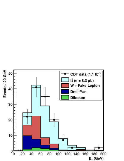
Figure 13: Missing transverse energy of pretag lepton + track candidate events with two or more jets, compared to the predicted distribution. The highest bin shown includes all events which would be past the right edge of the plot.

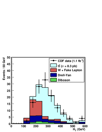
Figure 14: Summed transverse energy ($H_{T}$) of pretag lepton + track candidate events with two or more jets, compared to the predicted distribution. The sum includes the fully reconstructed lepton, the track lepton, the ${\not\!\!E_{T}}$, and all jets passing the analysis selection. The highest bin shown includes all events which would be past the right edge of the plot.

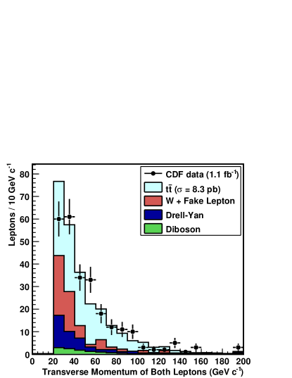
Figure 15: Distribution of lepton transverse momenta in pretag lepton + track candidate events with two or more jets, compared to the predicted distribution. There are two entries for each event; one each for the fully reconstructed lepton and the isolated track. For fully reconstructed electrons, the $E_{T}$ is used to estimate the $p_{T}$. The highest bin shown includes all events which would be past the right edge of the plot.

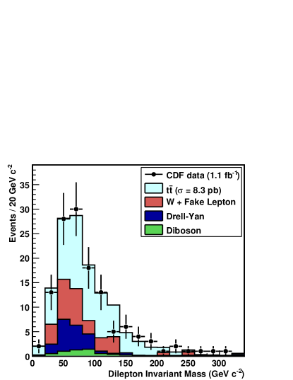
Figure 16: Reconstructed invariant mass of the fully reconstructed lepton and isolated track pair in pretag candidate events with two or more jets, compared to the predicted distribution. The highest bin shown includes all events which would be past the right edge of the plot.

IX.3 Tagged Sample

In the tagged sample, we find 69 candidate events, and measure 9.5 $\pm$ 2.8 background events. The predicted and observed numbers of events in the sample, with the prediction divided by source, are shown in Table 12. The inputs to the tagged cross section calculation are summarized in Table 13. Using data with an integrated luminosity of 1000 $\pm$ 60 pb^-1, and assuming $m_{t}=175$ $\mathrm{Ge\kern-1.00006ptV}/c^{2}$ and $BR(W\rightarrow\ell\nu)=10.8$ % we find:

$$\sigma_{t\overline{t}}=10.5\,^{+1.4}_{-1.3}\;(\textrm{stat.})\;^{+0.8}_{-0.7}\;(\textrm{sys.})\pm 0.6(\textrm{lum.})\ \textrm{pb .}$$

The tagged cross section as a function of assumed top quark mass is included in Table 14. Similar to the pretag measurement, the background estimate is relatively insensitive to the value of the top quark mass. The event tagging efficiency, for top quark masses between 170 and 180 $\mathrm{Ge\kern-1.00006ptV}/c^{2}$, is consistent with that measured at $m_{t}$ = 175 $\mathrm{Ge\kern-1.00006ptV}/c^{2}$. Therefore, the only change to the measurement as a function of the top quark mass is the acceptance for $t\bar{t}$ events.

The tagged cross section has a combined lower uncertainty of 1.6 pb, including the uncertainty on the luminosity. This translates to an excess above the standard model prediction of 2.4 in units of the calculated uncertainty on the measurement. However, the tagged measurement is consistent with the pretag measurement. The two measurements differ by the observed 2.2 pb in about 10% of pseudoexperiments, where the exact fraction depends on the assumed true cross section. The kinematic features of the observed candidates are also consistent with the standard model expectation, which for the tagged sample are predominantly $t\bar{t}$.

Figures 17-21 display some of the kinematic features of the tagged candidate sample, compared the expected combined signal and background contribution. In all of these figures, the signal is normalized to the measured cross section. The $H_{T}$ and ${\not\!\!E_{T}}$ of the tagged candidate events are shown in Fig. 17 and Fig. 18, respectively. These both have distinctive distributions for $t\bar{t}$ events; see the discussion above on pretag kinematic distributions for details. Fig. 19 and 20 show the transverse momentum distributions of the fully reconstructed leptons and the isolated tracks. Fig. 21 shows a unique feature of the tagged events, the distance along the tagged jet axis from the interaction point to the reconstructed secondary vertex, which corresponds to the distance traveled by the $b$ hadron before decaying. In all of the figures, the last bin on the right includes all events which would be past the right edge of the plot.

In all of the distributions, good agreement is observed between the candidate events from data and the expected distributions. Comparing the distributions from the tagged sample to the ones from the pretag sample, the improvement in sample purity from the $b$-tag requirement is evident. The agreement between the predicted and observed distributions shows that although the measured cross section is on the high side, the observed candidates are consistent with the expected $t\bar{t}$ signature.

Source	Number of events
From Matrix (e.g. $Z+b\bar{b}$)	4.4 $\pm$	2.6
Fakes	5.2 $\pm$	1.2
All Backgrounds	9.5 $\pm$	2.8
$t\bar{t},\sigma=6.7$ pb	37.7 $\pm$	2.4
Predicted	47.3 $\pm$	3.7
Observed	69

Table 12: Predicted and observed events with two or more jets, at least one of which is tagged, in 1.0 fb^-1, with details of the background contributions.

Input	Value
$N^{\textrm{\tiny{tag}}}$	69
$N^{\textrm{\tiny{tag}}}_{\textrm{\tiny{bkgd}}}$	9.	5 $\pm$	2.8
$\mathcal{A}\times\int\mathscr{L}dt$	8.	4 $\pm$	0.03 pb-1
$\epsilon_{\textrm{\tiny{tag}}}$	0.	669 $\pm$	0.037

Table 13: Predicted background and observed events in 1.0 fb^-1, with inputs to the cross section calculation for the tagged analysis. Systematic uncertainties are included in the prediction numbers.

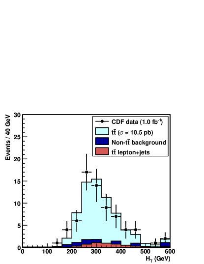
Figure 17: Summed scalar energy ($H_{T}$) of the fully reconstructed lepton, the isolated track, the ${\not\!\!E_{T}}$ and all jets in the tagged candidate sample, compared to the combined signal and background predictions.

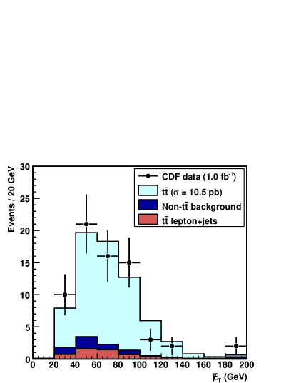
Figure 18: Missing transverse energy of the lepton + track tagged candidate sample, compared to the combined signal and background predictions.

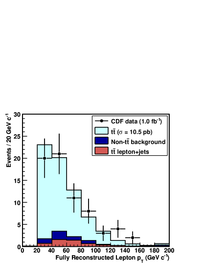
Figure 19: Transverse momentum of the fully reconstructed lepton in the tagged lepton + track candidate sample, compared to the combined signal and background predictions. The $E_{T}$ is used as an estimate of the lepton $p_{T}$ for fully reconstructed electron candidates.

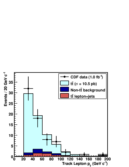
Figure 20: Transverse momentum of the track lepton (isolated track) in the tagged lepton + track candidate sample, compared to the combined signal and background predictions.

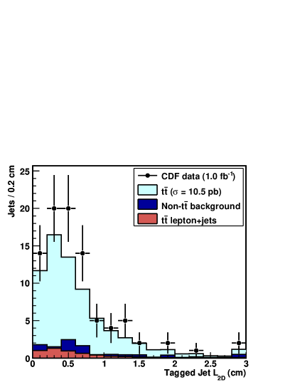
Figure 21: Distance along the jet axis to the reconstructed secondary vertex in tagged jets in the lepton + track candidate sample, compared to the combined signal and background predictions.

IX.4 Combined Cross Section Results

Using the likelihood fitter, we find a combined cross section of

$$\sigma_{t\bar{t}}=9.6_{-1.3}^{+1.4}(\textrm{stat+sys})\pm 0.6(\textrm{lum})\ \textrm{pb }$$

or

$$\sigma_{t\bar{t}}=9.6\pm 1.2(\textrm{stat})_{-0.5}^{+0.6}(\textrm{sys})\pm 0.6(\textrm{lum})\ \textrm{pb.}$$

The 14% combined statistical and systematic uncertainty is an improvement in precision on either of the individual measurements. The combined cross section is also shown as a function of the assumed top quark mass in Table 14 and Fig. 22. In both, the measured cross section is compared to the theoretical prediction. Both the predicted and measured cross section depend on the top quark mass, but the dependence is stronger for the predicted cross section. The predicted cross section drops off with increasing top quark mass because of the increased collision energy needed to exceed the kinematic threshold for pair production of top quarks. The measured cross section depends on the assumed mass more weakly, through the increased acceptance at higher top quark masses because of the increased average transverse momentum of the decay products.

To facilitate comparison of this result with other measurements and calculations, which may be performed at different assumed top quark masses, we fit the combined cross section results shown in Table 14 to the functional form

$$\sigma_{t\bar{t}}(m_{t})=A+B(m_{t}-175)+C(M_{t}-175)^{2}\ \textrm{,}$$

in the spirit of Ref. Cacciari et al. (2008). The top quark mass $m_{t}$ is in $\mathrm{Ge\kern-1.00006ptV}/c^{2}$, and the fit yields the coefficients $A=9.6$ pb, $B=4.4\times 10^{-2}$ pb/($\mathrm{Ge\kern-1.00006ptV}/c^{2}$), and $C=9.6\times 10^{-3}$ pb/($\mathrm{Ge\kern-1.00006ptV}/c^{2}$)².

We compare the measured cross section to the standard model prediction at the current world average measurement, 173.1 $\mathrm{Ge\kern-1.00006ptV}/c^{2}$ Tevatron Electroweak Working Group (2009). Using the fit described in the previous paragraph, we measure $9.7^{+1.5}_{-1.4}$ pb, where the uncertainty includes the statistical, systematic, and luminosity uncertainties. The prediction for this top quark mass from Ref. Cacciari et al. (2008) is $7.0^{+0.5}_{-0.6}$ pb. The uncertainty on the difference between the two, 1.5 pb, includes the uncertainty on the measurement and the theoretical prediction. The significance of the the difference is therefore $2.7\ \textrm{pb}/1.5\ \textrm{pb}=1.8$. Comparison of the kinematics of the pretag and tagged candidate samples to the standard model expectation shows that the content of the sample is reasonably well-understood. Also, the measurement agrees with the DØ measurement in the dilepton channel, $7.4\pm 1.4$ (stat.) $\pm 0.9$ (sys.) $\pm 0.5$ (lum.) pb Abazov et al. (2007a), as well as with the published measurements from other channels cited in the Introduction, most of which are also above the predicted theoretical value.

Input	Theoretical	Pretag	Measured cross section (pb)
$m_{t}$ ($\mathrm{Ge\kern-1.00006ptV}/c^{2}$)	$\sigma$ (pb)	$t\bar{t}$ Acceptance	Pretag		Tagged		Combined
170	$7.7_{-0.7}^{+0.6}$	0.80 $\pm$ 0.02 %	8.	8 ${}_{-1.6}^{+1.7}$	11.	0 ${}_{-1.5}^{+1.7}$	10.	1 ${}_{-1.3}^{+1.4}$
172.5	$7.1_{-0.6}^{+0.6}$	0.83 $\pm$ 0.02 %	8.	5 ${}_{-1.5}^{+1.7}$	10.	7 ${}_{-1.5}^{+1.7}$	9.	8 ${}_{-1.3}^{+1.4}$
175	$6.6_{-0.6}^{+0.5}$	0.84 $\pm$ 0.03 %	8.	3 ${}_{-1.5}^{+1.6}$	10.	5 ${}_{-1.5}^{+1.6}$	9.	6 ${}_{-1.3}^{+1.4}$

Table 14: The pretag and tagged cross section as calculated at several input top masses. Theoretical prediction from Ref. Cacciari et al. (2008). The statistical and systematic uncertainties are combined, and a common uncertainty of 6%, due to the uncertainty on the integrated luminosity, is omitted.

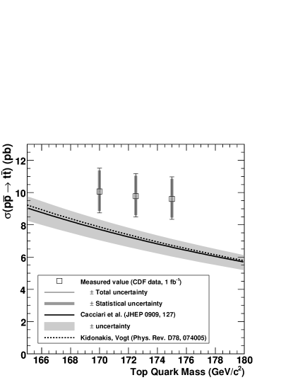
Figure 22: Measured cross section as a function of the assumed top quark mass, compared to theoretical predictions for the cross section.

X Conclusion

We have measured the $t\bar{t}$ production cross section in the dilepton channel using events selected with one fully reconstructed lepton and one isolated track, both with and without the requirement that at least one jet in the event be tagged as a $b$. The combined result of these measurements is

$$\sigma_{t\bar{t}}=9.6\pm 1.2(\textrm{stat})_{-0.5}^{+0.6}(\textrm{sys})\pm 0.6(\textrm{lum})\ \textrm{pb}$$

for a top quark mass of 175 $\mathrm{Ge\kern-1.00006ptV}/c^{2}$. This is the first dilepton cross section result from CDF which uses $b$-tagging information. We have also improved the estimation of the pretag backgrounds with respect to the previous publication, particularly for the background from events in which a jet has been reconstructed as an isolated track. These changes, combined with the integration of more data, result in a more precise measurement of the cross section in the dilepton channel compared to other published results.

The cross sections measured are high compared to the standard model prediction, but the consistency between the tagged and pretag measurements, their agreement with other published measurements, and the consistency of the candidate event kinematics with the standard model all support the hypothesis that the high cross sections observed are consistent with an upward fluctuation in the number of $t\bar{t}$ events accepted by the lepton + track selection.