Domain Walls and Double Bubbles

Abstract

We study configurations of intersecting domain walls in a Wess-Zumino model with three vacua. We introduce a volume-preserving flow and show that its static solutions are configurations of intersecting domain walls that form double bubbles, that is, minimal area surfaces which enclose and separate two prescribed volumes. To illustrate this field theory approach to double bubbles, we use domain walls to reconstruct the phase diagram for double bubbles in the flat square two-torus and also construct all known examples of double bubbles in the flat cubic three-torus.

1 Introduction

Kinks are examples of topological solitons (for a review see [8]) in one space dimension, which interpolate between distinct vacua. A kink can be trivially embedded into three-dimensional Euclidean space as a solution which is independent of all but one spatial direction, and this is known as a domain wall. The energy of a domain wall is proportional to its surface area, therefore the embedding into $\hbox{\mybb R}^{3}$ gives a domain wall with infinite energy. However, the domain wall does have finite energy per unit area, which is the tension of the wall, and is equal to the kink energy in the one-dimensional theory.

Domain walls can be constructed in a three-dimensional compact space, in which case they have finite energy. A minimal energy configuration of domain walls approximates a minimal surface with increasing accuracy as the thickness of the domain wall is reduced. The surface associated with a configuration of domain walls can equivalently be defined as the level set of the field (taking the level set value to be the midpoint between the two vacua) or as a maximal energy density isosurface. This approach of modelling minimal surfaces using domain walls has been successfully implemented numerically to investigate both triply periodic and quasicrystalline minimal surfaces [5, 11].

In this paper, we extend the domain wall description of minimal surfaces to double bubbles, which are global minimal area surfaces which enclose and separate two prescribed volumes. We show that intersecting domain walls in a Wess-Zumino theory with three vacua form double bubbles under a certain volume-preserving flow.

In 2002 it was proved [7] that in three-dimensional Euclidean space the double bubble consists of three segments of round spheres, with radii $R_{1}\leq R_{2}\leq R_{3},$ satisfying the relation $R_{1}^{-1}=R_{2}^{-1}+R_{3}^{-1},$ and meeting in triple junctions at angles of $120^{\circ}.$ Such a configuration is known as the standard double bubble and is the familiar structure seen in soap bubbles. The proof [7] followed an earlier computer assisted proof [6], restricted to the situation in which the two prescribed volumes are equal.

On compact spaces the double bubble problem is far more complicated. Even in the flat cubic three-torus, it is still an open problem to prove the form taken by a double bubble. The only rigorous result is that the standard double bubble is recovered if the size of the double bubble is sufficiently small compared to the size of the torus [2]. Numerical investigations have been performed for the flat cubic three-torus [2] using Brakke’s surface evolver software [1], which is based on adaptive computations of triangulations of the surface. These numerical results suggest ten different qualitative forms taken by the double bubble, depending upon the two bubble volumes relative to the volume of the torus.

In two space dimensions the double bubble problem is better understood, and consists of determining the curve with minimal perimeter that encloses and separates two prescribed areas. Note that in the two-dimensional case the term volume will often be used rather than area, in order to keep the terminology of the three-dimensional situation, but we shall always refer to perimeter as the quantity to be minimized. In the flat square two-torus it has been proved [3] that the double bubble takes one of four different qualitative forms, and explicit formulae are available for the perimeter of each form as a function of the two bubble volumes. A numerical evaluation of these formulae then allows the determination of the form of the double bubble for any given pair of bubble volumes, and hence the construction of a phase diagram.

To illustrate the applicability of our domain wall approach to double bubbles we reconstruct the phase diagram for double bubbles in the flat square two-torus and also construct all known examples of double bubbles in the flat cubic three-torus.

2 Domain walls in the Wess-Zumino model

The field theory of interest in this paper is the bosonic sector of the Wess-Zumino model, which contains a single complex scalar field $\phi.$ For static fields the theory may be defined by its energy density, which is given by

$${\cal E}=\frac{1}{4}\partial_{i}\phi\partial_{i}\bar{\phi}+\left|\frac{dW}{d\phi}\right|^{2},$$ (2.1)

where $W(\phi)$ is the superpotential. For applications to double bubbles we require a triply degenerate vacuum and therefore take the superpotential to be

$$W=\phi-\frac{1}{4}\phi^{4}.$$ (2.2)

The zero energy vacuum field configurations are the three cube roots of unity $\phi=\omega^{j}\equiv\phi_{j},$ where $\omega=e^{i2\pi/3},$ with $j\in\{1,2,3\}.$

In one space dimension this theory has six types of kink solutions (including anti-kinks, as we make no distinction between these in this paper), which are the minimal energy field configurations $\phi(x)$ that interpolate between any two distinct vacua, that is, $\phi(-\infty)=\phi_{i}$ and $\phi(+\infty)=\phi_{j},$ with $i\neq j.$ These kinks satisfy a first-order Bogomolny equation and have an energy given by

$$E=\int^{\infty}_{-\infty}{\cal E}\,dx=|W(\phi_{i})-W(\phi_{j})|=3\sqrt{3}/4.$$ (2.3)

Kinks in the above theory have a width of order one, but introducing a constant $\epsilon^{2}$ in front of the first term in (2.1) makes the kink width $O(\epsilon).$ The thin wall limit is $\epsilon\rightarrow 0,$ and rigorous results require proofs based on regularity as this limit is approached. However, as only relative scales are relevant, we find it more convenient for a numerical implementation to fix the kink scale to be of order one and consider all other scales in the problem (such as the size of a region containing a single vacuum) to be $O(\epsilon^{-1}).$

A trivial embedding of kinks into a higher-dimensional version of the theory (two and three spatial dimensions will be considered) yields domain walls with tension $\mu=3\sqrt{3}/4.$ The tension is simply the energy per unit area in three dimensions and the energy per unit length in two dimensions.

A kink traces out a curved path in the $\phi$-plane, connecting two distinct vacua, but it can be shown that when viewed in the $W$-plane the path is simply a straight line [4]. We will make use of this fact later.

This theory has a domain wall junction [4], which also satisfies a first-order Bogomolny equation, in which the three types of domain wall mutually intersect at angles of $120^{\circ}$, dividing space into three equal sectors with a different vacuum value occuring in the interior of each sector. The junction has $120^{\circ}$ angles because all domain walls have the same tension and there must be a tension balance for an equilibrium configuration. The domain wall junction has been computed numerically, together with networks of junctions connected by domain wall segments that yield tilings of the plane [10].

The salient features are that the energy of a domain wall is proportional to its surface area, and three intersecting domain walls form a junction with $120^{\circ}$ angles. These properties suggest that domain walls in this system may provide a useful field theory description of double bubbles.

3 A volume-preserving flow

A bubble configuration in three dimensions consists of a spherical domain wall separating one vacuum field in the interior of the bubble from a distinct vacuum field in the exterior of the bubble. The energy of such a bubble configuration is approximately $\mu A$, where $A$ is the surface area of the bubble and $\mu$ is the tension introduced above. The error in this approximation can be made arbitrarily small by increasing the ratio of the bubble radius to the width of the domain wall, that is, by approaching the thin wall limit. Clearly, for the energy density (2.1), there are no bubbles that are stationary points of the energy. In order to have a bubble (and later double bubbles) a constraint on the volume of the bubble must be included within the field theory description, since in this theory there is no pressure to resist the tension-induced collapse. In the following we describe how volume constraints may be included in a natural manner within the field theory.

There are two obvious ways in which dynamics may be introduced into the static theory discussed in the previous Section. The first is to consider relativistic dynamics, which leads to the usual Lagrangian description of the Wess-Zumino model and yields a nonlinear wave equation which is second-order in the time derivative. The other obvious dynamics is gradient flow, which produces a nonlinear diffusion equation that is first-order in time and generates an energy decreasing evolution. Given the above discussion, it is easy to see that in both cases an initial bubble configuration will simply collapse, as this reduces the potential energy.

In the real Ginzburg-Landau model, it is known that gradient flow dynamics can be modified by the introduction of a time-dependent effective magnetic field that preserves the global average of the field. This volume-preserving flow is used, for example, in the study of phase ordering and interface-controlled coarsening [9]. In this Section we describe a generalization of this volume-preserving flow which is applicable to the Wess-Zumino model and allows two independent volumes to be preserved during the flow.

Motivated by the applications to follow, we consider the theory defined on a torus $T^{d},$ with volume $V.$

First of all, for each vacuum we need to introduce a density function, such that it is equal to unity if the field is in the given vacuum and vanishes if the field is in any other vacuum. A simple choice is

$$v_{i}(\phi)=\frac{|\phi-\phi_{j}|^{2}|\phi-\phi_{k}|^{2}}{|\phi_{i}-\phi_{j}|^{2}|\phi_{i}-\phi_{k}|^{2}}=\frac{1}{9}|\phi-\phi_{j}|^{2}|\phi-\phi_{k}|^{2},$$ (3.1)

where $i,j,k$ are three distinct elements of $\{1,2,3\}.$ Clearly these functions satisfy the required property that $v_{i}(\phi_{j})=\delta_{ij}.$ Next we define the volume occupied by each vacuum as

$$V_{i}=\int_{T^{d}}v_{i}\,d^{d}x.$$ (3.2)

In the thin wall limit, the width of the domain wall is negligible compared to the volumes occupied by the vacua, and therefore in this limit $V_{1}+V_{2}+V_{3}\rightarrow V.$

The task is to construct an energy minimizing gradient flow in which both volumes $V_{1}$ and $V_{2}$ remain constant. Note that $V_{3}$ is then automatically constant, at least to the accuracy in which the thin wall limit is approached, as $V_{3}=V-V_{1}-V_{2}.$

The starting point is the gradient flow dynamics associated with the energy density (2.1)

$$\frac{\partial\phi}{\partial t_{0}}=-\frac{\delta{\cal E}}{\delta\bar{\phi}}\equiv F=\frac{1}{4}\partial_{i}\partial_{i}\phi+3(1-\phi^{3})\bar{\phi}^{2}.$$ (3.3)

The dynamics that follows from flow in the $t_{0}$ time variable reduces the energy $E$ but also changes the volumes $V_{i}.$

Associated with each volume density $v_{i}$ one can define an alternative gradient flow

$$\frac{\partial\phi}{\partial t_{i}}=-\frac{\partial v_{i}}{\partial\bar{\phi}}\equiv f_{i}=\frac{1}{9}(\phi-\phi_{j})(\phi-\phi_{k})(2\bar{\phi}-\bar{\phi}_{j}-\bar{\phi}_{k}),$$ (3.4)

so that evolution in the time variable $t_{i}$ is a flow that reduces the volume $V_{i}.$

The idea is to introduce a new flow, with time variable $t,$ that is constructed from the $t_{0}$ flow by projecting out the components in the directions of the $t_{i}$ flows. This makes the $t$ flow orthogonal to all $t_{i}$ flows and hence preserves all the volumes $V_{i}.$

The appropriate inner product is

$$<f,g>\,=\frac{1}{V}\int_{T^{d}}\bar{f}g\,d^{d}x,$$ (3.5)

and we use the notation

$$||f||=\sqrt{<f,f>}.$$ (3.6)

Given the flows (3.4) an orthonormal set of flows $\widehat{f}_{i}$ is constructed as

$$\widetilde{f}_{i}=f_{i}-\sum_{j<i}<\widehat{f}_{j},f_{i}>\widehat{f}_{j},\quad\mbox{then}\quad\widehat{f}_{i}=\frac{\widetilde{f}_{i}}{||\widetilde{f}_{i}||}.$$ (3.7)

Finally, the $t$ flow is defined to be

$$\frac{\partial\phi}{\partial t}=F-\sum_{i=1}^{2}<\widehat{f}_{i},F>\widehat{f}_{i},$$ (3.8)

which is a nonlocal and nonlinear reaction diffusion equation. By construction the flow (3.8) is orthogonal to all the $t_{i}$ flows, that is,

$$<f_{i},\frac{\partial\phi}{\partial t}>\,=0.$$ (3.9)

It is easy to prove that the flow (3.8) preserves both volumes $V_{i},$ with $i=1,2$, while reducing the energy $E.$ First of all,

$$\frac{dV_{i}}{dt}=\int_{T^{d}}\frac{dv_{i}}{dt}\,d^{d}x=2\Re\int_{T^{d}}\frac{\partial v_{i}}{\partial\phi}\frac{\partial\phi}{\partial t}\,d^{d}x=-2\Re\int_{T^{d}}\bar{f}_{i}\frac{\partial\phi}{\partial t}\,d^{d}x=-2V\Re<f_{i},\frac{\partial\phi}{\partial t}>\,=0,$$ (3.10)

where we have used the orthogonality property (3.9).

To prove that the flow is energy decreasing, it is convenient to write the sum in (3.8) as a single term, by defining

$$\widehat{f}=\frac{<\widehat{f}_{1},F>\widehat{f}_{1}+<\widehat{f}_{2},F>\widehat{f}_{2}}{\sqrt{<\widehat{f}_{1},F>^{2}+<\widehat{f}_{2},F>^{2}}}.$$ (3.11)

Using the orthogonality property $<\widehat{f}_{1},\widehat{f}_{2}>=0,$ allows (3.8) to be rewritten as

$$\frac{\partial\phi}{\partial t}=F-<\widehat{f},F>\widehat{f}.$$ (3.12)

Therefore,

$$\frac{dE}{dt}=\int_{T^{d}}\frac{d{\cal E}}{dt}\,d^{d}x=2\Re\int_{T^{d}}\frac{\partial\bar{\phi}}{\partial t}\frac{\delta{\cal E}}{\delta\bar{\phi}}\,d^{d}x=-2\Re\int_{T^{d}}\frac{\partial\bar{\phi}}{\partial t}F\,d^{d}x=-2V\Re<\frac{\partial\phi}{\partial t},F>$$

$$=-2V\Re<\frac{\partial\phi}{\partial t},\frac{\partial\phi}{\partial t}+<\widehat{f},F>\widehat{f}>=-2V\Re<\frac{\partial\phi}{\partial t},\frac{\partial\phi}{\partial t}>\,\,\leq 0,$$ (3.13)

where the last expression uses the fact that the $t$ flow is perpendicular to the combined volume reducing flow, that is, $<\frac{\partial\phi}{\partial t},\widehat{f}>\,=0.$

In summary, we have proved that the flow (3.8) is energy decreasing while preserving both volumes $V_{1}$ and $V_{2}.$ The end points of this flow are therefore equilibrium configurations that are critical points of the energy functional under constrained variations that preserve both volumes. Static solutions of this flow are candidates for double bubbles.

The volume-preserving flow of the real Ginzburg-Landau model is recovered from the above generalization by restricting $\phi$ to be real $\phi=\bar{\phi}\equiv\varphi$ and choosing the volume density to be $v_{1}=(\varphi-\varphi_{2})/(\varphi_{1}-\varphi_{2}),$ where $\varphi_{1}$ and $\varphi_{2}=-\varphi_{1}$ are the two real vacua. In this case $f_{1}=1$ and the flow takes the form

$$\frac{\partial\varphi}{\partial t}=F-<F>,$$ (3.14)

where $<F>\,\equiv\,<1,F>$ is the average value of $F$. This flow clearly preserves the average volume as $\frac{\partial}{\partial t}<\varphi>=0.$

The definition of a double bubble requires the surface to be the global minimum of the area functional, with the prescribed volume constraints. Therefore, there may be a number of surfaces which are local minima of the surface area, or even saddle points, but are not double bubbles. All local minima must be found to determine which is the double bubble, and this applies to the field theory energy computations too.

In the following two Sections we present the results of a numerical implementation of the above volume-preserving flow. Double bubbles in the two-torus and three-torus are studied and comparisons made with previous results obtained using other methods that are not based on field theory.

4 Double bubbles in the two-torus

In this Section we restrict our investigations to two-dimensional double bubbles. As mentioned earlier, we shall retain the three-dimensional notation and refer to the volume of a bubble (even though it is an area). The problem is to find curves with minimal perimeter that enclose and separate two prescribed volumes.

Although we work on the flat square two-torus, the case of the Euclidean plane can be recovered if the torus is sufficiently large, so that no curve of the double bubble wraps a cycle of the torus. As a first illustration of our method, we discuss an example of this type.

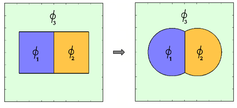
Figure 1: The image on the left shows the initial condition and the image on the right is the subsequent final field configuration obtained under the volume-preserving flow. Different colours (or shades of grey) represent regions in space where the field takes values in one of the three different vacua $\phi_{1},\phi_{2},\phi_{3}.$ Lines denote the domain wall positions.

Figure 1 presents an initial condition and the subsequent final field configuration obtained under the volume-preserving flow. The lattice contains $401^{2}$ grid points with a lattice spacing $\Delta x=0.2$ so that the volume of the torus is $V=6400.$ The Laplacian is evaluated using second-order accurate finite difference approximations and the flow is evolved using a simple first-order accurate explicit method with timestep $\Delta t=0.008.$ All inner products are evaluated by approximating the integral by a sum over lattice sites.

The initial condition in Figure 1 consists of two equal volume rectangles, each of volume $V_{1}=V_{2}=0.15V,$ with the field set to the vacuum value $\phi_{1}$ inside one rectangle and $\phi_{2}$ inside the other rectangle. Outside these rectangles the field takes the value $\phi_{3}.$ The final configuration shown is at time $t=400,$ when the field is static to the accuracy that we compute. The equilibrium field configuration clearly takes the form of the standard double bubble in the plane with equal volumes. Note the $120^{\circ}$ intersection angles of the domian wall junctions.

The perimeter, $P,$ of a standard double bubble in the plane with equal volumes $V_{1}=V_{2}$ satisfies [3]

$$\frac{P}{\sqrt{V_{1}}}=\frac{16\pi+6\sqrt{3}}{\sqrt{24\pi+9\sqrt{3}}}=6.359\ldots$$ (4.1)

Computing the perimeter length in the field theory, as the ratio of the energy to the tension $E/\mu,$ gives the result

$$\frac{E}{\mu\sqrt{V_{1}}}=6.370$$ (4.2)

therefore the field theory computation has an error of less than $\frac{1}{4}\%$ for this choice of simulation parameters, which has quite a modest grid. The accuracy can be improved by increasing the number of grid points, so that the size of the torus $\sqrt{V}$ increases relative to the width of the domain wall, that is, the system is moved closer to the thin wall limit. In Section 6 we discuss some modifications that can be applied to improve the accuracy of the computations without the need to increase the grid size.

Note that from now on we shall refer to all volumes in units of the torus volume, so for the above example we simply write $V_{1}=0.15,$ etc.

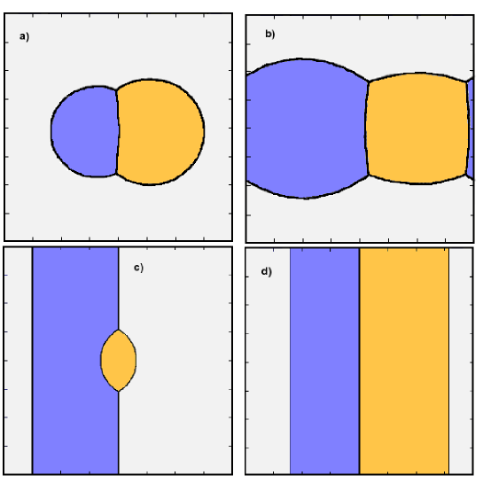
Figure 2: Equilibrium fields obtained from four different simulations with varying volumes. Different colours (or shades of grey) represent regions in space where the field takes values in one of the three different vacua. The configurations shown are known as (a) the standard double bubble, (b) the standard chain, (c) the band lens, (d) the double band.

Figure 2 presents equilibrium fields obtained from four different simulations with volumes $\{V_{1},V_{2}\}$ given by (a) $\{0.1,0.15\}$; (b) $\{0.3,0.2\}$; (c) $\{0.35,0.05\}$; (d) $\{0.3,0.4\}$. In each case the initial field consists of rectangular regions of vacuum, similar to that shown in Figure 2, though some of the rectangles were chosen to wrap the torus. In each case, for the chosen volumes, the resulting field configuration provides a good description of the double bubble. The configurations shown are known as (a) the standard double bubble, (b) the standard chain, (c) the band lens, (d) the double band. It has been proved that for all volumes $\{V_{1},V_{2}\}$ the double bubble takes one of these four forms, and a phase diagram has been computed to determine which of the four forms is taken for any given volumes [3].

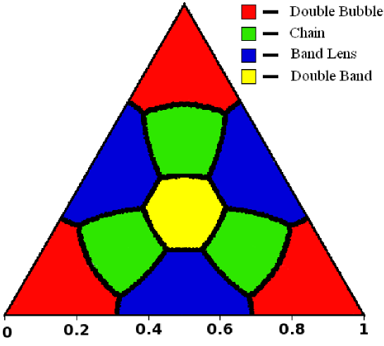
Figure 3: A phase diagram indicating the form taken by the double bubble as a function of the individual bubble volumes. A position of a point inside the triangle is related to the bubble volumes through equation (4.3). The centroid of the triangle is where all three volumes are equal, whereas regions near the vertices are where two volumes are much smaller than the third. Finally, one of the volumes vanishes at an edge, where the included scale gives the fraction of the total volume occupied by one of the two remaining volumes.

Using the field theory description we have been able to reproduce this phase diagram by performing simulations for a range of volumes. This phase diagram is presented in Figure 3. The set of possible volumes, $V_{1},V_{2},V_{3},$ such that $V_{1}+V_{2}+V_{3}=1,$ is represented by the interior of an equilateral triangle. Explicitly, the $(x,y)$ coordinates in the plane containing the triangle are related to the volumes by

$$(x,y)=\left(\frac{1}{2}(V_{1}-V_{2}),\frac{1}{2\sqrt{3}}(2-3V_{1}-3V_{2})\right).$$ (4.3)

The centroid of the triangle is $(x,y)=(0,0)$ and corresponds to $V_{1}=V_{2}=V_{3}=\frac{1}{3},$ so that all three volumes (including the volume exterior to both bubbles) are equal. In this case, both bubble volumes are large and therefore it is favourable to wrap both bubbles around the torus, as this reduces perimeter length, resulting in the double band. Note that the double bubble problem is symmetric under the interchange of any two of the three volumes, therefore the computation can be restricted to the region $V_{3}\geq V_{2}\geq V_{1},$ and the remainder of the phase diagram constructed from this sixth of the triangle by symmetry.

The regions near the vertices of the triangle correspond to the situation in which two volumes are much smaller than the third, and therefore the standard double bubble is recovered. The edges of the triangle are where one of the volumes vanishes, with the mid-point of an edge associated with the two non-vanishing volumes being equal. In a region around the mid-point of an edge the band lens is the optimal form. Finally, if two volumes are reasonably similar in size, and not too small, then the double bubble takes the form of the chain. The phase diagram displayed in Figure 3 is in excellent agreement with the one presented in [3] and confirms the applicability of our field theory approach to double bubbles.

5 Double bubbles in the three-torus

In this Section we turn our attention to the more complicated problem of double bubbles on the flat cubic three-torus. In this case even the classification of the types of double bubble that exist is an open problem and only numerical results are available [2]. If both bubble volumes are small compared to the volume of the torus then the standard double bubble in three-dimensional Euclidean space is recovered. One also expects various three-dimensional analogues of the two-dimensional double bubbles discussed in the previous Section. Numerical investigations have been performed [2] using the surface evolver software [1] and yield a number of forms taken by double bubbles for approriate volumes. These results suggest that there are ten different forms taken by double bubbles. Equilibrium configurations were also found that do not appear to be double bubbles for any values of the volumes.

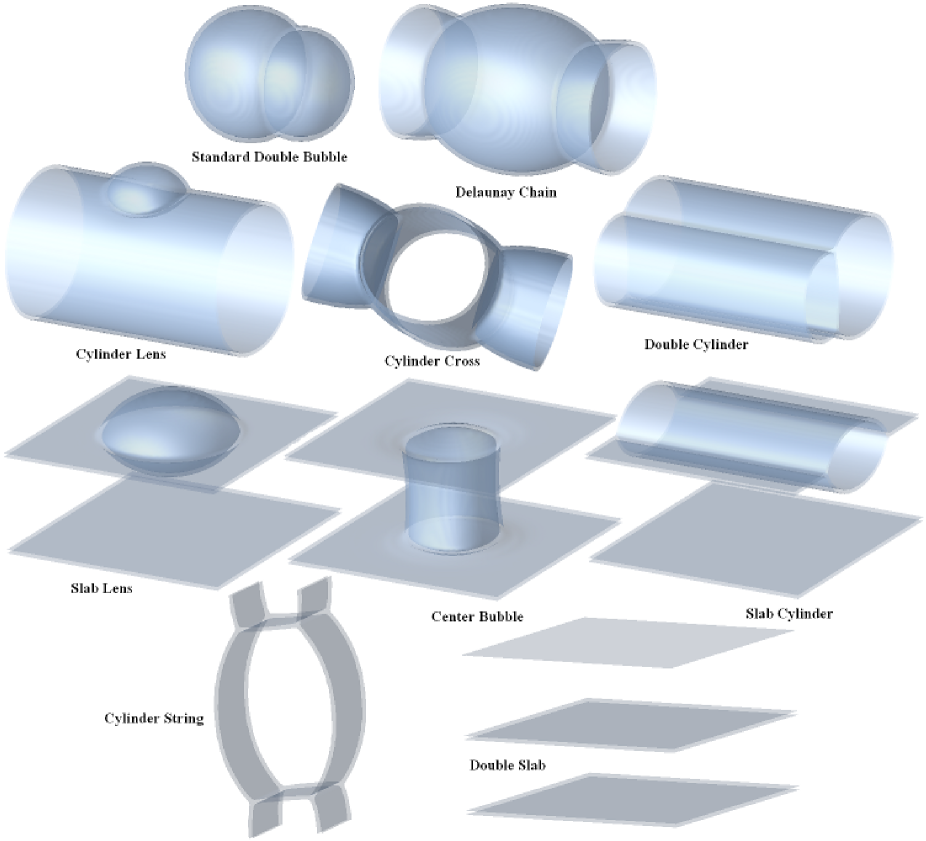
Figure 4: Energy density isosurfaces for equilibrium configurations corresponding to the ten different conjectured double bubble forms.

Using our field theory approach with domain walls, which we stress is very different to the surface triangulation method used in [2], we have been able to reproduce all ten types of equilibrium configurations conjectured to be doubles bubbles in [2]. In Figure 4 we display the ten different conjectured double bubble forms, by plotting an energy density isosurface for each, and we include the name of each surface using the nomenclature of [2].

The initial conditions used to generate these surfaces were constructed using the same approach as in the two-dimensional case described in the previous Section, namely, we take a collection of cuboids with assigned vacuum fields.

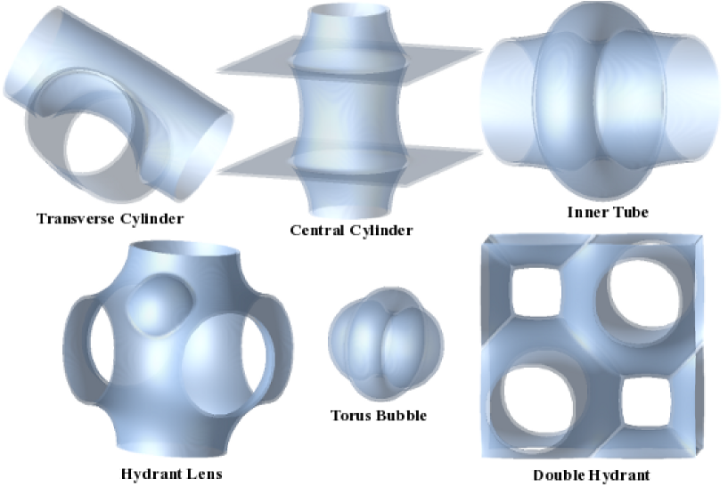
Figure 5: Energy density isosurfaces for six types of equilibrium configurations which are never double bubbles, that is, none is the global minimal energy surface for any values of the volumes.

Six types of equilibrium configurations are presented in Figure 5 which are never double bubbles, that is, none is the global minimal energy surface for any values of the volumes. The transverse cylinder, torus bubble, inner tube and double hydrant are saddle points which are unstable to symmetry breaking perturbations. The central cylinder and hydrant lens appear to be local minima, for suitable values of the volumes.

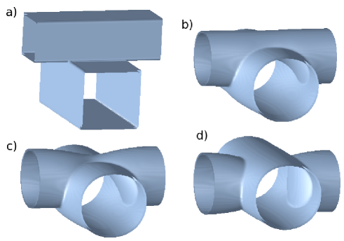
Figure 6: Energy density isosurfaces at increasing times under volume-preserving flow. The initial condition is of a similar type to the transverse cylinder but evolves into a cylinder cross.

An example evolution under volume-preserving flow is presented in Figure 6. The initial condition Figure 6(a) is of a similar type to the transverse cylinder, but under the evolution it evolves into a stable cylinder cross Figure 6(d). This simulation demonstrates both the instability of the transverse cylinder and the stability of the cylinder cross.

The results presented in this Section confirm the applicability of the domain wall approach to three-dimensional double bubbles and show that the method can be numerically realized with reasonable computing resources. Evolutions that involve topology changes of the surface are automatically dealt with within the field theory description, since the surface is obtained as a level set. This allows a large region of configuration space to be explored without the need for fine tuned initial conditions, as demonstrated in Figure 6, where the final equilibrium configuration is quite different from the initial condition. Our results provide some confirmation of the numerical results in [2] using very different methods, and therefore provides evidence for the accuracy of both approaches. The phase diagram for three-dimensional double bubbles computed in [2] could also be obtained using our field theory approach, though we have not pursued that here.

6 Modified volumes and penalty functions

In this Section we discuss an improvement on the simple volume density functions introduced earlier and also describe an alternative method to the volume-preserving flow.

The volume density functions (3.1) satisfy the minimal requirement that $v_{i}(\phi_{j})=\delta_{ij}.$ In the thin wall limit the volume of any region in which the field is not in a vacuum value tends to zero, so the above minimal requirement is all that is relevant. However, in any numerical implementation there is a non-zero value of the wall thickness (that is, $\epsilon\neq 0$), and the volume density (3.1) will provide a contribution to the volume as the domain wall is crossed. Considering the volume $V_{i}$ then the density will be non-zero in the interior of the domain wall connecting vacuum $\phi_{i}$ to $\phi_{j}.$ This is reasonable since the region containing vacuum $\phi_{i}$ now has a diffuse rather than sharp boundary. However, the simple volume density (3.1) is also non-zero in the interior of the domain wall connecting vacuum $\phi_{j}$ to $\phi_{k}$ and this is certainly not related to the volume $V_{i}.$ Of course, as the thin wall limit is approached this effect tends to zero, but from the point of view of improving numerical accuracy it would be desirable if this contribution could be eliminated for any wall thickness. This can be achieved using the modification presented below.

The above comments lead to an additional requirement on the volume density, namely that $v_{i}(\phi_{jk})=0,$ where $\phi_{jk}$ denotes the domain wall solution connecting vacuum $\phi_{j}$ to $\phi_{k}.$ Recall that although a domain wall solution traces out a curved path in the $\phi$-plane it is a straight line in the $W$-plane. The additional requirement can therefore be met by choosing a volume density $v_{i}(\phi)$ that vanishes along the whole line in the $W$-plane that connects the points $W(\phi_{j})$ and $W(\phi_{k}).$ The simplest choice is to take

$$v_{i}(\phi)=\bigg{(}\frac{\Im\{(W(\phi)-W(\phi_{k}))(\overline{W(\phi_{j})}-\overline{W(\phi_{k})})\}}{\Im\{(W(\phi_{i})-W(\phi_{k}))(\overline{W(\phi_{j})}-\overline{W(\phi_{k})})\}}\bigg{)}^{2},$$ (6.1)

which clearly satisfies the required properties.

We have used this modified definition of the volume density and found that, to a good accuracy, the same results are obtained as with (3.1). The modified volume density indeed solves the problem of spurious contributions to the volume, though as mentioned earlier, such errors were already small by virtue of the fact that they vanish as the thin wall limit is approached.

The volume-preserving flow introduced in this paper is an elegant method to minimize energy while constraining volumes. A less sophisticated approach, which is often used in constrained numerical minimization, is to introduce a penalty function. Explicitly, this involves the addition to the field theory energy of a contribution of the form

$$E_{penalty}=\lambda\{(V_{1}-V_{1}^{*})^{2}+(V_{2}-V_{2}^{*})^{2}\},$$ (6.2)

where $V_{1}^{*}$ and $V_{2}^{*}$ are the two required values of the volumes $V_{1}$ and $V_{2}$ and $\lambda$ is a large positive constant, $\lambda\gg 1.$

This additional contribution to the energy is known as a penalty function, since it penalizes field configurations that do not have the required values for the volumes. In the limit as $\lambda\rightarrow\infty$ the penalty function enforces the required volumes $V_{i}=V_{i}^{*}.$ If standard gradient flow is applied to the energy function with the additional term and a finite value of $\lambda$ then the volumes will approach the required values, to an arbitrary accuracy controlled by the value $\lambda.$ For fields with the correct volumes then the additional contribution to the energy vanishes and the usual energy then dominates, producing field configurations that minimize the usual energy with the given fixed volumes as a constraint.

The above penalty function method is not as elegant as the volume-preserving flow technique and requires a careful choice of $\lambda,$ to ensure that the volume constraints are satisfied to a good accuracy whilst preventing the penalty contribution from completely dominating over the remaining energy term. However, it does have one practical advantage concerning global minima and equilibrium configurations, as we now discuss.

It is easy to see that there are equilibrium surfaces, that is, stationary points of the area functional restricted to volume-preserving variations, which have non-trivial zero modes, and therefore are not even local energy minima. A simple example in $\hbox{\mybb R}^{3}$ is one spherical bubble entirely contained within a second spherical bubble. This is an equilibrium configuration which has a zero mode corresponding to the translation of the inner bubble, so that it remains entirely within the outer bubble. The corresponding field theory configuration is also an equilibrium solution and the volume-preserving flow will end at such a static solution given appropriate initial conditions. To find the global energy minimum, which is the standard double bubble, requires an appropriate choice of initial conditions to avoid the flow getting trapped in an equilibrium solution of the above type. More complicated examples of the above phenomenon also exist, such as equilibrium chain configuration in $T^{2},$ where each junction is in equilibrium but the relative proportions of the chain segments are not those of minimal area.

Even in the thin wall limit, the penalty function method does not solve precisely the same problem as area minimization for given fixed volumes, because $\lambda$ is finite. This difference is sufficient to remove the zero-modes discussed above and it turns out that a numerical implementation of the penalty function method yields global energy minima from a much larger set of initial conditions than the volume-preserving flow technique. In fact, the penalty function method was used to construct the double bubble chains in two and three dimensions presented earlier, as it is more efficient than using volume-preserving flow to compute solutions of the chain type.

7 Conclusion

We have presented a field theory description of double bubbles using domain walls in a Wess-Zumino model with a volume-preserving flow. The applicability of this approach has been demonstrated by reproducing the phase diagram for double bubbles in the flat square two-torus and all examples for candidate double bubbles in the flat cubic three-torus.

In addition to providing an alternative numerical approach to computing double bubbles one may speculate that the field theory formulation in terms of a volume-preserving gradient flow might be useful in proving rigorous mathematical results, along the same lines that Ricci flow has proved to be such a great tool in the study of surfaces.

By using a higher-order superpotential, a field theory with more than three vacua can be constructed and the volume-preserving flow can be used to find equilibrium configurations. However, such a system does not describe triple bubbles, or their multi-bubble generalizations, since not all domain wall tensions will be equal. To provide a field theory description of multi-bubbles requires additional fields beyond that of a single complex scalar, so that more than three vacua can exist with all domain wall tensions being equal. For example, for triple bubbles an appropriate field would be a real three-component field with four vacua and a tetrahedrally invariant potential.

References

- [1] K. Brakke, Experimental Mathematics 1, 141 (1992).
- [2] M. Carrión Álvarez, J. Corneli, G. Walsh and S. Beheshti, Experimental Mathematics 12, 79 (2003).
- [3] J. Corneli, P. Holt, G. Lee, N. Leger, E. Schoenfeld and B. Steinhurst, Trans. Amer. Math. Soc. 356, 3769 (2004).
- [4] G. W. Gibbons and P. K. Townsend, Phys. Rev. Lett. 83, 1727 (1999).
- [5] W. T. Góźdź and R. Hołyst, Phys. Rev. E54, 5012 (1996).
- [6] J. Hass and R. Schlafly, Ann. of Math. 151, 459 (2000).
- [7] M. Hutchings, F. Morgan, M. Ritoré and A. Ros, Ann. of Math. 155, 459 (2002).
- [8] N. S. Manton and P. M. Sutcliffe, Topological Solitons, Cambridge University Press (2004).
- [9] A. Peleg, M. Conti and B. Meerson, Phys. Rev. E64, 036127 (2001).
- [10] P. M. Saffin, Phys. Rev. Lett. 83, 4249 (1999).
- [11] Q. Sheng and V. Elser, Phys. Rev. B49, 9977 (1994).