Limit cycles, complex Floquet multipliers and intrinsic noise

Abstract

We study the effects of intrinsic noise on chemical reaction systems, which in the deterministic limit approach a limit cycle in an oscillatory manner. Previous studies of systems with an oscillatory approach to a fixed point have shown that the noise can transform the oscillatory decay into sustained coherent oscillations with a large amplitude. We show that a similar effect occurs when the stable attractors are limit cycles. We compute the correlation functions and spectral properties of the fluctuations in suitably co-moving Frenet frames for several model systems including driven and coupled Brusselators, and the Willamowski-Rössler system. Analytical results are confirmed convincingly in numerical simulations. The effect is quite general, and occurs whenever the Floquet multipliers governing the stability of the limit cycle are complex, with the amplitude of the oscillations increasing as the instability boundary is approached.

I Introduction

The subject of non-linear dynamics, with its wide range of tools and techniques, and its classification of the diverse types of behavior encountered, has in the last 20 or 30 years transformed our understanding of many models in the physical and biological sciences Strogatz (1994); Guckenheimer and Holmes (1983). All these systems are subject to random perturbations, but the study of the effects that the noise has on a particular system, while still very significant Moss and McClintock (1989); Risken (1989); Gardiner (2004), has not been nearly so extensive. Frequently the noise is added to the deterministic equations in a fairly ad hoc manner to obtain stochastic differential equations of the Langevin type. What is less often done is to start from a well-defined “microscopic” model defined by either a Markov chain or a master equation, and to treat the deterministic (macroscopic) limit of the model in a unified framework which also incorporates the stochastic elements of the problem. In this paper we will develop such a treatment for a particular class of problems. Conventional tools used in deterministic nonlinear dynamics (for example, Frenet frames and Floquet analysis) will turn out to also have a role to play in the stochastic version of the model.

The particular class of problems we shall investigate will be those which have a deterministic limit which, at large times, approaches a limit cycle in an oscillatory manner. That is, trajectories spiral into the limit cycle at large times. The motivation for studying such systems is the widespread interest that there has been in the analogous phenomena in systems which approach a fixed point in an oscillatory fashion. In this case, the effect of noise is, in many cases, to transform the oscillatory decay into a sustained oscillation about the fixed point. In this way the long-time behavior of the system is no longer a fixed point, but consists of stochastic oscillations which have a frequency which may be different to that which appears in the oscillatory decay in the deterministic version. The possibility of such an effect occurring has been discussed for some time Bartlett (1957); Nisbet and Gurney (1982), but it is only in the last few years that a full quantitative analysis has been given. The method has been applied to the study of stochastic oscillations in predator-prey systems McKane and Newman (2005); Pineda-Krch et al. (2007), epidemiology Alonso et al. (2007); Simoes et al. (2008); Kuske et al. (2007), chemical reactions in the cell McKane et al. (2007), auto-catalytic reactions Dauxois et al. (2009), among others. One of the important aspects of these oscillations is that they have an amplitude of order $c/\sqrt{N}$ relative to the deterministic trajectory, where $N$ is the size of the system (the maximum number of individuals, molecules, etc, that may be put into the system) and $c$ is a constant which due to a resonance effect is usually quite large. This means that even for relatively large values of $N$, where the oscillations would be expected to be small and stochastic effects negligible, the relative amplitude can be of order one, and so the fluctuations may dominate the dynamics. This effect is usually referred to as stochastic amplification, to avoid confusion with the very different effect of stochastic resonance Benzi et al. (1981).

The question that will interest us here is: does a similar phenomenon happen in other contexts, in particular when the stable state of a deterministic dynamical system is a limit cycle? Much less work has been done for this case as compared with the case of a fixed point, yet intuitively we would expect a similar effect to occur. In fact, the only previous studies we are aware of are by Wiesenfeld Wiesenfeld (1985a, b), who investigated the effects of noise on the stability of periodic attractors of various dynamical systems, such as the driven pendulum. He obtained analytical and numerical results on the power spectra of fluctuations about the limit cycles of such systems, but he adopted the approach that we mentioned above: by adding noise to the deterministic equations of motion. This is acceptable if the noise is external, as he was envisaging, but if one wishes to understand the possible amplification of the underlying fluctuations due to intrinsic demographic stochasticity, then one needs to begin with the discrete dynamics, as we have already emphasized.

In a recent paper Boland et al. (2008), we have investigated a stochastic model of the well-known Brusselator system, which has a limit cycle in the deterministic limit. However, in this model the approach to the limit cycle is not oscillatory. As in the case of fixed points and in the applications listed above, a precondition for finding sustained coherent oscillations is for the stable limit cycles to be approached in an oscillatory manner. For a fixed point this condition is that the eigenvalues of the stability matrix about the fixed point are complex. For a limit cycle, the analogous condition is that the Floquet multipliers for the equations describing the small deviations away from the periodic path are complex. Floquet multipliers are found to be real in the Brusselator system, as the number of degrees of freedom is not large enough to produce complex multipliers, and no coherent amplification phenomenon is observed. Part of the motivation for the work described in Boland et al. (2008) was to put the necessary tools in place, and to set the stage, for the investigation of model systems in which persistent oscillatory behavior about a limit cycle is to be expected.

We begin with a two-dimensional system. If the system is autonomous one of the Floquet multipliers will have a value of unity, which, as we will see, implies that the remaining Floquet multiplier has to be real. This means that complex Floquet multipliers can only be found in two-dimensional systems if they are non-autonomous. It is natural to achieve this by imposing an external periodic driving, so as to induce a limit cycle as the steady state. In order to make contact with our previous paper Boland et al. (2008) we here first study the Brusselator forced by an external periodic driving. As it turns, out this system does indeed have complex Floquet multipliers for a range of possible values for the parameters of the model. We then discuss an autonomous system in three dimensions: the Willamowski-Rössler model, first introduced to describe chemical chaos. Finally, we consider a coupled set of two Brusselator systems as a four-dimensional illustration. Although we focus on these particular examples in the present paper, the formalism we will develop will hold in arbitrary dimensions and it will apply whether the system is autonomous or non-autonomous.

The outline of the paper is as follows. We begin in Sec. II with the forced Brusselator. By avoiding the technical complexities of working in general dimensions, appealing to some of the results used in our previous paper on the unforced Brusselator Boland et al. (2008), and not having to use the Frenet frame in the analysis, we hope to provide a gentle introduction to the basic ideas. In Sec. III we extend the analysis to the Willamowski-Rössler model which introduces some extra features over and above those used in Sec. II, and in Sec. IV we carry out the full analysis for a system in an arbitrary number of dimensions and illustrate its use on the coupled Brusselator. We conclude in Sec. V. There are three mathematical appendices which cover the details of the formalism and some aspects of the calculations for the specific models considered in the earlier sections.

II Forced Brusselator

In this section we will study the Brusselator system, subject to an external periodic forcing. An analysis of the unforced model can be found in Boland et al. (2008), and much of the formalism remains unchanged. As it turns out, the introduction of the forcing actually simplifies some aspects of the dynamics as discussed below. While we re-iterate the main elements of the formalism and of the notation in the present paper, our previous work Boland et al. (2008) may be consulted for specific details.

II.1 Model definitions

The Brusselator model is a relatively simple chemical system, composed of five different reactants ($A,B,C,X_{1}$ and $X_{2}$), and governed by the reactions Haken (1983); Serra et al. (1986); Tomita et al. (1974)

$$A \rightarrow X_{1}+A,$$ (1)

$$X_{1} \rightarrow \emptyset,$$ (2)

$$X_{1}+B \rightarrow X_{2}+B,$$ (3)

$$2X_{1}+X_{2}+C \rightarrow 3X_{1}+C.$$ (4)

These reactions conserve the numbers of molecules of types $A,B$ and $C$ in the system, while those of $X_{1}$ and $X_{2}$ are the dynamical degrees of freedom. The role of the substances $A,B$ and $C$ is mainly to set the rates with which the first, third and fourth reaction occur, respectively.

The concentrations of the $A$ and $C$ molecules will be held constant in time in all variations of the model that we will consider, while the concentration of substance $B$ will be used to apply an external driving force. The precise manner in which this forcing is implemented will be detailed below. On the deterministic level, the system is described by the following two coupled ordinary differential equations Haken (1983); Serra et al. (1986); Tomita et al. (1974)

$$\dot{x}_{1} = 1-x_{1}\left(1+b(t)-cx_{1}x_{2}\right),$$

$$\dot{x}_{2} = x_{1}\left(b(t)-cx_{1}x_{2}\right),$$ (5)

where $x_{1}(t)$ and $x_{2}(t)$ describe the time-dependent concentrations of substances $X_{1}$ and $X_{2}$ respectively, the constant $c$ the concentration of the $C$ molecules (the concentration of the $A$ molecules has been set equal to unity), and where $b(t)$ is the externally controlled concentration of $B$-molecules. The unforced Brusselator is recovered by setting $b(t)\equiv b_{0}$ independent of time. In this unforced case the system may exhibit both fixed points and limit cycles, depending on the choice of the coefficients $b_{0}$ and $c$ (see Boland et al. (2008) and references therein for details), but no oscillatory approach to the limit cycles is possible as discussed below. For later convenience we rewrite Eqs. (II.1) as $\dot{\mathbf{x}}=\mathbf{A}(\mathbf{x},t)$ where

$$A_{1}(\mathbf{x},t) = 1-x_{1}\left(1+b(t)-cx_{1}x_{2}\right),$$

$$A_{2}(\mathbf{x},t) = x_{1}\left(b(t)-cx_{1}x_{2}\right).$$ (6)

To complete the definition of the model it remains to specify the functional form of the forcing. We will here use a deterministic, periodically varying forcing, $b(t)=b_{0}(1+\varepsilon\cos(\Omega t))$, in Eqs. (II.1). The non-negative control parameter $\varepsilon$ sets the amplitude of the external driving, and $\Omega$ is its angular frequency. We restrict ourselves to $\varepsilon<1$ so that the concentration of $B$-molecules remains non-negative. For $\varepsilon=0$ we recover the unforced Brusselator.

II.2 Deterministic dynamics: Floquet analysis and stability of limit cycles

II.2.1 Floquet theory

For periodic functions $b(t+T_{\Omega})=b(t)$, and assuming $\varepsilon\neq 0$, any periodic solutions of Eqs. (II.1) must have a time period $T=nT_{\Omega}$, where $T_{\Omega}\equiv 2\pi/\Omega$ and $n$ is a positive integer. Numerical integration indeed shows that such cycles are found, though not for all choices of the model parameters. Furthermore, for the parameters that we have tested we only find limit cycles corresponding to $n=1$. The stability of these periodic solutions may then be analyzed within the framework of Floquet theory Grimshaw (1990); Strogatz (1994). Assuming model parameters are set such that a periodic solution, $\overline{\mathbf{x}}(t)$, of Eqs. (II.1) exists, one considers a small perturbation, $\bm{\xi}(t)$, about this solution. To linear order one then has

$$\frac{\mathrm{d}\bm{\xi}(t)}{\mathrm{d}t}=K(t)\bm{\xi}(t),$$ (7)

where $K(t)$ denotes a $2\times 2$ matrix with entries $K_{ij}(\overline{\mathbf{x}}(t),t)=\partial_{j}A_{i}(\overline{\mathbf{x}}(t),t)$, $i,j=1,2$ and $\partial_{j}$ denotes a derivative with respect to $\overline{x}_{j}$. The explicit form of $K(t)$ is given by Eq. (44) of Appendix A, but given that $b(t)$ and $\overline{\mathbf{x}}(t)$ are of period $T_{\Omega}$ it follows that $K(t+T_{\Omega})=K(t)$. Equation (44) is identical to that for the unforced case Boland et al. (2008), except that here $b$ is replaced by a time-dependent function $b(t)$.

In essence, Floquet theory states that, provided $X(t)$ is a fundamental matrix of (7), then there exists a non-singular constant matrix $B$ such that

$$X(t+T_{\Omega})=X(t)B,$$ (8)

for all $t$. While the Floquet matrix $B$ will, in general, depend on the choice of the particular fundamental matrix $X(t)$, its eigenvalues can be shown to be independent of this choice Grimshaw (1990). The eigenvalues of $B$ are usually referred to as the Floquet multipliers of the system (7). For the forced Brusselator model there are two multipliers, and we denote them by $\rho_{1}$ and $\rho_{2}$ in the following. Since $B$ is real, if one of the multipliers is real, so is the other. This is the situation found in two-dimensional autonomous systems. Characteristic exponents $\mu_{1}$ and $\mu_{2}$ are then defined by $\rho_{i}=e^{\mu_{i}T_{\Omega}}$ for $i=1,2$.

We will now briefly discuss the properties of the resulting Floquet multipliers. In order to make contact with the unforced system it is useful to distinguish between the cases $b_{0}<1+c$ and $b_{0}>1+c$, as the attractor of the unforced system is a stable fixed point in the former case, and a limit cycle in the latter Boland et al. (2008).

II.2.2 The case $b_{0}<1+c$

A trivial application of Floquet theory is to the unforced case ($\varepsilon\to 0$), so that $b(t)\equiv b_{0}$. For $b_{0}<1+c$ the deterministic system is then known to approach a fixed point, see e.g. Boland et al. (2008) for further details. Floquet theory remains formally applicable as the matrix $K(t)$ in Eq. (7) becomes time-independent at the fixed point; we will write $K(t)=K^{*}$. Indeed, in this case, formally the time period of the matrix $K$ can be set arbitrarily, as one has $K(t+\tau)=K(t)$ for all $\tau$ and $t$. Solutions to (7) may be obtained directly by integration, and they can be written as $\bm{\xi}(t)=\exp\{K^{*}t\}\bm{\xi}_{0}$, where we have set the initial condition to be $\bm{\xi}(0)=\bm{\xi}_{0}$. Considering two solutions, generated from two linearly independent initial conditions, we can construct a fundamental matrix, $X(t)$. It then follows from the form of the solutions to Eq. (7), and from Eq. (8), that the Floquet matrix $B$ depends on the choice of the period, $\tau$, as

$$B(\tau)=\mathrm{e}^{K^{*}\tau}.$$ (9)

Denoting the eigenvalues of $K^{*}$ by $\lambda_{i}$, $i=1,2$, and those of $B(\tau)$ by $\rho_{i}(\tau)$, Eq. (9) yields the relation $\rho_{i}(\tau)=\exp\{\lambda_{i}\tau\}$. If the eigenvalues $\lambda_{i}$ are complex, then they are a complex conjugate pair, $\lambda_{\pm}$. Setting $c=1$ (which we do from now on), the eigenvalues of $K^{*}$ are given by $\lambda_{\pm}=(b_{0}/2)-1\pm\mathrm{i}\sqrt{b_{0}(4-b_{0})}$, i.e. they are a pair of complex conjugates with non-zero imaginary part so long as $b_{0}<4$. The imaginary parts of $\lambda_{\pm}$ will be denoted by $\pm\omega^{*}$. We will refer to $\omega^{*}$ as the natural frequency of the unforced Brusselator. When forcing is applied, then in the limit $\varepsilon\to 0$, the functions $\rho_{i}(\tau)=\rho_{\pm}(\tau)$ are logarithmic spirals in the complex plane, for $b_{0}<1+c$, i.e. they are of the form

$$\rho_{\pm}(\tau)=\mathrm{e}^{[(b_{0}/2)-1]\tau}\left(\cos(\omega^{*}\tau)\pm\mathrm{i}\sin(\omega^{*}\tau)\right).$$ (10)

Following Wiesenfeld Wiesenfeld (1985b), we illustrate the position of the Floquet multipliers in the complex plane on an Argand diagram, see Fig. 1. The dashed line here corresponds to Eq. (10) at $b_{0}=1.8$ for the range $\tau\in[(\pi/\omega^{*}),(2\pi/\omega^{*})]$.

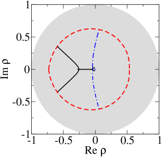
Figure 1: (Color online) An Argand diagram of the Floquet multipliers, $\rho_{i}$, for $b_{0}=1.8$ and $c=1$. The dashed red line indicates the position of the multipliers as $\varepsilon\to 0$, with $\tau\in[\pi/\omega^{*},2\pi/\omega^{*}]$ (cf. Eq. (10)). The blue dot-dashed line shows the location of the multipliers at $\Omega=1.3$, where different points on the line correspond to different values of $\varepsilon>0$. The solid line is for $\Omega=1.7$. The forcing amplitude is varied in the range $\varepsilon\in[10^{-2},1]$. The shaded area is the unit disk.

If the forcing amplitude $\varepsilon$ is small, but non-zero, the deterministic dynamics (II.1) no longer approaches a fixed point, but instead it is found to have a limit cycle. In this limit however, the deterministic trajectory is observed to remain close to the fixed point of the unforced case. The matrix $K(t)$ in Eq. (7) then approaches $K^{*}$ as $\varepsilon\to 0$. It then follows that $\rho_{i}\to\exp\{\lambda_{i}T_{\Omega}\}$, so that the Floquet exponents $\mu_{i}\to\lambda_{i}$ as $\varepsilon\to 0$. We find from a numerical integration of the deterministic dynamics that increasing the level of the forcing amplitude tends to make the forced limit cycle more stable; that is, we find that the modulus of $\rho_{1}$ and $\rho_{2}$ decreases when $\varepsilon$ is increased, as shown in Fig. 1.

Let us end this subsection by returning to the interpretation of complex Floquet multipliers. According to Floquet theory, a solution to Eq. (7) may be written as a linear combination of solutions which have the property $\bm{\xi}_{i}(t+T_{\Omega})=\rho_{i}\bm{\xi}_{i}(t)$ for $i=1,2$. When the $\rho_{i}$ are complex conjugate pairs, this means that linear displacements from the periodic solution $\overline{\mathbf{x}}(t)$ return to the limit cycle in elliptical spirals, in a way similar to the stable fixed point of the unforced case. We illustrate this typical behavior of complex Floquet multipliers in Fig. 2.

Figure 2: (Color online) The top panel is a schematic plot of a deterministic approach, shown as a thin gray (red) curve, to a limit cycle with complex Floquet multipliers; the cycle itself appearing as the closed dark curve (blue). The lower panel, showing a stroboscopic section, illustrates the spiraling return to the limit cycle with a frequency distinct from that of the limit cycle itself.

II.2.3 The case $b_{0}>1+c$

The case in which $b_{0}>1+c$ is slightly more complicated than the one in which the unforced deterministic system approaches a fixed point. For $b_{0}>1+c$ the unforced system has a stable limit cycle solution Boland et al. (2008); we will denote its angular frequency by $\omega_{0}$, where $\omega_{0}$ generally depends on $b_{0}$ and on $c$. One of the Floquet multipliers is equal to unity Boland et al. (2008); Tomita et al. (1974), $\rho_{1}=1$, while the other one is found to be in the range $0<\rho_{2}<1$, consistent with a stable limit cycle attractor. We were not able to find any stable periodic solutions when integrating Eqs. (II.1) at small, but non-zero, forcing amplitudes $\varepsilon$ at generic forcing frequencies. At fixed values of $b_{0}$ and $c$, periodic solutions are however found for all $\Omega$ when the forcing amplitude exceeds a critical value, which we denote by $\varepsilon_{c}(\Omega)$, suppressing a potential dependence on $b_{0}$ and $c$. For $\varepsilon\geq\varepsilon_{c}(\Omega)$ these solutions are stable limit cycles, and the corresponding Floquet multipliers lie within the unit circle. Here we will exclusively focus on this regime. At $\varepsilon=\varepsilon_{c}(\Omega)$ the multipliers have a modulus of one, so that the cycle loses its stability, and as in the previous subsection, increasing the forcing amplitude reduces the moduli of $\rho_{1}$ and $\rho_{2}$, as shown in Fig. 3.

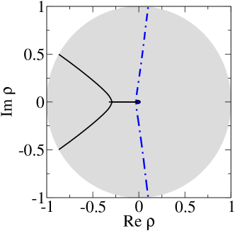
Figure 3: (Color online) Location of the Floquet multipliers in the complex plane for $b_{0}=2.1$ and $c=1$. The dot-dashed blue line is for a forcing frequency of $\Omega=1.3$, the solid black line for $\Omega=1.7$. Periodic solutions are found above $\varepsilon_{c}=0.068$ and $\varepsilon_{c}=0.14$ respectively. Floquet multipliers are shown for $\varepsilon_{c}\leq\varepsilon\leq 1$ for both values of $\Omega$. The shaded area is the unit disk, Floquet multipliers approach the unit circle as $\varepsilon$ approaches $\varepsilon_{c}$ from above.

For our purposes it is sufficient to go on to study the case where the Floquet multipliers remain inside the unit circle, and to analyze the power spectra of stochastic fluctuations about the limit cycle in this regime.

II.3 Stochastic dynamics and system-size expansion

II.3.1 Specification of the Model

We now turn to a discussion of the stochastic microscopic Brusselator system, as defined by the reactions (1)-(4). Labeling the reactions by $\nu=1,\ldots,4$, we denote the rates with which each of the reactions occur by $T_{\nu}(\mathbf{n},t)$. These rates depend on the state of the system $\mathbf{n}=(n_{1},n_{2})$, where $n_{i}$ is the number of molecules of species $X_{i}$, and for the forced system have an additional explicit dependence on time. For the Brusselator system $T_{1}=N$, $T_{2}(\mathbf{n})=n_{1}$, $T_{3}(\mathbf{n},t)=b_{0}(1+\epsilon\cos(\Omega t))n_{1}$ and $T_{4}(\mathbf{n})=cN^{-2}n^{2}_{1}n_{2}$. The combinatorial factors are as in the unforced case Boland et al. (2008). The time-dependent expression for $T_{3}$ reflects the periodic forcing, implemented through an externally-controlled variation of the number of $B$-molecules in the system. We also define the vectors $\mathbf{v}_{\nu}$, $\nu=1,\dots,4$, each capturing the effects of a single occurrence of a reaction of type $\nu$ on the numbers of $X_{1}$ and $X_{2}$ molecules in the system. For the Brusselator $\mathbf{v}_{1}=(1,0)$, $\mathbf{v}_{2}=(-1,0)$, $\mathbf{v}_{3}=(-1,1)$ and $\mathbf{v}_{4}=(1,-1)$ Boland et al. (2008).

II.3.2 Analytical description and system-size expansion

The time evolution of the probability, $P_{\mathbf{n}}(t)$, of finding the system in state $\mathbf{n}$ at time $t$ is then governed by the master equation

$$\frac{\mathrm{d}P_{\mathbf{n}}(t)}{\mathrm{d}t}=\sum_{\nu=1}^{4}\left[T_{\nu}(\mathbf{n}-\mathbf{v}_{\nu},t)P_{\mathbf{n}-\mathbf{v}_{\nu}}(t)-T_{\nu}(\mathbf{n},t)P_{\mathbf{n}}(t)\right].$$ (11)

Solving the master equation analytically is generally not feasible, but an effective description in terms of a Langevin equation, valid at large, but finite, system size can be obtained by means of a van Kampen expansion in the inverse system size van Kampen (2007).

This procedure is well-established and has been applied to a number of microscopic interacting particle systems, so that we do not describe the mathematical details here, but instead refer to van Kampen (2007); McKane et al. (2007). The main idea is to expand realizations $\mathbf{n}(t)$ of the microscopic dynamics about a deterministic trajectory, $\overline{\mathbf{x}}(t)$,

$$\frac{\mathbf{n}(t)}{N}=\overline{\mathbf{x}}(t)+\frac{1}{\sqrt{N}}\bm{\xi}(t),$$ (12)

and to derive an equation of motion for the fluctuations, $\bm{\xi}(t)$, from an expansion of the master equation (11) in powers of $N^{-1/2}$. To lowest order one finds that self-consistency requires $\dot{\overline{\mathbf{x}}}=\mathbf{A}(\overline{\mathbf{x}},t)$, where $\mathbf{A}(\mathbf{x},t)=(A_{1}(\mathbf{x},t),A_{2}(\mathbf{x},t))$ is given by the expressions in Eq. (II.1), recovering the deterministic dynamics of Eqs. (II.1). These equations may also be derived by defining

$$\left\langle{\mathbf{n}(t)}\right\rangle=\sum_{\mathbf{n}}\mathbf{n}P_{\mathbf{n}}(t),$$ (13)

and noting that

$$\frac{\mathrm{d}\left\langle{\mathbf{n}(t)}\right\rangle}{\mathrm{d}t}=\sum_{\nu=1}^{4}\mathbf{v}_{\nu}T_{\nu}\big{(}\left\langle{\mathbf{n}(t)}\right\rangle,t\big{)},$$ (14)

where we have used a deterministic approximation to write $\left\langle{T_{\nu}(\mathbf{n},t)}\right\rangle=T_{\nu}(\left\langle{\mathbf{n}(t)}\right\rangle,t)$. Equations (II.1) are then recovered by setting $\mathbf{x}(t)=\left\langle{\mathbf{n}(t)}\right\rangle/N$. At next-to-leading order the van Kampen expansion gives a linear Langevin equation for the fluctuations, $\bm{\xi}(t)$, about the deterministic trajectory which has the general form van Kampen (2007); McKane et al. (2007)

$$\frac{\mathrm{d}\bm{\xi}(t)}{\mathrm{d}t}=K(t)\bm{\xi}(t)+\mathbf{f}(t),$$ (15)

where, for the forced Brusselator, the matrix $K(t)$ is defined in Eq. (44). The term $\mathbf{f}(t)$ on the right-hand side represents a Gaussian noise of zero mean and with correlator

$$\left\langle{f_{i}(t)f_{j}(t^{\prime})}\right\rangle=2D_{ij}(t)\delta(t-t^{\prime}).$$ (16)

The matrix $D(t)$ may be straightforwardly calculated from the van Kampen expansion van Kampen (2007); McKane et al. (2007). The explicit form for the forced Brusselator is given by Eqs. (45) and (46) in Appendix A.

Equation (15) is a linear Langevin equation, and analytical progress is therefore possible. Of particular interest to us here are the correlation functions and power spectra of the fluctuations $\bm{\xi}(t)$. The time-averaged elements of the covariance matrix $C_{ij}(t,t^{\prime})=\left\langle{\xi_{i}(t)\xi_{j}(t^{\prime})}\right\rangle$ are defined as

$$C_{ij}(\tau)=\frac{1}{T_{\Omega}}\int^{T_{\Omega}}_{0}dt\,\left\langle\xi_{i}(t)\xi_{j}(t+\tau)\right\rangle.$$ (17)

We will in the following mostly focus on the diagonal elements $C_{ii}(\tau)$. Even though Eq. (15) is linear, the analytical computation of $C_{ii}(\tau)$ requires several intermediate steps, and final expressions need to be evaluated numerically. The details are left until the general theory, applicable to systems in an arbitrary number of dimensions, is explained in Sec. IV.

II.3.3 Comparison with simulations

In Fig. 4 we compare results from the analytical calculation just described, with measurements obtained from simulations of the microscopic dynamics. Simulations are carried out using the Gillespie algorithm Gillespie (1977), suitably modified to account for the explicit time-dependence of the reaction rates induced by the external forcing Anderson (2007). Measurements in simulations are taken after a suitable equilibration period in order to minimize the effects of transients. Fig. 4 shows results from the theory (lines) and from simulations (markers), and as seen in the figure, the agreement between them is excellent, both for the time-averaged autocorrelation functions $C_{ii}(\tau)$ and the corresponding power spectra. The latter are obtained as the Fourier transforms of the correlation functions:

$$P_{i}(\omega)=\int~{}d\tau e^{i\omega\tau}C_{ii}(\tau).$$ (18)

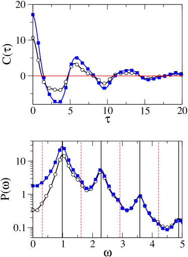
Figure 4: (Color online) The autocorrelation (top panel) and the power spectra (bottom panel) of stochastic fluctuations about the deterministic trajectory of the forced Brusselator. Simulation results for fluctuations $\xi_{1}$ of the number of $X_{1}$-molecules are shown as open circles, while those for $\xi_{2}$ are indicated by full squares. The solid lines are the predictions of the theory, and are seen to match the simulations perfectly. Model parameters are $b_{0}=2.1,c=1,\Omega=1.3$ and $\varepsilon=0.14$. The corresponding non-trivial Floquet multipliers are $\rho=0.023\pm 0.46i$, so that $|\rho|=0.46$. The imaginary part of the Floquet exponent is $\mbox{Im}~{}\mu=0.32$. The system size in simulations is $N=2\times 10^{5}$ and averages over $5000$ independent runs are taken. Vertical lines in the lower panel mark the frequencies of $n\Omega-{\rm Im}\mu$ (solid lines) and $n\Omega+{\rm Im}\mu$ (dashed), where $n$ is a positive integer.

In the numerical simulations we first measure $C_{ii}(t,t^{\prime})$, and then perform a time-average to obtain $C_{ii}(\tau)$. Subsequently a discrete Fourier transform is taken, to obtain $P_{i}(\omega)$. From a practical point of view, $C_{ii}(\tau)$ is found only for $\tau\geq 0$, and then the even nature of the function (discussed later) invoked. Wiesenfeld Wiesenfeld (1985a) suggested peaks would be expected to be seen at frequencies $n\Omega\pm{\rm Im}\mu$, where $n$ is a positive integer and ${\rm Im}\mu$ is $|{\rm Im}\mu_{1,2}|$, where $\mu_{1,2}$ are the two Floquet exponents. However, our results indicate that the presence or otherwise of such peaks depends strongly on the choice of model parameters, and in particular on the position of the Floquet multipliers in the complex plane. For the case shown in Fig. 4, for example, $\rho_{1,2}=0.023\pm 0.46i$ and marked peaks are found at $n\Omega-{\rm Im}\mu$, but not at $n\Omega+{\rm Im}\mu$. A second example is shown in Fig. 5, where we show data for a number of model parameters, resulting in Floquet multipliers much closer to the unit circle than for the example shown in Fig. 4. Peaks are now found at all $n\Omega\pm{\rm Im}\mu$, with the peaks becoming more pronounced as the Floquet multipliers approach the unit circle (from within). In the limit $|\rho_{1,2}|\to 1$, the relaxation of autocorrelation functions becomes very slow and so larger values of $\tau$ need to be taken into account when performing the Fourier transform. This makes both the analytical expressions and the Gillespie simulations more computationally expensive and, for the parameters illustrated in Fig. 5, Gillespie simulation is not feasible.

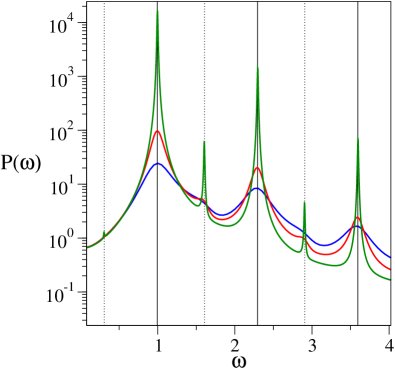
Figure 5: (Color online) Power spectrum of stochastic fluctuations, $\xi_{1}$, in the forced Brusselator system as obtained from the analytical calculations. Model parameters are $b_{0}=2.1$, $c=1$, $\Omega=1.3$, resulting in $\varepsilon_{c}=0.068$. The different curves correspond to forcing amplitude $\varepsilon=0.07,0.11,0.15$, from top to bottom, at the peaks. The corresponding Floquet multipliers have modulus $0.97,0.66$ and $0.41$ respectively. Vertical lines are given at frequencies of $n\Omega-{\rm Im}\mu$ (solid lines) and $n\Omega+{\rm Im}\mu$ (dotted), where $n$ is a positive integer and where $\mbox{Im}\mu\approx 0.31$ for all three cases.

III Willamowski-Rössler system

III.1 Microscopic model

We have seen that forcing the two-dimensional Brusselator opens up the possibility of complex Floquet multipliers. This was not possible in the unforced case since there the deterministic dynamics is autonomous, leading directly to a Floquet multiplier of unity. Therefore, in order to see the effects of complex Floquet multipliers in an autonomous system, the simplest case has three dimensions. One such system is the Willamowski-Rössler model and we shall study the particular form given in Geysermans and Baras (1996, 1997). The model may be written as a chemical reaction system, involving three species $X_{1}$, $X_{2}$ and $X_{3}$, defined by

$$X_{1} \displaystyle\mathrel{\mathop{\vbox{ \hbox{ \ooalign{\raise 1.0pt\hbox{$\relbar\joinrel\rightharpoonup\joinrel$}\crcr\lower 1.0pt\hbox{$\leftharpoondown\joinrel\relbar\joinrel$}} } }}^{b_{1}\mathstrut}_{d_{1}}} 2X_{1},$$ (21)

$$X_{2} \displaystyle\mathrel{\mathop{\vbox{ \hbox{ \ooalign{\raise 1.0pt\hbox{$\relbar\joinrel\rightharpoonup\joinrel$}\crcr\lower 1.0pt\hbox{$\leftharpoondown\joinrel\relbar\joinrel$}} } }}^{b_{2}\mathstrut}_{d_{2}}} 2X_{2},$$ (24)

$$X_{1}+X_{2} \xrightarrow{1} \emptyset,$$ (25)

$$X_{1}+X_{3} \xrightarrow{1}{} 2X_{3},$$ (26)

$$X_{3} \xrightarrow{d_{3}} \emptyset.$$ (27)

The parameters above and below the arrows indicate the relative rates with which each of the reactions occur. Absorbing potential combinatorial factors in the definition of the model parameters $b_{1},b_{2},d_{1}$, and $d_{2}$, the four reactions given in Eqs. (21) and (24) occur with rates $T_{1}(\mathbf{n})=b_{1}n_{1}$, $T_{2}(\mathbf{n})=d_{1}n_{1}^{2}N^{-1}$, $T_{3}(\mathbf{n})=b_{2}n_{2}$ and $T_{4}(\mathbf{n})=d_{2}n_{2}^{2}N^{-1}$. In isolation, these four reactions, (21) and (24), ensure that the average numbers of species $X_{1}$ and $X_{2}$, are of the order of $N$, so that $N$ is again a measure of the system size. We will take the annihilation process (25) to occur with rate $T_{5}(\mathbf{n})=n_{1}n_{2}N^{-1}$; the prefactor in the rate of the reaction is taken to equal unity in order to agree with Geysermans and Baras (1996, 1997). The mathematically interesting limit is that in which the number of $X_{3}$ particles, $n_{3}$, is of order $N$ as well. This is the case when the remaining reaction rates are scaled suitably with $N$. Specifically we will assume that (26) occurs at rate $T_{6}(\mathbf{n})=n_{1}n_{3}N^{-1}$ and (27) at rate $T_{7}(\mathbf{n})=d_{3}n_{3}$. The vectors, $\mathbf{v}_{\nu}$, that correspond to the reactions $\nu=1,\ldots,7$ are given by

$$\mathbf{v}_{1}=(1,0,0), \mathbf{v}_{2}=(-1,0,0),$$

$$\mathbf{v}_{3}=(0,1,0), \mathbf{v}_{4}=(0,-1,0),$$

$$\mathbf{v}_{5}=(-1,-1,0,) \mathbf{v}_{6}=(-1,0,1),$$

$$\mathbf{v}_{7}=(0,0,-1).$$ (28)

III.2 Deterministic Dynamics and Frenet Frame

As in the case of the forced Brusselator, we may now find the equations of the corresponding deterministic dynamics using Eq. (14). For the Willamowski-Rössler model these are

$$\dot{x}_{1}=A_{1}(\mathbf{x}) = x_{1}(b_{1}-d_{1}x_{1}-x_{2}-x_{3}),$$ (29)

$$\dot{x}_{2}=A_{3}(\mathbf{x}) = x_{2}(b_{2}-d_{2}x_{2}-x_{1}),$$ (30)

$$\dot{x}_{3}=A_{3}(\mathbf{x}) = x_{3}(x_{1}-d_{3}).$$ (31)

There are a total of six fixed points of this system, but only one at which all concentrations are non-zero. This fixed point is given by

$$\mathbf{x}^{*}=\left(d_{3},\frac{b_{2}-d_{3}}{d_{2}},b_{1}-d_{1}d_{3}-\frac{b_{2}-d_{3}}{d_{2}}\right).$$ (32)

The stability matrix, $K_{ij}(\mathbf{x})=\partial_{j}A_{i}(\mathbf{x})$, at this fixed point may be found from Eqs. (47) and (48) in Appendix A, by setting $\overline{\mathbf{x}}(t)=\mathbf{x}^{*}$. If the above non-trivial fixed point is unstable then limit cycle solutions of the deterministic equations may exist. Such solutions have, for example, been reported in Geysermans and Baras (1996, 1997), and we will focus on this limit-cycle regime in this section.

Following the notation of the previous sections we will denote the deterministic limit cycle trajectory by $\overline{\mathbf{x}}(t)$, and we will write $\bm{\xi}(t)$ for the fluctuations about it, again as before. Much of the formalism we require has either been discussed in Sec. II, or in Boland et al. (2008). In particular one has an equation of the form (7) within a linear stability analysis of the limit cycle, and in the absense of noise. A direct consequence of the system being autonomous is that the velocity vector, $\dot{\overline{\mathbf{x}}}(t)$, is itself a solution to Eq. (7). Since the velocity is periodic, one of the Floquet multipliers is equal to unity, as it is generally the case for limit cycles of autonomous systems. The dynamics is marginally stable in the direction of the velocity, so that longitudinal fluctuations behave diffusively and may grow without bound in the long run Boland et al. (2008); Tomita et al. (1974). We will focus our interest instead on the fluctuations in the transverse directions, since it is these that have the oscillatory behavior of interest to us. For stable limit cycles and in the absence of persistent noise, these transverse fluctuations decay in a manner characterized by the remaining Floquet multipliers. If the latter are complex, and if the system is subject to intrinsic noise, as induced by the underlying microscopic dynamics at finite system sizes, we expect these fluctuations to be enhanced into quasi-cycles about the limit cycle.

In order to separate longitudinal from transverse modes we need to introduce a suitable frame of reference. Such co-ordinates are provided by the Frenet frame Gibson (2001), which may be constructed by applying the Gram-Schmidt orthogonalization procedure to the first three time derivatives of the limit cycle solution $\overline{\mathbf{x}}(t)$. Specifically, the co-moving basis vectors $\hat{}\mathbf{e}_{i}(t),\,i=1,2,3$ of the Frenet frame are constructed sequentially, as discussed further in Appendix B. The fluctuations are governed by a Langevin equation of the form (15). In order to isolate the transverse fluctuations, we rotate the Langevin equation into the Frenet frame. After the rotation, defined by a matrix, $J(t)$, the Langevin equation takes the form

$$\dot{\mathbf{q}}(t)=K^{\mathrm{tot}}(t)\mathbf{q}(t)+\mathbf{g}(t),$$ (33)

where we follow our earlier paper Boland et al. (2008) and write $\mathbf{q}(t)=J(t)\bm{\xi}(t)$ for the fluctuations in the Frenet frame. The matrix is periodic and given by $K^{\mathrm{tot}}(t)=J(t)K(t)J^{-1}(t)+\dot{J}(t)J^{-1}(t)$ (see Appendix B) and $\mathbf{g}(t)=J(t)\mathbf{f}(t)$ is the rotated noise term. It follows from Eq. (16) that the components of $\mathbf{g}(t)$ are each Gaussian white noise variables with zero mean and correlators

$$\left\langle{g_{i}(t)g_{j}(t^{\prime})}\right\rangle=2G_{ij}(t)\delta(t-t^{\prime}),$$ (34)

where $G(t)=J(t)D(t)J^{-1}(t)$.

For autonomous systems, it is shown in Appendix B that the existence of a longitudinal direction as described above, implies that the elements of the first column of the matrix $K^{\mathrm{tot}}(t)$ vanish, except for the entry in the first row. A consequence of this is that the transverse dynamics may be effectively considered independently of the dynamics in the longitudinal direction. For the Willamowski-Rössler limit cycle this yields a pair of coupled linear Langevin equations in the two transverse directions, with exactly the same mathematical form as those of the forced Brusselator model. Hence the same techniques as before may be applied to produce analytical curves for the autocorrelations and power spectra in the two transverse directions. Note that in our previous work Boland et al. (2008), we were able to simplify the rotated Langevin equations further by a rescaling of the coordinates in the Frenet frame. We do not apply this additional transformation here, since for our purposes it is not essential.

III.3 Stochastic Simulation and Results

The Gillespie algorithm can again be used to generate realizations of the microscopic dynamics defined by Eqs. (21)-(27). Since one Floquet multiplier in the Willamowski-Rössler system is equal to unity, there is a diffusive mode in the longitudinal direction. This means that the time-evolution $(n_{1}(t)/N,n_{2}(t)/N,n_{3}(t)/N)$ of any single realization of this stochastic process may not remain close to the deterministic trajectory $\overline{\mathbf{x}}(t)$, but instead $\left\langle{|\mathbf{n}(t)/N-\overline{\mathbf{x}}(t)|^{2}}\right\rangle\sim t$, where $|\cdot|$ stands for the Euclidean norm. This complication is not present in the driven Brusselator discussed in Sec. II, since in that case no such longitudinal diffusive mode exists.

This issue can however be dealt with as discussed in Boland et al. (2008). The procedure of extracting the deviation from the limit cycle is as follows: for every given data point $\mathbf{n}(t)/N$ generated by the Gillespie algorithm one identifies the point $\overline{\mathbf{x}}(\mathbf{n}(t))$ on the limit cycle trajectory which is geometrically closest to $\mathbf{n}(t)/N$, and then uses $\bm{\kappa}(t)=\mathbf{n}(t)/N-\overline{\mathbf{x}}(\mathbf{n}(t))$ as the displacement vector. As described in Boland et al. (2008) the longitudinal component of $\bm{\kappa}(t)$ vanishes, i.e. one has $\dot{\overline{\mathbf{x}}}.\bm{\kappa}=0$, while the remaining components define a stochastic process in the co-moving transverse plane, and as seen in Boland et al. (2008) the magnitude of $\bm{\kappa}$ remains of order $N^{-1/2}$. This procedure allows one to effectively decouple the diffusive longitudinal mode from the transverse ones, and we will focus on the transverse components in the following, in order to characterize stochastic oscillations about the deterministic limit cycle. These components are then expressed in the Frenet co-ordinates, defined at $\overline{\mathbf{x}}(\mathbf{n}(t))$. As an illustration, trajectories of the transverse components obtained from a single realization of the microscopic dynamics are shown in Fig. 6 for a fixed set of model parameters. In this figure, $N(t)$ denotes the normal component, $N(t)=\bm{\kappa}(t).\hat{\mathbf{e}}_{2}(t)$, and $B(t)$ denotes the deviation from the limit cycle in the binormal direction, $B(t)=\bm{\kappa}(t).\hat{\mathbf{e}}_{3}(t)$. Recall here that $\hat{\mathbf{e}}_{2}$ and $\hat{\mathbf{e}}_{3}$ define a co-moving frame, i.e. that they carry a time-dependence as well.

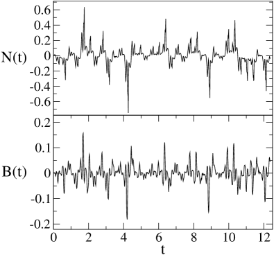
Figure 6: The fluctuations in the directions transverse to the limit cycle trajectory in the Willamowski-Rössler model. Data for the normal component, $N(t)$, and the binormal direction, $B(t)$, are shown for a single realization of the stochastic simulation. Model parameters are $b_{1}=80$, $b_{2}=20$, $d_{1}=0.16$, $d_{2}=0.13$, and $d_{3}=16$.

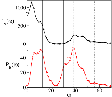
Figure 7: (Color online) Comparison of the theoretical and simulated estimates for the power spectra of transverse fluctuations in the Willamowski-Rössler system. The top panel shows the normal fluctuations (in the direction $\hat{\mathbf{e}}_{2})$ while the bottom panel compares those in the binormal direction, $\hat{\mathbf{e}}_{3}$. Model parameters are again set to $b_{1}=80$, $b_{2}=20$, $d_{1}=0.16$, $d_{2}=0.13$, and $d_{3}=16$. Vertical lines are given at frequencies $n\omega_{0}+\mathrm{Im}\,\mu$ (dotted) and $n\omega_{0}-\mathrm{Im}\,\mu$ (solid), with $n$ a positive integer. The numerical value of $\omega_{0}$ is $17.25$, and the non-trivial Floquet multipliers are $\rho=-0.002\pm 0.303$ (resulting in $|\rho|=0.30$ and $\mbox{Im}~{}\mu=4.33$).

In Fig. 7, we show the resulting power spectra, and find very good agreement between simulation and theory for both the normal and binormal directions. There is a slight systematic deviation of data points from the theory, which occurs at integer multiples of the limit cycle frequency. We attribute these to remnants of the deterministic dynamics. The data shown in Fig. 7 was taken at model parameters resulting in complex Floquet multipliers with a modulus of approximately $0.3$, and peaks are found in the power spectra close to frequencies $n\omega_{0}\pm\mathrm{Im}\,\mu$, where $\omega_{0}$ is the angular frequency of the limit cycle. However, we also note that peaks are not observed at all frequencies $n\omega_{0}\pm\mbox{Im}\mu$, especially in the spectrum of normal fluctuations. As for our findings in the driven Brusselator, this may be due to the fact that the Floquet multipliers in the example shown in Fig. 7 are relatively distant from the unit circle in the complex plane. Again based on our observations in the driven Brusselator one may expect additional peaks at frequencies $n\omega_{0}\pm\mbox{Im}\mu$ to emerge as the Floquet multipliers move closer to the unit circle. Despite an extensive search we have however not been able to find a set of model parameters which would result in Floquet multipliers with modulus close to unity, so that we are not able to give any further confirmation of this expectation here. We conclude this section by re-iterating our main result, the near perfect agreement of the analytically obtained power spectra with simulations as shown in Fig. 7.

IV Generalization to higher dimensions and the coupled Brusselator

IV.1 General theory

It is expected that in the study of any real system, for example in biochemistry or in ecology, the number of distinct species, $S$, would be significantly larger than two or three. It is also possible that solutions to the $S$-dimensional deterministic equations in such a model may be periodic orbits, $\overline{\mathbf{x}}(t)$. Hence, in this section we demonstrate the natural extension of the analysis in the previous sections to models of arbitrary dimension. Whether or not the system is autonomous, we begin with the van Kampen system-size expansion which yields a set of $S$ coupled and linear Langevin equations for stochastic fluctuations, $\bm{\xi}(t)$. We simply note that their form naturally extends to arbitrary dimension and is unchanged from (15), where the $S\times S$ matrix $K(t)$ for the drift is given by $K_{ij}(t)=K_{ij}(\overline{\mathbf{x}}(t))=\partial A_{i}(\overline{\mathbf{x}}(t))/\partial\overline{x}_{j}$, and the symmetric $S\times S$ matrix for diffusion, $D(t)=D(\overline{\mathbf{x}}(t))$, is calculated from the system-size expansion.

The subsequent steps of the analysis then depend on whether the system under consideration is autonomous or not. For non-autonomous systems no rotation is required, and one proceeds directly with the Langevin equation in Cartesian co-ordinates in $S$ dimensions. If the system is autonomous, as in the case of the Willamowski-Rössler model, one first needs to rotate into the $S$-dimensional Frenet frame, and then to separate off the longitudinal component, resulting in a Langevin equation in $S-1$ dimensions for the transverse components. The Frenet frame is defined in $S$ dimensions in Appendix B. This then specifies the rotation matrix $J^{\mathrm{T}}=(\hat{\mathbf{e}}_{1},\ldots,\hat{\mathbf{e}}_{S})$, which is evaluated on the limit cycle so that $J(t)=J(\overline{\mathbf{x}}(t))$. The formalism is a straightforward generalization of that described in Sec. III for the Willamowski-Rössler model, except that there are now $(S-1)$ transverse directions, rather than just two.

Thus, for both autonomous and non-autonomous systems one eventually ends up with a Langevin equation in $d$ dimensions, where $d=S-1$ for the autonomous case, and $d=S$ for non-autonomous systems, such as the driven Brusselator. The further steps of the calculation can hence be discussed simultaneously for the autonomous and non-autonomous cases. As described in more detail in Appendix C, the solution of this Langevin equation can be expressed in terms of any fundamental matrix $X(t)$ of the corresponding homogeneous equation. Since the drift matrix, $K(t)$ (denoted by $\widetilde{K}(t)$ in the autonomous case) is periodic, Floquet theory Grimshaw (1990) asserts that a canonical fundamental matrix may be written in the form $X(t)=P(t)Y(t)$, where $P(t)$ and $Y(t)$ are $d\times d$ matrices. The matrix $P(t)$ is periodic with the same period as the drift matrix while the matrix $Y(t)$ is given by $Y(t)=e^{\mathrm{diag}\{\mu_{1},\ldots,\mu_{d}\}t}$, where the $\mu_{i}$, $i=1,\ldots,d$ are the Floquet exponents of the $d\times d$ homogeneous system.

The periodic matrix, $P(t)$, acting on the left is, in effect, a transformation matrix from the Floquet solutions to the coordinates of the Langevin equation, while its inverse makes the reverse transformation. The matrix $Y(t)$ is a diagonal exponential matrix with entries $e^{\mu_{i}t}$, with ${\rm Re}\mu_{i}<0$, for all $i$, for a stable limit cycle. It therefore acts on different Floquet solutions in different ways, reducing the value of some more quickly than others. The general solution of the Langevin equation (66) which we wish to analyze, can be given in terms of the matrices $P(t)$ and $Y(t)$ and is given explicitly by Eq. (70) in Appendix C.

Given the symmetric and periodic noise matrix, $D(t)$ in the non-autonomous case—which we generally denote by $\widetilde{G}(t)$ using the notation of the autonomous case—we may calculate the autocorrelation function in closed form. In the basis corresponding to the Floquet solutions $\widetilde{G}(t)$ becomes the symmetric and periodic matrix $\Gamma(t)=P^{-1}(t)\widetilde{G}(t)\big{(}P^{-1}\big{)}^{\mathrm{T}}$. These noise contributions are then integrated over one time period of the deterministic limit cycle, $T$, but weighted by decaying exponentials from the $Y(t)$ matrix, to yield another symmetric and periodic matrix, $\Lambda(t)$ (see Eq. (72)), which gives the various covariances of the fluctuations in the space of the Floquet solutions. However, the focus of our interest is in the two-time correlations of the fluctuations which are shown in Appendix C to equal $C(t+\tau,t)=2P(t+\tau)Y(\tau)\Lambda(t)P^{\mathrm{T}}(t)$. Therefore the autocorrelation function itself equals

$$C(\tau)=\frac{2}{T}\int_{0}^{T}P(t+\tau)Y(\tau)\Lambda(t)P^{\mathrm{T}}(t)\mathrm{d}t.$$ (35)

for $\tau\geq 0$. The diagonal elements of $C(\tau)$ turn out to be even functions of $\tau$, as they ought to be. Power spectra, $P_{i}(\omega)$ for $i=1,\ldots,d$, may then be calculated as the Fourier transform of diagonal elements of $C(\tau)$, as in Eq. (18).

IV.2 The case of two coupled Brusselator systems

In order to demonstrate the method on a concrete example, we will study a model composed of two coupled Brusselator systems. Two Brusselator units can be coupled in a number of different ways and here we construct the coupling in such as way as to draw parallels with the forced Brusselator discussed earlier. Chemical species $X_{1}$ and $X_{2}$ form a primary Brusselator through reactions, (1)-(4), with constant populations of $A$, $B$ and $C$. We now also introduce species $X_{3}$, $X_{4}$ and $C^{\prime}$, which follow the reactions,

$$A \rightarrow X_{3}+A,$$ (36)

$$X_{3} \rightarrow \emptyset,$$ (37)

$$X_{3}+X_{2} \rightarrow X_{4}+X_{2},$$ (38)

$$2X_{3}+X_{4}+C^{\prime} \rightarrow 3X_{3}+C^{\prime}.$$ (39)

Given that substance $A$ is part of both units, the secondary Brusselator therefore has the same system size as the primary one. The deterministic dynamics is given by

$$\dot{x}_{1} = 1-x_{1}(1+b-cx_{1}x_{2}),$$ (40)

$$\dot{x}_{2} = x_{1}(b-cx_{1}x_{2}),$$ (41)

$$\dot{x}_{3} = 1-x_{3}(1+x_{2}-c^{\prime}x_{3}x_{4}),$$ (42)

$$\dot{x}_{4} = x_{3}(x_{2}-c^{\prime}x_{3}x_{4}).$$ (43)

When $b>1+c$ there is a limit cycle in the primary Brusselator; we will again denote its angular frequency by $\omega_{0}$. These oscillations of the primary Brusselator act as a periodic forcing on the second, and for all parameters studied here, the second Brusselator shows cycles at the above frequency $\omega_{0}$. The two Brusselators together form a four-dimensional autonomous system. Hence, we will study the fluctuations of the large system-size discrete system which act transverse to the limit cycle. In this example then, we discuss the normal, $\hat{\mathbf{e}}_{2}$, binormal $\hat{\mathbf{e}}_{3}$, and trinormal $\hat{\mathbf{e}}_{4}$, directions. Once the periodic drift $K(t)$ and diffusion $D(t)$ matrices, given by Eqs. (51)-(A.3) in Appendix A, are rotated into the Frenet frame, we then calculate power spectra of transverse fluctuations via Eq. (35). The results of this are presented in Fig. 8 for the model parameters $b=3.3$, $c=2$, and $c^{\prime}=1$.

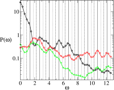
Figure 8: (Color online) Power spectra of the fluctuations about the limit cycles of the coupled Brusselator system. Data is shown for the three transverse directions, with black circles indicating the normal direction, dark gray (red) squares the binormal component, and light gray (green) diamonds the trinormal directions. Markers show results from simulations at a system size of $2\times 10^{5}$ and averaged over $2000$ runs. The solid lines are from the theory, and as seen in the figure the agreement with simulations is near perfect. Vertical lines are shown at frequencies $n\omega_{0}$ (solid), $n\omega_{0}+\mathrm{Im}\,\mu$ (dotted) and $n\omega_{0}-\mathrm{Im}\,\mu$ (dashed), with $n$ a positive integer.

We find very good agreement between theory and simulation performed using the Gillespie algorithm. For these parameters, one of the non-trivial Floquet multipliers, $\rho_{2}$, is real and positive, while the remaining two, $\rho_{\pm}$, take on complex conjugate values. However, these multipliers are not associated with any particular transverse direction, as can be seen from the power spectra: in all three directions, $\hat{\mathbf{e}}_{2}$, $\hat{\mathbf{e}}_{3}$, and $\hat{\mathbf{e}}_{4}$, peaks are found at frequencies equal to a multiple of $\omega_{0}$, but also at those associated with the imaginary parts of the complex Floquet exponents, $\omega_{0}+\mathrm{Im}\,\mu_{\pm}$. While the general formalism we have developed in this section has been illustrated on the concrete example of the coupled Brusselator, it should be clear that it can be applied quite generally to investigate the fluctuations about a limit cycle in $S$-dimensions.

V Conclusions

The phenomenon of stochastic amplification due to demographic, or intrinsic, noise has been qualitatively understood for fifty years, but it is only recently that it has been comprehensively and quantitatively described. This has been due in large part to the application of the technique of the system-size expansion, which is able to reproduce results obtained by numerical simulations to a remarkable precision. In fact, although this method allows for a systematic expansion in powers of $1/\sqrt{N}$, there is usually no need to go beyond next-to-leading order. In essence, application of the method means that the use of numerical simulations to understand the cycles induced by noise could be dispensed with entirely.

If the systems under study are subject to an external periodic driving, for example biological systems subject to an annual cycle, then the deterministic dynamics may have a limit cycle as its stable state. In this paper we have investigated the effect that demographic stochasticity will have on this state. On general grounds one might expect that if the limit cycle was approached in an oscillatory manner, then stochastic cycles about the limit cycle could be sustained. We have shown that once again the system-size expansion may be applied to gain a quantitative understanding of this phenomena. The analysis is considerably more elaborate than in the case where the deterministic dynamics approaches a fixed point, but once again the method gives excellent agreement with numerical simulations.

The signature for the oscillatory approach to limit cycles is that the associated Floquet multiplier should be complex. This can occur for nonautonomous systems in two or more dimensions or autonomous systems in three or more dimensions. Since the eigenvalues of a typical real matrix in these dimensions will generically be complex, one might expect complex Floquet exponents to be common. Our investigations of various models, although far from comprehensive, suggests that they are quite common in periodically driven systems, but not so common in autonomous systems that are generally studied. There may be a dynamical reason for this, but it is as likely that this is due to the nonlinear systems appearing in the literature being selected for their period doubling transition to chaos, rather for the structure of their limit cycles.

In the past it was said that intrinsic noise could turn oscillatory decay to a fixed point into sustained oscillations. It was expected that these oscillations would have periods ${\rm Im}\,\lambda_{i}$, where $\lambda_{i}$ were the eigenvalues of the stability matrix for that fixed point. This is only true in a very broad sense, as studies over the last few years have shown. In reality the period may significantly deviate from ${\rm Im}\,\lambda_{i}$ due to other factors, and the amplitude of the fluctuations may be much larger than might be expected due to a resonance effect. Analogously, one might guess that intrinsic noise could turn oscillatory decay to a limit cycle into sustained oscillations about that cycle and that these oscillations would have periods $n\omega_{0}\pm{\rm Im}\,\mu_{i}$, where $\omega_{0}$ is the period of the limit cycle and $\mu_{i}$ are the Floquet exponents associated with that limit cycle. We have shown in this paper that this is indeed the case in a broad sense, but as for the case of the fixed point there is much more to the story than this. For instance, the expressions $n\omega_{0}\pm{\rm Im}\,\mu_{i}$ are again just an approximation to the frequencies and the amplitude of the oscillations will vary significantly depending on a number of factors, such as the magnitude of the Floquet multipliers. Fortunately, the system-size expansion once again gives results which are in excellent agreement with simulations and gives us a way of exploring the nature of these fluctuations. We expect that the ideas presented in this paper will have a number of applications, which we hope to explore and report on in the future.

Appendix A Explicit Forms of Matrices

The matrices which appear in the description of the fluctuations about the deterministic trajectory are given in this appendix. The drift matrix $K(\mathbf{x})$ and the diffusion matrix $D(\mathbf{x})$ are naturally functions of the concentration $\mathbf{x}$. However, when the solutions of the deterministic dynamics, $\overline{\mathbf{x}}(t+T)=\overline{\mathbf{x}}(t)$, are limit cycles they themselves become periodic functions of time. For the remainder of this appendix, we shall suppress the time dependence of $\overline{\mathbf{x}}(t)$ for greater clarity.

A.1 Forced Brusselator

$$K(t)=\left(\begin{array}[]{rr}-\left[1+b(t)-2c\overline{x}_{1}\overline{x}_{2}\right]&c\overline{x}_{1}^{2}\cr\cr\left[b(t)-2c\overline{x}_{1}\overline{x}_{2}\right]&-c\overline{x}_{1}^{2}\end{array}\right),$$ (44)

$$D(t)=\left(\begin{array}[]{rr}D_{1}(t)&-D_{2}(t)\cr\cr-D_{2}(t)&D_{2}(t)\end{array}\right),$$ (45)

where

$$D_{1}(t) = \frac{1}{2}\left\{1+\overline{x}_{1}\left[1+b(t)+c\overline{x}_{1}\overline{x}_{2}\right]\right\},$$

$$D_{2}(t) = \frac{1}{2}\left\{\overline{x}_{1}\left[b(t)+c\overline{x}_{1}\overline{x}_{2}\right]\right\}.$$ (46)

A.2 Willamowski-Rössler Model

$$K(t)=\left(\begin{array}[]{ccc}K_{11}(t)&-\overline{x}_{1}&-\overline{x}_{1}\cr\cr-\overline{x}_{2}&K_{22}(t)&0\cr\cr\overline{x}_{3}&0&K_{33}(t)\end{array}\right),$$ (47)

where

$$K_{11}(t) = b_{1}-2d_{1}\overline{x}_{1}-\overline{x}_{2}-\overline{x}_{3},$$

$$K_{22}(t) = b_{2}-2d_{2}\overline{x}_{2}-\overline{x}_{1},$$

$$K_{33}(t) = \overline{x}_{1}-d_{3},$$ (48)

and

$$D(t)=\left(\begin{array}[]{ccc}D_{11}(t)&D_{12}(t)&D_{13}(t)\cr\cr D_{12}(t)&D_{22}(t)&0\cr\cr D_{13}(t)&0&D_{33}(t)\end{array}\right),$$ (49)

where

$$D_{11}(t) = \frac{1}{2}\overline{x}_{1}(b_{1}+d_{1}\overline{x}_{1}+\overline{x}_{2}+\overline{x}_{3}),$$

$$D_{12}(t) = \frac{1}{2}\overline{x}_{1}\overline{x}_{2},$$

$$D_{13}(t) = -\frac{1}{2}\overline{x}_{1}\overline{x}_{3},$$

$$D_{22}(t) = \frac{1}{2}\overline{x}_{2}(b_{2}+d_{2}\overline{x}_{2}+\overline{x}_{1}),$$

$$D_{33}(t) = \frac{1}{2}\overline{x}_{3}(\overline{x}_{1}+d_{3}).$$ (50)

A.3 Coupled Brusselators

$$K(t)=\left(\begin{array}[]{rrrr}K_{1}(t)-1&c\overline{x}_{1}^{2}&0&0\cr\cr-K_{1}(t)&-c\overline{x}_{1}^{2}&0&0\cr\cr 0&-\overline{x}_{3}&K_{3}(t)-1&c^{\prime}\overline{x}_{3}^{2}\cr\cr 0&\overline{x}_{3}&-K_{3}(t)&-c^{\prime}\overline{x}_{3}^{2}\end{array}\right),$$ (51)

where

$$K_{1}(t) = 2c\overline{x}_{1}\overline{x}_{2}-b,$$

$$K_{3}(t) = 2c^{\prime}\overline{x}_{3}\overline{x}_{4}-\overline{x}_{2},$$ (52)

and

$$D(t)=\left(\begin{array}[]{rrrr}D_{1}(t)&-D_{2}(t)&0&0\cr\cr-D_{2}(t)&D_{2}(t)&0&0\cr\cr 0&0&D_{3}(t)&-D_{4}(t)\cr\cr 0&0&-D_{4}(t)&D_{4}(t)\end{array}\right),$$ (53)

where in addition to (46) we have,

$$D_{3}(t) = \frac{1}{2}\left[1+\overline{x}_{3}\left(1+\overline{x}_{2}+c^{\prime}\overline{x}_{3}\overline{x}_{4}\right)\right],$$

$$D_{4}(t) = \frac{1}{2}\overline{x}_{3}\left(\overline{x}_{2}+c^{\prime}\overline{x}_{3}\overline{x}_{4}\right).$$ (54)

Appendix B The Frenet Frame

In this appendix we will discuss the background, and develop the formalism, relating to the co-moving frame which we use to study the fluctuations from the limit cycles discussed in the main text. Such a frame, called a Frenet frame Kuhnel (2002), is a natural way to study displacements from a deterministic trajectory in any number of dimensions. Here we will denote the number of dimensions by $S$.

Consider the general autonomous problem which we may describe by a system of non-linear, homogeneous, first-order equations,

$$\frac{\mathrm{d}\mathbf{x}}{\mathrm{d}t}=\mathbf{A}(\mathbf{x}).$$ (55)

Following Kuhnel (2002), we may define the Frenet frame by applying the Gram-Schmidt orthogonalization procedure to the time-derivatives of the solution, $\mathbf{x}(t)$. So long as the time derivatives are linearly independent, this gives the basis vectors, $\hat{\mathbf{e}}_{i}(t)$, of the frame to be

$$\mathbf{e}_{i}(t) = \frac{\mathrm{d}^{i}{\mathbf{x}}(t)}{\mathrm{d}t^{i}}-\sum_{j=1}^{i-1}\left(\frac{\mathrm{d}^{i}{\mathbf{x}}(t)}{\mathrm{d}t^{i}}\cdot\hat{\mathbf{e}}_{j}(t)\right)\hat{\mathbf{e}}_{j}(t),$$ (56)

$$\hat{\mathbf{e}}_{i}(t) = \frac{\mathbf{e}_{i}(t)}{\left|\mathbf{e}_{i}(t)\right|},\ i\in\{1,\ldots,S\}.$$ (57)

We may now construct the matrix which transforms from Cartesian co-ordinates to the Frenet frame to be $J(t)=\left(\hat{\mathbf{e}}_{1}(t),\ldots,\hat{\mathbf{e}}_{S}(t)\right)^{\mathrm{T}}$. The transformation is by construction an orthogonal matrix $\mathrm{O}(S)$, and as such has the property that $J^{\mathrm{T}}(t)=J^{-1}(t)$ for all times.

We now wish to consider the effect of this transformation on the equation of a linear fluctuation, $\bm{\xi}(t)$, about the deterministic solution, $\overline{\mathbf{x}}(t)$. For the time being we will neglect the noise term and consider the homogeneous equation, $\dot{\bm{\xi}}(t)=K(t)\bm{\xi}(t)$. The transformation to the Frenet frame takes the form $\bm{\xi}(t)\mapsto\mathbf{q}(t)=J(t)\bm{\xi}(t)$. Then $\dot{\bm{\xi}}(t)=(\dot{J}(t)+J(t)K(t))\bm{\xi}(t)$ and so the rotated displacement obeys the linear equation,

$$\dot{\mathbf{q}}(t)=K^{\rm tot}(t)\mathbf{q}(t),$$ (58)

where $K^{\rm tot}(t)=K^{\prime}(t)+R(t)$ and where

$$K^{\prime}(t)=J(t)K(t)J^{-1}(t),\ R(t)=\dot{J}(t)J^{-1}(t).$$ (59)

We now evaluate the elements of the first column of the matrix $K^{\rm tot}$. These have an especially simple form, with $K^{\rm tot}_{i1}=0$ for $i>1$. This follows from the fact that, for an autonomous system, $\ddot{\overline{\mathbf{x}}}(t)=K(t)\dot{\overline{\mathbf{x}}}(t)$, and so the “velocity” $\dot{\overline{\mathbf{x}}}(t)$, is a solution of the homogeneous equation that we are considering. From this, and from $\hat{\mathbf{e}}_{1}(t)=\dot{\overline{\mathbf{x}}}(t)/|\dot{\overline{\mathbf{x}}}(t)|$, it follows that

$$K^{\prime}_{i1}(t)=\frac{1}{|\dot{\overline{\mathbf{x}}}(t)|}\hat{\mathbf{e}}_{i}(t)\cdot\ddot{\overline{\mathbf{x}}}(t).$$ (60)

The second term in the definition of $K^{\rm tot}(t),R(t)$, may be written in terms of the basis vectors and, due to their orthogonality properties, we have

$$R_{i1}(t)=\frac{\mathrm{d}\hat{\mathbf{e}}_{i}(t)}{\mathrm{d}t}\cdot\hat{\mathbf{e}}_{1}(t)=-\hat{\mathbf{e}}_{i}(t)\cdot\frac{\mathrm{d}\hat{\mathbf{e}}_{1}(t)}{\mathrm{d}t},$$ (61)

for $i\neq 1$. The rate of change of the longitudinal basis vector is given by $\big{(}\ddot{\overline{\mathbf{x}}}(t)-\hat{\mathbf{e}}_{1}(\hat{\mathbf{e}}_{1}\cdot\ddot{\overline{\mathbf{x}}}(t))\big{)}/|\dot{\overline{\mathbf{x}}}(t)|$ and so

$$R_{i1}(t)=-\frac{1}{|\dot{\overline{\mathbf{x}}}(t)|}\hat{\mathbf{e}}_{k}(t)\cdot\ddot{\overline{\mathbf{x}}}(t),\ i\neq 1.$$ (62)

Adding Eqs. (60) and (62), and noting that $R_{11}=0$, we have

$$K^{\rm tot}_{i1}(t)=0\ (i>1);\ K^{\rm tot}_{11}(t)=\frac{1}{|\dot{\overline{\mathbf{x}}}(t)|^{2}}\dot{\overline{\mathbf{x}}}(t)\cdot\ddot{\overline{\mathbf{x}}}(t).$$ (63)

So all of the elements of the first column of $K^{\rm tot}(t)$ vanish, apart from the element which is also in the first row. The significance of this is that the transverse displacements, which we denote by $\mathbf{r}(t)$ decouple from the longitudinal displacements, denoted by $s(t)$. So writing a general displacement as $\mathbf{q}(t)=(s(t),\mathbf{r}(t))$, we have

$$\dot{s}(t) = K^{\rm tot}_{11}(t)s(t)+\mathbf{K}_{sr}(t)\cdot\mathbf{r}(t),$$ (64)

$$\dot{\mathbf{r}}(t) = \widetilde{K}(t)\mathbf{r}(t),$$ (65)

where the vector $\mathbf{K}_{sr}(t)$ is the $(S-1)$-dimensional vector $K^{\rm tot}_{1i}(t)$ and where $\widetilde{K}(t)$ now describes the purely transverse drift behavior. So the Frenet frame always separates the equation of motion for the linear fluctuations into longitudinal and transverse parts and the transverse motion is free from any influence by the longitudinal motion.

Appendix C Autocorrelations of Periodic Langevin Equations

The equations which describe small perturbations about the limit cycle either have the form (7) for non-autonomous (forced) systems or the form (65) for autonomous (unforced) systems. In the latter case longitudinal displacements have been excluded, but once this has been done, the analysis for both cases is identical. So we can develop the theory for both together, we will adopt the notation of the autonomous case, that is, start from the equation $\dot{\mathbf{r}}(t)=\widetilde{K}(t)\mathbf{r}(t)$. It should then be understood that in the non-autonomous case the replacements $\mathbf{r}(t)\to\bm{\xi}(t)$ and $\widetilde{K}(t)\to K(t)$ should be made.

The results of Floquet theory Grimshaw (1990) tell us that, when $\widetilde{K}(t+T)=\widetilde{K}(t)$ for all $t$, one may generally find $d$ linearly independent solutions to the homogeneous equation $\dot{\mathbf{r}}(t)=\widetilde{K}(t)\mathbf{r}(t)$ which have the form $\mathbf{r}(t)=\mathbf{p}_{i}(t)\mathrm{e}^{\mu_{i}t}$. Here $\mu_{i}$, $i=1,\ldots,d$, are the Floquet exponents, which may in general be complex, and the functions $\mathbf{p}_{i}(t)$ are periodic with the period, $T$. From these solutions, the the canonical fundamental matrix, $X(t)$, may be constructed. It has the special property that the constant Floquet matrix, $B=X^{-1}(t)X(t+T)$, is diagonal with elements equal to the Floquet multipliers. Grimshaw Grimshaw (1990) appends a subscript $0$ to denote the canonical choice which results in a diagonal Floquet matrix, but since we will only deal with such a choice in this paper, we omit this subscript. However when carrying out numerical work, it should be recognized that in general the solutions which are found will be linear combinations of solutions of the form $\mathbf{p}_{i}(t)\mathrm{e}^{\mu_{i}t}$. These can be used to find a (non-diagonal) $B$, the eigenvectors of which can be used to construct a similarity transformation to a canonical form. An alternative way of describing the canonical solutions is to define the periodic matrix $P(t)=(\mathbf{p}_{1}(t),\ldots,\mathbf{p}_{d}(t))$ and the diagonal exponential matrix $Y(t)=\exp\{\mathrm{diag}(\mu_{1}\ldots\mu_{d})t\}$. In terms of these the canonical fundamental matrix is given by $X(t)=P(t)Y(t)$.

Moving on to the fluctuations about the periodic solutions of the deterministic dynamics, the linear stochastic fluctuations obey a Langevin equation (15), with the noise correlator given by Eq. (16), for non-autonomous (forced) systems and a Langevin equation (33), with the noise correlator given by Eq. (34), where $G(t)=J(t)D(t)J^{-1}(t)$, for autonomous (unforced) systems. To separate out the latter into longitudinal and transverse components, we note that in Appendix B we wrote $\mathbf{q}(t)=(s(t),\mathbf{r}(t))$, and now we analogously write $\mathbf{g}(t)=(g_{s}(t),\mathbf{g}_{r}(t))$. Then, since the transverse fluctuations decouple from the longitudinal fluctuations, the Langevin equation for purely transverse fluctuations $\mathbf{r}(t)$ may be written as

$$\dot{\mathbf{r}}(t)=\widetilde{K}(t)\mathbf{r}(t)+\mathbf{g}_{r}(t).$$ (66)

The noise correlator (34) can be expressed in terms of transverse and longitudinal components by decomposing $G(t)$ as follows:

$$G(t)=\left(\begin{array}[]{cc}G_{ss}(t)&\mathbf{G}^{\mathrm{T}}_{sr}(t)\\ \mathbf{G}_{sr}(t)&\widetilde{G}(t)\end{array}\right).$$ (67)

Since the vector $\mathbf{G}_{sr}(t)$ is typically non-zero, the random variables, $g_{s}$ and $\mathbf{g}_{r}$, generally remain statistically correlated in the rotated frame. However, this is only important if we intend to evaluate simultaneous values of both $g_{s}(t)$ and $\mathbf{g}_{r}(t)$ and this we do not do, because we have already shown for the noiseless case that the transverse displacements are independent of longitudinal one. Therefore the only noise correlator we require is

$$\left\langle{\mathbf{g}_{r}(t)\cdot\mathbf{g}_{r}^{\mathrm{T}}(t^{\prime})}\right\rangle=2\widetilde{G}(t)\delta(t-t^{\prime}).$$ (68)

Once again we will develop the theory using the notation of Eqs. (66) and (68), but it applies equally to Eqs. (15) and (16).

Floquet theory may be applied to linear inhomogeneous equations of the form (66), as well as to homogeneous equations such as $\dot{\mathbf{r}}(t)=\widetilde{K}(t)\mathbf{r}(t)$ Grimshaw (1990). To solve Eq. (66), we proceed in the standard way and add a particular solution of the equation to a general solution of the corresponding homogeneous equation. This yields Grimshaw (1990)

$$\mathbf{r}(t)=X(t)\mathbf{r}_{0}+X(t)\int_{t_{0}}^{t}X^{-1}(s)\mathbf{g}_{r}(s)\mathrm{d}s,$$ (69)

for $t\geq t_{0}$ and with the initial condition $\mathbf{r}(t_{0})=X(t_{0})\mathbf{r}_{0}$. Since we will not be interested in the effects of transients in this paper, we set the initial conditions in the infinitely distant past, $t_{0}\to-\infty$. A change of integration variable $s\to s^{\prime}=t-s$ in the solution (69) now gives

$$\mathbf{r}(t)=P(t)\int_{0}^{\infty}Y(s^{\prime})P^{-1}(t-s^{\prime})\mathbf{g}_{r}(t-s^{\prime})\mathrm{d}s^{\prime},$$ (70)

where we have used the fact that, since $Y(t)$ is a diagonal exponential matrix, $Y(t_{1}+t_{2})=Y(t_{1})Y(t_{2})$.

Of course, $\mathbf{r}(t)$ is a stochastic variable, and we will typically be interested in finding correlation functions, principally the two-time correlation function $C(t+\tau,t)=\left\langle{\mathbf{r}(t+\tau)\mathbf{r}^{\mathrm{T}}(t)}\right\rangle$. Taking $\tau\geq 0$, the solution (70) gives

$$C(t+\tau,t)=2P(t+\tau)Y(\tau)\Lambda(t)P^{\mathrm{T}}(t),$$ (71)

where we have introduced the symmetric and periodic matrix integral,

$$\Lambda(t)=\int_{0}^{\infty}Y(s)\Gamma(t-s)Y(s)\mathrm{d}s,$$ (72)

and, in turn, the symmetric and periodic matrix

$$\Gamma(s)=P^{-1}(s)\widetilde{G}(s)\left(P^{-1}(s)\right)^{\mathrm{T}}.$$ (73)

All of the functions in Eq. (71) are deterministic and may be evaluated given a good numerical estimate for the limit cycle solution $\overline{\mathbf{x}}(t)$.

The infinite integral for $\Lambda(t)$ may be evaluated as a re-summed finite integral due to the periodicity of $\Gamma(s)$. The result, in terms of Floquet multipliers, $\rho_{i}$, is then,

$$\Lambda_{ij}(t)=\frac{1}{1-\rho_{i}\rho_{j}}\int_{0}^{T}\mathrm{e}^{(\mu_{i}+\mu_{j})s}\Gamma_{ij}(t-s)\mathrm{d}s,$$ (74)

for $i,j=1,\dots,d$. The origin of the prefactor is from an infinite geometric summation, $\sum_{n=0}^{\infty}(\rho_{i}\rho_{j})^{n}$, which is convergent when the Floquet multipliers are inside the unit circle.

Finally, although the details are not presented here, an expression can be found for $\tau<0$. It turns out that $C(\tau)=C(-\tau)^{\mathrm{T}}$, as it ought. Hence the final form is given by Eq. (35) for $\tau\geq 0$, and can be found from Eq. (35) for $\tau\leq 0$, supplemented by the condition $C(\tau)=C(-\tau)^{\mathrm{T}}$.