A theory of amorphous packings of binary mixtures of hard spheres

Abstract

We extend our theory of amorphous packings of hard spheres to binary mixtures and more generally to multicomponent systems. The theory is based on the assumption that amorphous packings produced by typical experimental or numerical protocols can be identified with the infinite pressure limit of long lived metastable glassy states. We test this assumption against numerical and experimental data and show that the theory correctly reproduces the variation with mixture composition of structural observables, such as the total packing fraction and the partial coordination numbers.

Amorphous packings of hard spheres are ubiquitous in physics: they have been used as models for liquids, glasses, colloidal systems, granular systems, and powders. They are also related to important problems in mathematics and information theory, such as digitalization of signals, error correcting codes, and optimization problems. Moreover, the structure and density (or porosity) of amorphous multicomponent packings is important in many branches of science and technology, ranging from oil extraction to storage of grains in silos.

Despite being empirically studied since at least sixty years, amorphous packings still lack a precise mathematical definition, due to the intrinsic difficulty of quantifying “randomness” Torquato et al. (2000). Indeed, even if a sphere packing is a purely geometrical object, in practice dense amorphous packings always result from rather complicated dynamical protocols: for instance, spheres can be thrown at random in a box that is subsequently shaken to achieve compactification Scott and Kilgour (1969), or they can be deposited onto a random seed cluster Bennett (1972). In numerical simulations, one starts from a random distribution of small spheres and inflates them until a jammed state is reached Lubachevsky and Stillinger (1990); Donev et al. (2006); alternatively, one starts from large overlapping spheres and reduces the diameter in order to eliminate the overlaps Jodrey and Tory (1985); Clarke and Jónsson (1993); O’Hern et al. (2002); Lochmann et al. (2006). In principle, each of these dynamical prescriptions produces an ensemble of final packings that depends on the details of the procedure used. Still, very remarkably, if the presence of crystalline regions is avoided, the structural properties of amorphous packings turn out to be very similar. This observation led to the proposal that “typical” amorphous packings should have common structure and density; the latter has been denoted Random Close Packing (RCP) density. The definition of RCP has been intensively debated in the last few years, in connection with the progresses of numerical simulations Torquato et al. (2000); Kamien and Liu (2007).

Nevertheless, the empirical evidence, that amorphous packings produced according to very different protocols have common structural properties, is striking and call for an explanation. This is all the more true for binary or multicomponent mixtures, where in addition to the usual structural observables, such as the structure factor, one can investigate other quantities such as the coordination between spheres of different type, and study their variation with the composition of the mixture.

In earlier attempts to build statistical models of packings, only the main geometrical factors, such as the relative size and abundance of the different components, were taken into account Dodds (1975, 1980); Ouchiyama and Tanaka (1981). More precisely, these models focus on a random sphere in the packing and its first neighbors, completely neglecting spatial correlations beside the first shell and all the global geometric constraints. This already accounts for the main qualitative structural properties of random packings. However, in order to obtain a quantitative description, some free parameters have to be introduced and adjusted to match with experimental data.

To go beyond these simple models, many authors proposed that random packings of hard spheres can be thought as the infinite pressure limit of hard sphere glasses Woodcock and Angell (1981); Stoessel and Wolynes (1984); Speedy (1998); Cardenas et al. (1998); Parisi and Zamponi (2005); Krzakala and Kurchan (2007); Parisi and Zamponi (2008). This is very intuitive since a glass is a solid state in which particles vibrate around amorphous reference positions, and vibrations are reduced on increasing pressure. A typical algorithm attempting to create a random packing starts at low density and compresses the system at a given rate. During this evolution, when the density is high enough, relaxation becomes more and more difficult until at some point the system is stuck into a glass state Krzakala and Kurchan (2007); Parisi and Zamponi (2008); at this point further compression will only reduce the amplitude of the vibrations. In a nutshell, this is why amorphous packings can be identified with glasses at infinite pressure.

The main advantage of this identification, if it holds, is that a glass is a metastable state that has a very long lifetime; therefore, its properties can be studied using concepts of equilibrium statistical mechanics. In this way a complicated dynamical problem (solving the equations of motion for a given protocol) is reduced to a much more simple equilibrium problem. In Parisi and Zamponi (2005, 2008) it was shown, in the case of monodisperse packings, that this strategy is very effective since it allows to compute structural properties of random packings directly from the Hamiltonian of the system, without free parameters and in a controlled statistical mechanics framework. Note that the existence of an equilibrium glass transition in hard sphere systems (or in other words the existence of glasses with infinite life time) has been questioned Donev et al. (2006); Santen and Krauth (2000). Although very interesting, this problem is not relevant for the present discussion since we are only interested in long-lived metastable glasses that trap dynamical algorithms. At present it is very well established by numerical simulations Berthier and Witten (2008, 2009) that for system sizes of $N\lesssim 10^{4}$ particles and on the time scales of typical algorithms, metastable glassy states exist, at least in $d\geq 3$. This is enough to compare with most of the currently available numerical and experimental data. Finally, the relation of this approach to special packings such as the MRJ state Torquato et al. (2000) and the J-point O’Hern et al. (2002) has been discussed in detail in Parisi and Zamponi (2008).

The aim of this paper is to extend the theory of Parisi and Zamponi (2005, 2008) to binary mixtures. This allows to compare quantitatively the predictions of the theory and the results of numerical simulations. We will focus in particular on the variation of density and local connectivity as a function of mixture composition. These results constitute, in our opinion, a stringent test of the assumption that random packings reached by standard algorithms can be identified with infinite pressure metastable glasses.

Theory - The equilibrium statistical mechanics computation of the properties of the glass is based on standard liquid theory Hansen and McDonald (1986) and on the replica method Cardenas et al. (1998); Mézard and Parisi (1999) that has been developed in the context of spin glass theory Mézard et al. (1987); Monasson (1995). For monodisperse hard spheres, it has been described in great detail in Parisi and Zamponi (2008). The extension to multicomponent systems is straightforward following Coluzzi et al. (1999); details are given in Appendix.

Here we just recall some features of this approach, based on simple physical considerations. The basic assumption of the method are that i) crystallization and phase separation are strongly suppressed by kinetic effects so that the liquid can be safely followed at high density, and ii) that at sufficiently high density, the liquid is a superposition of a collection of amorphous metastable states. Namely, in the liquid, the system spends some time inside one of these states, and sometimes undergoes a rearrangement that leads to a different state Goldstein (1969). Each state is characterized by its vibrational entropy per particle, denoted by $s$, and the number of such states is assumed to be exponential in $N$, so defining a configurational entropy $\Sigma(\varphi,s)=N^{-1}\log{\cal N}(\varphi,s)$, being ${\cal N}(\varphi,s)$ the number of states having entropy $s$ at density $\varphi$. On increasing the density, the liquid is trapped for longer and longer times into a metastable state, until at some point the transition time becomes so long that for all practical purposes the system is stuck into one state: it then becomes a glass. To compute the properties of the glassy states, the central problem is to compute the function $\Sigma(\varphi,s)$. This can be done by means of a simple replica method introduced by Monasson Monasson (1995). One introduces $m$ copies of each particle, constrained to be close enough, in such a way that they must be in the same metastable state. Then, the total entropy of the system of $m$ copies is given by $\SS(m,\varphi|s)=ms+\Sigma(\varphi,s)$; the first term gives the entropy of the $m$ copies in a state of entropy $s$, while the second term is due to the multiplicity of possible states. The total entropy of the system at fixed density $\varphi$ is obtained by maximizing over $s$, i.e.

$$\SS(m,\varphi)=\max_{s}[\Sigma(\varphi,s)+ms]=\Sigma(\varphi,s^{*})+ms^{*}\ ,$$ (1)

where $s^{*}(m,\varphi)$ is determined by the condition $\partial_{s}\Sigma(\varphi,s)=m$. Then it immediate to show that

$$\begin{split}&s^{*}(m,\varphi)=\partial_{m}\SS(m,\varphi)\ ,\\ &\Sigma(\varphi,s^{*}(m,\varphi))=-m^{2}\partial_{m}[\SS(m,\varphi)/m]\ .\end{split}$$ (2)

The knowledge of $\SS(m,\varphi)$ allows to reconstruct the curve $\Sigma(\varphi,s)$ for a given density by a parametric plot of Eqs. (2) by varying $m$. The function $\Sigma(\varphi,s)$ gives access to the internal entropy and the number of metastable glassy states; from this one can compute their equation of state, i.e. the pressure as a function of the density; in particular, for each set of glassy states of given configurational entropy $\Sigma_{j}$, one can compute the density $\varphi_{j}$ (jamming density) at which their pressure diverges. Since $\varphi_{j}$ turns out to depend (slightly) on $\Sigma_{j}$, a prediction of the theory is that different glasses will jam at different density: amorphous packings can be found in a finite (but small) interval of density Krzakala and Kurchan (2007); Parisi and Zamponi (2008).

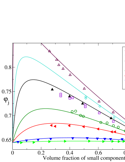
Figure 1: (Color online) Packing fraction $\varphi_{j}$ as a function of $\eta=1/(1+xr^{3})$ at fixed $r$. Full symbols are numerical data from this work. Open symbols are experimental results from Ref. Yerazunis et al. (1965). Lines are predictions from theory, obtained fixing $\Sigma_{j}=1.7$. Note that the large $r$-small $\eta$ region could not be explored, since for such very asymmetric mixtures the large spheres form a rigid structure while small spheres are able to move through the pores and are not jammed Dodds (1980); Ouchiyama and Tanaka (1981).

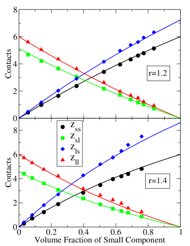
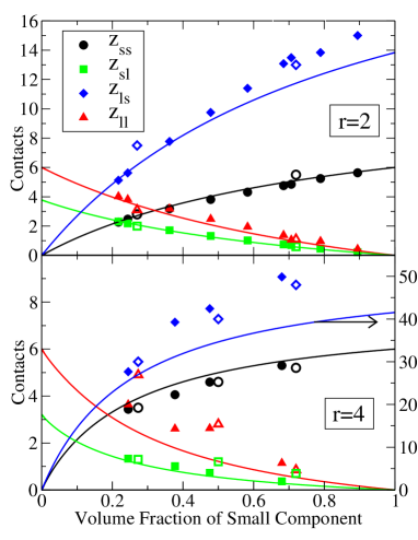
Figure 2: (Color online) Partial average coordination numbers (small-small, small-large, large-small, large-large) as a function of volume fraction of the small particles $\eta=1/(1+xr^{3})$ for different values of $r$. Full symbols are numerical data from this work. Open symbols are experimental data from Ref. Pinson et al. (1998). Note that in the lower right panel a different scale is used for $z_{ls}$.

Results for binary mixtures - The details of the computation of the function $\SS(m,\varphi)$ for a general multicomponent mixture, based on Parisi and Zamponi (2008), can be found in Appendix. Here we consider a binary mixture of two types of spheres $\mu=A,B$ in a volume $V$, with different diameter $D_{\mu}$ and density $\rho_{\mu}=N_{\mu}/V$. We define $r=D_{A}/D_{B}>1$ the diameter ratio and $x=N_{A}/N_{B}$ the concentration ratio; $V_{3}(D)=\pi D^{3}/6$ the volume of a three dimensional sphere of diameter $D$; $\varphi=\rho_{A}V_{3}(D_{A})+\rho_{B}V_{3}(D_{B})$ the packing fraction; $\eta=\rho_{B}V_{3}(D_{B})/\varphi=1/(1+xr^{3})$ the volume fraction of the small ($B$) component.

Once an equation of state for the liquid has been chosen, the jamming packing fraction $\varphi_{j}$ is given in term of $\Sigma_{j}$ by the solution of $\Sigma_{j}(\varphi)=\Sigma_{j}$. The average coordination numbers at $\varphi_{j}$ are denoted $z_{\mu\nu}(\varphi_{j})$, but we checked that their variations with $\varphi_{j}$ are negligible. We used in $d=3$ the equation of state proposed in Santos et al. (2005), using the Carnahan-Starling equation for the monodisperse system Hansen and McDonald (1986). The latter, as well as $\Sigma_{j}(\varphi)$ and $z_{\mu\nu}(\varphi_{j})$, are given respectively in Eqs. (20), (16), (19), in Appendix.

Numerical simulations - We produced jammed packings of binary mixtures of $N=1000$ hard spheres using the code developed by Donev et al. Donev et al. (2005); Donev and Torquato (2005). In this algorithm spheres are compressed uniformly by increasing their diameter at a rate $dD/dt=2\gamma$ while event-driven molecular dynamics is performed at the same time. In order to obtain a perfectly jammed final packing, the later stages of compression must be performed very slowly. On the other hand, at low density slow compression is a waste of time, since the dynamics of the system is very fast. Following Skoge et al. (2006), we find a good compromise by performing a four stages compression: starting from random configurations at $\varphi=0.1$, i) the first stage is a relatively fast compression ($\gamma=10^{-2}$) up to a reduced pressure $p=\beta P/\rho=10^{2}$; then we compress at ii) $\gamma=10^{-3}$ up to $p=10^{3}$; iii) $\gamma=10^{-4}$ up to $p=10^{9}$; iv) $\gamma=10^{-5}$ up to $p=10^{12}$. The first stage terminates at a density $\varphi\sim 0.6$, and is fast enough to avoid crystallization and phase separation. During the following stages the system is already dense enough to stay close to the amorphous structure reached during the first stage. Still, little rearrangements (involving many particles) are possible and allow to reach a collectively jammed final state Skoge et al. (2006). In the final configurations, we observe a huge gap between contacting (typical gap $\sim 10^{-11}D$) and non-contacting (typical gap $\gtrsim 10^{-6}D$) particles. We then say that two particles are in contact whenever the gap is smaller than $10^{-8}D$. Typically, a small fraction ($\lesssim 5\%$ of the total) of rattlers, i.e. particles having less then 4 contacts, is present. Once these are removed, the configuration is isostatic (the total number of contacts is $6N$) within $1\%$ accuracy.

Comparison of theory and numerical/experimental data - During the four stages of compression, the pressure initially follows the liquid equation of state up to some density close to the glass transition density Parisi and Zamponi (2008); Götze and Voigtmann (2003); Foffi et al. (2003). Above this density, pressure increases faster and diverges on approaching jamming at $\varphi_{j}$. The exact point where this happens depends on compression rate. This is a nice confirmation of a prediction of the theory, that different glassy states jam at different density; it was already observed in Donev et al. (2006); Skoge et al. (2006) and recently discussed in great detail in Berthier and Witten (2009); Hermes and Dijkstra (2009). Within the theory $\varphi_{j}$ is related to $\Sigma_{j}$, the value of configurational entropy at which the system falls out of equilibrium; hence there is one free parameter, $\Sigma_{j}$, that depends on the compression protocol. The equation of state of the glass obtained numerically with our protocol corresponds within our theory to $\Sigma_{j}\sim 1.5$. We decided to use the value $\Sigma_{j}=1.7$ that gives the best fit to the numerical data. This is consistent with previous observations, that the configurational entropy is close to $1$ when the system falls out of equilibrium Angelani and Foffi (2007). A detailed discussion of the behavior of pressure can be found in Appendix.

In figure 1, we report the jamming density for different mixtures, putting together our numerical results and experimental data from Ref. Yerazunis et al. (1965), and the theoretical results. Note that a single “fitting” parameter $\Sigma_{j}$, that is strongly constrained, allows to describe different sets of independent numerical and experimental data. The prediction of our theory are qualitatively similar to previous ones Dodds (1980); Ouchiyama and Tanaka (1981), but the quantitative agreement is much better. Interestingly, a similar qualitative behavior for the glass transition density has been predicted in Götze and Voigtmann (2003); Foffi et al. (2003); although there is no a priori reason why the jamming and glass transition density should be related Berthier and Witten (2009), it is reasonable to expect that they show similar trends Foffi et al. (2003).

Finally, in figure 2 we report the average partial contact numbers for different mixtures. These values have been obtained by removing the rattlers from the packing. As discussed above, the total coordination is close to the isostatic value $z=6$. This is also a non trivial prediction of the theory, see Appendix. As it can be seen from figure 2, the computed values agree very well with the outcome of the numerical simulation, at least for $r$ not too large. Some discrepancies are observed in the contacts of the large particles for large $r$. We produced packings of $N=10^{4}$ and checked that these are not finite size effects. Also, inspection of the configurations seem to exclude the presence of phase separation. However, for these values of $r$ and $x$, a large fraction of rattlers ($\sim 10\%$) is present within the small particles. This might affect the determination of the partial contacts. It would be interesting to check if better results are obtained using different algorithms. Experimental data from Pinson et al. (1998) are also reported in the right panel of figure 2.

Conclusions - In this paper we have extended our theory of amorphous packings to binary mixtures and have tested it against numerical and experimental data. In particular we have shown that the theory correctly predicts the variation of total density (or porosity) and local coordination with mixture composition. We have also shown that the behavior of pressure during compression follows the predictions of the theory. A striking prediction of the theory is that different compression procedures lead to different final densities, which seems to be confirmed by numerical data, see also Berthier and Witten (2009); Hermes and Dijkstra (2009). Note that the only free parameter is the value of $\Sigma_{j}$, that is still strongly constrained (it must be close to 1). It affects slightly the values of density (by varying $\Sigma_{j}$ in the reasonable range one can change $\varphi_{j}$ of $\sim 10\%$, see figure 3 in Appendix) and does not affect at all the curves in figure 2 for the local coordinations. As stated in the introduction, we believe that these results constitute a stringent test of the idea that amorphous packings can be considered as the infinite pressure limit of metastable glassy states. Note that our results have no implications on the existence of an ideal glass transition Santen and Krauth (2000); Donev et al. (2006). Indeed, we only used numerical data obtained using fast compressions. It is possible that using much slower compressions physics changes dramatically and the glass transition is avoided. Still, these time scales are out of reach of current algorithms and experimental protocols.

Acknowledgments - We wish to thank A. Donev for his invaluable help in using his code, and L. Berthier for many important suggestions and for providing equilibrated configurations at high density.

Appendix

I Behavior of the pressure during compression

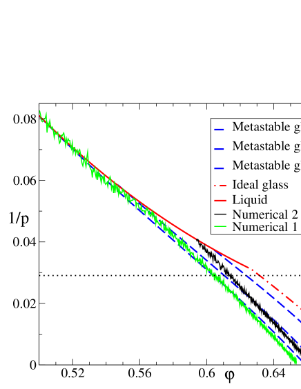
Figure 3: (Color online) Inverse reduced pressure, $\rho/(\beta P)$ as a function of the packing fraction $\varphi$ for a mixture with $r=1.4$ and $x=1$. Numerical data are obtained using two different protocols. In the first, compression is started at low density. In the second, compression is started from an equilibrated configuration at $\varphi=0.58$. The equation of state of different metastable glasses, corresponding to different $\Sigma_{j}$, are reported as dashed lines. The dot-dashed line is the pressure of the ideal glass, corresponding to $\Sigma_{j}=0$. A numerical estimate Berthier and Witten (2009) of the Kauzmann pressure, $p_{K}=34.4$, is reported as a dotted horizontal line.

Here we discuss in detail the behavior of pressure during compression in our numerical simulations. In figure 3 we report the evolution of the inverse reduced pressure during the first and second stages of compression (Numerical 1) for a mixture with $x=1$ and $r=1.4$. We observe, as in similar studies Donev et al. (2006); Skoge et al. (2006); Berthier and Witten (2009); Hermes and Dijkstra (2009), that the pressure follows the liquid equation of state up to some density, that for this system is around $\varphi\sim 0.56$. At this value of density, the relaxation time of the liquid becomes long enough that liquid relaxation is effectively frozen on the compression time scale used in this work and the system falls out of equilibrium. Although we did not measure relaxation time directly, this has been done in related works that confirmed the correctness of this statement Berthier and Witten (2009); Hermes and Dijkstra (2009); Foffi et al. (2003). Above this density, pressure increases faster and diverges on approaching jamming around $\varphi_{j}\sim 0.65$. The numerical equation of state is compared with that of a glass state corresponding to $\Sigma_{j}=1.5$. This is consistent with previous observations, that the configurational entropy is close to $1$ when the system falls out of equilibrium Angelani and Foffi (2007). In the same plot, we report the curve (Numerical 2) obtained starting the first stage from a carefully equilibrated liquid configuration of the same mixture at $\varphi=0.58$, kindly provided by L. Berthier (see Berthier and Witten (2009) for details on how this configuration was produced and equilibration was checked). In this case, since the relaxation time of the liquid at that density is already very long compared to our compression rate, the system falls immediately out of equilibrium and the pressure increases fast until jamming occurs at a higher density compared to the previous case. In our interpretation, this corresponds to a glassy state with lower $\Sigma_{j}$ (compare with the theoretical curve for $\Sigma_{j}\sim 1.2$). This is a nice confirmation of a prediction of the theory, that different glassy states jam at different density. Finally, we report, for the same system, the numerically extrapolated value of the ideal glass transition pressure, $p_{K}=34.4$, see Ref. Berthier and Witten (2009) for details of the careful extrapolation procedure. Again, this corresponds well (within 10$\%$) to the computed value $p_{K}=31.8$ from the theory, see figure 3. Note that this coincidence does not prove the existence of the Kauzmann transition, since on much larger time and length scales than the ones explored in these simulations, a crossover to a non mean-field behavior might happen. Still, the coincidence shows that, on the length and time scales explored by current numerical simulations, the full mean field phenomenology is observed, including the apparent extrapolation of Kauzmann transition. Whether this transition really exists remains a major open point of the field, that however does not affect the results presented here.

II Replica theory for multicomponent mixtures

Here we show in detail how to generalize the computation of Parisi and Zamponi (2008) to multicomponent mixtures. We will not repeat the discussion of Parisi and Zamponi (2008) but we only explain how to modify it for mixtures. Reading Appendix B and C and section VII of Parisi and Zamponi (2008) is necessary to follow the discussion.

We consider a multicomponent system in a (large) volume $V$ with partial densities $\rho_{\mu}=N_{\mu}/N$. The total density is $\rho=\sum_{\mu}\rho_{\mu}$ and we define $x_{\mu}=\rho_{\mu}/\rho$. Spheres of type $\mu$ have diameter $D_{\mu}$ and we define $D_{\mu\nu}=(D_{\mu}+D_{\nu})/2$. We denote by $\Omega_{d}=2\pi^{d/2}/\Gamma(d/2)$ the $d$-dimensional solid angle, and by $V_{d}(D)=\pi^{d/2}D^{d}/\Gamma(1+d/2)$ the volume of a $d$-dimensional sphere of diameter $D$. The hard sphere potential $\phi_{\mu\nu}(r)$ is infinite for $r<D_{\mu\nu}$ and zero otherwise: we denote $\chi_{\mu\nu}(r)=\exp[-\phi_{\mu\nu}(r)]$. $g_{\mu\nu}(r)$, as usual, is the $\mu$-$\nu$ pair correlation function Hansen and McDonald (1986). We will use the shorthand notations $g_{\mu\nu}\equiv g_{\mu\nu}(D_{\mu\nu})$ for the contact values of $g_{\mu\nu}(r)$, and $V_{d}^{\mu\nu}=V_{d}(D_{\mu\nu})$ for the volume of a sphere of diameter $D_{\mu\nu}$.

As discussed in Coluzzi et al. (1999), we assume that in the replicated liquid molecules are built of particles of the same type. This amounts to assume that in a glassy state particles of different type cannot easily exchange. However, as the diffusion constant is always finite in a glass, this assumption is wrong, since particles can exchange also within a state. This is all the more true in the liquid phase before the glass transition. Therefore, in order to correct this error, we will subtract the mixing entropy from the configurational entropy we will compute in the following, in order to obtain the correct physical result.

According to Coluzzi et al. (1999), to each molecule of the replicated liquid we can attach a label $\mu=1,\cdots,n$ according to the type of particles that build the molecule. We denote coordinates in a molecule by $\bar{x}=(x_{1},\cdots,x_{m})$. We have then to compute the free energy functional of a liquid made of $n$ species of molecules, with a single molecule density $\rho_{\mu}(\bar{x})$ and an interaction $\bar{\chi}_{\mu\nu}(\bar{x},\bar{y})=\prod_{a=1}^{m}\chi_{\mu\nu}(x_{a}-y_{a})$.

Effective liquid

We assume that the vibrations of the $m$ copies are described by a Gaussian distribution, corresponding to harmonic vibrations:

$$\rho_{\mu}(\bar{x})=\rho_{\mu}\int dX\prod_{a=1}^{m}\frac{e^{-\frac{(x_{a}-X)^{2}}{2A_{\mu}}}}{(\sqrt{2\pi A_{\mu}})^{d}}\ .$$ (3)

The widths $A_{\mu}$ are variational parameters and we will maximize the entropy with respect to them at the end. We choose a replica (say replica 1) as a reference and consider the vibrations of the other $m-1$ particles around the reference one. We want to construct an expansion assuming that $A_{\mu}$ is small. For $A_{\mu}=0$, the $m-1$ copies coincide with the reference one, and $\SS(m,\varphi)$ is given by the entropy $S(\varphi)$ of the non-replicated liquid plus the entropy of $m-1$ harmonic oscillators of spring constant $A_{\mu}$ (averaged over the concentration of the different species):

$$\SS^{(0)}(m,\varphi)=S(\varphi)+\sum_{\mu}x_{\mu}S_{harm}(m,A_{\mu})\ .$$ (4)

The harmonic part of the entropy is computed straightforwardly from the term $\sum_{\mu}\int d\bar{x}\rho_{\mu}(\bar{x})[1-\log\rho_{\mu}(\bar{x})]$ in the free energy functional, see section V of Parisi and Zamponi (2008), where the function $S_{harm}(m,A)$ is also defined.

A first order approximation is obtained by considering the effective two-body interaction induced on the particles of replica 1 by the coupling to the $m-1$ copies. This can be justified on the basis of a diagrammatic expansion following the derivation in Appendix B of Parisi and Zamponi (2008), see also Stoessel and Wolynes (1984). It is possible to show Hansen and McDonald (1986) that the diagrammatic expansion of the free energy functional for a multicomponent liquid is the same as the one of a simple liquid, provided a label $\mu_{i}$ is attached to each vertex $i$, and in such a labeled diagram $\rho_{\mu_{i}}(x_{i})$ is placed on each vertex, $\chi_{\mu_{i}\mu_{j}}(x_{i}-x_{j})$ on each link, and a sum over $\mu_{i}$ is performed in addition to the integration over $x_{i}$. The same is true for the molecular liquid. Hence, the treatment of diagrams performed in Appendix B of Parisi and Zamponi (2008) can be repeated exactly for a mixture, taking into account the presence of the additional labels. This is straightforward and leads to the introduction of effective potentials that now depend on the type of particles involved. In particular, one obtains:

$$\begin{split}e^{-\phi^{eff}_{\mu\nu}(x_{1}-y_{1})}&=\int dx_{2}\cdots dx_{m}dy_{2}\cdots dy_{m}\rho_{\mu}(\bar{x})\,\rho_{\nu}(\bar{y})\prod_{a=1}^{m}e^{-\phi_{\mu\nu}(x_{a}-y_{a})}\\ &\equiv e^{-\phi_{\mu\nu}(x_{1}-y_{1})}[1+Q_{\mu\nu}(x_{1}-y_{1})]\ .\end{split}$$ (5)

A first order approximation to $\SS(m,\varphi)$ is then obtained by substituting to the entropy $S(\varphi)$ of the simple hard sphere mixture the free energy of a liquid of particles interacting via the potential $\phi^{eff}_{\mu\nu}(r)$:

$$\SS^{(1)}(m,\varphi)=-F[\varphi,\phi^{eff}_{\mu\nu}(r)]+\sum_{\mu}x_{\mu}S_{harm}(m,A_{\mu})\ .$$ (6)

It is now evident that we can obtain better approximations of the true function $\SS(m,\varphi)$ by considering also the three body interactions induced on particles of the replica 1, and so on. Here, for simplicity, we will limit ourselves to consider the two-body interactions. To the same approximation, the pair correlation function $g_{\mu\nu}(r)$ of the system is given by the correlation of the effective liquid of particles interacting via $\phi_{\mu\nu}(r)$. For small $A_{\mu}$, $\phi^{eff}_{\mu\nu}$ is close to $\phi_{\mu\nu}$ and the free energy in Eq. (6) can be computed in perturbation theory around the normal liquid Hansen and McDonald (1986), which is taken as an input for the calculation of the properties of the glass.

Small cage expansion

Now we follow the discussion in section VII of Parisi and Zamponi (2008) to compute the entropy of the effective liquid. We assume that the cage radius is small, therefore $Q_{\mu\nu}$ can be considered as a perturbation, and one has $\phi^{eff}_{\mu\nu}(r)\sim\phi_{\mu\nu}(r)-Q_{\mu\nu}(r)$. Using the general relation Hansen and McDonald (1986)

$$\frac{\delta F[\varphi,\phi_{\mu\nu}(r)]}{\delta\phi_{\mu\nu}(r)}=\frac{\rho_{\mu}\rho_{\nu}}{2\rho}g_{\mu\nu}(r)\ ,$$ (7)

we obtain

$$-F[\varphi,\phi^{eff}_{\mu\nu}(r)]\sim S(\varphi)+\sum_{\mu,\nu}\frac{\rho_{\mu}\rho_{\nu}}{2\rho}\int drg_{\mu\nu}(r)Q_{\mu\nu}(r)\ ,$$ (8)

where $S(\varphi)=-F[\varphi,\phi_{\mu\nu}(r)]$ is the entropy of the liquid. The function $Q_{\mu\nu}(r)$ is different from zero only for $r-D_{\mu\nu}\sim O(\sqrt{A_{\mu}+A_{\nu}})$. If $\sqrt{A_{\mu}+A_{\nu}}\ll D_{\mu\nu}$ we can assume that the function $g_{\mu\nu}(r)$ is essentially constant on the scale $\sqrt{A_{\mu}+A_{\nu}}$, then $g_{\mu\nu}(r)\sim g_{\mu\nu}\chi_{\mu\nu}(r)$ for $r-D_{\mu\nu}\sim O(\sqrt{A_{\mu}+A_{\nu}})$, and

$$\begin{split}\int drg_{\mu\nu}(r)Q_{\mu\nu}(r)\sim g_{\mu\nu}\int dr\chi_{\mu\nu}(r)Q_{\mu\nu}(r)\ .\end{split}$$ (9)

To compute the previous expression, all the considerations of Appendix C of Parisi and Zamponi (2008) can be repeated. Instead of a single function $Q(r)$, one has $Q_{\mu\nu}(r)$, and in the two Gaussians one has $A_{\mu}$ and $A_{\nu}$ instead of $A$. At the very beginning of the discussion, then, one finds that it is enough to replace $2A\rightarrow A_{\mu}+A_{\nu}$ and follow the same steps. We obtain

$$\int dr\chi_{\mu\nu}(r)Q_{\mu\nu}(r)=\frac{d\,V_{d}^{\mu\nu}}{D_{\mu\nu}}\sqrt{2(A_{\mu}+A_{\nu})}\,Q_{0}(m)\ .$$ (10)

where $Q_{0}(m)$ is defined in Appendix C of Parisi and Zamponi (2008).

Putting all together, we find the final result

$$\begin{split}\SS(m,\varphi;\{A_{\mu}\})=\sum_{\mu}x_{\mu}S_{harm}(m,A_{\mu})+S(\varphi)+\sum_{\mu,\nu}\frac{\rho_{\mu}\rho_{\nu}}{2\rho}g_{\mu\nu}\frac{d\,V_{d}^{\mu\nu}}{D_{\mu\nu}}\sqrt{2(A_{\mu}+A_{\nu})}\,Q_{0}(m)\end{split}$$ (11)

This expression generalizes the result of section VII of Parisi and Zamponi (2008) to multicomponent mixtures; it has to be optimized over all the $A_{\mu}$ to get the replicated entropy $\SS(m,\varphi)$.

Replicated free energy for binary mixtures

The optimization with respect to $A_{\mu}$ leads to $n$ coupled equations that are not easy to solve in general. Therefore in the following we focus on the case of binary mixtures that is of interest here.

For convenience we denote $A_{A}=A$ and $A_{B}=B$ the cage radii of the two species. We then obtain

$$\begin{split}\frac{\partial\SS(m,\varphi;A,B)}{\partial A}&=\frac{\rho_{A}^{2}g_{AA}V_{d}^{AA}d}{2\rho D_{AA}}\frac{Q_{0}(m)}{\sqrt{A}}+\frac{\rho_{A}\rho_{B}g_{AB}V_{d}^{AB}d}{\rho D_{AB}}\frac{Q_{0}(m)}{\sqrt{2(A+B)}}-x_{A}\frac{d(1-m)}{2A}=0\\ \frac{\partial\SS(m,\varphi;A,B)}{\partial B}&=\frac{\rho_{B}^{2}g_{BB}V_{d}^{BB}d}{2\rho D_{BB}}\frac{Q_{0}(m)}{\sqrt{B}}+\frac{\rho_{A}\rho_{B}g_{AB}V_{d}^{AB}d}{\rho D_{AB}}\frac{Q_{0}(m)}{\sqrt{2(A+B)}}-x_{B}\frac{d(1-m)}{2B}=0\\ \end{split}$$ (12)

Defining $\delta=B/A$, $x=\rho_{A}/\rho_{B}$ and $r=D_{A}/D_{B}$, we obtain the following equation for $\delta$:

$$\begin{split}&x\,r^{d-1}\,g_{AA}-\sqrt{\delta}\,g_{BB}+\frac{\sqrt{2}(1-x\delta)}{\sqrt{(1+\delta)}}\left(\frac{1+r}{2}\right)^{d-1}g_{AB}=0\ ,\end{split}$$ (13)

and from its solution we obtain the optimal values of $A$ and $B=\delta\,A$:

$$\begin{split}&\sqrt{A^{\star}(\delta)}=\frac{1-m}{2Q_{0}(m)}\frac{\left\langle D^{d}\right\rangle(1+x)}{2^{d}\,\varphi\,\Gamma}\\ &\Gamma=\frac{1}{2}xg_{AA}D_{AA}^{d-1}+g_{AB}\frac{D_{AB}^{d-1}}{\sqrt{2(1+\delta)}}\end{split}$$ (14)

where the packing fraction is $\varphi=\rho_{A}V_{d}(D_{A})+\rho_{B}V_{d}(D_{B})$ and $\left\langle D^{p}\right\rangle=\sum_{\mu}x_{\mu}D_{\mu}^{p}$. Substituting these in $\SS(m,\varphi;A,B)$, we finally get

$$\begin{split}&\SS(m,\varphi)=S(\varphi)-\frac{d}{2}(1-m-\log m)-\frac{d}{2}(1-m)\log(2\pi A^{\star})-\frac{d}{2}\frac{1}{1+x}(1-m)\log(\delta)+\frac{2^{d}d\,\varphi}{\left\langle D^{d}\right\rangle}\frac{Q_{0}(m)\sqrt{A^{\star}}\Delta}{(1+x)^{2}}\\ &\Delta=x^{2}g_{AA}D_{AA}^{d-1}+xg_{AB}D_{AB}^{d-1}\sqrt{2(1+\delta)}+g_{BB}D_{BB}^{d-1}\sqrt{\delta}\end{split}$$ (15)

From this expression one can compute the complexity using Eq. (2) Parisi and Zamponi (2008); here it is not useful to report the complete expression. However, it is interesting to report the following explicit expressions:

$$\begin{split}\Sigma_{j}(\varphi)&=\lim_{m\rightarrow 0}\Sigma(m,\varphi)=S(\varphi)-d\log\left(\frac{\sqrt{2}\left<D^{d}\right>(1+x)}{2^{d}\varphi\Gamma}\right)-\frac{d}{2}\frac{1}{1+x}\log\delta+\frac{d}{2}\ ,\\ \Sigma_{eq}(\varphi)&=\Sigma(1,\varphi)=S(\varphi)-d\log\left[\sqrt{\frac{\pi}{2}}\frac{\left<D^{d}\right>(1+x)}{2^{d}K\varphi\Gamma}\right]-\frac{d}{2}\frac{1}{1+x}\log\delta\end{split}$$ (16)

with $K=-Q^{\prime}(1)=0.638\ldots$, see Parisi and Zamponi (2008) for details. From the latter expressions one can compute the Kauzmann density $\varphi_{K}$ which is the solution of $\Sigma_{eq}(\varphi)=0$, and the Glass Close Packing density $\varphi_{GCP}$ which is the solution of $\Sigma_{j}(\varphi)=0$ Parisi and Zamponi (2008). More generally, given a set of metastable glasses of complexity $\Sigma_{j}$, under the so-called isocomplexity assumption Parisi and Zamponi (2008), one can compute their jamming density as the solution of $\Sigma_{j}(\varphi)=\Sigma_{j}$. The results of this computation for binary mixtures are discussed in the main text. One should keep in mind that, as discussed above, Eqs. (16) incorrectly includes the mixing entropy (coming from the $S(\varphi)$ term). This has to be subtracted in order to get the correct physical result.

Coordination numbers

Here we show how to compute the partial coordination numbers. The technical part of the computation follow closely the derivation in Parisi and Zamponi (2008), hence the only nontrivial point is to add indices corresponding to particle types. As discussed in section VII.C.3 of Parisi and Zamponi (2008), the integral of the glass correlation function, $\widetilde{g}^{\mu\nu}(r)$, on a shell $D_{\mu\nu}\leq r\leq D_{\mu\nu}+O(\sqrt{\varphi_{j}-\varphi})$ gives the number of particles of type $\nu$ that are in contact with a given particle of type $\mu$ for $\varphi\rightarrow\varphi_{j}$. A straightforward generalization of the derivation of section VII.C.2 of Parisi and Zamponi (2008) shows that, at the leading order close to contact, $\widetilde{g}_{\mu\nu}(r)=g_{\mu\nu}(r)[1+Q_{\mu\nu}(r)]\sim g_{\mu\nu}[1+Q_{\mu\nu}(r)]$. Then one obtains

$$\begin{split}z_{\mu\nu}=\Omega_{d}\rho_{\nu}D_{\mu\nu}^{d-1}g_{\mu\nu}\int_{D_{\mu\nu}}^{D_{\mu\nu}+O(\sqrt{(A_{\mu}+A_{\nu})/2})}dr\,[1+Q_{\mu\nu}(r)]\ .\end{split}$$ (17)

In the limit $\varphi\rightarrow\varphi_{j}$, one has $A_{\mu}\propto m\rightarrow 0$ and the integral of $Q_{\mu\nu}(r)$ can be easily evaluated Parisi and Zamponi (2008). The result is

$$\begin{split}z_{\mu\nu}=\Omega_{d}\rho_{\nu}D_{\mu\nu}^{d-1}g_{\mu\nu}\sqrt{2(a_{\mu}+a_{\nu})}\end{split}$$ (18)

where $a_{\mu}=\lim_{m\rightarrow 0}A_{\mu}\left(\frac{Q_{0}(m)}{1-m}\right)^{2}$.

In the explicit case of binary mixtures, note that the equation (13) for $\delta$ does not depend on $m$. Using also Eq. (14), we obtain

$$\begin{cases}&z_{AA}=xD_{AA}^{d-1}g_{AA}\frac{d}{\Gamma}\\ &z_{BB}=D_{BB}^{d-1}g_{BB}\sqrt{\delta}\frac{d}{\Gamma}\\ &z_{AB}=D_{AB}^{d-1}g_{AB}\sqrt{\frac{1+\delta}{2}}\frac{d}{\Gamma}\\ &z_{BA}=xD_{AB}^{d-1}g_{AB}\sqrt{\frac{1+\delta}{2}}\frac{d}{\Gamma}\end{cases}$$ (19)

Note that it is possible to show, using the definitions of $\delta$ and $\Gamma$, that the average total coordination $z=\sum_{\mu\nu}x_{\mu}z_{\mu\nu}=6$, i.e. the packings are predicted to be isostatic irrespective of the mixture composition.

Equation of state for liquid hard sphere mixtures

We used a generalization of the Carnahan-Starling equation of state, which is defined by the following relation for the contact value of the radial distribution function Santos et al. (2005):

$$\begin{split}&g_{\mu\nu}(\varphi)=\frac{1}{1-\varphi}+\left(g_{pure}(\varphi)-\frac{1}{1-\varphi}\right)\frac{\left<D^{d-1}\right>D_{\mu\mu}D_{\nu\nu}}{\left<D^{d}\right>D_{\mu\nu}}\ ,\end{split}$$ (20)

where $g_{pure}(\varphi)$ is the contact value of $g(r)$ for the pure system, given by the standard Carnahan-Starling equation Hansen and McDonald (1986). The pressure is then given by the exact relation

$$p(\varphi)=\frac{\beta P}{\rho}=1+\frac{2^{d-1}}{\left<D^{d}\right>}\varphi\sum_{\mu\nu}x_{\mu}x_{\nu}D^{d}_{\mu\nu}g_{\mu\nu}=-\varphi\frac{\partial S(\varphi)}{\partial\varphi}$$ (21)

Integrating this expression one obtains the entropy $S(\varphi)$. The additive integration constant is fixed by the condition that, for $\varphi\rightarrow 0$, the entropy tends to the ideal gas value $S(\varphi)=1-\log\rho-\sum_{\mu}x_{\mu}\log x_{\mu}$. This expression includes the mixing entropy that must be subtracted before substituting $S(\varphi)$ into Eqs. (16).

References

- Torquato et al. (2000) S. Torquato, T. M. Truskett, and P. G. Debenedetti, Phys. Rev. Lett. 84, 2064 (2000).
- Scott and Kilgour (1969) G. D. Scott and D. M. Kilgour, Brit. J. Appl. Phys. (J. Phys. D) 2, 863 (1969).
- Bennett (1972) C. H. Bennett, J. Appl. Phys. 43, 2727 (1972).
- Lubachevsky and Stillinger (1990) B. D. Lubachevsky and F. H. Stillinger, J. Stat. Phys. 60, 561 (1990).
- Donev et al. (2006) A. Donev, F. H. Stillinger, and S. Torquato, Physical Review Letters 96, 225502 (pages 4) (2006).
- Jodrey and Tory (1985) W. S. Jodrey and E. M. Tory, Phys. Rev. A 32, 2347 (1985).
- Clarke and Jónsson (1993) A. S. Clarke and H. Jónsson, Phys. Rev. E 47, 3975 (1993).
- O’Hern et al. (2002) C. S. O’Hern, S. A. Langer, A. J. Liu, and S. R. Nagel, Phys. Rev. Lett. 88, 075507 (2002).
- Lochmann et al. (2006) K. Lochmann, A. Anikeenko, A. Elsner, N. Medvedev, and D. Stoyan, The European Physical Journal B 53, 67 (2006).
- Kamien and Liu (2007) R. D. Kamien and A. J. Liu, Physical Review Letters 99, 155501 (pages 4) (2007).
- Dodds (1975) J. Dodds, Nature 256, 187 (1975).
- Dodds (1980) J. Dodds, Journal of Colloid and Interface Science 77, 317 (1980).
- Ouchiyama and Tanaka (1981) N. Ouchiyama and T. Tanaka, Industrial & Engineering Chemistry Fundamentals 20, 66 (1981).
- Woodcock and Angell (1981) L. V. Woodcock and C. A. Angell, Phys. Rev. Lett. 47, 1129 (1981).
- Stoessel and Wolynes (1984) J. P. Stoessel and P. G. Wolynes, The Journal of Chemical Physics 80, 4502 (1984).
- Speedy (1998) R. J. Speedy, Mol. Phys. 95, 169 (1998).
- Cardenas et al. (1998) M. Cardenas, S. Franz, and G. Parisi, Journal of Physics A: Mathematical and General 31, L163 (1998).
- Parisi and Zamponi (2005) G. Parisi and F. Zamponi, The Journal of Chemical Physics 123, 144501 (pages 12) (2005).
- Krzakala and Kurchan (2007) F. Krzakala and J. Kurchan, Physical Review E (Statistical, Nonlinear, and Soft Matter Physics) 76, 021122 (pages 13) (2007).
- Parisi and Zamponi (2008) G. Parisi and F. Zamponi (2008), eprint arXiv:0802.2180.
- Santen and Krauth (2000) L. Santen and W. Krauth, Nature 405, 550 (2000).
- Berthier and Witten (2008) L. Berthier and T. Witten (2008), eprint arXiv.org: 0810.4405.
- Berthier and Witten (2009) L. Berthier and T. Witten, The glass transition of dense fluids of hard and compressible spheres (2009), eprint arXiv.org: 0903.1934.
- Hansen and McDonald (1986) J.-P. Hansen and I. R. McDonald, Theory of simple liquids (Academic Press, London, 1986).
- Mézard and Parisi (1999) M. Mézard and G. Parisi, The Journal of Chemical Physics 111, 1076 (1999).
- Mézard et al. (1987) M. Mézard, G. Parisi, and M. A. Virasoro, Spin glass theory and beyond (World Scientific, Singapore, 1987).
- Monasson (1995) R. Monasson, Phys. Rev. Lett. 75, 2847 (1995).
- Coluzzi et al. (1999) B. Coluzzi, M. Mézard, G. Parisi, and P. Verrocchio, The Journal of Chemical Physics 111, 9039 (1999).
- Goldstein (1969) M. Goldstein, The Journal of Chemical Physics 51, 3728 (1969).
- Yerazunis et al. (1965) S. Yerazunis, S. Cornell, and B. Wintner, Nature 207, 835 (1965).
- Pinson et al. (1998) D. Pinson, R. P. Zou, A. B. Yu, P. Zulli, and M. J. McCarthy, Journal of Physics D: Applied Physics 31, 457 (1998).
- Santos et al. (2005) A. Santos, M. L. de Haro, and S. B. Yuste, The Journal of Chemical Physics 122, 024514 (pages 15) (2005).
- Donev et al. (2005) A. Donev, S. Torquato, and F. H. Stillinger, Journal of Computational Physics 202, 737 (2005).
- Donev and Torquato (2005) A. Donev and S. Torquato, Home Page (2005), URL http://cherrypit.princeton.edu/donev/Packing/PackLSD/Instruct%ions.html.
- Skoge et al. (2006) M. Skoge, A. Donev, F. H. Stillinger, and S. Torquato, Physical Review E (Statistical, Nonlinear, and Soft Matter Physics) 74, 041127 (pages 11) (2006).
- Götze and Voigtmann (2003) W. Götze and T. Voigtmann, Phys. Rev. E 67, 021502 (2003).
- Foffi et al. (2003) G. Foffi, W. Götze, F. Sciortino, P. Tartaglia, and T. Voigtmann, Phys. Rev. Lett. 91, 085701 (2003).
- Hermes and Dijkstra (2009) M. Hermes and M. Dijkstra, Random close packing of polydisperse hard spheres (2009), eprint arXiv.org: 0903.4075.
- Angelani and Foffi (2007) L. Angelani and G. Foffi, J. Phys.: Condens. Matter 19, 256207 (2007).