Threshold Resummation Effects in Neutral Higgs Boson Production by Bottom Quark Fusion at the CERN Large Hadron Collider

Abstract

We investigate the QCD effects in the production of neutral Higgs bosons via bottom quark fusion in both the standard model and the minimal supersymmetric standard model at the CERN Large Hadron Collider. We include the next-to-leading order (NLO) QCD corrections (including supersymmetric QCD) and the threshold resummation effects. We use the soft-collinear effective theory to resum the large logarithms near threshold from soft gluon emission. Our results show that the resummation effects can enhance the total cross sections by about 5% compared with the NLO results.

I INTRODUCTION

The understanding of Electroweak Symmetry Breaking (EWSB) plays a key role in current research of high energy physics. In the Standard Model (SM), a complex scalar doublet is responsible for the generation of gauge bosons and fermions masses by the Higgs mechanism. One neutral Higgs boson ($h$) survives after EWSB, which is the last elementary particle yet to be found in the SM. Direct searches at LEP$2$ set a lower bound on the SM Higgs boson mass $m_{h}>114.4$ GeV (at 95%CL) Barate:2003sz , while electroweak precision measurements prefer a light Higgs boson of $m_{h}\lesssim 180$ GeV Alcaraz:2007ri .

In the most popular extensions of the SM, e.g., the Minimal Supersymmetric Standard Model (MSSM), two Higgs doublets are required in order to preserve supersymmetry (SUSY) and anomaly cancellation. In the MSSM, the Higgs sector consists of five physical Higgs bosons: the neutral CP-even ones $h$ and $H$, the neutral CP-odd one $A$, and the charged ones $H^{\pm}$. The lightest one $h$ behaves like the SM one in the decoupling limit $(M_{A}\gg M_{Z^{0}})$. Its mass is constrained by a theoretical upper bound of $M_{h}\lesssim(130-140)$ GeV when taking into account the radiative corrections massh0 . At lowest order, two parameters are required to describe the MSSM Higgs sector, which are generally chosen to be $m_{A}$ and $\tan\beta=v_{2}/v_{1}$, the ratio of the two vacuum expectation values.

For large value of $\tan\beta$, the bottom-Higgs Yukawa coupling can be considerably enhanced, thus Higgs production associated with bottom quarks may be quite important in MSSM. There are two approaches for calculating cross sections involving bottom quarks: the four flavor number scheme (4FNS) and five flavor number scheme (5FNS) Dawson:2005vi . In the 4FNS, there are no initial state bottom quarks. Due to non zero of bottom quark mass, large logarithms may appear from gluon splitting, hence transverse momentum ($p_{T}$) and pseudo rapidity cuts on final state bottom quarks are needed to eliminate these large logarithms. In the 5FNS, initial state bottom quarks are treated as massless, and by introducing a perturbatively defined bottom quark parton distribution function (PDF), large logarithms are resummed through the DGLAP evolution equation. Except for $q\bar{q}\rightarrow b\bar{b}h$, the other relevant production mechanisms depend on the final state being observed Campbell:2004pu . For inclusive Higgs production without bottom tagged in final state, the lowest order process is $gg\rightarrow(b\bar{b})h$ ($b\bar{b}\rightarrow h$) in 4FNS (5FNS) Dicus:1998hs . However, if at least one high-$p_{T}$ $b$ quark is required to be observed, the leading partonic process is $gg\rightarrow b(\bar{b})h$ ($gb\rightarrow bh$) in 4FNS (5FNS) gbbh , and if two high-$p_{T}$ $b$ quarks are required, the leading subprocess is $gg\rightarrow b\bar{b}h$ ggbbh and can only be calculated in 4FNS. There are extensive comparison between 4FNS and 5FNS and good agreement has been found between the two schemes within theoretical uncertainties Campbell:2004pu ; comparison .

In recent years much effort has been made to the precise prediction of the inclusive cross section for Higgs boson production via bottom quark fusion, with neither bottom quark detected $b\bar{b}\rightarrow h$. The next-to-leading order (NLO) QCD corrections Dicus:1998hs ; Balazs:1998sb ; Maltoni:2003pn and the next-to-next-to-leading order (NNLO) QCD corrections Harlander:2003ai to this process have been calculated. Also the SUSY QCD and SUSY electroweak corrections to this process have been studied Dittmaier:2006cz .

When the hard scattering process involves two very different scale, the fixed order perturbation expansion contains large logarithms of scale ratio. These terms might spoil the reliability of the perturbation expansion and need to be resummed to all orders Sterman:1986aj ; Catani:1989ne . In general, the large logarithms mentioned above can appear when the Higgs boson in the final state has small transverse momentum or is produced near threshold. The transverse momentum resummation were calculated in Refs. Field:2004nc ; Belyaev:2005bs , and the threshold resummation effects are considered Ravindran:2006cg ; Kidonakis:2007ww with the conventional method Sterman:1986aj ; Catani:1989ne , where partial next-next-next-to-leading-order (NNNLO) results are obtained by expanding the resummed cross sections. In this paper, we will further study the complete next-to-leading-logarthmic (NLL) threshold resummation effects on the production cross sections using soft-collinear effective theory (SCET) scet in both the SM and MSSM at the CERN Large Hadron Collider (LHC).

The paper is organized as follows: In Sec. II and III we present the analytic results at fixed order. In Sec. IV we use SCET to derive the resummed formula for the cross sections. In Sec. V the numerical results are presented and discussed. Sec. VI contains a brief summary and conclusions.

II THE LEADING ORDER RESULTS

We consider the inclusive process $A(p_{a})+B(p_{b})\rightarrow H_{i}(q)+X$, where A and B are the incoming hadrons with momenta $p_{a}$ and $p_{b}$, $H_{i}=\{h,H,A\}$ are neutral CP-even or CP-odd Higgs bosons, with momentum $q$, and X is arbitrary hadronic state.

At hadron colliders the total cross sections can be factorized into the convolution of the partonic cross sections with appropriate PDFs:

$$\sigma(M^{2}_{i},s)=\sum_{a,b}\int^{1}_{\tau}~{}dx_{a}\int^{1}_{\tau/x_{a}}~{}dx_{b}~{}f_{a/A}(x_{a},\mu_{f})f_{b/B}(x_{b},\mu_{f})\hat{\sigma}_{ab}(z,M^{2}_{i};\alpha_{s}(\mu^{2}_{r}),\mu^{2}_{r},\mu^{2}_{f}),$$ (1)

where $\hat{\sigma}_{ab}$ is the cross section for the partonic subprocess $a(\hat{p}_{a})+b(\hat{p}_{b})\rightarrow H_{i}(q)+X$, $\hat{p}_{a}$ and $\hat{p}_{b}$ are the momentum of the incoming partons $a,b$. The momentum fractions $x_{a}$ and $x_{b}$ are defined by $x_{a(b)}=\hat{p}_{a(b)}/p_{a(b)}$, $M_{i}$ is the mass of the final state Higgs boson, $\tau=M^{2}_{i}/s$, and the scaling variable $z=M^{2}_{i}/\hat{s}$, where $\hat{s}=(\hat{p}_{a}+\hat{p}_{b})^{2}$. $f_{p/H}(x,\mu_{f})$ is the parton distribution function which describes the probability of finding a parton $p$ with momentum fraction $x$ inside the hadron $H$ at factorization scale $\mu_{f}$. The sum is over all possible initial partons.

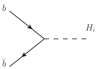
Figure 1: Leading-order Feynman diagrams for $b\bar{b}\rightarrow H_{i}$

The leading-order (LO) Feynman diagrams is shown in Fig. 1, and its LO amplitude in $n=4-2\epsilon$ dimension is

$$i\mathcal{M}_{B}=\mu^{\epsilon}_{r}Y_{b}\kappa_{i}\bar{v}(p_{b})\Gamma^{(i)}u(p_{a}),$$ (2)

where $Y_{b}\equiv-igm_{b}/(2m_{W})$ is the SM coupling of Higgs boson to bottom quark, and $\mu_{r}$ is a mass parameter introduced to keep the coupling constant $g$ dimensionless. Furthermore, we have $\Gamma^{(h,H)}=1$ for scalar ($h,H$) production and $\Gamma^{(A)}=\gamma^{5}$ for pseudoscalar ($A$) production. The explicit expressions for $\kappa_{i}$ are:

$$\kappa_{h}=-\frac{\sin\alpha}{\cos\beta},\ \ \ \ \ \kappa_{H}=\frac{\cos\alpha}{\cos\beta},\ \ \ \ \ \kappa_{A}=-i\tan\beta.$$

Here $\alpha$ is the mixing angle between the weak and the mass eigenstates of the neutral CP-even Higgs boson sector.

The LO partonic cross sections are given by

$$\hat{\sigma}_{B}=\frac{1}{2\hat{s}}\int~{}\overline{\sum}|\mathcal{M}_{B}|^{2}dPS^{(1)}=\hat{\sigma}_{0}\delta(1-z),$$ (3)

where $\overline{\sum}$ indicates the summation over final states and the average over initial states, $\int dPS^{(1)}$ represents the phase space integration and $\hat{\sigma}_{0}=\mu^{2\epsilon}_{r}\pi|Y_{b}\kappa_{i}|^{2}/(6\hat{s})$.

III NEXT-TO-LEADING ORDER CALCULATIONS

The NLO QCD and SUSY QCD correctons to this process have been studied in Dabelstein:1995js ; Dicus:1998hs ; Maltoni:2003pn ; Harlander:2003ai ; Dittmaier:2006cz , but we recalculate it here to check the relevant results in the previous literatures and make our paper self-contained. At NLO, the QCD and SUSY QCD corrections consist of the following contributions: the exchange of virtual gluon or gluino and the corresponding renormalization counterterms, the real gluon emission subprocesses, the gluon initiated subprocesses, and the contributions of Altarelli-Parisi(A-P) splitting functions. In the following, we will calculate these contributions separately. We use dimensional regularization (DREG) in $n=4-2\epsilon$ dimensions to regulate all divergences, and adopt $\overline{\rm MS}$ renormalization and factorization scheme to remove the ultraviolet (UV) and infrared (IR) (including soft and collinear) divergences of QCD corrections, while SUSY QCD corrections are renormalized in on-shell scheme onmass .

III.1 Virtual corrections

The amplitude corresponding to virtual gluons exchange is given by

$$\mathcal{M}^{\rm QCD}_{V}=\mathcal{M}_{B}\frac{\alpha_{s}}{4\pi}C_{F}\left(\frac{4\pi\mu^{2}_{r}}{M^{2}_{i}}\right)^{\epsilon}\frac{\Gamma(1-\epsilon)}{\Gamma(1-2\epsilon)}\left(-\frac{2}{\epsilon^{2}_{\rm IR}}+\frac{3}{\epsilon_{\rm UV}}-\frac{3}{\epsilon_{\rm IR}}+\frac{2}{3}\pi^{2}-2\right),$$ (4)

where $C_{F}=4/3$ is the $SU(3)$ color factor. The above amplitude contains both UV and IR divergence. The renormalized QCD amplitude can be written as

$$\widetilde{\mathcal{M}}^{\rm QCD}_{V}=\mathcal{M}^{\rm QCD}_{V}+\frac{\delta m^{\rm QCD}_{b}}{m_{b}}\mathcal{M}_{B},$$ (5)

with Braaten:1980yq

$$\frac{\delta m^{\rm QCD}_{b}}{m_{b}}=-C_{F}\frac{\alpha_{s}}{4\pi}\frac{(4\pi)^{\epsilon}\Gamma(1-\epsilon)}{\Gamma(1-2\epsilon)}\frac{3}{\epsilon_{\rm UV}}.$$ (6)

The amplitude corresponding to virtual gluino and squark exchange is given by

$$\mathcal{M}^{\rm SUSY}_{V}=\mathcal{M}_{B}F^{(i)}.$$ (7)

Here $F^{(i)}$ $(i=h,H,A)$ are the SUSY form factors:

$$F^{(h,H)} = \frac{i}{Y_{b}\kappa_{h,H}}\frac{\alpha_{s}}{4\pi}C_{F}m_{\tilde{g}}\left[\sin 2\theta_{\tilde{b}}\left(G^{(h,H)}_{11}C_{0}(1,1)-G^{(h,H)}_{22}C_{0}(2,2)\right)\right.$$ (8)

$$\left.+\cos 2\theta_{\tilde{b}}\left(G^{(h,H)}_{12}C_{0}(1,2)+G^{(h,H)}_{21}C_{0}(2,1)\right)\right],$$

$$F^{(A)}=\frac{i}{Y_{b}\kappa_{A}}\frac{\alpha_{s}}{4\pi}C_{F}m_{\tilde{g}}\left(G^{(A)}_{12}C_{0}(1,2)-G^{(A)}_{21}C_{0}(2,1)\right),$$ (9)

where $C_{0}(i,j)$ are the usual Passarino-Veltman three-point functiondenner

$$C_{0}(i,j)\equiv C_{0}(m^{2}_{b},\hat{s},m^{2}_{b},m^{2}_{\tilde{g}},m^{2}_{\tilde{b}_{i}},m^{2}_{\tilde{b}_{j}}).$$ (10)

$iG^{(i)}_{lm}$ are the couplings between Higgs boson and sbottom mass eigenstates, which are given in the appendix. $m_{\tilde{b}_{1,2}}$ are the sbottom masses, $m_{\tilde{g}}$ is the gluino mass, and $R^{\tilde{b}}$ is a $2\times 2$ matrix defined to rotate the sbottom current eigenstates into the mass eigenstates:

$$\left(\begin{array}[]{c}\tilde{b}_{1}\\ \tilde{b}_{2}\end{array}\right)=R^{\tilde{b}}\left(\begin{array}[]{c}\tilde{b}_{L}\\ \tilde{b}_{R}\end{array}\right),\ \ \ \ \ R^{\tilde{b}}=\left(\begin{array}[]{cc}\cos\theta_{\tilde{b}}&\sin\theta_{\tilde{b}}\\ -\sin\theta_{\tilde{b}}&\cos\theta_{\tilde{b}}\end{array}\right),$$ (11)

with $0\leq\theta_{\tilde{b}}<\pi$ by convention. Correspondingly, the mass eigenvalues $m_{\tilde{b}_{1}}$ and $m_{\tilde{b}_{2}}$ (with $m_{\tilde{b}_{1}}\leq m_{\tilde{b}_{2}}$) are given by

$$\left(\begin{array}[]{cc}m_{\tilde{b}_{1}}^{2}&0\\ 0&m_{\tilde{b}_{2}}^{2}\end{array}\right)=R^{\tilde{b}}M_{\tilde{b}}^{2}(R^{\tilde{b}})^{\dagger},\ \ \ \ \ M_{\tilde{b}}^{2}=\left(\begin{array}[]{cc}m_{\tilde{b}_{L}}^{2}&X_{b}m_{b}\\ X_{b}m_{b}&m_{\tilde{b}_{R}}^{2}\end{array}\right),$$ (16)

with

$$m^{2}_{\tilde{b}_{L}} = M^{2}_{\tilde{Q}}+m_{b}^{2}+m_{Z}^{2}\cos 2\beta C_{bL},$$

$$m^{2}_{\tilde{b}_{R}} = M^{2}_{\tilde{D}}+m_{b}^{2}-m_{Z}^{2}\cos 2\beta C_{bR},$$

$$X_{b} = A_{b}-\mu\tan\beta.$$ (17)

where $C_{bL}=-1/2+\sin^{2}\theta_{W}/3$, $C_{bR}=\sin^{2}\theta_{W}/3$, and $M_{\tilde{b}}^{2}$ is the sbottom mass matrix. $M_{\tilde{Q},\tilde{D}}$ are soft SUSY-breaking parameters, $A_{b}$ is the trilinear Higgs-sbottom coupling, and $\mu$ is the Higgsino mass parameter.

The renormalized SUSY QCD amplitude is

$$\widetilde{\mathcal{M}}^{\rm SUSY}_{V}=\mathcal{M}^{\rm SUSY}_{V}+\left(\frac{\delta m^{\rm SUSY}_{b}}{m_{b}}+\frac{1}{2}(\delta Z_{bL}+\delta Z_{bR})\right)\mathcal{M}_{B},$$ (18)

and the renormalization constants in the on-shell scheme are fixed to be

$$\frac{\delta m^{\rm SUSY}_{b}}{m_{b}}=-\frac{\alpha_{s}}{4\pi}C_{F}\left\{\sum_{i=1}^{2}\bigg{[}B_{1}-\frac{m_{\tilde{g}}}{m_{b}}\sin 2\theta_{\tilde{b}}(-1)^{i}B_{0}\bigg{]}(m_{b}^{2},m_{\tilde{g}}^{2},m_{\tilde{b}_{i}}^{2})\right\},$$

$$\delta Z_{bL}=\frac{\alpha_{s}}{2\pi}C_{F}\sum_{i=1}^{2}(R^{\tilde{b}}_{i1})^{2}B_{1}(m^{2}_{b},m_{\tilde{g}}^{2},m_{\tilde{b}_{i}}^{2}),$$

$$\delta Z_{bR}=\frac{\alpha_{s}}{2\pi}C_{F}\sum_{i=1}^{2}(R^{\tilde{b}}_{i2})^{2}B_{1}(m^{2}_{b},m_{\tilde{g}}^{2},m_{\tilde{b}_{i}}^{2}),$$

where $B_{0,1}$ are the two-point integrals denner .

After adding the counterterms, the UV divergences in $\widetilde{\mathcal{M}}^{\rm QCD}_{V}+\widetilde{\mathcal{M}}^{\rm SUSY}_{V}$ are canceled, but the IR divergent terms still persist. The partonic subprocess cross section is

$$\begin{split}\hat{\sigma}_{V}=&\hat{\sigma}_{0}\delta(1-z)\left\{1+\left[C_{F}\frac{\alpha_{s}}{2\pi}\left(\frac{4\pi\mu^{2}_{r}}{M^{2}_{i}}\right)^{\epsilon}\frac{\Gamma(1-\epsilon)}{\Gamma(1-2\epsilon)}\right.\right.\\ &\left.\left.\times\left(-\frac{2}{\epsilon^{2}_{\rm IR}}+\frac{3}{\epsilon_{\rm UV}}-\frac{3}{\epsilon_{\rm IR}}+\frac{2}{3}\pi^{2}-2\right)+2\frac{\delta m^{\rm QCD}_{b}}{m_{b}}\right]+\Delta^{\rm SUSY}\right\},\end{split}$$ (19)

where $\Delta^{\rm SUSY}$ is the contribution from SUSY QCD corrections only, which is free of divergences

$$\Delta^{\rm SUSY}=2\frac{\delta m^{\rm SUSY}_{b}}{m_{b}}+\delta Z_{bL}+\delta Z_{bR}+2F^{(i)}.$$ (20)

III.2 Real gluon emission and gluon initiated subprocesses

The partonic cross section of real gluon bremsstrahlung are

$$\begin{split}\hat{\sigma}_{R}=&\hat{\sigma}_{0}C_{F}\frac{\alpha_{s}}{2\pi}\left(\frac{4\pi\mu^{2}_{r}}{M^{2}_{i}}\right)^{\epsilon}\frac{\Gamma(1-\epsilon)}{\Gamma(1-2\epsilon)}\left\{\frac{2}{\epsilon^{2}_{\rm IR}}\delta(1-z)-\frac{2}{\epsilon_{\rm IR}}\frac{1+z^{2}}{(1-z)_{+}}\right.\\ &\left.+4(1+z^{2})\left[\frac{\ln(1-z)}{1-z}\right]_{+}-2\left(\frac{1+z^{2}}{1-z}\right)\ln z+2(1-z)\right\}\end{split}$$ (21)

The “plus” function in Eq. (21) is defined as

$$\int^{1}_{0}~{}dz~{}f_{+}(z)g(z)=\int^{1}_{0}~{}dz~{}f(z)\left(g(z)-g(1)\right)$$ (22)

where $g(z)$ is any well-behaved function in the region $0\leq z\leq 1$.

Combining the contributions of the LO result, the virtual corrections and the real gluon bremsstrahlung, we obtain the bare NLO partonic cross section:

$$\hat{\sigma}^{\rm bare}_{b\bar{b}} = \hat{\sigma}_{V}+\hat{\sigma}_{R}$$ (23)

$$= \hat{\sigma}_{0}\left\{(1+\Delta^{\rm SUSY})\delta(1-z)+C_{F}\frac{\alpha_{s}}{2\pi}\left(4\pi\right)^{\epsilon}\frac{\Gamma(1-\epsilon)}{\Gamma(1-2\epsilon)}\right.$$

$$\times\left[-\frac{2}{\epsilon_{\rm IR}}\left(\frac{1+z^{2}}{(1-z)_{+}}+\frac{3}{2}\delta(1-z)\right)+\delta(1-z)\left(\frac{2}{3}\pi^{2}-2\right)+2(1-z)\right.$$

$$\left.\left.-2\ln\frac{\mu^{2}_{r}}{M^{2}_{i}}\frac{1+z^{2}}{(1-z)_{+}}+4(1+z^{2})\left(\frac{\ln(1-z)}{1-z}\right)_{+}-2\left(\frac{1+z^{2}}{1-z}\right)\ln z\right]\right\}$$

Now the soft divergences coming from virtual gluons and bremsstrahlung contributions have canceled exactly according to the Bloch-Nordsieck theorem Bloch:1937pw . The remaining divergences are collinear.

In addition to the real gluon bremsstrahlung subprocess, there are also contributions from the gluon initiated processes, which can be written as

$$\begin{split}\hat{\sigma}^{\rm bare}_{bg}=&\hat{\sigma}_{0}\frac{\alpha_{s}}{2\pi}(4\pi)^{\epsilon}\left\{\frac{1}{2}\left(z^{2}+(1-z)^{2}\right)\left[-\frac{1}{\epsilon_{\rm IR}}\frac{\Gamma(1-\epsilon)}{\Gamma(1-2\epsilon)}\right.\right.\\ &\left.\left.+\ln\left(\frac{M^{2}_{i}}{\mu^{2}_{r}}\frac{(1-z)^{2}}{z}\right)\right]+\frac{1}{4}(1-z)(7z-3)\right\}\end{split}$$ (24)

The bare partonic cross sections in Eqs. (23) and (24), which contain the collinear singularities generated by the radiation of gluons and massless quarks, have a universal structure, and can be factorized into the following form to all orders of perturbation theory:

$$\hat{\sigma}_{ab}^{\rm bare}(z,1/\epsilon_{\rm IR})=\sum_{c,d}\Gamma_{ca}(z,\mu_{f},1/\epsilon_{\rm IR})\otimes\Gamma_{db}(z,\mu_{f},1/\epsilon_{\rm IR})\otimes\hat{\sigma}_{cd}(z,\mu_{f})\,,$$ (25)

where $\mu_{f}$ is the factorization scale and $\otimes$ is the convolution symbol defined as

$$f(z)\otimes g(z)=\int_{z}^{1}~{}\frac{dy}{y}f(y)\,g\left(\frac{z}{y}\right).$$ (26)

The universal splitting functions $\Gamma_{cd}(z,\mu_{f},1/\epsilon_{\rm IR})$ represent the probability of finding a parton $c$ with fraction $z$ of the longitudinal momentum inside the parent parton $d$ at the scale $\mu_{f}$. They contain the collinear divergences, and can be absorbed into the redefinition of the PDF according to mass factorization altarelli . Adopting the ${\overline{\rm MS}}$ mass factorization scheme, we have to $\mathcal{O}(\alpha_{s})$

$$\Gamma_{cd}(z,\mu_{f},1/\epsilon_{\rm IR}) = \delta_{cd}\delta(1-z)-\frac{1}{\epsilon_{\rm IR}}\frac{\alpha_{s}}{2\pi}\frac{\Gamma(1-\epsilon)}{\Gamma(1-2\epsilon)}\left(\frac{4\pi\mu_{r}^{2}}{\mu_{f}^{2}}\right)^{\epsilon}P_{cd}^{(0)}(z),$$ (27)

where $P_{cd}^{(0)}(z)$ are the leading order Altarelli-Parisi splitting functions Altarelli:1977zs :

$$P_{qq}^{(0)}(z) = \frac{4}{3}\left[\frac{1+z^{2}}{(1-z)_{+}}+\frac{3}{2}\delta(1-z)\right],$$

$$P_{qg}^{(0)}(z) = P_{\bar{q}g}^{(0)}(z)=\frac{1}{2}\left[(1-z)^{2}+z^{2}\right].$$ (28)

After absorbing the splitting functions $\Gamma_{cd}(z,\mu_{f},1/\epsilon_{\rm IR})$ into the redefinition of the PDFs through the mass factorization, we derive the hard scattering cross sections $\hat{\sigma}_{ab}(z,\mu_{f})$, which are free of collinear divergences, and depend on the scale $\mu_{f}$:

$$\hat{\sigma}_{b\bar{b}}(z,\mu_{r},\mu_{f}) = \hat{\sigma}_{0}\left\{(1+\Delta^{\rm SUSY})\delta(1-z)+\frac{\alpha_{s}}{2\pi}\left[2P^{(0)}_{qq}(z)\ln\frac{M^{2}_{i}}{\mu^{2}_{f}}\right.\right.$$ (29)

$$+C_{F}\delta(1-z)\left(3\ln\frac{\mu^{2}_{r}}{M^{2}_{i}}+\frac{2}{3}\pi^{2}-2\right)+4C_{F}(1+z^{2})\left(\frac{\ln(1-z)}{1-z}\right)_{+}$$

$$\left.\left.-2C_{F}\frac{1+z^{2}}{1-z}\ln z+2C_{F}(1-z)\right]\right\}$$

$$\hat{\sigma}_{bg}(z,\mu_{r},\mu_{f}) = \hat{\sigma}_{0}\frac{\alpha_{s}}{2\pi}\left[P^{(0)}_{qg}(z)\ln\left(\frac{M^{2}_{i}}{\mu^{2}_{f}}\frac{(1-z)^{2}}{z}\right)+\frac{1}{4}(1-z)(7z-3)\right],$$

$$\hat{\sigma}_{\bar{b}g}(z,\mu_{r},\mu_{f}) = \hat{\sigma}_{bg}(z,\mu_{r},\mu_{f}).$$ (30)

Finally, we combine these finite $\hat{\sigma}_{ab}(z,\mu_{r},\mu_{f})$ with the appropriate partonic distribution function to arrive at the NLO cross sections:

$$\sigma^{\rm NLO} = \int\,dx_{a}dx_{b}\bigg{\{}\bigg{[}f_{b/A}(x_{a},\mu_{f})f_{\bar{b}/B}(x_{b},\mu_{f})+(x_{a}\leftrightarrow x_{b})\bigg{]}\hat{\sigma}_{b\bar{b}}(z,\mu_{r},\mu_{f})$$ (31)

$$+\bigg{[}f_{b/A}(x_{a},\mu_{f})f_{g/B}(x_{b},\mu_{f})+(x_{a}\leftrightarrow x_{b})\bigg{]}\hat{\sigma}_{bg}(z,\mu_{r},\mu_{f})$$

$$+\bigg{[}f_{\bar{b}/A}(x_{a},\mu_{f})f_{g/B}(x_{b},\mu_{f})+(x_{a}\leftrightarrow x_{b})\bigg{]}\hat{\sigma}_{\bar{b}g}(z,\mu_{r},\mu_{f})\bigg{\}}.$$

This result have been obtained before and our result agrees with those in Refs. Dabelstein:1995js ; Dicus:1998hs ; Maltoni:2003pn ; Harlander:2003ai ; Dittmaier:2006cz .

IV THRESHOLD RESUMMATION

The NLO results contain terms like $[\ln(1-z)/(1-z)]_{+}$ and $1/(1-z)_{+}$, which are large near the “partonic threshold region” $z\rightarrow 1$. Physically, these singular terms represent a class of large logarithms of scale ratios, which come from the incomplete cancellation between real gluon emission and virtual gluon corrections. These logarithms can be systematically resummed to all orders by solving the certain evolution equations in Mellin moment space Sterman:1986aj ; Catani:1989ne . One drawback in the traditional resummation formalism is that the separation of the contributions from the different scales is not obvious, and some ingredient in the resummed exponent is not easily identified with a field-theoretical object. In SCET, the resummation procedure has a more transparent meaning. Once the factorization properties is established, a soft scale of interest is separated from the underlying hard scale in the framework of effective theory. By evolving from the hard scale to the soft scale through the renormalization group (RG) equation, the large logarithms can be resummed to all orders. In this approach, all the ingredients needed have a clear effective field theory interpretation. In fact, resummation in SCET have been carried out in deep-inelastic scattering Phys.Rev.D68.114019 ; DIS , Drell-Yan production drellyan ; Becher:2007ty , Higgs production Higgs , thrust rate in $e^{+}e^{-}$ annihilation thrust and heavy colored particle production colorparticle .

The starting point in effective theory approach to threshold resummation is the factorization formula for hadronic cross section Collins:1989gx ; Bauer:2002nz ; Becher:2007ty ,

$$\sigma(M^{2}_{i},s) = \sigma_{0}\sum_{a,b}\int^{1}_{\tau}~{}\frac{dx_{a}}{x_{a}}\int^{1}_{\tau/x_{a}}~{}\frac{dx_{b}}{x_{b}}~{}f_{a/A}(x_{a},\mu_{f})f_{b/B}(x_{b},\mu_{f})$$ (32)

$$\times|C_{V}(M^{2}_{i},\mu_{f})|^{2}S(\sqrt{\hat{s}}(1-z),M^{2}_{i},\mu_{f}),$$

where $\sigma_{0}=\pi|Y_{b}\kappa_{i}|^{2}/(6s)$ is the LO total cross section, $C_{V}$ is the Wilson coefficient of operator in SCET and $S$ is soft function. The convolution formula in Eq. (32) can be further transformed into product formalism with Mellin transformation

$$\sigma_{N}(M^{2}_{i},s) = \int^{1}_{0}\,d\tau\,\tau^{N-1}\sigma(M^{2}_{i},s)$$ (33)

$$= \sigma_{0}\sum_{a,b}f^{N}_{a/A}(x_{a},\mu_{f})f^{N}_{b/B}(x_{b},\mu_{f})|C_{V}(M^{2}_{i},\mu_{f})|^{2}S_{N}(M^{2}_{i},\mu_{f}),$$

As mentioned above, Eq. (32) and (33) contain large logarithms near partonic threshold, which need to be resummed to all orders. In the following, we will derive the evolution equations for the hard matching coefficient $C_{V}$ and soft function $S$, respectively, in order to resum these large logarithms. Before proceeding, it should be pointed out that in principle, the threshold resummation for Higgs production through $b\bar{b}$ fusion can be obtained from similar results for Drell-Yan production drellyan ; Becher:2007ty , by replacing the hard matching coefficient $C_{V}$ with Eq. (36). This is due to the fact that the IR divergences in our case do not depend on the explicit structure of the vertex, and SUSY QCD corrections do not give rise to new IR divergences. Nevertheless we present our full results below.

In the full theory, the neutral Higgs boson $H_{i}$ production via bottom quark fusion is described by the Yukawa coupling

$$J(x)=Y_{b}\kappa_{i}\bar{\psi}(x)\Gamma^{(i)}\psi(x),$$ (34)

where $\psi$ denotes the quark field coupled with the Higgs boson. In SCET this coupling can be written as an effective operator

$$\mathcal{J}=C_{V}(M^{2},\mu)Y_{b}\kappa_{i}\bar{\xi}_{\bar{n}}W_{\bar{n}}Y_{\bar{n}}\Gamma^{(i)}Y^{\dagger}_{n}W^{\dagger}_{n}\xi_{n},$$ (35)

where $\xi_{n(\bar{n})}$ is the hard-collinear (anti-hard-collinear) bottom quark field and $W_{n(\bar{n})}$ ($Y_{n(\bar{n})}$) denotes the usual collinear (soft) Wilson lines which are required to ensure collinear (soft) gauge invariance. $n$ and $\bar{n}$ are two light-cone vectors satisfying $n^{2}=\bar{n}^{2}=0$ and $n\cdot\bar{n}=2$. $C_{V}(M^{2}_{i},\mu)$ is the hard matching coefficient which comes from integrating out hard modes in matching from QCD to SCET. At the tree level we have $C_{V}=1$. We can determine the $\mathcal{O}(\alpha_{s})$ matching coefficient by evaluating the difference of on-shell matrix elements of operators in full theory and SCET. In the dimension regularization, the facts that IR structure of the full theory and SCET is identical and the on-shell integrals are scaleless and vanish in SCET imply that the UV divergences of SCET is just the negative of the IR divergences of the full theory. Furthermore, the hard matching coefficient is simply the finite part of the full theory virtual amplitudes. From the $\mathcal{O}(\alpha_{s})$ virtual corrections Eq. (19) we can obtain the NLO matching coefficient

$$C_{V}(M^{2}_{i},\mu)=1+\frac{\alpha_{s}}{4\pi}C_{F}\left[-\ln^{2}\left(\frac{\mu^{2}}{M^{2}_{i}}\right)+\frac{7}{6}\pi^{2}-2\right]+\frac{1}{2}\Delta^{\rm SUSY},$$ (36)

where, for simplicity, we redefined the ’t Hooft mass as $\mu^{2}\rightarrow\mu^{2}e^{\gamma_{E}}/(4\pi)$ and $\gamma_{E}$ is the Euler constant. The RG equation of the above matching coefficient can be found from the UV divergences in the effective theory,

$$\frac{d}{d\ln\mu}C_{V}(M^{2}_{i},\mu)=\gamma_{1}(\mu)C_{V}(M^{2}_{i},\mu),$$ (37)

with

$$\gamma_{1}(\mu)=\sum^{\infty}_{n=1}\left[\left(\frac{\alpha_{s}}{\pi}\right)^{n}\left(A^{(n)}_{1}\ln\frac{M^{2}_{i}}{\mu^{2}}+A^{(n)}_{0}\right)\right],$$ (38)

where $\gamma_{1}(\mu)$ is the anomalous dimension of $C_{V}$, and $A^{(n)}_{1}$ is the well known cusp anomalous dimension Korchemsky:1987wg ; Korchemskaya:1992je , originates from the $1/\epsilon^{2}$ poles in the UV divergences of the effective theory. Note that the anomalous dimension $\gamma_{1}(\mu)$ itself contains a $\ln(M^{2}/\mu^{2})$ term, which leads to Sudakov double logarithms evolution, while the $A^{(n)}_{0}$ term leads to single logarithms evolution. We can extract $A_{1}$ and $A_{0}$ at the LO from $\mathcal{O}(\alpha_{s})$ virtual corrections

$$A^{(1)}_{1}=C_{F},\qquad A^{(1)}_{0}=-\frac{3}{2}C_{F}.$$ (39)

In order to reach the NLL accuracy, we need the two loop expression of $A_{1}$ Korchemskaya:1992je

$$A_{1}^{(2)}=\frac{1}{2}C_{F}\left[C_{A}\left(\frac{67}{18}-\frac{\pi^{2}}{6}\right)-\frac{5}{9}n_{f}\right],$$ (40)

where $C_{A}=3$ and $n_{f}=5$.

The soft function $S$, defined as the closed Wilson loop formed from the product of the soft Wilson lines in the two currents Becher:2007ty , describes the real gluon emission and virtual gluon exchange in the soft limit. At the NLO it is given by Korchemsky:1993uz ; Belitsky:1998tc :

$$S(\sqrt{\hat{s}}(1-z),M^{2}_{i},\mu_{s}) = \delta(1-z)+\frac{\alpha_{s}(\mu_{s})}{2\pi}C_{F}\left[\delta(1-z)\left(\ln^{2}\frac{\mu^{2}_{s}}{M^{2}_{i}}-\frac{\pi^{2}}{2}\right)\right.$$ (41)

$$\left.+8\left(\frac{\ln(1-z)}{1-z}\right)_{+}-\frac{4}{(1-z)_{+}}\ln\frac{\mu^{2}_{s}}{M^{2}_{i}}\right].$$

In moment space the soft function can be written as

$$S_{N}(M^{2}_{i},\mu_{s})=1+\frac{\alpha_{s}(\mu_{s})}{2\pi}C_{F}\left(4\ln^{2}\frac{\bar{N}\mu_{s}}{M_{i}}+\frac{1}{6}\pi^{2}\right),$$ (42)

where $\bar{N}=Ne^{\gamma_{E}}$. It is manifest in Eq. (42) that the contribution from the logarithms $\ln\bar{N}$ can be eliminated by choosing the scale $\mu_{s}=\mu_{I}\sim M_{i}/\bar{N}$. The same scale choice is also adopted implicitly in the traditional approach. However, such scale choice should be taken with caution, it will leads to a Landau pole at $\bar{N}\sim M_{i}/\Lambda_{\rm QCD}$ when $\bar{N}$ becomes large. Such spurious Landau pole singularities is avoided in the SCET approach by assuming $M_{i}/\bar{N}\gg\Lambda_{\rm QCD}$ Phys.Rev.D68.114019 . In other words, the soft function in Eq. (42) is only applicable at a perturbative calculable scale. In principle, nonperturbative effects might be important and a modeling of the soft function at nonperturbative scale is then needed Li:2009br ; nonpert . Nevertheless, the anomalous dimension of the soft function given below is expected to be free of nonperturbative corrections, hence its evolution may still provides valuable information. A close investigation of the soft function in SCET is beyond the scope of the present paper, and we refer the reader to Ref. Li:2009br ; nonpert for the detailed discussion.

The evolution equation of the soft function can be derived from the fact that the cross section in the threshold region is independent of the factorization scale. In moment space the soft function obeys the evolution equation

$$\frac{d}{d\ln\mu}S_{N}(M^{2}_{i},\mu)=\left(-2\gamma_{1}(\mu)+2\gamma_{2}(\mu)\right)S_{N}(M^{2}_{i},\mu),$$ (43)

where $\gamma_{2}(\mu)$ governs the DGLAP evolution for the PDFs Altarelli:1977zs

$$\frac{d}{d\ln\mu}f^{N}_{qq}(x,\mu)=-\gamma_{2}(\mu)f^{N}_{qq}(x,\mu),$$ (44)

and similarly for $f^{N}_{\bar{q}\bar{q}}(x,\mu)$. It can be shown Phys.Rev.D68.114019 to all orders in perturbation theory that the anomalous dimension $\gamma_{2}(\mu)$ is a linear function of $\ln\bar{N}$

$$\gamma^{N}_{2}(\mu)=\sum^{\infty}_{n=1}\left[\left(\frac{\alpha_{s}}{\pi}\right)^{n}\left(B^{(n)}_{1}\ln\bar{N}+B^{(n)}_{0}\right)\right],$$ (45)

where the expanding coefficients $B^{(n)}_{1,0}$ can be obtained from two loop splitting function dglap

$$B^{(1)}_{1} = 2A^{(1)}_{1},\qquad B^{(1)}_{0}=-\frac{3}{2}C_{F},$$

$$B^{(2)}_{1} = 2A^{(2)}_{1}.$$ (46)

Note that at $\mathcal{O}(\alpha_{s})$, the term $B^{(1)}_{0}$ in $\gamma_{2}$, which leads to single logarithms evolution, coincides with the corresponding term in $\gamma_{1}$. It can then be seen from Eq. (43) that the anomalous dimension of the soft function doesn’t lead to single logarithms evolution. However, this is no longer true at the NNLO Becher:2007ty . We also notice that the peculiar $\ln\bar{N}$ evolution in the soft function anomalous dimension corresponds to a plus distribution evolution in momentum space. With the extra angular restrictions on the real gluon, it originates from the incomplete cancellation between real and virtual corrections in the threshold region.

Combining the above results, we can write down the resummed cross section in moment space

$$\sigma^{\rm NLL}_{N}(M^{2}_{i},S) = \sigma_{0}\sum_{a,b}f^{N}_{a/A}(x_{a},\mu_{f})f^{N}_{b/B}(x_{b},\mu_{f})|C_{V}(M^{2}_{i},\mu_{f})|^{2}S_{N}(M^{2}_{i},\mu_{f})$$ (47)

$$= \sigma_{0}\sum_{a,b}f^{N}_{a/A}(x_{a},\mu_{f})f^{N}_{b/B}(x_{b},\mu_{f})|C_{V}(M^{2}_{i},\mu_{r})|^{2}S_{N}(M^{2}_{i},\mu_{I})e^{I_{1}+I_{2}},$$

with

$$I_{1}=-2\int_{\mu_{I}}^{\mu_{r}}\frac{d\mu}{\mu}\gamma_{1}(\mu),\qquad I_{2}=2\int_{\mu_{I}}^{\mu_{f}}\frac{d\mu}{\mu}\gamma_{2}(\mu).$$ (48)

Now we can evaluate the integrals in Eq. (48) using the two-loop evolution of $\alpha_{s}$ in the $\overline{\rm MS}$ scheme. Keeping only terms up to NLL in the exponents in Eq. (47), we obtain

$$I_{1}+I_{2} = \ln{N}g_{1}(\beta_{0}\alpha_{s}(\mu_{r})\ln{N}/\pi)+g_{2}(\beta_{0}\alpha_{s}(\mu_{r})\ln{N}/\pi)$$ (49)

$$+\mathcal{O}(\alpha_{s}(\alpha_{s}\ln{N})^{k}),$$

with

$$g_{1}(\lambda) = \frac{A_{1}^{(1)}}{\beta_{0}\lambda}\left[2\lambda+(1-2\lambda)\ln(1-2\lambda)\right],$$ (50)

$$g_{2}(\lambda) = -\frac{2A^{(1)}_{1}\gamma_{E}}{\beta_{0}}\ln(1-2\lambda)+\frac{A^{(1)}_{1}\beta_{1}}{\beta_{0}^{3}}\left[2\lambda+\ln(1-2\lambda)+\frac{1}{2}\ln^{2}(1-2\lambda)\right]$$ (51)

$$-\frac{A^{(2)}_{1}}{\beta_{0}^{2}}\left[2\lambda+\ln(1-2\lambda)\right]-\frac{A^{(1)}_{1}}{\beta_{0}}\ln(1-2\lambda)\ln\frac{\mu_{r}^{2}}{M_{i}^{2}}-\frac{A^{(1)}_{1}}{\beta_{0}}2\lambda\ln\frac{\mu_{r}^{2}}{\mu_{f}^{2}}$$

$$+\frac{A^{(1)}_{0}-B^{(1)}_{0}}{\beta_{0}}\ln(1-2\lambda),$$

where $\beta_{0}$ and $\beta_{1}$ are the first two coefficients of the QCD $\beta$ function Tarasov:1980au :

$$\beta_{0}=\frac{1}{12}(11C_{A}-2n_{f}),\qquad\beta_{1}=\frac{1}{24}(17C^{2}_{A}-5C_{A}n_{f}-3C_{F}n_{f}).$$ (52)

The NLL cross section in moment space is then given by

$$\sigma^{\rm NLL}_{N}=\sigma_{0}\sum_{a,b}f^{N}_{a/A}(x_{a},\mu_{f})f^{N}_{b/B}(x_{b},\mu_{f})|C_{V}(M^{2}_{i},\mu_{r})|^{2}S_{N}(M^{2}_{i},\mu_{I})\exp(g_{1}\ln{N}+g_{2}).$$ (53)

Note that the NLL resummed cross section for SM Higgs boson production can be obtained from Eq. (53) by setting $\kappa_{i}=1$ and $\Delta^{\rm SUSY}=0$. To obtain the physical cross section, we perform the inverse Mellin transformation back to the $x$-space

$$\sigma^{\text{NLL}}(\tau)=\frac{1}{2\pi i}\int_{C}dN\tau^{-N}\sigma^{\text{NLL}}_{N}.$$ (54)

Here the integral contour is chosen as the minimal prescription Catani:1996yz and the tricks introduced in Ref. Phys.Rev.D66.014011 is used to evaluate the $N$-integral numerically. Note that in the minimal prescription, the Landau pole singularities in the numerical inverse Mellin transformation is avoided by choosing the contour that doesn’t include this pole. Another approach developed recently is to solve the RG equation in momentum space directly Becher:2007ty , which we do not consider here. Finally, The resummed cross section at NLL accuracy is defined to be the NLL cross section plus the remaining terms in the NLO result which are not resummed, i.e.,

$$\sigma^{\text{RES}}=\sigma^{\text{NLL}}+\sigma^{\text{NLO}}-\sigma^{\text{NLL}}\bigg{|}_{\alpha_{s}=0}-\alpha_{s}\left(\frac{\partial\sigma^{\text{NLL}}}{\partial\alpha_{s}}\right)_{\alpha_{s}=0}.$$

V NUMERICAL RESULTS AND DISCUSSION

In this section, we present the numerical results for inclusive production cross section of neutral Higgs bosons at the LHC. In our numerical calculations the following SM input parameters were chosen Amsler:2008zz :

$$\begin{array}[]{lll}M_{t}=172.4\text{~{}GeV},&G_{F}=1.16637\times 10^{-5}\text{~{}GeV}^{-2},&\alpha_{s}(M_{Z})=0.1176,\\ M_{W}=80.398\text{~{}GeV},&M_{Z}=91.1876\text{~{}GeV}.&\\ \end{array}$$ (55)

The running QCD coupling $\alpha_{s}$ was evaluated at the two-loop level runningalphas , and the CTEQ6.6M PDFs Nadolsky:2008zw were used to calculate the various cross sections. Moreover, in order to improve the perturbative calculations, 1-loop and 2-loop running masses $m_{b}(\mu_{r})$ are taken as following Braaten:1980yq ; runningmb :

$$\overline{m}_{b}(\mu_{r})_{\rm 1-loop}=m^{\rm pole}_{b}\left(\frac{\alpha_{s}(\mu_{r})}{\alpha_{s}(m^{\rm pole}_{b})}\right)^{c_{0}/b_{0}}$$ (56)

for LO cross sections and

$$\overline{m}_{b}(\mu_{r})_{\rm 2-loop}=m^{\rm pole}_{b}\left(\frac{\alpha_{s}(\mu_{r})}{\alpha_{s}(m^{\rm pole}_{b})}\right)^{c_{0}/b_{0}}\left[1+\frac{c_{0}}{\pi b_{0}}(c_{1}-b_{1})\left(\alpha_{s}(\mu_{r})-\alpha_{s}(m^{\rm pole}_{b})\right)\right]$$ (57)

for NLO cross sections, respectively, where

$$\begin{array}[]{ll}b_{0}=\frac{1}{4\pi}\left(\frac{11}{3}N_{c}-\frac{2}{3}N_{f}\right),&b_{1}=\frac{1}{2\pi}\left(\frac{51N_{c}-19N_{f}}{11N_{c}-2N_{f}}\right),\\ c_{0}=\frac{1}{\pi},&c_{1}=\frac{1}{72\pi}(101N_{c}-10N_{f}).\par\end{array}$$ (58)

In addition, to resum the leading $\tan\beta$ enhanced effects from SUSY QCD corrections, the LO cross sections $\sigma_{0}$ is replaced by the “Improved Born Approximation”(IBA) runningmb ; Guasch:2003cv ; Dittmaier:2006cz as following:

$$\sigma^{h}_{\rm IBA} = \frac{{\sigma}^{h}_{0}}{(1+\Delta_{b})^{2}}\left(1-\Delta_{b}\frac{1}{\tan\alpha\tan\beta}\right)^{2},$$

$${\sigma}^{H}_{\rm IBA} = \frac{{\sigma}^{H}_{0}}{(1+\Delta_{b})^{2}}\left(1+\Delta_{b}\frac{\tan\alpha}{\tan\beta}\right)^{2},$$

$${\sigma}^{A}_{\rm IBA} = \frac{{\sigma}^{A}_{0}}{(1+\Delta_{b})^{2}}\left(1-\frac{\Delta_{b}}{\tan^{2}\beta}\right)^{2},$$ (59)

with

$$\Delta_{b}=\frac{\alpha_{s}}{2\pi}C_{F}m_{\tilde{g}}\mu\tan\beta I(m_{\tilde{b}_{1}},m_{\tilde{b}_{2}},m_{\tilde{g}}),$$ (60)

where $I(a,b,c)$ is defined as

$$I(a,b,c)=\frac{-1}{(a^{2}-b^{2})(b^{2}-c^{2})(c^{2}-a^{2})}(a^{2}b^{2}\ln\frac{a^{2}}{b^{2}}+b^{2}c^{2}\ln\frac{b^{2}}{c^{2}}+c^{2}a^{2}\ln\frac{c^{2}}{a^{2}}).$$ (61)

To avoid double counting, it is necessary to subtract the corresponding SUSY QCD corrections from the renormalization constant $\delta m_{b}$ in the following numerical calculations.

All the MSSM parameters are generated with FeynHiggs Heinemeyer:1998yj . For simplicity, we only present numerical results for the $m^{\rm max}_{h}$ scenario, which is suitable for the MSSM Higgs boson search at hadron colliders Carena:2002qg , and the resummation effects on total cross sections for other scenarios are almost the same. In the $m^{\rm max}_{h}$ scenario Heinemeyer:1999zf , The parameters are:

$$M_{\rm SUSY}=1\ {\rm TeV},\quad\mu=200\ {\rm GeV},\quad M_{2}=200\ {\rm GeV},$$

$$X_{t}=2M_{\rm SUSY},\quad A_{b}=A_{t},\quad m_{\tilde{g}}=0.8M_{\rm SUSY},$$ (62)

where $X_{t}=A_{t}-\mu\cot\beta$ and $M_{2}$ is the wino mass term.

Moreover, to show the resummation effects in SM (MSSM) Higgs boson production, we define

$$\delta K=\frac{\sigma^{\rm RES}-\sigma^{\rm NLO}}{\sigma^{\rm NLO}},$$ (63)

where $\sigma^{\rm NLO}$ includes NLO QCD and SUSY QCD corrections.

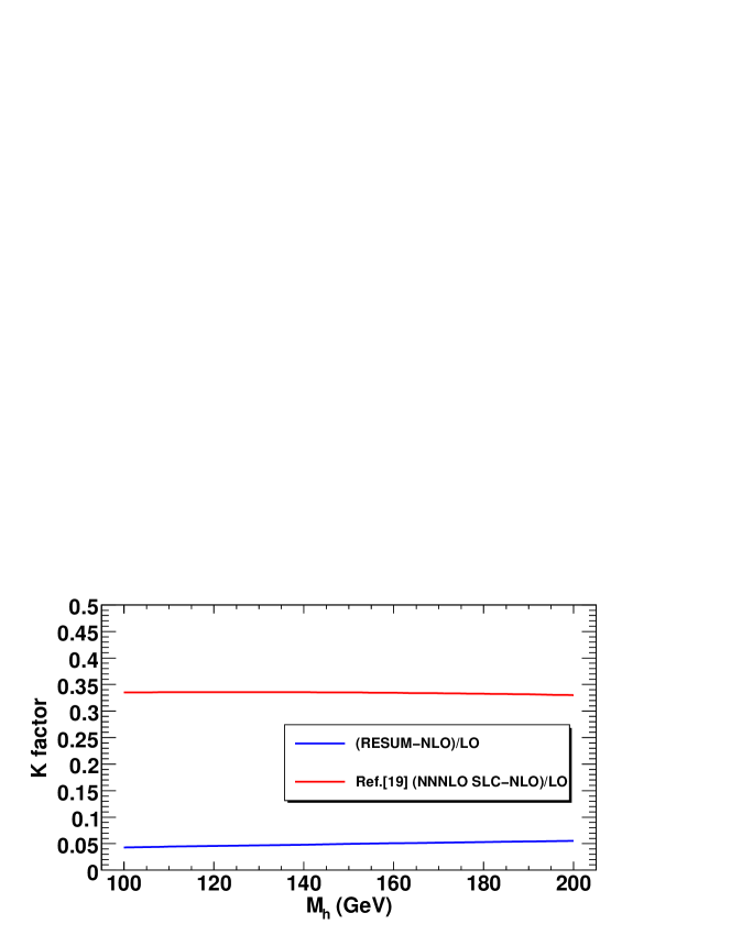
In Fig. 2 we show the K factor, which is defined as the ratios between the cross sections at the higher orders and the cross sections at the LO, for SM Higgs production cross sections with the NLL resummation effects and the NNNLO collinear and soft gluon effects in Ref. Kidonakis:2007ww , respectively, assuming $\mu_{r}=\mu_{f}=M_{h}$. We can see that our result is about $5$%, while their result shown in Ref. Kidonakis:2007ww is about $35$%.

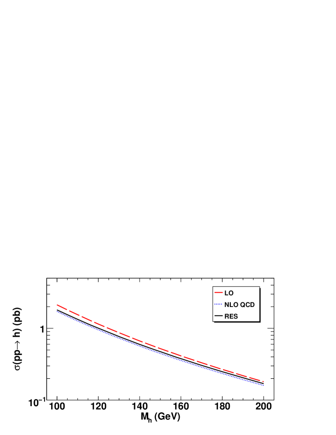
Fig. 3 shows the total cross sections for SM Higgs production as functions of the mass of Higgs boson including higher order QCD effects, assuming $\mu_{r}=\mu_{f}=M_{h}$. It can be seen from the figure that the total cross sections become small as the Higgs boson mass increases, which is due to the decreasing of the bottom quark density. The figure shows that the threshold resummation effects reduce the LO results significantly, and enhance the NLO results by a few percent generally.

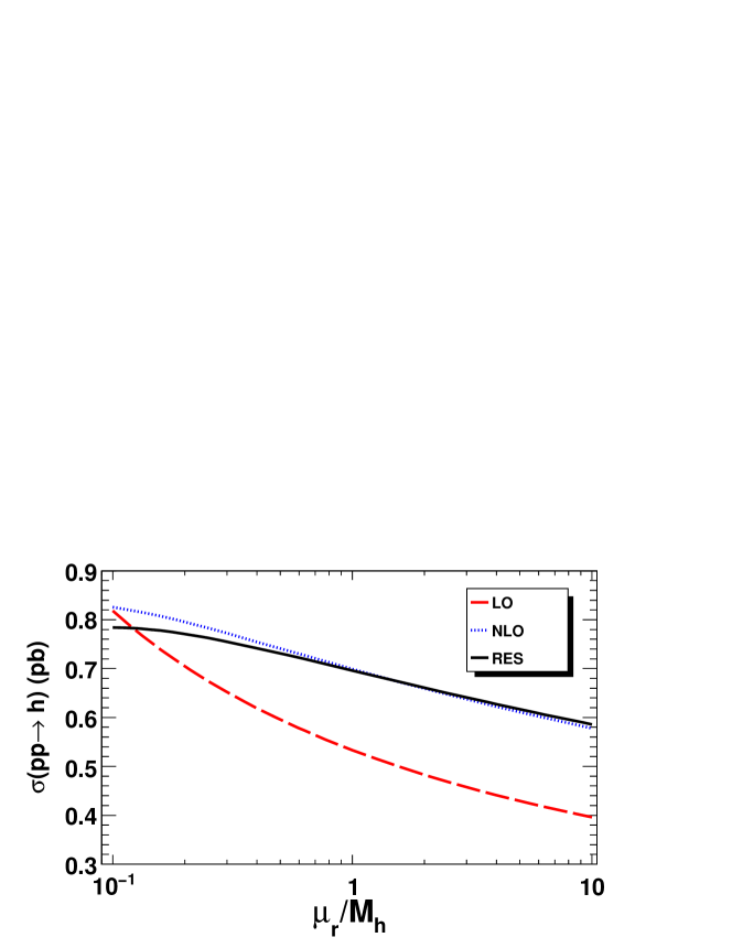
Fig. 4 shows the renormalization scale dependence of SM Higgs production, assuming $\mu_{f}=M_{h}/4$. We find that the renormalization scale dependence is reduced by the resummation effects, and the resummed cross section is very close to the NLO cross section in the vicinity of $\mu_{r}\sim M_{h}$. If restricting the renormalization scale to a factor of five above or below $M_{h}$, the scale dependence is reduced from about 50% at LO to 38% at NLO, and to about 30% at NLL.

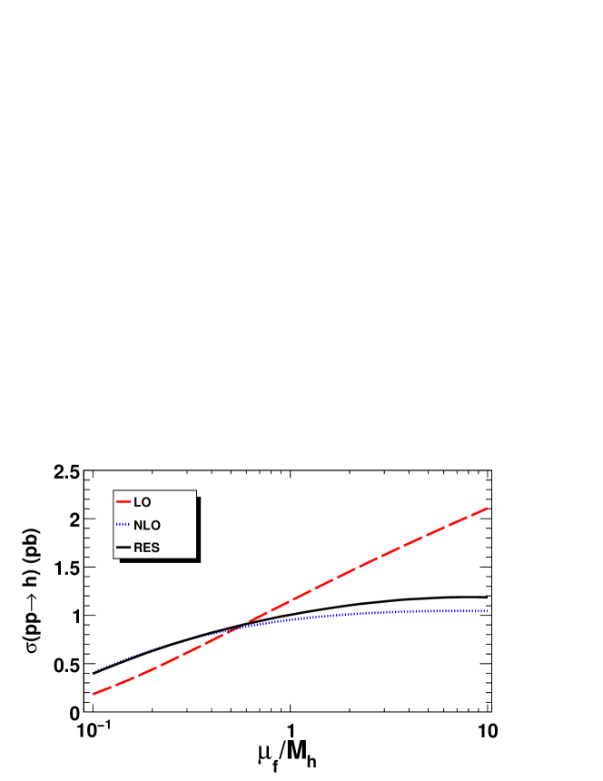
Fig. 5 gives the factorization scale dependence of SM Higgs production, assuming $\mu_{r}=M_{h}$. We see that the NLO corrections reduces the scale dependence significantly, and the resummation effects can not improve the scale dependence. This is due to the fact that the dominate contribution to the reduction of factorization scale dependence comes from the splitting processes of the initial states at the NLO, which are not included in the NLL resummation effects, while the NNLO corrections Harlander:2003ai can further reduce the factorization scale dependence. As shown in the figure, the resummation effects is small around $\mu_{f}\sim M_{h}/4$, which implies that the convergence of the resummed logarithmic terms is very well around such scale.

In Fig. 6 the resummation effects $\delta K$ are presented as a function of the SM Higgs boson mass $M_{h}$, assuming $\mu_{r}=M_{h}$ for $\mu_{f}=M_{h}/4$ and $\mu_{f}=M_{h}$, respectively. The results show that the resummation effects are quite small for $\mu_{f}=M_{h}/4$, about -1%, but for $\mu_{f}=M_{h}$, $\delta K$ can be over 5%. The resummation effects do not lead to large corrections relative to the NLO results, since the scaling variable $\tau=M^{2}_{h}/s$ is far away from 1 and the falling off of the bottom quark density is smooth.

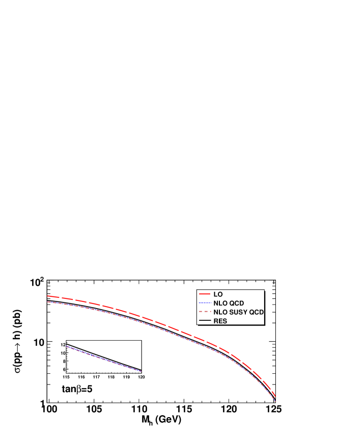
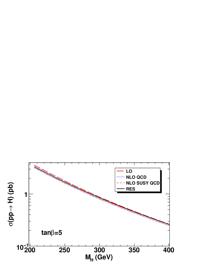
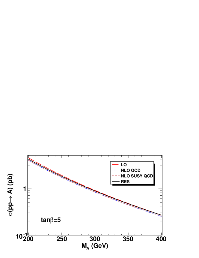
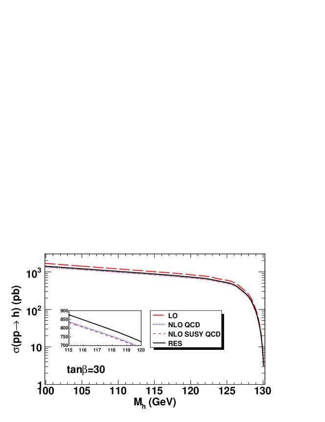
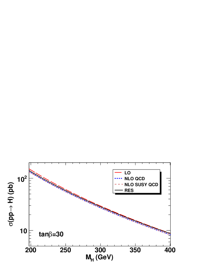
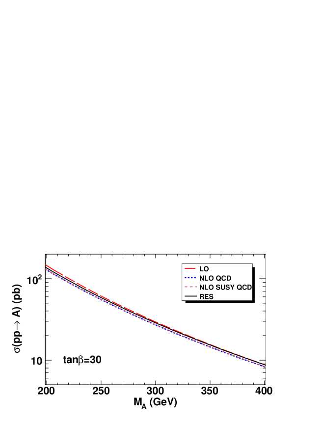
Figs. 7-12 show the total cross sections for $h$, $H$ and $A$ production as functions of their masses for the $m^{\rm max}_{h}$ scenario, assuming $\tan\beta=5$ and $30$, respectively. In these figures and the following, the variation on $M_{h}$ and $M_{H}$ is obtained from varying $M_{A}$. We find that in all cases, the NLO SUSY QCD corrections are negligible after employing the Improved Born Approximation, and the threshold resummation cross sections reduce the LO cross sections and enhance the NLO cross sections by a few percent.

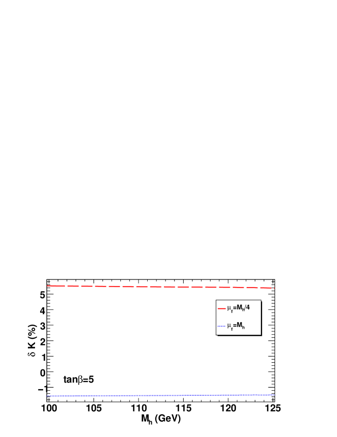
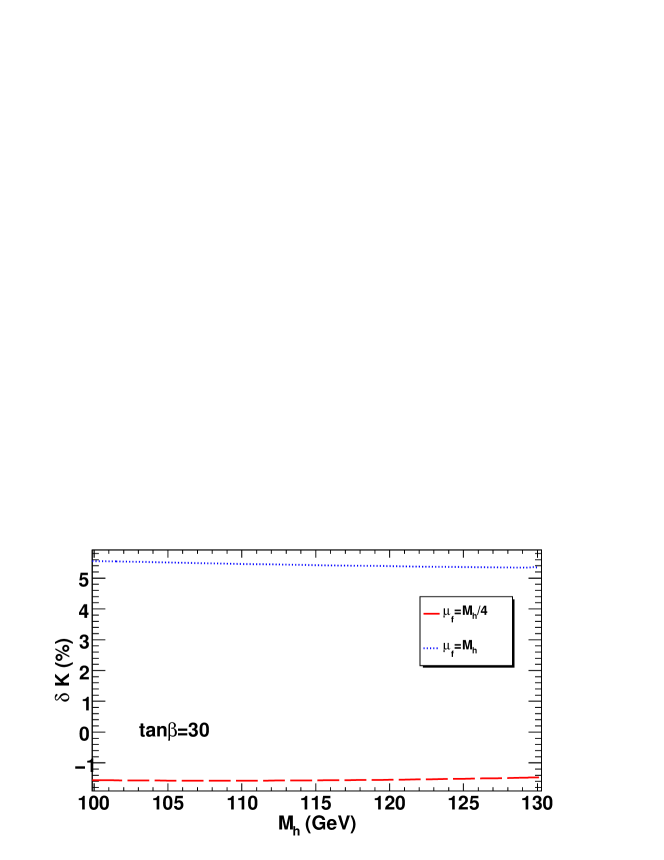
Figs. 13 and 14 present the resummation effects $\delta K$ as a function of $M_{h}$ assuming $\mu_{r}=M_{h}$ for $\tan\beta=5$ and $30$, respectively. In general, $\delta K$ is about -1% when $\mu_{f}=M_{h}/4$. However, the $\delta K$ can be larger than 5% when $\mu_{f}=M_{h}$. Note that the SUSY QCD corrections has little impact on the resummation effects $\delta K$ as shown in the figures, since the SUSY QCD do not give rise to new soft gluon interaction.

VI CONCLUSION

In conclusion, we have calculated the QCD effects in the production of the neutral Higgs boson via bottom quark fusion in both the SM and the MSSM at the LHC, which include not only the NLO QCD and SUSY QCD corrections, but also the NLL threshold resummation effects in the framework of SCET. Similar to Drell-Yan production Becher:2007ty ; drellyan , The resummation is achieved by separating the contribution from hard and soft scale into different matching coefficients and then summing the large logarithms of scale ratio via RG equation. This approach has the advantage that the ambiguity due to the Landau pole singularities is reduced. Our results of the NLO QCD and SUSY QCD corrections agree with the calculations reported in the previous literatures, and the resummatioin effects are about -1% and 5% for $\mu_{f}=M_{h}/4$ and $\mu_{f}=M_{h}$, respectively.

Appendix A

In this appendix, we collect the relevant MSSM Feynman rules as following higgshunter ; Kraml:1999qd :

1. The coupling between neutral Higgs boson and sbottom $H_{k}-\tilde{b}_{l}-{\tilde{b}_{m}}^{*}$:

$$i[R^{\tilde{b}}\hat{G}^{(k)}(R^{\tilde{b}})^{T}]_{lm}=i(G^{(k)})_{lm},$$

with

$$\hat{G}^{(h)} = \frac{g_{2}}{M_{W}}\left(\begin{array}[]{cc}M^{2}_{Z}\sin(\alpha+\beta)C_{bL}+m^{2}_{b}\frac{\sin\alpha}{\cos\beta}&\frac{m_{b}}{2}\left(A_{b}\frac{\sin\alpha}{\cos\beta}+\mu\frac{\cos\alpha}{\cos\beta}\right)\\ \frac{m_{b}}{2}\left(A_{b}\frac{\sin\alpha}{\cos\beta}+\mu\frac{\cos\alpha}{\cos\beta}\right)&-M^{2}_{Z}\sin(\alpha+\beta)C_{bR}+m^{2}_{b}\frac{\sin\alpha}{\cos\beta}\end{array}\right),$$

$$\hat{G}^{(H)}=\frac{g_{2}}{M_{W}}\left(\begin{array}[]{cc}-M^{2}_{Z}\cos(\alpha+\beta)C_{bL}-m^{2}_{b}\frac{\cos\alpha}{\cos\beta}&-\frac{m_{b}}{2}\left(A_{b}\frac{\cos\alpha}{\cos\beta}-\mu\frac{\sin\alpha}{\cos\beta}\right)\\ -\frac{m_{b}}{2}\left(A_{b}\frac{\cos\alpha}{\cos\beta}-\mu\frac{\sin\alpha}{\cos\beta}\right)&M^{2}_{Z}\cos(\alpha+\beta)C_{bR}-m^{2}_{b}\frac{\cos\alpha}{\cos\beta}\end{array}\right),$$

$$\hat{G}^{(A)}=i\frac{g_{2}m_{b}}{2m_{W}}\left(\begin{array}[]{cc}0&-A_{b}\tan\beta-\mu\\ A_{b}\tan\beta+\mu&0\end{array}\right).$$

2. The coupling between bottom, sbottom and gluino $b-\tilde{b}^{(*)}_{j}-\tilde{g}$:

Here $P_{L(R)}=(1\mp\gamma_{5})/2$ and $\mathbf{T}^{a}$ is the $SU(3)$ generator in fundamental representation.

Figure 2: The K factor of our results compared with those of Ref Kidonakis:2007ww , assuming $\mu_{r}=\mu_{f}=M_{h}$.

Figure 3: The total cross section for $pp\rightarrow h+X$ in SM at $\sqrt{s}=14$ TeV, assuming $\mu_{r}=\mu_{f}=M_{h}$.

Figure 4: The renormalization scale dependence of the total cross section for $pp\rightarrow h+X$ in SM at $\sqrt{s}=14$ TeV, assuming $\mu_{f}=M_{h}/4$ and $M_{h}=120$ GeV.

Figure 5: The factorization scale dependence of the total cross section for $pp\rightarrow h+X$ in SM at $\sqrt{s}=14$ TeV, assuming $\mu_{r}=M_{h}$ and $M_{h}=120$ GeV.

Figure 6: The NLL resummation effects with different factorization scale for $pp\rightarrow h+X$ in SM at $\sqrt{s}=14$ TeV, assuming $\mu_{r}=M_{h}$.

Figure 7: The MSSM total cross section for $pp\rightarrow h+X$ at $\sqrt{s}=14$ TeV in the $m^{\rm max}_{h}$ scenario, assuming $\mu_{r}=\mu_{f}=M_{h}$ and $\tan\beta=5$.

Figure 8: The total cross section for $pp\rightarrow H+X$ at $\sqrt{s}=14$ TeV in the $m^{\rm max}_{h}$ scenario, assuming $\mu_{r}=\mu_{f}=M_{H}$ and $\tan\beta=5$.

Figure 9: The total cross section for $pp\rightarrow A+X$ at $\sqrt{s}=14$ TeV in the $m^{\rm max}_{h}$ scenario, assuming $\mu_{r}=\mu_{f}=M_{A}$ and $\tan\beta=5$.

Figure 10: The total cross section for $pp\rightarrow h+X$ at $\sqrt{s}=14$ TeV in the $m^{\rm max}_{h}$ scenario, assuming $\mu_{r}=\mu_{f}=M_{h}$ and $\tan\beta=30$.

Figure 11: The total cross section for $pp\rightarrow H+X$ at $\sqrt{s}=14$ TeV in the $m^{\rm max}_{h}$ scenario, assuming $\mu_{r}=\mu_{f}=M_{H}$ and $\tan\beta=30$.

Figure 12: The total cross section for $pp\rightarrow A+X$ at $\sqrt{s}=14$ TeV in the $m^{\rm max}_{h}$ scenario, assuming $\mu_{r}=\mu_{f}=M_{A}$ and $\tan\beta=30$.

Figure 13: The comparison of NLL resummation effects at different factorization scale for $pp\rightarrow h+X$ at $\sqrt{s}=14$ TeV in the $m^{\rm max}_{h}$ scenario, assuming $\mu_{r}=M_{h}$ and $\tan\beta=5$.

Figure 14: The comparison of NLL resummation effects at different factorization scale for $pp\rightarrow h+X$ at $\sqrt{s}=14$ TeV in the $m^{\rm max}_{h}$ scenario, assuming $\mu_{r}=M_{h}$ and $\tan\beta=30$.

References

• (1) R. Barate et al. [LEP Working Group for Higgs boson searches and ALEPH Collaboration and and], Phys. Lett.  B 565, 61 (2003) [arXiv:hep-ex/0306033].
• (2) J. Alcaraz et al. [LEP Collaborations and ALEPH Collaboration and DELPHI Collaboration an], arXiv:0712.0929 [hep-ex].
• (3) H. E. Haber and R. Hempfling, Phys. Rev. Lett. 66 (1991) 1815; Y. Okada, M. Yamaguchi and T. Yanagida, Prog. Theor. Phys. 85 (1991) 1; J. Ellis, G. Ridolfi and F. Zwirner, Phys. Lett. B257 (1991) 83; S. Heinemeyer, hep-ph/0407244.
• (4) S. Dawson, C. B. Jackson, L. Reina and D. Wackeroth, Mod. Phys. Lett.  A 21, 89 (2006) [arXiv:hep-ph/0508293].
• (5) J. Campbell et al., arXiv:hep-ph/0405302.
• (6) D. Dicus, T. Stelzer, Z. Sullivan and S. Willenbrock, Phys. Rev.  D 59, 094016 (1999) [arXiv:hep-ph/9811492].
• (7) J. Campbell, R. K. Ellis, F. Maltoni and S. Willenbrock, Phys. Rev. D 67 (2003) 095002; S. Dawson, C. B. Jackson, L. Reina and D. Wackeroth, Phys. Rev. Lett. 94 (2005) 031802; S. Dawson and C. B. Jackson, Phys. Rev.  D 77, 015019 (2008) [arXiv:0709.4519 [hep-ph]].
• (8) R. Raitio and W. W. Wada, Phys. Rev. D 19 (1979) 941; S. Catani and L. Trentadue, Nucl. Phys.  B 327, 323 (1989); R. P. Kauffman, Phys. Rev.  D 44, 1415 (1991); C. Balázs, et al., Phys. Rev. D 59 (1999) 055016; E. Boos and T. Plehn, Phys. Rev. D 69 (2004) 094005; S. Dawson, C. B. Jackson, L. Reina and D. Wackeroth, Phys. Rev. D 69 (2004) 074027.
• (9) T. Plehn, Phys. Rev.  D 67, 014018 (2003) [arXiv:hep-ph/0206121]; S. Dittmaier, M. Kramer and M. Spira, Phys. Rev.  D 70, 074010 (2004) [arXiv:hep-ph/0309204]; S. Dawson, C. B. Jackson, L. Reina and D. Wackeroth, Mod. Phys. Lett.  A 21, 89 (2006) [arXiv:hep-ph/0508293]; C. Buttar et al.,[arXiv:hep-ph/0604120].
• (10) C. Balazs, H. J. He and C. P. Yuan, Phys. Rev.  D 60, 114001 (1999) [arXiv:hep-ph/9812263].
• (11) F. Maltoni, Z. Sullivan and S. Willenbrock, Phys. Rev.  D 67, 093005 (2003) [arXiv:hep-ph/0301033].
• (12) R. V. Harlander and W. B. Kilgore, Phys. Rev.  D 68, 013001 (2003) [arXiv:hep-ph/0304035].
• (13) S. Dittmaier, M. Kramer, A. Muck and T. Schluter, JHEP 0703, 114 (2007) [arXiv:hep-ph/0611353].
• (14) G. Sterman, Nucl. Phys.  B 281, 310 (1987); N. Kidonakis and G. Sterman, Phys. Lett.  B 387, 867 (1996); N. Kidonakis and G. Sterman, Nucl. Phys.  B 505, 321 (1997) [arXiv:hep-ph/9705234].
• (15) S. Catani and L. Trentadue, Nucl. Phys.  B 327, 323 (1989).
• (16) B. Field, arXiv:hep-ph/0407254.
• (17) A. Belyaev, P. M. Nadolsky and C. P. Yuan, JHEP 0604, 004 (2006) [arXiv:hep-ph/0509100].
• (18) V. Ravindran, Nucl. Phys.  B 752, 173 (2006) [arXiv:hep-ph/0603041].
• (19) N. Kidonakis, Phys. Rev.  D 77, 053008 (2008) [arXiv:0711.0142 [hep-ph]].
• (20) C. W. Bauer, S. Fleming and M. E. Luke, Phys. Rev. D 63, 014006 (2001); C. W. Bauer, S. Fleming, D. Pirjol and I. W. Stewart, Phys. Rev. D 63, 114020 (2001); C. W. Bauer and I. W. Stewart, Phys. Lett. B 516, 134 (2001).
• (21) A. Sirlin, Phys. Rev. D 22 (1980) 971; W. J. Marciano and A. Sirlin, Phys. Rev. D 22 (1980) 2695; Phys. Rev. D 31 (1985) 213 (E); A. Sirlin and W. J. Marciano, Nucl. Phys. B 189 (1981) 442; K. I. Aoki et al., Prog. Theor. Phys. Suppl. 73 (1982) 1.
• (22) E. Braaten and J. P. Leveille, Phys. Rev.  D 22, 715 (1980).
• (23) A. Denner, Fortschr. Phys. 41 (1993) 4.
• (24) F. Bloch and A. Nordsieck, Phys. Rev.  52, 54 (1937).
• (25) G. Altarelli, R. K. Ellis, G. Martinelli, Nucl. Phys. B 157 (1979) 461; J. C. Collins, D. E. Soper and G. Sterman, in: Perturbative Quantum Chromodynamics, ed. A.H. Mueller (World Scientific, 1989).
• (26) G. Altarelli and G. Parisi, Nucl. Phys.  B 126, 298 (1977).
• (27) A. Dabelstein, Nucl. Phys.  B 456, 25 (1995) [arXiv:hep-ph/9503443].
• (28) A. V. Manohar, Phys. Rev. D 68, 114019 (2003).
• (29) T. Becher, M. Neubert and B. D. Pecjak, JHEP 0701, 076 (2007); T. Becher and M. Neubert, Phys. Rev. Lett.  97, 082001 (2006).
• (30) T. Becher, M. Neubert and G. Xu, JHEP 0807, 030 (2008) [arXiv:0710.0680 [hep-ph]].
• (31) A. Idilbi and X. d. Ji, Phys. Rev.  D 72, 054016 (2005); A. Idilbi, X. d. Ji and F. Yuan, Nucl. Phys.  B 753, 42 (2006).
• (32) Y. Gao, C. S. Li and J. J. Liu, Phys. Rev.  D 72, 114020 (2005); A. Idilbi, X. d. Ji, J. P. Ma and F. Yuan, Phys. Rev.  D 73, 077501 (2006); V. Ahrens, T. Becher, M. Neubert and L. L. Yang, Phys. Rev.  D 79, 033013 (2009) arXiv:0808.3008 [hep-ph]; V. Ahrens, T. Becher, M. Neubert and L. L. Yang, arXiv:0809.4283 [hep-ph].
• (33) M. D. Schwartz, Phys. Rev.  D 77, 014026 (2008).
• (34) L. L. Yang, C. S. Li, Y. Gao and J. J. Liu, Phys. Rev.  D 73, 074017 (2006); A. Idilbi, C. Kim and T. Mehen, arXiv:0903.3668 [hep-ph].
• (35) J. C. Collins, D. E. Soper and G. Sterman, Adv. Ser. Direct. High Energy Phys.  5, 1 (1988) [arXiv:hep-ph/0409313].
• (36) C. W. Bauer, S. Fleming, D. Pirjol, I. Z. Rothstein and I. W. Stewart, Phys. Rev.  D 66, 014017 (2002) [arXiv:hep-ph/0202088].
• (37) G. P. Korchemsky and A. V. Radyushkin, Nucl. Phys.  B 283, 342 (1987).
• (38) I. A. Korchemskaya and G. P. Korchemsky, Phys. Lett.  B 287, 169 (1992).
• (39) G. P. Korchemsky and G. Marchesini, Phys. Lett.  B 313, 433 (1993).
• (40) A. V. Belitsky, Phys. Lett.  B 442, 307 (1998) [arXiv:hep-ph/9808389].
• (41) C. S. Li, Z. Li and C. P. Yuan, arXiv:0903.1798 [hep-ph].
• (42) G. P. Korchemsky and S. Tafat, JHEP 0010, 010 (2000) [arXiv:hep-ph/0007005]; A. H. Hoang and I. W. Stewart, Phys. Lett.  B 660, 483 (2008) [arXiv:0709.3519 [hep-ph]].
• (43) G. Curci, W. Furmanski and R. Petronzio, Nucl. Phys. B 175, 27 (1980); W. Furmanski and R. Petronzio, Phys. Lett. B 97, 437 (1980).
• (44) O. V. Tarasov, A. A. Vladimirov and A. Y. Zharkov, Phys. Lett.  B 93, 429 (1980); S. A. Larin and J. A. M. Vermaseren, Phys. Lett.  B 303, 334 (1993) [arXiv:hep-ph/9302208].
• (45) S. Catani, M. L. Mangano, P. Nason and L. Trentadue, Nucl. Phys.  B 478, 273 (1996) [arXiv:hep-ph/9604351].
• (46) A. Kulesza, G. Sterman and W. Vogelsang, Phys. Rev. D 66, 014011 (2002).
• (47) C. Amsler et al. [Particle Data Group], Phys. Lett.  B 667, 1 (2008).
• (48) S. G. Gorishny, A. L. Kataev, S. A. Larin and L. R. Surguladze, Mod. Phys. Lett. A 5 (1990) 2703; Phys. Rev. D 43 (1991) 1633; A. Djouadi, M. Spira and P. M. Zerwas, Z. Phys. C 70 (1996) 427; A. Djouadi, J. Kalinowski, M. Spira, Comput. Phys. Commun. 108 (1998) 56; M. Spira, Fortschr. Phys. 46 (1998) 203.
• (49) P. M. Nadolsky et al., Phys. Rev.  D 78, 013004 (2008) [arXiv:0802.0007 [hep-ph]].
• (50) M. Carena, D. Garcia, U. Nierste, C. E. M. Wagner, Nucl. Phys. B 577 (2000) 88. [arXiv:hep-ph/9912516].
• (51) J. Guasch, P. Hafliger and M. Spira, Phys. Rev.  D 68, 115001 (2003) [arXiv:hep-ph/0305101].
• (52) S. Heinemeyer, W. Hollik and G. Weiglein, Comput. Phys. Commun.  124, 76 (2000) [arXiv:hep-ph/9812320].
• (53) M. S. Carena, S. Heinemeyer, C. E. M. Wagner and G. Weiglein, Eur. Phys. J.  C 26, 601 (2003) [arXiv:hep-ph/0202167].
• (54) S. Heinemeyer, W. Hollik and G. Weiglein, JHEP 0006, 009 (2000) [arXiv:hep-ph/9909540].
• (55) J. F. Gunion, H. E. Haber, G. Kane and S. Dawson, The Higgs Hunter’s Guide (ADDison–Wesley, Redwood City, CA, 1990).
• (56) S. Kraml, arXiv:hep-ph/9903257.
Refer to caption