Theory of incompressible MHD turbulence with scale-dependent alignment and cross-helicity

Abstract

A phenomenological anisotropic theory of MHD turbulence with nonvanishing cross-helicity is constructed based on Boldyrev’s phenomenology and probabilities $p$ and $q$ for fluctuations $\delta\bm{v}_{\perp}$ and $\delta\bm{b}_{\perp}$ to be positively or negatively aligned. The positively aligned fluctuations occupy a fractional volume $p$ and the negatively aligned fluctuations occupy a fractional volume $q$. Guided by observations suggesting that the normalized cross-helicity $\sigma_{c}$ and the probabilities $p$ and $q$ are approximately scale invariant in the inertial range, a generalization of Boldyrev’s theory is derived that depends on the three ratios $w^{+}/w^{-}$, $\epsilon^{+}/\epsilon^{-}$, and $p/q$. It is assumed that the cascade process for positively and negatively aligned fluctuations are both in a state of critical balance and that the eddy geometries are scale invariant. The theory reduces to Boldyrev’s original theory when $\sigma_{c}=0$, $\epsilon^{+}=\epsilon^{-}$, and $p=q$ and extends the theory of Perez and Boldyrev when $\sigma_{c}\neq 0$. The theory is also an anisotropic generalization of the theory of Dobrowolny, Mangeney, and Veltri.

I Introduction

Phenomenological theories of incompressible MHD turbulence that take into account the anisotropy of the fluctuations with respect to the direction of the mean magnetic field $\bm{B}_{0}$ were pioneered by Goldreich & Sridhar and others in the 1990s. The influencial and somewhat controversial theory of Goldreich & Sridhar (Goldreich and Sridhar, 1995, 1997) established the idea that the timescale or coherence time for motions of a turbulent eddy parallel and perpendicular to $\bm{B}_{0}$ must be equal to each other and this unique timescale then defines the energy cascade time. This concept, called critical balance, leads immediately to the perpendicular energy spectrum $E(k_{\perp})\propto k_{\perp}^{-5/3}$ and to the scaling relation $k_{\parallel}\propto k_{\perp}^{2/3}$ describing the anisotropy of the turbulent eddies.

The decade following the publication of the paper by Goldreich & Sridhar in 1995 was a time when significant advances in computing power were brought to bear on computational studies of MHD turbulence. Simulations of incompressible MHD turbulence during this time showed that when the mean magnetic field is strong, $B_{0}^{2}\gg(\delta b)^{2}$, the perpendicular energy spectrum exhibits a power-law scaling closer to $k_{\perp}^{-3/2}$ than $k_{\perp}^{-5/3}$ (Maron and Goldreich, 2001; Müller et al., 2003; Müller and Grappin, 2005). Motivated by this result, Boldyrev modified the Goldreich & Sridhar theory to explain the $k_{\perp}^{-3/2}$ power-law seen in simulations (Boldyrev, 2005, 2006). A new concept that emerged in Boldyrev’s theory is the scale dependent alignment of velocity and magnetic field fluctuations whereby the angle $\theta$ formed by $\delta\bm{v}_{\perp}$ and $\delta\bm{b}_{\perp}$ scales like $\lambda_{\perp}^{1/4}$ in the inertial range. This alignment effect weakens the nonlinear interactions and yields the perpendicular energy spectrum $E(k_{\perp})\propto k_{\perp}^{-3/2}$. Evidence for this alignment effect has been found in numerical simulations of incompressible MHD turbulence (Mason et al., 2006, 2008) and in studies of solar wind data (Podesta et al., 2008, 2009).

The phenomenological theory of Galtier et al. (2005) can also be used to explain the observed $k_{\perp}^{-3/2}$ energy spectrum. Using a slightly modified critical balance relation that retains the $k_{\parallel}\propto k_{\perp}^{2/3}$ scaling of the Goldreich & Sridhar theory, their model admits the $k_{\perp}^{-3/2}$ energy spectrum (as well as other solutions). However, the theory of Galtier et al. (2005) does not include the scale dependent alignment that arises in Boldyrev’s theory and, more importantly, is seen in the solar wind (Podesta et al., 2008, 2009).

The theories discussed so far (Goldreich and Sridhar, 1995, 1997; Boldyrev, 2005, 2006; Galtier et al., 2005) all assume that the cross-helicity vanishes and, therefore, these theories cannot be applied to solar wind turbulence. When the cross-helicity of the turbulence is nonzero it is necessary to take into account the cascades of both energy and cross-helicity. A generalization of the Goldreich & Sridhar theory to turbulence with nonvanishing cross-helicity, also called imbalanced turbulence, has been developed by Lithwick, Goldreich, & Sridhar (Lithwick et al., 2007). Other theories of imbalanced turbulence have been derived by Beresnyak & Lazarian (Beresnyak and Lazarian, 2008) and Chandran (Chandran, 2008; Chandran et al., 2009). However, none of these theories contains the scale dependent alignment of velocity and magnetic field fluctuations seen in the solar wind. Therefore, to develop a theory that may be applicable to solar wind turbulence it is of interest to generalize Boldyrev’s theory to incompressible MHD turbulence with non-vanishing cross-helicity. An extension of Boldyrev’s theory to imbalanced turbulence has been discussed by Perez & Boldyrev (Perez and Boldyrev, 2009). The purpose of the present paper is to develop a theoretical framework which generalizes the results of Perez & Boldyrev and is consistent with solar wind observations.

Our theory is founded, in part, on two new solar wind observations presented in this paper. The first is the observation that the normalized cross-helicity $\sigma_{c}$, the ratio of cross-helicity to energy, is scale invariant in the inertial range. The second is the observation that the probabilities $p$ and $q$ that fluctuations are positively or negatively aligned, respectively, are also scale invariant, that is, these quantities are approximately constant in the inertial range. Experimental evidence for the scale invariance of $\sigma_{c}$ comes from solar wind observations by Marsch and Tu (1990) and also Figure 1 below, and from numerical simulations (Verma et al., 1996; Perez and Boldyrev, 2009). Evidence for the scale invariance of $p$ and $q$ is shown in Figure 2 below. Assuming these quantities are all scale invariant we deduce expressions for the energy cascade rates and the rms fluctuations that generalize the results in (Boldyrev, 2006) and (Perez and Boldyrev, 2009) and are consistent with the concept of scale dependent alignment of velocity and magnetic field fluctuations, a concept neglected in other phenomenological theories (Galtier et al., 2005; Lithwick et al., 2007; Beresnyak and Lazarian, 2008; Chandran, 2008). The resulting theory, which is founded on the concept of scale-invariance and grounded in solar wind observations, contains the theories of Boldyrev (2006) and Perez and Boldyrev (2009) as special cases, but opens up a broader range of physical possibilities.

Consistent with numerical simulations and solar wind observations, in our approach the fluctuations at a given point may assume one of two possible states referred to as positively aligned $\delta\bm{v}_{\perp}\cdot\delta\bm{b}_{\perp}>0$ and negatively aligned $\delta\bm{v}_{\perp}\cdot\delta\bm{b}_{\perp}<0$. Each state is characterized by its own rms energy $v^{2}$, alignment angle $\theta$, and nonlinear timescale $\tau$. Positively aligned fluctuations have a characteristic spatial gradient which determines their nonlinear timescale and negatively aligned fluctuations have a different spatial gradient which determines their nonlinear timescale. These timescales are estimated from the nonlinear terms in the MHD equations as described in sections 2 and 3.

Section 2 describes the geometries of velocity and magnetic field fluctuations that are either aligned ‘$\uparrow$’ or anti-aligned ‘$\downarrow$’ and these are used to form estimates of the nonlinear terms in the MHD equations. From this foundation, estimates of the energy cascade times are constructed in section 3 and the theory of the energy cascade process is developed in section 4. The summary and conclusions are presented in section 5.

II Fluctuations in imbalanced turbulence

Consider velocity and magnetic field fluctuations measured between two points separated by a distance $\lambda_{\perp}$ in the field perpendicular plane. Let $\bm{v}$ and $\bm{b}$ denote the fluctuations in the plane perpendicular to the local mean magnetic field, where $\bm{v}$ and $\bm{b}$ are both measured in velocity units. Suppose that $\bm{v}$ and $\bm{b}$ are aligned with some small angle $\theta>0$ and assume, as for Alfvén waves, that $|\bm{v}|=|\bm{b}|$. Then $\bm{w}^{+}=\bm{v}+\bm{b}$ is nearly aligned with $\bm{v}$ and $\bm{w}^{-}=\bm{v}-\bm{b}$ is nearly perpendicular to $\bm{v}$ as sketched in Figure 1.

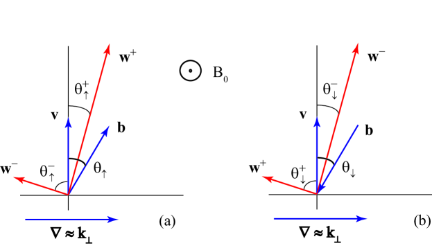
Figure 1: Geometry of the fluctuation vectors $\bm{v}$ and $\bm{b}$ for positively aligned fluctuations (a) denoted by ‘$\uparrow$’ and negatively aligned fluctuations (b) denoted by ‘$\downarrow$’. The gradient is perpendicular to the velocity fluctuation $\bm{v}$. The magnitude of $\bm{v}$ for positively and negatively aligned fluctuations are $v_{\uparrow}$ and $v_{\downarrow}$, respectively. The angles formed by $\bm{v}$ and $\bm{b}$, $\theta_{\uparrow}$ and $\theta_{\downarrow}$, are both assumed to be small.

It follows from the identity $\bm{w}^{\pm}\times\bm{v}=\mp\bm{v}\times\bm{b}$ that

$$w^{+}\sin\theta^{+}=v\sin\theta=w^{-}\sin\theta^{-},$$ (1)

where $\theta^{+}$ is the angle formed by $\bm{w}^{+}$ and $\bm{v}$, $\theta^{-}$ is the angle formed by $\bm{w}^{-}$ and $\bm{v}$, and $\theta$ is the angle formed by $\bm{v}$ and $\bm{b}$. In addition, $\theta^{+}+\theta^{-}=\pi/2$. Following Boldyrev (2006), suppose that the gradient of the fluctuations is in the direction perpendicular to $\bm{v}$. In this case,

$$(\bm{w}^{-}\cdot\nabla)\simeq\frac{w^{-}\sin\theta^{-}}{\lambda_{\perp}}=\frac{v\sin\theta}{\lambda_{\perp}}$$ (2)

and

$$(\bm{w}^{+}\cdot\nabla)\simeq\frac{w^{+}\sin\theta^{+}}{\lambda_{\perp}}=\frac{v\sin\theta}{\lambda_{\perp}}.$$ (3)

The time rate of change caused by nonlinear interactions is estimated from the relations

$$\frac{\partial}{\partial t}\frac{|\bm{w}^{+}|^{2}}{2}\simeq\bm{w}^{+}\cdot(\bm{w}^{-}\cdot\nabla)\bm{w}^{+}$$ (4)

and

$$\frac{\partial}{\partial t}\frac{|\bm{w}^{-}|^{2}}{2}\simeq\bm{w}^{-}\cdot(\bm{w}^{+}\cdot\nabla)\bm{w}^{-}.$$ (5)

If $\bm{v}$ and $\bm{b}$ are aligned with some small angle $\theta$, then the fluctuations are called “positively aligned” and denoted by ‘$\uparrow$’ (Figure 1a). Similarly, if $\bm{v}$ and $-\bm{b}$ are aligned with some small angle $\theta$, then the fluctuations are called “negatively aligned” or “anti-aligned” and denoted by ‘$\downarrow$’ (Figure 1b). For positively aligned fluctuations, equations (2)–(5) imply

$$\frac{\partial}{\partial t}\frac{(w^{+}_{\uparrow})^{2}}{2}\simeq\frac{(w^{+}_{\uparrow})^{2}w^{-}_{\uparrow}\sin\theta^{-}_{\uparrow}}{\lambda_{\perp}}=\frac{(w^{+}_{\uparrow})^{2}v_{\uparrow}\sin\theta_{\uparrow}}{\lambda_{\perp}}$$ (6)

and

$$\frac{\partial}{\partial t}\frac{(w^{-}_{\uparrow})^{2}}{2}\simeq\frac{(w^{-}_{\uparrow})^{2}w^{+}_{\uparrow}\sin\theta^{+}_{\uparrow}}{\lambda_{\perp}}=\frac{(w^{-}_{\uparrow})^{2}v_{\uparrow}\sin\theta_{\uparrow}}{\lambda_{\perp}},$$ (7)

where $\theta_{\uparrow}$ is the angle formed by $\bm{v}$ and $\bm{b}$ and quantities with the subscript $\uparrow$ describe positively aligned fluctuations. It is clear from the middle term in equation (6) that the time rate of change of $w^{+}_{\uparrow}$ depends on $w^{-}_{\uparrow}$, consistent with the nonlinear terms in the MHD equations, although this dependence is not immediately apparent in the last term in (6). For negatively aligned fluctuations, equations (2)–(5) imply

$$\frac{\partial}{\partial t}\frac{(w^{+}_{\downarrow})^{2}}{2}\simeq\frac{(w^{+}_{\downarrow})^{2}w^{-}_{\downarrow}\sin\theta^{-}_{\downarrow}}{\lambda_{\perp}}=\frac{(w^{+}_{\downarrow})^{2}v_{\downarrow}\sin\theta_{\downarrow}}{\lambda_{\perp}}$$ (8)

and

$$\frac{\partial}{\partial t}\frac{(w^{-}_{\downarrow})^{2}}{2}\simeq\frac{(w^{-}_{\downarrow})^{2}w^{+}_{\downarrow}\sin\theta^{+}_{\downarrow}}{\lambda_{\perp}}=\frac{(w^{-}_{\downarrow})^{2}v_{\downarrow}\sin\theta_{\downarrow}}{\lambda_{\perp}},$$ (9)

where $\theta_{\downarrow}$ is the angle formed by $\bm{v}$ and $-\bm{b}$ and quantities with the subscript $\downarrow$ describe negatively aligned fluctuations. Here, $0<\theta_{\uparrow}<\pi/2$ and $0<\theta_{\downarrow}<\pi/2$.

In general, the fluctuations $\bm{v}$ and $\bm{b}$ observed at any point $(\bm{x},t)$ are either positively or negatively aligned. For a point $(\bm{x},t)$ picked at random, let $p$ and $q$ be the probabilities the alignment is positive or negative, respectively ($p+q=1$). Then, on average,

$$\frac{\partial}{\partial t}\frac{(\tilde{w}^{+})^{2}}{2}\simeq\frac{1}{\lambda_{\perp}}\big{[}p(w^{+}_{\uparrow})^{2}v_{\uparrow}\sin\theta_{\uparrow}+q(w^{+}_{\downarrow})^{2}v_{\downarrow}\sin\theta_{\downarrow}\big{]}$$ (10)

and

$$\frac{\partial}{\partial t}\frac{(\tilde{w}^{-})^{2}}{2}\simeq\frac{1}{\lambda_{\perp}}\big{[}p(w^{-}_{\uparrow})^{2}v_{\uparrow}\sin\theta_{\uparrow}+q(w^{-}_{\downarrow})^{2}v_{\downarrow}\sin\theta_{\downarrow}\big{]},$$ (11)

where the rms values $\tilde{w}^{\pm}$ are defined by

$$(\tilde{w}^{+})^{2} =p(w_{\uparrow}^{+})^{2}+q(w_{\downarrow}^{+})^{2},$$ (12)

$$(\tilde{w}^{-})^{2} =p(w_{\uparrow}^{-})^{2}+q(w_{\downarrow}^{-})^{2}.$$ (13)

The following relations also hold. For a positively aligned fluctuation, assuming $|\bm{v}|=|\bm{b}|$,

$$\bm{w}_{\uparrow}^{+}\cdot\bm{w}_{\uparrow}^{+} =2v_{\uparrow}^{2}(1+\cos\theta_{\uparrow}),$$ (14)

$$\bm{w}_{\uparrow}^{-}\cdot\bm{w}_{\uparrow}^{-} =2v_{\uparrow}^{2}(1-\cos\theta_{\uparrow}),$$ (15)

and $w^{+}_{\uparrow}w^{-}_{\uparrow}=2v_{\uparrow}^{2}\sin\theta_{\uparrow}$. The energy of a positively aligned fluctuation is $v_{\uparrow}^{2}$. For a negatively aligned fluctuation

$$\bm{w}_{\downarrow}^{+}\cdot\bm{w}_{\downarrow}^{+} =2v_{\downarrow}^{2}(1-\cos\theta_{\downarrow}),$$ (16)

$$\bm{w}_{\downarrow}^{-}\cdot\bm{w}_{\downarrow}^{-} =2v_{\downarrow}^{2}(1+\cos\theta_{\downarrow}),$$ (17)

and $w^{+}_{\downarrow}w^{-}_{\downarrow}=2v_{\downarrow}^{2}\sin\theta_{\downarrow}$. The energy of a negatively aligned fluctuation is $v_{\downarrow}^{2}$. Thus, the rms values (12) and (13) are

$$(\tilde{w}^{+})^{2} =2\big{[}pv_{\uparrow}^{2}(1+\cos\theta_{\uparrow})+qv_{\downarrow}^{2}(1-\cos\theta_{\downarrow})\big{]},$$ (18)

$$(\tilde{w}^{-})^{2} =2\big{[}pv_{\uparrow}^{2}(1-\cos\theta_{\uparrow})+qv_{\downarrow}^{2}(1+\cos\theta_{\downarrow})\big{]}.$$ (19)

If the angles are small, $\theta_{\uparrow}\ll 1$ and $\theta_{\downarrow}\ll 1$, then the small parameter $\theta$ can be used to order the terms in equations (18) and (19) so that to leading order

$$(\tilde{w}^{+})^{2}\simeq 4v_{\uparrow}^{2}p\qquad\mbox{and}\qquad(\tilde{w}^{-})^{2}\simeq 4v_{\downarrow}^{2}q,$$ (20)

where $p+q=1$. This may be derived as follows. In equations (18) and (19) assume that the angles are both small and then substitute $1+\cos\theta\simeq 2$ and $1-\cos\theta=2\sin^{2}(\theta/2)$ to obtain

$$(\tilde{w}^{+})^{2}\simeq 4\big{[}pv_{\uparrow}^{2}+qv_{\downarrow}^{2}\sin^{2}(\theta_{\downarrow}/2)\big{]}\\$$ (21)

and

$$(\tilde{w}^{-})^{2}\simeq 4\big{[}pv_{\uparrow}^{2}\sin^{2}(\theta_{\uparrow}/2)+qv_{\downarrow}^{2}\big{]}.$$ (22)

As $\lambda_{\perp}\rightarrow 0$, both $\theta_{\uparrow}\rightarrow 0$ and $\theta_{\downarrow}\rightarrow 0$ and, therefore, to first order, the terms proportional to $\sin^{2}(\theta)$ may be neglected. Alternatively, note that

$$\bigg{(}\frac{\tilde{w}^{+}}{\tilde{w}^{-}}\bigg{)}^{2}\simeq\frac{(pv_{\uparrow}^{2}/qv_{\downarrow}^{2})+\sin^{2}(\theta_{\downarrow}/2)}{(pv_{\uparrow}^{2}/qv_{\downarrow}^{2})\sin^{2}(\theta_{\uparrow}/2)+1}.$$ (23)

As discussed below, solar wind observations show that this quantity is approximately constant in the inertial range. Now, as $\theta_{\uparrow}\rightarrow 0$ and $\theta_{\downarrow}\rightarrow 0$ the only way that this can remain constant is if $pv_{\uparrow}^{2}/qv_{\downarrow}^{2}$ is bounded away from zero and

$$\bigg{(}\frac{\tilde{w}^{+}}{\tilde{w}^{-}}\bigg{)}^{2}\simeq\frac{pv_{\uparrow}^{2}}{qv_{\downarrow}^{2}}.$$ (24)

This justifies the approximation in Eqn (20).

Equation (20) shows that at a given scale $\lambda_{\perp}$ the total energy $[(\tilde{w}^{+})^{2}+(\tilde{w}^{-})^{2}]/4$ is partitioned into two parts, the energy $(\tilde{w}^{+})^{2}/4$ associated with positive alignment and the energy $(\tilde{w}^{-})^{2}/4$ associated with negative alignment. The normalized cross-helicity $\sigma_{c}$ is defined as the ratio of the cross-helicity to the energy at a given scale and can be written

$$\sigma_{c}=\frac{(\tilde{w}^{+})^{2}-(\tilde{w}^{-})^{2}}{(\tilde{w}^{+})^{2}+(\tilde{w}^{-})^{2}}.$$ (25)

For small angles, equations (10) and (11) become, to leading order,

$$\frac{\partial}{\partial t}\frac{(\tilde{w}^{+})^{2}}{2} \simeq\frac{4pv_{\uparrow}^{3}\theta_{\uparrow}}{\lambda_{\perp}},$$ (26)

$$\frac{\partial}{\partial t}\frac{(\tilde{w}^{-})^{2}}{2} \simeq\frac{4qv_{\downarrow}^{3}\theta_{\downarrow}}{\lambda_{\perp}}.$$ (27)

To express these in terms of the rms values $\tilde{w}^{\pm}$, eliminate $v_{\uparrow}$ and $v_{\downarrow}$ using equation (20). This yields

$$\frac{\partial}{\partial t}\frac{(\tilde{w}^{+})^{2}}{2} \simeq\frac{(\tilde{w}^{+})^{3}\theta_{\uparrow}}{2\lambda_{\perp}p^{1/2}},$$ (28)

$$\frac{\partial}{\partial t}\frac{(\tilde{w}^{-})^{2}}{2} \simeq\frac{(\tilde{w}^{-})^{3}\theta_{\downarrow}}{2\lambda_{\perp}q^{1/2}}.$$ (29)

These estimates shall be used to derive the cascade times.

III Energy cascade time

When nonlinear interactions are strong and a large number of Fourier modes are excited, fluctuations occur continuously in time and space. During a time $\tau$ the fractional change in the quantity $(\tilde{w}^{+})^{2}$ is, from (28),

$$\chi^{+}(\tau)\simeq\frac{(w^{+})^{3}\theta_{\uparrow}}{2\lambda_{\perp}p^{1/2}}\cdot\frac{2\tau}{(w^{+})^{2}}=\frac{w^{+}\theta_{\uparrow}\tau}{\lambda_{\perp}p^{1/2}},\qquad\tau\leq\tau^{+},$$ (30)

where $\tau^{+}$ is the cascade time at the lengthscale $\lambda_{\perp}$ and the tildes have been dropped. Similarly, the fractional change in the quantity $(\tilde{w}^{-})^{2}$ is, from (29),

$$\chi^{-}(\tau)\simeq\frac{(w^{-})^{3}\theta_{\downarrow}}{2\lambda_{\perp}q^{1/2}}\cdot\frac{2\tau}{(w^{-})^{2}}=\frac{w^{-}\theta_{\downarrow}\tau}{\lambda_{\perp}q^{1/2}},\qquad\tau\leq\tau^{-},$$ (31)

where $\tau^{-}$ is the cascade time of $\tilde{w}^{-}$ and the tildes have been dropped for brevity. Hereafter, the tildes will be omitted and $w^{+}$ and $w^{-}$ will always represent the rms values.

According to the definition of the energy cascade time, the fractional change $\chi^{+}$ is of order unity when the interaction time $\tau$ is equal to the cascade time $\tau^{+}$. Therefore, the relations (30) and (31) imply

$$\tau^{+}\simeq\frac{\lambda_{\perp}p^{1/2}}{w^{+}\theta_{\uparrow}},\qquad\tau^{-}\simeq\frac{\lambda_{\perp}q^{1/2}}{w^{-}\theta_{\downarrow}}.$$ (32)

By similar reasoning, equations (6) and (9) imply

$$\tau_{\uparrow}\simeq\frac{\lambda_{\perp}}{2v_{\uparrow}\theta_{\uparrow}},\qquad\tau_{\downarrow}\simeq\frac{\lambda_{\perp}}{2v_{\downarrow}\theta_{\downarrow}}.$$ (33)

Moreover, equations (32), (33), and (20) imply $\tau^{+}=\tau_{\uparrow}$ and $\tau^{-}=\tau_{\downarrow}$. Thus, the energy cascade times for the rms Elsasser amplitudes are equal to the energy cascade times for the positively and negatively aligned fluctuations.

For balanced turbulence, $\sigma_{c}\rightarrow 0$, $w^{+}/w^{-}\rightarrow 1$, $p=q$, $\theta_{\uparrow}=\theta_{\downarrow}$, and the energy cascade times (32) reduce to the cascade time in Boldyrev’s original theory (Boldyrev, 2006). For imbalanced turbulence, $\sigma_{c}\neq 0$, the cascade times (32) are different from the cascade times $\tau^{\pm}\sim\lambda_{\perp}/w^{\mp}\theta^{\mp}$ in the theory of Perez & Boldyrev (Perez and Boldyrev, 2009). The theory presented here is different from the theory of Perez & Boldyrev (Perez and Boldyrev, 2009) because the latter theory does not take into account the existence of two separate types of fluctuations, positively and negatively aligned, with separate probabilities of occurrence $p$ and $q$. Taking this into account and also the definitions of the rms amplitudes (12) and (13), it follows from the preceding analysis that the timescales for the rms amplitudes take the form (32).

As pointed out by Kraichnan (Kraichnan, 1965), Dobrowolny, Mangeney, and Veltri (Dobrowolny et al., 1980), and others, the energy cascade in MHD turbulence occurs through collisions between Alfvén wavepackets propagating in opposite directions along the mean magnetic field. In other words, it is the interaction between $w^{+}$ and $w^{-}$ waves that causes the energy to cascade to smaller scales in MHD turbulence. Consequently, the cascade time for $w^{+}$, say, should depend on $w^{-}$. While it may appear from equations (32)–(33) that the timescale for $w^{+}$ fluctuations depends only on $w^{+}$ and, therefore, the interaction with the $w^{-}$ waves is absent, this is not true. The interactions are still present in the expressions (32) and (33) through the dependence on the angles and other parameters as will be shown in the next section.

IV Theory of the energy cascade process

Assuming there is no direct injection of energy or cross-helicity within the inertial range and there is no dissipation of energy or cross-helicity within the inertial range, the energy cascade rate $\varepsilon$ and the cross-helicity cascade rate $\varepsilon_{c}$ are scale-invariant in the inertial range. It follows that the energy cascade rates for the two Elsasser variables $\varepsilon^{\pm}=\varepsilon\pm\varepsilon_{c}$ are also scale-invariant. The theory of the energy cascade process is based on Kolmogorov’s relations

$$\frac{(w^{+})^{2}}{2\tau^{+}}=\varepsilon^{+}\qquad\mbox{and}\qquad\frac{(w^{-})^{2}}{2\tau^{-}}=\varepsilon^{-},$$ (34)

where the non-zero constants $\varepsilon^{+}$ and $\varepsilon^{-}$ are the energy cascade rates per unit mass for the two Elsasser variables $w^{+}$ and $w^{-}$, respectively. These equations describe the conservation of energy flux in $\bm{k}$-space (Fourier space). In addition to Kolmogorov’s relations, there are two observational constraints that must be taken into account.

Solar wind observations show that the energy and cross-helicity spectra of the turbulence follow approximately the same power law in the inertial range (Fig. 2)

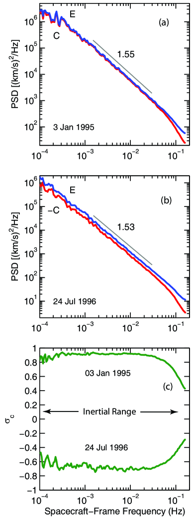
Figure 2: Typical energy $E$ and cross-helicity spectra $C$ (trace spectra) obtained using 3-second plasma velocity and magnetic field data from the Wind spacecraft near the orbit of the earth at 1 AU. (a) An interval of highly Alfvénic high-speed wind from 3 Jan 1995 09:00 to 8 Jan 1995 00:00, 4.625 days. (b) A weak high-speed stream embedded in low-speed wind; 24 Jul 1996 12:00 to 7 Aug 1996 00:00, 14 days. (c) The normalized cross-helicity $\sigma_{c}=C/E$ as a function of frequency. The rapid change in $\sigma_{c}$ near the Nyquist frequency is at least partly caused by the FFT processing techniques and may not be a real physical effect.

which implies that the normalized cross-helicity $\sigma_{c}$ is approximately constant. In other words, the quantity $\sigma_{c}$ is approximately scale invariant. Similar results have been found in simulations of incompressible MHD turbulence (Verma et al., 1996; Perez and Boldyrev, 2009; Beresnyak and Lazarian, 2008). In particular, the 3D simulations of Perez & Boldyrev (Perez and Boldyrev, 2009) indicate that the perpendicular Elsasser spectra are proportional to each other in Fourier space. Solar wind observations also suggest that the probabilities $p$ and $q$ are approximately scale invariant as shown in Fig. 3. These observations will now be taken into account in the theory.

Assuming $\sigma_{c}$ and $p$ are both scale invariant quantities, then $w^{+}/w^{-}$, $v_{\uparrow}/v_{\downarrow}$, $\tau^{+}/\tau^{-}$, and $\theta_{\downarrow}/\theta_{\uparrow}$ are scale invariant by equations (25), (24), (34), and (32), respectively. In all, there are six different scale invariant ratios in the theory

$$\frac{w^{+}}{w^{-}},\quad\frac{\varepsilon^{+}}{\varepsilon^{-}},\quad\frac{p}{q},\quad\frac{v_{\uparrow}}{v_{\downarrow}},\quad\frac{\tau^{+}}{\tau^{-}},\quad\frac{\theta_{\uparrow}}{\theta_{\downarrow}}.$$ (35)

At most, only three of these are independent, say, the first three. Equations (24), (34), and (32) imply

$$\frac{v_{\uparrow}}{v_{\downarrow}}=\sqrt{\frac{q}{p}}\cdot\frac{w^{+}}{w^{-}},$$ (36)

$$\frac{\tau^{+}}{\tau^{-}}=\left(\frac{w^{+}}{w^{-}}\right)^{2}\frac{\varepsilon^{-}}{\varepsilon^{+}},$$ (37)

$$\frac{\theta_{\downarrow}}{\theta_{\uparrow}}=\sqrt{\frac{q}{p}}\left(\frac{w^{+}}{w^{-}}\right)^{3}\frac{\varepsilon^{-}}{\varepsilon^{+}}.$$ (38)

Therefore, the six scale invariant ratios (35) can all be expressed in terms of the first three $w^{+}/w^{-}$, $\varepsilon^{+}/\varepsilon^{-}$, and $p/q$.

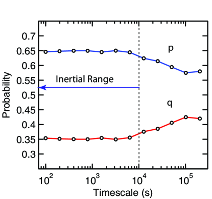
Figure 3: The probabilities $p$ and $q$ obtained from solar wind data by integrating the observed probability density function for the angle $\theta$ from 0 to $\pi/2$ and from $\pi/2$ to $\pi$, respectively. The data was acquired by the Wind spacecraft between 8 Jan 1997 and 9 June 1997 and analyzed using the techniques described in (Podesta et al., 2009). Examples of the probability density functions can be found in (Podesta et al., 2009).

To be able to solve Kolmogorov’s relations (34) for $w^{\pm}$ it is necessary to express the alignment angle $\theta_{\uparrow}$ in terms of $w^{\pm}$. In general, $\theta_{\uparrow}$ can depend on $w^{+}$, $w^{-}$, the Alfvén speed $v_{A}$, the lengthscale $\lambda_{\perp}$, the cascade rates $\varepsilon^{+}$ and $\varepsilon^{-}$, and the probabilities $p$ and $q$. By dimensional analysis, $\theta_{\uparrow}$ must be a function of the following six dimensionless quantities

$$\frac{w^{+}}{v_{A}},\quad\frac{w^{-}}{v_{A}},\quad\frac{\varepsilon^{+}\lambda_{\perp}}{v_{A}^{3}},\quad\frac{\varepsilon^{-}\lambda_{\perp}}{v_{A}^{3}},\quad p,\quad q.$$ (39)

Moreover, $\theta_{\uparrow}$ must change into $\theta_{\downarrow}$ when $w^{+}$, $\varepsilon^{+}$, and $p$ are interchanged with $w^{-}$, $\varepsilon^{-}$, and $q$, respectively, to be consistent with the nonlinear terms (28) and (29). For a theory composed of power law functions, the only forms that satisfy all these requirements are

$$\theta_{\uparrow} \propto\bigg{(}\frac{w^{+}}{v_{A}}\bigg{)}^{\!\alpha}\bigg{(}\frac{w^{-}}{v_{A}}\bigg{)}^{\!\beta}\bigg{(}\frac{\varepsilon^{+}\lambda_{\perp}}{v_{A}^{3}}\bigg{)}^{\!\gamma}\bigg{(}\frac{\varepsilon^{-}\lambda_{\perp}}{v_{A}^{3}}\bigg{)}^{\!\delta}p^{\mu}q^{\nu},$$ (40)

$$\theta_{\downarrow} \propto\bigg{(}\frac{w^{-}}{v_{A}}\bigg{)}^{\!\alpha}\bigg{(}\frac{w^{+}}{v_{A}}\bigg{)}^{\!\beta}\bigg{(}\frac{\varepsilon^{-}\lambda_{\perp}}{v_{A}^{3}}\bigg{)}^{\!\gamma}\bigg{(}\frac{\varepsilon^{+}\lambda_{\perp}}{v_{A}^{3}}\bigg{)}^{\!\delta}q^{\mu}p^{\nu},$$ (41)

where $\alpha$, $\beta$, $\gamma$, $\delta$, $\mu$, and $\nu$ are constants that must be determined by the theory. In addition, there is a leading coefficient which is omitted.

The substitution of (40) and (41) into equation (38) yields $\beta=\alpha+3$, $\delta=\gamma-1$, and $\nu=\mu-1/2$. The parameters are further constrained by considering the geometry of the “turbulent eddies” associated with the fluctuations $v_{\uparrow}$ and $v_{\downarrow}$. The parallel correlation length is defined by $\lambda_{\parallel}^{\uparrow}=v_{A}\tau_{\uparrow}$ and the correlation length in the direction of the velocity fluctuation is $\bm{\xi}_{\uparrow}=\bm{v}_{\uparrow}\tau_{\uparrow}$. Similarly, the correlation lengths for negatively aligned fluctuations are $\lambda_{\parallel}^{\downarrow}=v_{A}\tau_{\downarrow}$ and $\xi_{\downarrow}=v_{\downarrow}\tau_{\downarrow}$. In the plane perpendicular to the local mean magnetic field $\bm{\xi}$ is parallel to $\bm{v}$, the gradient direction is perpendicular to $\bm{v}$ with lengthscale $\lambda_{\perp}$, and the eddy dimensions are $\xi\times\lambda_{\perp}$. The dimension parallel to the mean magnetic field is $\lambda_{\parallel}$. Hence, in physical space the turbulent eddies can be visualized as three-dimensional structures with dimensions $\lambda_{\perp}\times\xi\times\lambda_{\parallel}$.

The coherence times for longitudinal and transverse motions of the eddy must be equal to each other and also to the cascade time. This is the critical balance condition of Goldreich and Sridhar which is also implicit in the work of Higdon Higdon (1984). Equation (33) and the definitions of the correlation lengths in the last paragraph immediately yield the critical balance condition

$$\tau_{\uparrow}=\frac{\lambda_{\parallel}^{\uparrow}}{v_{A}}=\frac{\xi_{\uparrow}}{v_{\uparrow}}\simeq\frac{\lambda_{\perp}}{2v_{\uparrow}\theta_{\uparrow}}$$ (42)

with a similar condition for the negatively aligned fluctuations

$$\tau_{\downarrow}=\frac{\lambda_{\parallel}^{\downarrow}}{v_{A}}=\frac{\xi_{\downarrow}}{v_{\downarrow}}\simeq\frac{\lambda_{\perp}}{2v_{\downarrow}\theta_{\downarrow}}.$$ (43)

Now consider the eddy geometry. When the mean magnetic field is strong enough that $w^{\pm}/v_{A}<1$, then $\lambda_{\parallel}>\xi>\lambda_{\perp}$ and the eddies are elongated in the parallel direction. The condition $w^{\pm}/v_{A}<1$ is assumed hereafter. Equation (42) shows that the aspect ratio in the field perpendicular plane is $\phi_{\uparrow}=\lambda_{\perp}/\xi_{\uparrow}=2\theta_{\uparrow}$ and the aspect ratio in the parallel direction is, from equations (42) and (20),

$$\psi_{\uparrow}=\frac{\xi_{\uparrow}}{\lambda_{\parallel}^{\uparrow}}=\frac{v_{\uparrow}}{v_{A}}=\frac{w^{+}}{2v_{A}p^{1/2}}.$$ (44)

The two aspect ratios will scale in the same way if $\phi_{\uparrow}/\psi_{\uparrow}$ is scale invariant. This implies that $\alpha=-1$ and $\gamma=1/2$. The assumption that the ratio $\phi_{\uparrow}/\psi_{\uparrow}$ is scale invariant is different from Boldyrev’s original approach in which he assumed that the alignment angles in and out of the field perpendicular plane are simultaneously minimized. Nevertheless, our assumption retains the spirit of Boldyrev’s original theory which implies the geometry of turbulent fluctuations are scale-invariant.

Solving Kolmogorov’s relation (34) using (32), (40), (41), and the parameter values obtained so far, one finds

$$\frac{w^{\pm}}{v_{A}}\simeq\bigg{(}\frac{w^{+}}{w^{-}}\bigg{)}^{\!\pm 1/2}\bigg{(}\frac{\varepsilon^{-}}{\varepsilon^{+}}\bigg{)}^{\!\pm 1/8}\bigg{(}\frac{\varepsilon^{\pm}\lambda_{\perp}}{v_{A}^{3}}\bigg{)}^{\!1/4}(pq)^{-\nu/4}$$ (45)

and the total energy cascade rate $\varepsilon=(\varepsilon^{+}+\varepsilon^{-})/2$ is

$$\varepsilon=\frac{(w^{+}w^{-})^{2}}{4v_{A}\lambda_{\perp}}\Bigg{(}\sqrt{\frac{\varepsilon^{+}}{\varepsilon^{-}}}+\sqrt{\frac{\varepsilon^{-}}{\varepsilon^{+}}}\Bigg{)}(pq)^{\nu}.$$ (46)

The total energy at scale $\lambda_{\perp}$ is

$$\frac{(w^{+})^{2}+(w^{-})^{2}}{4}=\frac{w^{+}w^{-}}{4}\bigg{(}\frac{w^{+}}{w^{-}}+\frac{w^{-}}{w^{+}}\bigg{)}\equiv v^{2}.$$ (47)

Therefore, the energy cascade rate can be written

$$\epsilon=\frac{4v^{4}}{v_{A}\lambda_{\perp}}\Bigg{(}\sqrt{\frac{\varepsilon^{+}}{\varepsilon^{-}}}+\sqrt{\frac{\varepsilon^{-}}{\varepsilon^{+}}}\Bigg{)}\bigg{(}\frac{w^{+}}{w^{-}}+\frac{w^{-}}{w^{+}}\bigg{)}^{\!-2}(pq)^{\nu}.$$ (48)

Assuming the rms energy $v^{2}$ at scale $\lambda_{\perp}$ is held constant, the terms on the right-hand side describe the dependence of the energy cascade rate on the ratios $\varepsilon^{+}/\varepsilon^{-}$ and $w^{+}/w^{-}$. The value of $\nu$ may be determined by comparison with experiment or possibly by further physical considerations. This parameter does not affect the inertial range scaling laws and is left undetermined for the moment.

At this point it is of interest to return to the expressions (32) for the cascade times and ask: How do the cascade times depend on the rms Elsasser amplitudes? Using the parameter values obtained previously, equation (40) becomes

$$\theta_{\uparrow}\sim\bigg{(}\frac{w^{+}}{v_{A}}\bigg{)}^{\!-1}\bigg{(}\frac{w^{-}}{v_{A}}\bigg{)}^{\!2}\bigg{(}\frac{\varepsilon^{+}\lambda_{\perp}}{v_{A}^{3}}\bigg{)}^{\!1/2}\bigg{(}\frac{\varepsilon^{-}\lambda_{\perp}}{v_{A}^{3}}\bigg{)}^{\!-1/2}p^{\nu+1/2}q^{\nu}$$ (49)

and the substitution of this result into equation (32) yields

$$\tau^{+}\simeq\frac{\lambda_{\perp}}{v_{A}}\bigg{(}\frac{v_{A}}{w^{-}}\bigg{)}^{\!2}\bigg{(}\frac{\varepsilon^{-}}{\varepsilon^{+}}\bigg{)}^{\!1/2}(pq)^{-\nu}.$$ (50)

A similar expression holds for $\tau^{-}$ so that the ratio $\tau^{+}/\tau^{-}$ satisfies (37). Ignoring scale invariant factors, the preceding equation shows that

$$\tau^{+}\propto\frac{\lambda_{\perp}v_{A}}{(w^{-})^{2}}\qquad\mbox{and}\qquad\tau^{-}\propto\frac{\lambda_{\perp}v_{A}}{(w^{+})^{2}}.$$ (51)

In this form, the angle dependence has been eliminated. Note that the simple estimate $\tau^{+}\sim\lambda_{\perp}/w^{-}$ suggested by the nonlinear term in the MHD equations is modified by the factor $v_{A}/w^{-}$ which accounts for the weakening of nonlinear interactions caused by scale dependent alignment. The presence of this algebraic factor is one of the hallmarks of Boldyrev’s original (2006) theory which is generalized here to imbalanced turbulence. Remarkably, the relations (51) are identical to those in the isotropic theory of imbalanced turbulence developed by Dobrowolny, Mangeney, and Veltri; see equation (10) in (Dobrowolny et al., 1980). Recall that Dobrowolny, Mangeney, and Veltri concluded from their expressions for the cascade times that steady state turbulence with nonvanishing cross-helicity is impossible. On the contrary, the theory presented here allows such a steady state because the additional coefficients shown in (50) but not (51) maintain the relation (37) even when $\varepsilon^{+}\neq\varepsilon^{-}$. Thus, the theory presented here is also a generalization of the theory of Dobrowolny, Mangeney, and Veltri (Dobrowolny et al., 1980).

A remark about the timescales in the theory should be mentioned. If $w^{+}>w^{-}$, then equation (37) implies it is possible that $\tau^{+}<\tau^{-}$ since there is nothing in the theory that prevents this. That is, the energy of the more energetic Elsasser species may be transferred to smaller scales in less time than the energy of the less energetic Elsasser species. This is not inconsistent with dynamic alignment, a well known effect seen in simulations of decaying incompressible MHD turbulence where the minority species usually decays more rapidly than the dominant species causing the magnitude of the normalized cross-helicity to increase with time (Dobrowolny et al., 1980; Matthaeus et al., 1983; Matthaeus and Montgomery, 1984; Pouquet et al., 1986).

In freely decaying turbulence, dynamic alignment occurs whenever the total energy decays more rapidly than the cross-helicity, that is, $\varepsilon>|\varepsilon_{c}|$, where the cascade rate of cross-helicity $\varepsilon_{c}$ may be positive or negative. From the relations $\varepsilon>0$ and $\varepsilon^{\pm}=\varepsilon\pm\varepsilon_{c}$, it follows that dynamic alignment occurs if and only if $\varepsilon^{+}>0$ and $\varepsilon^{-}>0$. If $w^{+}>w^{-}$, it is not necessary that $\tau^{+}>\tau^{-}$, only that

$$\frac{\tau^{+}}{\tau^{-}}>\frac{\varepsilon^{-}}{\varepsilon^{+}},$$ (52)

as can be seen from equation (37). Therefore, even though the relation $\tau^{+}<\tau^{-}$ may seem counter-intuitive, it is not inconsistent with dynamic alignment.

V Summary and Conclusions

Observations of scale dependent alignment of velocity and magnetic field fluctuations $\delta\bm{v}_{\perp}$ and $\delta\bm{b}_{\perp}$ in the solar wind suggest that this effect must be included in any theory of solar wind turbulence (Podesta et al., 2008, 2009). Perez and Boldyrev (2009) have recently discussed a theory of imbalanced turbulence that includes scale dependent alignment of the fluctuations $\delta\bm{v}_{\perp}$ and $\delta\bm{b}_{\perp}$ in the inertial range. We have extended the Perez-Boldyrev theory by including the probabilities $p$ and $q$ which solar wind observations indicate are not necessarily equal. Operationally, the probabilities $p$ and $q$ may be defined as follows. Suppose space is covered by a uniform cartesian grid or three dimensional mesh. At each grid-point one may compute the fluctuations $\delta\bm{v}_{\perp}$ and $\delta\bm{b}_{\perp}$ and the angle between them $\theta$. If the angle lies in the range $0<\theta<\pi/2$, then the fluctuation is positively aligned and if $\pi/2<\theta<\pi$, then the fluctuation is negatively aligned. By counting the number of positively and negatively aligned fluctuations in a large volume $V$, much larger than the lengthscales of the turbulent eddies, the probabilities $p$ and $q$ may be defined as the fractional numbers of positively and negatively aligned fluctuations in the volume $V$.

The phenomenological theory developed in this paper was guided primarily by two new solar wind observations. It should be noted that both of these solar wind observations are necessary for the development of the theory. At first glance, it may seem that the condition $\sigma_{c}=$ const implies that $p$ and $q$ are both constant. Or that these two conditions are somehow equivalent. However, the relation $(w^{+}/w^{-})^{2}\simeq pv_{\uparrow}^{2}/qv_{\downarrow}^{2}$, equation (24), shows that $p/q$ can vary with the lengthscale even if $w^{+}/w^{-}$ is constant. Therefore, it is essential to have separate observations of the scale invariance of $\sigma_{c}$ and the scale invariance of $p$ and $q$ to support the theoretical framework developed here.

In summary, using estimates of the cascade times derived from the nonlinear terms in the incompressible MHD equations and two new observational constraints derived from studies of solar wind data, we have constructed a generalization of Boldyrev’s theory (Boldyrev, 2006) that depends on the three parameters $w^{+}/w^{-}$, $\varepsilon^{+}/\varepsilon^{-}$, and $p/q$. The theory reduces to the original theory of Boldyrev (2006) when $w^{+}=w^{-}$, $\epsilon^{+}=\epsilon^{-}$, and $p=q$ since in this limit $\theta_{\uparrow}=\theta_{\downarrow}$ and the cascade times (32) become equal to those of Boldyrev (2006). For imbalanced turbulence $w^{+}\neq w^{-}$, $p\neq q$, and the theory predicts the scaling laws $w^{\pm}\propto\lambda_{\perp}^{1/4}$, $\theta_{\uparrow\downarrow}\propto\lambda_{\perp}^{1/4}$, and $\lambda_{\parallel}^{\pm}\propto\lambda_{\perp}^{1/2}$. Interestingly, the scaling laws for balanced and imbalanced turbulence are the same. The perpendicular energy spectrum defined by $k_{\perp}E^{\pm}\sim|w^{\pm}|^{2}$ has the inertial range scaling $E^{\pm}\propto k_{\perp}^{-3/2}$ with

$$\frac{E^{+}}{E^{-}}=\bigg{(}\frac{w^{+}}{w^{-}}\bigg{)}^{\!2}=\frac{1+\sigma_{c}}{1-\sigma_{c}}=\mbox{const}.$$ (53)

The theory assumes that the cascades for positively and negatively aligned fluctuations are both in a state of critical balance (42), although they are governed by different timescales, and that the eddy geometry is scale invariant. The positively aligned fluctuations occupy a fractional volume $p$ and the negatively aligned fluctuations occupy a fractional volume $q$ so that the energy cascade rate is

$$\varepsilon=p\frac{v_{\uparrow}^{2}}{\tau_{\uparrow}}+q\frac{v_{\downarrow}^{2}}{\tau_{\downarrow}}$$ (54)

or, equivalently,

$$\varepsilon=\frac{(w^{+})^{2}}{4\tau^{+}}+\frac{(w^{-})^{2}}{4\tau^{-}}.$$ (55)

In the discussion following equation (35) it was shown that at most three of the ratios $w^{+}/w^{-}$, $\varepsilon^{+}/\varepsilon^{-}$, and $p/q$ can be independent. However, the two ratios $w^{+}/w^{-}$ and $\varepsilon^{+}/\varepsilon^{-}$ cannot be independent since in the case of homogeneous steady-state turbulence $w^{+}=w^{-}$ implies $\varepsilon^{+}=\varepsilon^{-}$ and vice versa. This is because the injection of cross-helicity into the system, $\varepsilon_{c}\neq 0$ or $\varepsilon^{+}\neq\varepsilon^{-}$, will create a nonzero cross-helicity spectrum and a cascade of cross-helicity from large to small scales which implies a net accumulation of cross-helicity within the volume ($\sigma_{c}\neq 0$). Hence, at most two of the ratios and $w^{+}/w^{-}$ and $p/q$ are independent. Whether $p/q$ can be expressed in terms of $w^{+}/w^{-}$ and $\varepsilon^{+}/\varepsilon^{-}$ is an open question.