Multidimensional thermodynamic potential for descriptions of ultrathin lubricant film melting
between two atomically smooth surfaces

Abstract

The thermodynamic model of ultrathin lubricant film melting, confined between two atomically-flat solid surfaces, is built using the Landau phase transition approach. Non-equilibrium entropy is introduced describing the part of thermal motion conditioned by non-equilibrium and non-homogeneous character of the thermal distribution. The equilibrium entropy changes during the time of transition of non-equilibrium entropy to the equilibrium subsystem. To describe the condition of melting, the variable of the excess volume (disorder parameter) is introduced which arises due to chaotization of a solid structure in the course of melting. The thermodynamic and shear melting is described consistently. The stick-slip mode of melting, which is observed in experiments, are described. It is shown that with growth of shear velocity, the frequency of stiction spikes in the irregular mode increases at first, then it decreases, and the sliding mode comes further characterized by the constant value of friction force. Comparison of the obtained results with experimental data is carried out. boundary friction, nanotribology, dynamic modelling, shear stress and strain, viscoelastic medium, stick-slip mode 05.70.Ce, 05.70.Ln, 47.15.gm, 62.20.Qp, 64.60.-i, 68.35.Af

Abstract

В межах теорiї фазових переходiв Ландау побудовано термодинамiчну модель плавлення ультратонкої плiвки мастила, що затиснута мiж двома атомарно-гладкими твердими поверхнями. Введено нерiвноважну ентропiю, що описує частину теплового руху, який обумовлений нерiвноважним i нерiвномiрним характером теплового розподiлу. Рiвноважна ентропiя змiнюється у часi за рахунок переходу нерiвноважної ентропiї в рiвноважну пiдсистему. Для опису стану мастила введено параметр надлишкового об’єму (параметр безладу), який виникає унаслiдок хаотизацiї структури твердого тiла в процесi плавлення. Узгодженим чином описано термодинамiчне i зсувне плавлення. Описано переривчастий режим плавлення, який спостерiгається в експериментах. Показано, що iз зростанням швидкостi зсуву частота пiкiв прилипання в переривчастому режимi спочатку збiльшується, потiм зменшується, i далi наступає режим ковзання, що характеризується постiйним значенням сили тертя. Проведено порiвняння отриманих результатiв з експериментальними даними. межове тертя, нанотрибологiя, динамiчне моделювання, зсувнi напруження та деформацiя, в’язкопружне середовище, переривчастий режим

1 Introduction

With the development of nanotechnologies, the friction of two smooth solid surfaces at the presence of thin lubricant film between them has been vastly investigated lately [1]. Experimental study of atomically-flat surfaces of mica, which are separated by ultrathin layer of lubricant, shows that lubricant has properties of solid at certain conditions [2]. In particular, the interrupted motion (stick-slip) inherent in a dry friction [3, 4] is observed. Such boundary mode is realized, if the film of lubricating material has less than four molecular layers, and this is explained as solidification conditioned by compression of walls. The subsequent jump-like melting takes place, when shear stress exceeds a critical value due to the effect of ‘‘shear melting’’.

In a general case, the description of behavior of ultrathin lubricant film should be carried out starting with the first principles. However, such an approach is complicated due to different lubricants and geometry of experiment used. Therefore, the phenomenological models are proposed that allow us to explain the experimentally observed results. In particular, thermodynamic [5], mechanistic [6, 7, 8], and synergetic [9] models are built. They are of deterministic [6, 9] and stochastic [7, 8] nature. Also, the studies are carried out using methods of molecular dynamics [10, 11, 12, 13]. It appears that the lubricant can provide several kinetic modes [2], between which transitions occur stipulating the interrupted friction [2, 4]. In work [7] three modes of friction are revealed at the account of stochastic effects: sliding mode that is inherent in low-velocity shear, regular interrupted mode, and mode of sliding at high-velocity shear. The existence of these modes is also confirmed by the synergetic theory taking into account the deformation defect of the shear modulus of lubricant [14] and the computer experiments [1, 2, 3, 15].

In work [9] within the framework of the Lorenz model for approximation of viscoelastic medium, the approach is developed according to which the transition of ultrathin lubricant film from the solid-like state to the liquid-like state takes place as a result of thermodynamic and shear melting. An analytical description of these phenomena was presented under the assumption that they are the results of shear stress and strain self-organization as well as of the lubricant temperature. Additive noises of the indicated quantities [16, 17, 18] and correlated fluctuations of temperature [19] are taken into account. The reasons for the jump-like melting and hysteresis, which are observed in experiments [20, 21, 22], are considered in works [14, 23, 24]. Three stationary modes are found out: two solid-like, inherent in the dry friction, and liquid-like, corresponding to sliding. It is shown that transition between two last modes takes place in accordance with hysteresis of the dependence of stress on strain (at the jump-like melting) or on the temperature of friction surfaces.

At the same time, the traditional use of the Lorenz equations set for the above problem leads to logical contradictions already at the stage of formulation of the problem. Consideration of strain and stress as independent quantities, i.e., that for each of them a separate kinetic equation is written, contradicts the canons of ‘‘classic’’ mechanics and thermodynamics. Moreover, there is no symmetry of types of thermodynamic flows at such formulation which predetermines strict accordance of signs in the mixed terms in kinetic equations. An output can be found using a multidimensional thermodynamic potential from which the set of Landau-like kinetic equations must follow by standard procedure of differentiation [25]. Earlier this approach was applied for description of the processes of severe plastic deformation (SPD) [26, 27, 28] and fracture of quasibrittle solids [29]. The latest advances and statistical justification of this approach are outlined in works [30, 31, 32]. Both the process of SPD and the process of ultrathin lubricant sliding have a lot in common, which allows us to claim the legitimacy of application of such a technique in both cases. However, principal differences between these processes are present. They are mainly related to an ultrathin thickness of lubricant layer (order of atomic size), which brings in the limitations and deviations from standard procedure, which we shall consider in the proper place of the article.

The general thermodynamic model of ultrathin lubricant film melting is built in the offered work. Kinetic equations are written in as Landau-Khalatnikov ones for basic parameters (section 2). In section 3 the effect of shear velocity is considered and it is shown that there exists a critical value of velocity, at which lubricant melts in accordance with the mechanism of shear melting. The effect of temperature is investigated. It is shown that at temperature exceeding its critical value, the lubricant can melt even at the zero applied shear stress and at zero velocity of the shearing, i.e., the thermodynamic melting takes place (section 4). The effect of fluctuations of the strain is analyzed which arise due to errors in the experimental setup (section 5). All of the found features coincide with the ones for experimental data.

2 Thermodynamic model

At the construction of a model within the framework of the Landau theory of phase transitions [25], at first, it is necessary to choose a parameter whose values characterize the examined phases. This parameter is called an order parameter and describes a change of phase symmetry at the phase transition point. An order parameter changes discontinuously during the first-order phase transitions and it varies smoothly during the second-order phase transitions. However, the phase symmetry changes discontinuously at the phase transition point in both cases. A phase becomes more ordered with the growth of the order parameter and symmetry falls down.

Melting of a thin lubricant film unlike melting of volume medium can take place according to the scenario of second-order phase transition [5]. However, there is a certain problem at describing the states of thin lubricant films, because such films demonstrate more than one type of transition [2]. States of a lubricant film are not true thermodynamic phases. They are interpreted as kinetic modes of friction [4]. Therefore, one speaks not about a solid and a liquid, but about a solid-like and a liquid-like phases. The increase in volume [10] and diffusion coefficient [10, 11, 33, 34] of such lubricants shows the melting process. Since the volume is experimentally observable, to describe the state of lubricant, a parameter $f$ is introduced, which also relates to the order parameter (a disorder parameter [35]). It has a physical meaning of an excess volume, arising due to the chaotization (the amorphization) of structure of a solid during the process of melting. The excess volume acquires zero value at zero Kelvin, when all atoms of the system are densely packed at rest. It is different from zero both in the solid and in the liquid state at non-zero temperature. However, it has a larger value in the liquid state. We introduce two values of this parameter: at $f>f_{\rm liq}$ lubricant is liquid-like, and when $f<f_{\rm sol}$, it solidifies, and the symmetry of state is decreased.

Now, in accordance with general procedure, it is necessary to write down an expansion of energy in the independent variables. Internal energy for a model, in which both contributions of large shear strain $\varepsilon_{ij}^{\rm e}$ and of entropy $s$ and nonequilibrium entropy $\tilde{s}$ are taken into account simultaneously, is written as [28]:

$$u=u_{0}+t_{0}\tilde{s}-\frac{1}{2}t_{1}\tilde{s}^{2}+\varphi_{0}f-\frac{1}{2}\varphi_{1}f^{2}-m_{1}\tilde{s}f,$$ (1)

where

$$u_{0} = \frac{1}{2}\lambda\left(\varepsilon_{ii}^{\rm e}\right)^{2}+\mu\left(\varepsilon_{ij}^{\rm e}\right)^{2}+\alpha s^{2}+\beta s\varepsilon_{ii}^{\rm e}\,,$$ (2)

$$t_{0} = X_{3}^{(0)}\varepsilon_{ii}^{\rm e}+X_{6}^{(0)}\left(\varepsilon_{ij}^{\rm e}\right)^{2}+\alpha_{t}s,$$ (3)

$$\varphi_{0} = g\varepsilon_{ii}^{\rm e}+\bar{\mu}\left(\varepsilon_{ij}^{\rm e}\right)^{2}+\alpha_{\varphi}s,$$ (4)

$$\varphi_{1} = \varphi_{1}^{\ast}+\tilde{\mu}\left(\varepsilon_{ij}^{\rm e}\right)^{2},$$ (5)

$$m_{1} = m_{1}^{\ast}+X_{3}\varepsilon_{ii}^{\rm e}+X_{6}\left(\varepsilon_{ij}^{\rm e}\right)^{2}$$ (6)

and $\lambda$, $\mu$, $\alpha$, $\beta$, $X_{3}^{(0)}$, $X_{6}^{(0)}$, $\alpha_{t}$ , $g$, $\bar{\mu}$ , $\alpha_{\varphi}$ , $\varphi_{1}^{\ast}$ , $\tilde{\mu}$ , $m_{1}^{\ast}$ , $X_{3}$ , $X_{6}$ are constants of expansion.

Elastic stresses are taken into account with accuracy to quadratic contributions via the first two invariants of the strain tensor $\varepsilon_{ii}^{\rm e}$ , $(\varepsilon_{ij}^{\rm e})^{2}=\varepsilon_{ij}^{\rm e}\varepsilon_{ji}^{\rm e}$ , where summing is implied over repeated pairs of indices. Thus, the first invariant represents the trace of the strain tensor $\varepsilon_{ii}^{\rm e}=\varepsilon_{1}^{\rm e}+\varepsilon_{2}^{\rm e}+\varepsilon_{3}^{\rm e}$ , the second one is determined by expression [36]

$$(\varepsilon_{ij}^{\rm e})^{2}\equiv(\varepsilon_{ll}^{\rm e})^{2}-2I_{2}=(\varepsilon_{1}^{\rm e})^{2}+(\varepsilon_{2}^{\rm e})^{2}+(\varepsilon_{3}^{\rm e})^{2}.$$ (7)

These determinations of invariants suppose that symmetric tensor $\varepsilon_{ij}^{\rm e}$ of elastic strain is transformed to the diagonal form.

A new basic quantity, i.e., the non-equilibrium entropy $\tilde{s}$, is introduced here describing the part of thermomotion, which is conditioned by non-equilibrium character of the thermal distribution. Exactly this part of the entropy is produced owing to dynamic transition processes at generation of the free volume during external action, tending to some stationary value [26, 27, 28, 29, 30, 31]. The equilibrium entropy does not evolve in the ordinary understanding, but changes with time due to relaxation of non-equilibrium entropy and its transition into the equilibrium subsystem.

We write down the corresponding kinetic equations for non-equilibrium parameters of state $X_{i}$ in the form

$$\tau_{X_{i}}\dot{X}_{i}=\frac{\partial u}{\partial X_{i}}\,,$$ (8)

where $\tau_{X_{i}}$ are the relaxation times.

At description by equations (8), the system tends to a maximum of the internal energy that corresponds to strongly non-equilibrium processes occurring in open systems at energy pumping therein (strictly speaking, this is true for an ‘‘effective’’ internal energy, which is a combination of the internal energy and the entropic factor [32]). For example, the maximum of internal energy is of crucial importance for magnetic [37] and for alloy orderings [38, 39]. This property of the internal energy is also similar to the property of thermodynamic potential, introduced earlier for strongly non-equilibrium processes [40]. In our case, the energy pumping is realized due to deformation at the displacement of the friction surfaces. Thus, a kinetic equation for the excess volume assumes the form

$$\tau_{f}\frac{\partial f}{\partial t}=\varphi_{0}-\varphi_{1}f-m_{1}\tilde{s},$$ (9)

and for the non-equilibrium entropy $\tilde{s}$ we obtain

$$\tau_{s}\frac{\partial\tilde{s}}{\partial t}=t_{0}-t_{1}\tilde{s}-m_{1}f,$$ (10)

where the terms with the sign ‘‘+’’ describe the increase in non-equilibrium entropy due to the external source of energy (the work), the terms with the sign ‘‘–’’ reflect its drift to the equilibrium subsystem.

The kinetic equations for the equilibrium entropy differs from the usual form (8), since a change of equilibrium entropy occurs due to transition of its non-equilibrium form to equilibrium one.

In the case of non-homogeneous heating, the equation of heat conductivity represents the ordinary equation of continuity [41]:

$$T\frac{\partial s}{\partial t}=\kappa\nabla^{2}T,$$ (11)

where coefficient of heat conductivity $\kappa$ is a constant. Supposing that a layer of lubricant and atomically-flat surfaces have different temperatures $T$ and $T_{\rm e}$ accordingly, for a normal constituent $\nabla^{2}_{z}$ it is possible to use the approximation with sufficient accuracy $\kappa\nabla^{2}_{z}T\approx(\kappa/h^{2})(T_{\rm e}-T)$, where $h$ is the thickness of lubricant. Taking this into account, equation (11) is written down in a simple form

$$\frac{\partial s}{\partial t}=\frac{\kappa}{h^{2}}\left(\frac{T_{\rm e}}{T}-1\right),$$ (12)

where quantity $h^{2}/\kappa$ plays the role of relaxation time, during which an equalization of the temperature occurs over the thickness of the lubricant due to usual heat conductivity.

The decrease in the non-equilibrium entropy is taken into account by the negative terms in the kinetic equation (10), which means that the same terms with positive sign must be taken into account in the equilibrium entropy. Therefore, the final kinetic equation for the equilibrium entropy is written down in the form:

$$\tau_{s}\frac{\partial s}{\partial t}=t_{1}\tilde{s}+m_{1}f+\frac{\tau_{s}\kappa}{h^{2}}\left(\frac{T_{\rm e}}{T}-1\right).$$ (13)

In accordance with the expression for the internal energy, the temperature of the lubricant is obtained in the form:

$$T=\frac{\partial u}{\partial s}=2\alpha s+\alpha_{t}\tilde{s}+\alpha_{\varphi}f+\beta\varepsilon_{ii}^{\rm e}\,.$$ (14)

According to (1), elastic stresses are determined as $\sigma_{ij}^{\rm e}=\partial u/\partial\varepsilon_{ij}^{\rm e}$ :

$$\sigma_{ij}^{\rm e} = \lambda\varepsilon_{ii}^{\rm e}\delta_{ij}+2\mu\varepsilon_{ij}^{\rm e}+\beta s\delta_{ij}+\left(X_{3}^{(0)}\delta_{ij}+2X_{6}^{(0)}\varepsilon_{ij}^{\rm e}\right)\tilde{s}$$ (15)

$$+ \left(g\delta_{ij}+2\bar{\mu}\varepsilon_{ij}^{\rm e}\right)f-\tilde{\mu}\varepsilon_{ij}^{\rm e}f^{2}-\left(X_{3}\delta_{ij}+2X_{6}\varepsilon_{ij}^{\rm e}\right)\tilde{s}f.$$

Expression (15) can be presented as the effective Hooke law

$$\sigma_{ij}^{\rm e}=\sigma_{\rm v}\delta_{ij}+2\mu_{\rm eff}\varepsilon_{ij}^{\rm e}+\lambda\varepsilon_{ii}^{\rm e}\delta_{ij}$$ (16)

with the effective elastic parameter

$$\mu_{\rm eff}=\mu+X_{6}^{(0)}\tilde{s}+\bar{\mu}f-\frac{1}{2}\tilde{\mu}f^{2}-X_{6}\tilde{s}f\,.$$ (17)

Constants $\mu_{\rm eff}$ and $\lambda$ are the Lame coefficients [41]. The term, being independent of strain, appears in (16)

$$\sigma_{\rm v}=\beta s+X_{3}^{(0)}\tilde{s}+gf-X_{3}\tilde{s}f.$$ (18)

The first and second invariants are determined as

$$\varepsilon_{ii}^{\rm e} = \frac{n-\sigma_{\rm v}}{\lambda+\mu_{\rm eff}}\,,$$ (19)

$$(\varepsilon_{ij}^{\rm e})^{2} \equiv \varepsilon_{ij}^{\rm e}\,\varepsilon_{ji}^{\rm e}=\frac{1}{2}\left[\left(\frac{\tau}{\mu_{\rm eff}}\right)^{2}+\left(\varepsilon_{ii}^{\rm e}\right)^{2}\right],$$ (20)

where $n$, $\tau$ are the normal and tangential components of stresses acting on the lubricant on the part of the rubbing surfaces. The relationships (19) and (20) represent an ordinary connection between the components of tensors and their invariants of linear elasticity theory (see, for example, [36]). Let us use the Debye approximation relating elastic strain $\varepsilon_{ij}^{\rm e}$ with plastic one $\varepsilon_{ij}^{\rm pl}$ [5]:

$$\dot{\varepsilon}_{ij}^{\rm pl}=\frac{\varepsilon_{ij}^{\rm e}}{\tau_{\varepsilon}}\,.$$ (21)

The total strain in a layer is determined as

$$\varepsilon_{ij}=\varepsilon_{ij}^{{\rm e}}+\varepsilon_{ij}^{\rm pl}\,.$$ (22)

This strain fixes the motion velocity of overhead block $V_{ij}$ according to relationship [2]

$$V_{ij}=h\dot{\varepsilon}_{ij}=h(\dot{\varepsilon}_{ij}^{\rm e}+\dot{\varepsilon}_{ij}^{\rm pl}).$$ (23)

Relaxation time of strain in (21) depends on the state of the lubricant:

$$\tau_{\varepsilon}=K(\gamma_{0}-\gamma_{1}f),$$ (24)

where the constants $\gamma_{0}$ , $\gamma_{1}$ and coefficient $K$ are introduced. For the solid-like state of the lubricant $K=K_{\rm sol}$ .

In the solid-like state, $\tau_{\varepsilon}$ is large and, therefore, $\varepsilon_{ij}^{\rm e}$ is large in accordance with the expression (24). For the liquid-like state, $\tau_{\varepsilon}$ is small in comparison with the solid-like case, and $\varepsilon_{ij}^{\rm e}$ is small too. Combining relationships (21)–(24) we obtain an expression for elastic shear strain:

$$\frac{\partial\varepsilon_{ij}^{\rm e}}{\partial t}=-\frac{\varepsilon_{ij}^{\rm e}}{K(\gamma_{0}-\gamma_{1}f)}+\frac{V_{ij}}{h}\,.$$ (25)

The experimental data also evidence that in the liquid-like state, the elastic strains relax rapidly [2] and the relaxation time for a liquid-like state is substantially smaller. The expression (24) at $K=K_{\rm sol}$ already reflects the tendency of the relaxation time to decrease with melting (at increase in $f$), but such a dependence is fulfilled only for the solid-like state and near a transition point [5]. Therefore, it is necessary to assume for the liquid-like lubricant $K=K_{\rm liq}<K_{\rm sol}$ .

It is known that the melting of lubricant is of hysteresis nature in most cases [7, 20, 21, 22]. For theoretical description of the hysteresis phenomena, a series of works were undertaken, in particular, within the framework of Lorenz model [14, 23, 24]. In this approach, to account for the indicated phenomena, it is necessary to select two characteristic values of the excess volume: at $f>f_{\rm liq}$ lubricant is liquid-like, and when $f<f_{\rm sol}$ it solidifies.

Let us get an expression for the friction force that is measured in experiments [2]. Besides the elastic stresses $\sigma_{ij}^{\rm e}$, the viscous ones $\sigma_{ij}^{\rm visc}$ also arise in the lubricant. The total stress in a layer is the sum of these two contributions

$$\sigma_{ij}=\sigma_{ij}^{\rm e}+\sigma_{ij}^{\rm visc}\,.$$ (26)

The total friction force is determined in a standard manner:

$$F_{ij}=\sigma_{ij}A,$$ (27)

where $A$ is an area of contact. The viscous stresses in a layer are given by the expression [42]

$$\sigma_{ij}^{\rm visc}=\frac{\eta_{\rm eff}V_{ij}}{h}\,,$$ (28)

where $\eta_{\rm eff}$ is the effective viscosity that is defined only experimentally, and for the boundary mode [42]

$$\eta_{\rm eff}\sim\left(\dot{\varepsilon}_{ij}\right)^{\gamma}.$$ (29)

Taking into account (23), (29), the expression for the viscous stresses (28) is written down in the form:

$$\sigma_{ij}^{\rm visc}=\left(\frac{V_{ij}}{h}\right)^{\gamma+1}.$$ (30)

Putting (26), (30) in (27), we obtain the final expression for the friction force:

$$F_{ij}=\left[\sigma_{ij}^{\rm e}+\left(\frac{V_{ij}}{h}\right)^{\gamma+1}\right]A,$$ (31)

where $\sigma_{ij}^{\rm e}$ is fixed by the expression (16) at $i\neq j$.

3 The effect of velocity and shear melting

Ultrathin lubricant films behave differently from volume medium. Therefore, at their description it is impossible to use standard formalism without changes, since a number of principal new effects appear, which must be taken into account. One of them is an interrupted motion (stick-slip) [2, 4] schematically shown in figure 1.

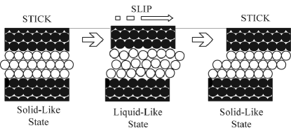
Figure 1: Schematic realization of the interrupted (stick-slip) friction mode [2].

At the beginning, the lubricant is solid-like (stick), but after exceeding some critical value of the elastic shear stress $\sigma_{ij}^{\rm e}$ it rapidly transforms into the liquid-like phase (slip) due to disordering. The top rubbing surface climbs, because a change of lubricant volume takes place. The relaxation of $\sigma_{ij}^{\rm e}$ occurs in the liquid-like state and the lubricant solidifies again (stick) due to the compression by the walls under the action of a load. This process is periodic. One of the basic differences from the behavior of volume lubricants in this mechanism is that the action of the shear stress $\sigma_{ij}^{\rm e}$ causes not only a shear but also an increase in lubricant volume. This fact agrees with the results, which are obtained using the methods of molecular dynamics [10], and can be reflected by modifying the expression (19) as follows:

$$\varepsilon_{ii}^{\rm e}=\frac{n-\sigma_{\rm v}+\sigma_{ij}^{\rm e}\,\varepsilon_{ij}^{\rm a}}{\lambda+\mu_{\rm eff}}\,.$$ (32)

The dimensionless tensor constant $\varepsilon_{ij}^{\rm a}$ is introduced here, which fixes the dilatation power (the expansion of lubricant at a shear under the action of $\sigma_{ij}^{\rm e}$). Thus, it is also necessary to take into account that the action of shear stresses leads to an increase in lubricant thickness $h$. The relative increase in volume due to an increase in lubricant thickness $h$ may be expressed by:

$$\frac{\delta V}{V_{0}}=\frac{A\delta h}{Ah}=\frac{\delta h}{h}\,,$$ (33)

where $A$ is the area of contact. Equating a contribution to the relative increase in volume from (32) due to shear stresses and the expression (33), we obtain the change of lubricant thickness in the form

$$\delta h=h\frac{\sigma_{ij}^{\rm e}\,\varepsilon_{ij}^{\rm a}}{\lambda+\mu_{\rm eff}}\,.$$ (34)

In subsequent calculations, the thickness $h$ in (25) it is necessary to replace by expression $h+\delta h$ . Now the model is complete, because together with the thermodynamic melting we take melting by shear into account.

Result of simultaneous numerical solution of equations (9), (10), (13), and (25) is shown in figure 2 at parameters $\lambda=200~{}{\rm Pa},\mu=10^{8}~{}{\rm Pa},\alpha=4.1~{}{\rm J^{-1}{\cdot}m^{3}{\cdot}K^{2}},\beta=2.2~{}{\rm K},X_{3}^{0}=2\cdot 10^{-4}~{}{\rm K},X_{6}^{0}=400~{}{\rm K},g=10^{-5}~{}{\rm Pa},\bar{\mu}=40~{}{\rm Pa},\varphi_{1}^{\ast}=5~{}{\rm J{\cdot}m^{-2}},\tilde{\mu}=2.4\cdot 10^{-3}~{}{\rm Pa},m_{1}^{\ast}=3\cdot 10^{-4}~{}{\rm K},t_{1}=0.015~{}{\rm K},X_{3}=1.12\cdot 10^{-4}~{}{\rm K},X_{6}=0.4~{}{\rm K},\tau_{f}=1~{}{\rm J{\cdot}m^{-3}{\cdot}s},\tau_{s}=0.1~{}{\rm J^{-1}{\cdot}m^{3}{\cdot}s{\cdot}K^{2}},\kappa=10^{-13}~{}{\rm Wt{\cdot}m^{-1}{\cdot}K^{-1}},\alpha_{t}=2\cdot 10^{-5}~{}{\rm J^{-1}{\cdot}m^{3}{\cdot}K^{2}},\alpha_{\varphi}=2\cdot 10^{-5}~{}{\rm K},h=10^{-8}~{}{\rm m},T_{\rm e}=300~{}{\rm K},\varepsilon_{ij}^{\rm a}=1,n=-10^{5}~{}{\rm Pa},\gamma_{0}=25~{}{\rm s},\gamma_{1}=50~{}{\rm s},K_{\rm sol}=1,K_{\rm liq}=0.07,f_{\rm sol}=0.04,f_{\rm liq}=0.05,A=3\cdot 10^{-9}~{}{\rm m^{2}},\gamma=2/3$.

Figure 2: The time dependencies of excess volume $f$ and friction force $F_{ij}$ (31). Values of shear velocities $V_{ij}$ are $V_{0}=0$ m/s, $V_{1}=1.9\cdot 10^{-12}$ m/s, $V_{2}=4\cdot 10^{-12}$ m/s, $V_{3}=21\cdot 10^{-12}$ m/s, $V_{4}=22\cdot 10^{-12}$ m/s.

At zero velocity, the friction force is equal to zero, the excess volume $f$ decreases, lubricant here solidifies slowly due to the compression by walls.

When the system begins motion ($V_{ij}=V_{1}\neq 0$), the lubricant begins to melt under the action of growing stresses $\sigma_{ij}^{\rm e}$, and the excess volume increases here. When $f$ reaches the value $f=f_{\rm liq}$, the lubricant melts totaly, and since the relaxation time in (25) becomes much smaller, the stresses begin to relax. Here the lubricant begins to solidify again, because the lubricant is supported by the elastic stresses in the molten state. When it solidifies totally ($f=f_{\rm sol}$), due to the increase in the relaxation time in (25), the parameter $f$ increases again, while it does not reach the value $f_{\rm liq}$, and the process is reiterated again. According to this, the periodic interrupted (stick-slip) mode of melting/solidification sets in. It should be noted that at $V_{ij}=V_{1}$ the excess volume at once begins to decrease at exceeding the value $f_{\rm liq}$, while at solidification and reaching $f=f_{\rm sol}$ it still decreases during some time, and only then it starts to increase. This is because some minimum value of stresses is needed for an increase in $f$, and since the velocity is small, this value, according to (25), slowly increases. Therefore, after solidification, the excess volume can decrease during some time, while the proper value of stresses is attained.

At an increase in velocity to the value $V_{ij}=V_{2}$, the frequency of stiction spikes increases due to a rapid increase of stresses in the system at this velocity. Accordingly, the lubricant rapidly melts, and the system has got time to accomplish more transitions from melting to solidification.

Frequency of peaks decreases again with the further increase in velocity $V_{ij}=V_{3}$ . This is because at high velocity in equation (25), the stresses relax to a greater stationary value at which the lubricant solidifies slower. The dependence $F_{ij}(t)$ has long kinetic sections with $F_{ij}=\rm const$. The excess volume increases during some time in this mode at exceeding $f>f_{\rm liq}$ and then it begins to decrease.

At further increase in shear velocity $V_{ij}=V_{4}$, the interrupted mode disappears, and the kinetic mode of friction of the liquid-like lubricant sets in with the value of friction force $F_{\rm k}$ . This takes place because at the value of velocity more than critical one $V_{ij}>V_{\rm c}$ stress $\sigma_{ij}^{\rm e}$ arises in a lubricant that provides a value $f>f_{\rm sol}$ at which the lubricant is not capable of solidifying. Let us note that at an increase in velocity, the values of stresses grow according to the kinetic mode of friction with force $F_{\rm k}$ . This agrees with what is offered by a mechanistic model [6].

Thus, at an increase in velocity, at first, frequency of stiction spikes increases, then it decreases due to the appearance of long kinetic sections, and when the critical value of velocity $V_{ij}>V_{\rm c}$, is exceeded, the mode of stick-slip disappears. The described behavior well agrees with experimental results [2].

4 The effect of temperature

The ultrathin lubricant films melt not only due to the shear melting at the increase in velocity, but also due to the increase in temperature. Let us investigate the effect of the temperature on the examined system. For this purpose, we obtain time dependencies for the friction force (31) which are similar to the ones shown in figure 2. Here, the value of shear velocity $V_{ij}$ is assumed to be a constant, and the temperature of the moved surfaces $T_{\rm e}$ increases. The indicated dependencies are depicted in figure 3.

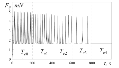
Figure 3: The time dependencies of the friction force $F_{ij}$ (31) at parameters of figure 2 and shear velocity $V_{ij}=17\cdot 10^{-12}$ m/s. Values of temperatures of friction surfaces are $T_{{\rm e}0}=50$ K, $T_{{\rm e}1}=230$ K, $T_{{\rm e}2}=400$ K, $T_{{\rm e}3}=490$ K, $T_{{\rm e}4}=550$ K.

It can be seen from the figure that at low temperatures of friction surfaces $T_{\rm e}=T_{{\rm e}0}$, the frequency of stick-slip transitions is large, and the dependence $F_{ij}(t)$ does not have the kinetic sections. This implies that the lubricant begins to solidify immediately after melting. With the increase in temperature ($T_{\rm e}=T_{{\rm e}1}$), both the frequency of peaks and their height become smaller. Frequency becomes smaller due to the appearance of kinetic sections, i.e., the lubricant now solidifies slower. A decrease in the height of peaks implies the decline of static friction force $F_{s}$ . With the further increase in $T_{\rm e}=T_{{\rm e}2}$, the kinetic section $F_{ij}=\rm const$ becomes more expressed, i.e., the lubricant exists during some time in the molten state at constant stresses which are already capable of supporting this state. However, due to dissipation the excess volume decreases and the lubricant solidifies, and the stick-slip mode is realized. At $T_{\rm e}=T_{{\rm e}3}$, the kinetic section becomes dominant, because most of the time the lubricant is in the liquid-like state. At $T_{\rm e}=T_{{\rm e}4}$, the lubricant melts ultimately and the kinetic mode is realized.

5 The effect of noise

The deterministic case is considered above, though, in some situations fluctuations critically effect the system [16, 17, 18]. We consider a case of fluctuations appearing due to inaccuracy of experiment where the value of the elastic strain is badly conserved in (25), and thus it fluctuates. To this end, in the right-hand part of (25) we add a stochastic source $\xi(t)$ (the white noise mathematically defined using the Wiener process [43]), which has moments

$$\langle\xi(t)\rangle=0,\qquad\langle\xi(t)\xi(t^{\prime})\rangle=2D\delta(t-t^{\prime}),$$ (35)

where $D$ is the intensity of source. With this addition, equation (25) has the form of Langevin equation:

$$\dot{\varepsilon}_{ij}^{\rm e}=-\frac{\varepsilon_{ij}^{\rm e}}{K(\gamma_{0}-\gamma_{1}f)}+\frac{V_{ij}}{h+\delta h}+\xi(t),$$ (36)

whose solution within the framework of Ito prezentation with account of (35) is carried out with the use of iteration procedure in the form [16, 18]:

$$\varepsilon_{ij(n+1)}^{e}=\varepsilon_{ij(n)}^{e}+\left(-\frac{\varepsilon_{ij}^{e}}{K(\gamma_{0}-\gamma_{1}f)}+\frac{V_{ij}}{h+\delta h}\right)\Delta t+\sqrt{2D\Delta t}W_{n}.$$ (37)

In order to model the random force $W_{n}$, the Box-Muller function is used [16, 18, 44]:

$$W_{n}=\sqrt{-2\ln r_{1}}\cos(2\pi r_{2}),\quad r_{i}\in(0,1],$$ (38)

where $r_{1}$ and $r_{2}$ are the pseudorandom numbers. The time dependencies of the friction force (31) at the parameters of figure 2 and using equation (37) are shown in figure 4.

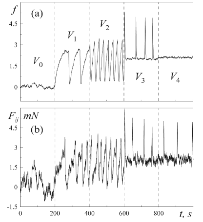
Figure 4: The time dependencies of friction force $F_{ij}$ (31) at parameters of figure 2 with consideration of noise: a: $D=2\cdot 10^{-9}$ s^-1; b: $D=8\cdot 10^{-8}$ s^-1.

In figure 4a, the intensity of noise is small and the deterministic modes are realized (cf. figure 2b). With the increase in intensity of fluctuations (figure 4b), the stochastic regime sets in at which the lubricant spontaneously solidifies and melts. The possibility of existence of such modes was shown by the methods of molecular dynamics [10].

6 Conclusions

The offered theory allows us to describe the effects observed at ultrathin lubricant film melting. Both the ordinary case of thermodynamic melting due to an increase in temperature and the shear melting due to disordering under the action of the applied external stresses are considered. It is shown that these two processes are interconnected and they cannot be examined separately. For example, at a high temperature of friction surfaces, the shear melting is realized at smaller stresses, and at a still greater increase in temperature, a lubricant melts even at zero stress (the thermodynamic melting is realized).

The stick-slip mode of friction, which is observed in experiments, is naturally considered in the model, and it is caused by the rapid relaxation of stress at reaching the liquid-like state by a lubricant. At the temperature of friction surfaces that does not provide the melting in a state of rest, the lubricant solidifies at such relaxation again and it is solid-like during the time that is necessary for the appearance of the stress at which melting occurs. Thus, the temperature effect and shear melting are taken into consideration. These are basic factors to be taken into account while carrying out the experiments. The obtained dependencies qualitatively coincide with the experimental ones.

Багатовимiрний термодинамiчний потенцiал для опису плавлення ультратонкої плiвки мастила мiж двома атомарно-гладкими поверхнями Л.С. Метловlabel1, О.В. Хоменкоlabel2, Я.О. Ляшенкоlabel2 label1 Донецький фiзико-технiчний iнститут iм. О.О. Галкiна НАН України, вул. Р. Люксембург, 72, 83114 Донецьк, Україна label2 Сумський державний унiверситет, вул. Римського-Корсакова, 2, 40007 Суми, Україна

References

- [1] Persson B.N.J., Sliding Friction. Physical Principles and Applications. Springer-Verlag, Berlin, 1998.
- [2] Yoshizawa H., Chen Y.-L., Israelachvili J., J. Phys. Chem., 1993, 97, 4128; \bibdoi10.1021/j100118a033; Yoshizawa H., Israelachvili J., J. Phys. Chem., 1993, 97, 11300; \bibdoi10.1021/j100145a031.
- [3] Smith E.D., Robbins M.O., Cieplak M., Phys. Rev. B, 1996, 54, 8252; \bibdoi10.1103/PhysRevB.54.8252.
-
[4]
Aranson I.S., Tsimring L.S., Vinokur V.M.,
Phys. Rev. B, 2002, 65, 125402;
\bibdoi10.1103/PhysRevB.65.125402. - [5] Popov V.L., Tech. Phys., 2001, 46, 605; \bibdoi10.1134/1.1372955.
- [6] Carlson J.M., Batista A.A., Phys. Rev. E, 1996, 53, 4153; \bibdoi10.1103/PhysRevE.53.4153.
-
[7]
Filippov A.E., Klafter J., Urbakh M.,
Phys. Rev. Lett., 2004, 92, 135503;
\bibdoi10.1103/PhysRevLett.92.135503. -
[8]
Tshiprut Z., Filippov A.E., Urbakh M.,
Phys. Rev. Lett., 2005, 95, 016101;
\bibdoi10.1103/PhysRevLett.95.016101. - [9] Khomenko A.V., Yushchenko O.V., Phys. Rev. E, 2003, 68, 036110; \bibdoi10.1103/PhysRevE.68.036110.
- [10] Braun O.M., Naumovets A.G., Surf. Sci. Rep., 2006, 60, 79; \bibdoi10.1016/j.surfrep.2005.10.004.
- [11] Khomenko A.V., Prodanov N.V., Condens. Matter Phys., 2008, 11, 615.
- [12] Khomenko A.V., Prodanov N.V., Carbon, 2010, 48, 1234; \bibdoi10.1016/j.carbon.2009.11.046.
- [13] Prodanov N.V., Khomenko A.V., Surface Science, 2010, 604, 730; \bibdoi10.1016/j.susc.2010.01.024.
- [14] Khomenko A.V., Lyashenko I.A., J. Phys. Stud., 2007, 11, 268 (in Ukrainian).
-
[15]
Horn R.G., Smith D.T., Haller W.,
Chem. Phys. Lett., 1989, 162, 404;
\bibdoi10.1016/0009-2614(89)87066-6. - [16] Khomenko A.V., Lyashenko I.A., Tech. Phys., 2007, 52, 1239; \bibdoi10.1134/S1063784207090241.
- [17] Khomenko A.V., Lyashenko I.A., Tech. Phys., 2010, 55, 26; \bibdoi10.1134/S1063784210010056.
- [18] Khomenko A.V., Lyashenko I.A., Borisyuk V.N., FNL, 2010, 9, 19; \bibdoi10.1142/S0219477510000046.
- [19] Khomenko A.V., Lyashenko I.A., FNL, 2007, 7, L111; \bibdoi10.1142/S0219477507003763.
- [20] Demirel A.L., Granick S., J. Chem. Phys., 1998, 109, 6889; \bibdoi10.1063/1.477256.
- [21] Reiter G. et al., J. Chem. Phys., 1994, 101, 2606; \bibdoi10.1063/1.467633.
- [22] Israelachvili J., Surf. Sci. Rep., 1992, 14, 109; \bibdoi10.1016/0167-5729(92)90015-4.
- [23] Khomenko A.V., Lyashenko I.A., Phys. Sol. State, 2007, 49, 936; \bibdoi10.1134/S1063783407050228.
- [24] Khomenko A.V., Lyashenko I.A., Phys. Lett. A, 2007, 366, 165; \bibdoi10.1016/j.physleta.2007.02.010.
- [25] Landau L.D., Lifshitz E.M., Course of Theoretical Physics, Vol.5: Statistical Physics, 4th ed.. Butterworth, London, 1999.
-
[26]
Metlov L.S.,
Bulletin of Russian Academy of Sciences, Physics 2008, 72,
1283;
\bibdoi10.3103/S1062873808090311. - [27] Glezer A.M., Metlov L.S., Phys. Sol. State, 2010, 52, 1090; \bibdoi10.1134/S1063783410060089.
- [28] Metlov L.S., Bulletin of Donetsk Univ., 2007, 2, 108 (in Russian).
- [29] Metlov L.S. Preprint arXiv:cond-mat/0711.0399, 2007.
- [30] Metlov L.S. Preprint arXiv:cond-mat.mess-hall/0910.5503, 2009.
- [31] Metlov L.S. Preprint arXiv:physics.comp-ph/0912.2085, 2009.
- [32] Metlov L.S. Preprint arXiv:cond-mat.stat-mech/1003.0450, 2010.
-
[33]
Thompson P.A., Grest G.S., Robbins M.O.,
Phys. Rev. Lett., 1992, 68, 3448;
\bibdoi10.1103/PhysRevLett.68.3448. - [34] Gee M.L., McGuiggan P.M., Israelachvili J.N., J. Chem. Phys., 1990, 93, 1895; \bibdoi10.1063/1.459067.
- [35] Li H., Theory of phase transitions in disordered crystal solids. Ph.D. Thesis, Georgia Institute of Technology, 2009.
- [36] Kachanov L.M., Basics of Theory of Plasticity. Nauka, Moscow, 1969 (in Russian).
- [37] Vonsovskii S.V., Magnetism. John Wiley, New York, 1974.
-
[38]
Kut’in E.I., Lorman V.L., Pavlov S.V.,
Sov. Phys. Uspekhi, 1991, 34, 497;
\bibdoi10.1070/PU1991v034n06ABEH002385. -
[39]
Gouyet J-.F., Plapp M., Dieterich W., Maass P.,
Adv. Phys., 2003, 52, 523;
\bibdoi10.1080/00018730310001615932. - [40] Panin V.E., Yegorushkin V.E., Khon Yu.A., Elsukova T.F., Izvestiya VUZov, Physics, 1982, 12, 5 (in Russian); \bibdoi10.1007/BF00900288.
- [41] Landau L.D., Lifshitz E.M., Course of Theoretical Physics, vol.7: Theory of Elasticity, 3rd ed.. Pergamon Press, New York, 1986.
- [42] Luengo G., Israelachvili J., Granick S., Wear, 1996, 200, 328; \bibdoi10.1016/S0043-1648(96)07248-1.
- [43] Gardiner C.W., Handbook of Stochastic Methods. Springer, Berlin, 1983.
- [44] Press W.H. et al., Numerical Recipes in C: the Art of Scientific Computing. Cambridge University Press, New York, 1992.