A theoretical scheme of thermal-light ghost imaging by $N$th-order intensity correlation

Abstract

In this paper, we propose a theoretical scheme of ghost imaging in terms of $N$th-order correlated thermal light. We obtain the Gaussian thin lens equations in the ghost imaging protocol. We show that it is possible to produce $N-1$ ghost images of an object at different places in a nonlocal fashion by means of a higher-order correlated imaging process with an $N$th-order correlated thermal source and correlation measurement. We investigate the visibility of the ghost images in the scheme, and obtain the upper bounds of the visibility for the $N$th-order correlated thermal-light ghost imaging. It is found that the visibility of the ghost images can be dramatically enhanced when the order of correlation becomes larger.

I Introduction

Ghost imaging with thermal light ben ; gat1 ; gat2 ; gat3 ; che ; ca ; cli ; bra ; val ; fer ; zh ; mey ; er ; gat4 ; bac ; cai ; zha ; scar ; dan ; liu ; zhan has been studied extensively in recent years. Bennink and coworkers ben first pointed out that ghost imaging can also be realized using a classical source with the appropriate correlations. A thermal or quasi-thermal source can exhibit such a classical correlation. A very close formal analogy was demonstrated between ghost imaging with thermal and quantum-entangled beams in Refs. gat2 ; gat3 ; che ; ca , which implied that classically correlated beams were able to emulate the relevant features of quantum ghost imaging. Number of experiments on thermal light ghost imaging have been performed in Refs. val ; fer ; zh ; mey ; zhan . A unified treatment of classical and quantum ghost imaging was established in terms of Gaussian-state analysis in Ref. er .

Recently, some attention has been paid to the physics of thermal-light ghost imaging mey ; shi ; erk ; ga ; sca ; wa ; bre ; sh ; sha and higher-order-coherence or correlation effects of thermal light ou ; ba ; li ; dz ; aga ; ric . The higher-order coherence or correlation has shown attractive properties in practical applications. Multiphoton imaging with thermal light is one of these exciting areas. In a previous work, our group theoretically initiated a study of thermal-light ghost imaging in terms of higher-order correlated thermal light ou . We proposed a thermal-light ghost imaging scheme with third-order correlated thermal light. In this scheme, a third-order correlated thermal-light source, a test optical arm and two reference optical arms are used to produce two ghost images. Two ghost images are created at two different places in a nonlocal fashion as a consequence of the third order correlation of the involved optical fields. It was shown that the third-order correlated imaging includes richer correlated imaging effects than the second-order correlated one. In this paper, we want to propose a thermal-light ghost imaging scheme with $N$th-order intensity correlation and investigate the visibility of the ghost images. We show that the usual second- and third-order ghost imaging are only two particular examples of our present scheme.

The paper is organized as follows. In Sec. II, begin with the thermal-light source with $N$th-order correlation, we will propose the thermal-light ghost imaging scheme with $N$th-order intensity correlation. In Sec. III, the visibility of the ghost images in the proposed scheme will be investigated. Finally, we shall conclude our paper with discussions and remarks in the last section.

II Ghost imaging scheme with $N$-order correlated thermal light

The basic setup for ghost imaging with $N$-order correlated thermal light is indicated in Figure 1 which includes one test optical arm and $N-1$ reference optical arms. First arm is the test arm. An unknown object with transmission function $T(x)$ and a collective lens with focal length $f_{c}$ are placed on the test arm while there is one imaging lens with focal lengths $f_{i}$ on each reference arm. The object is placed at the focal plane of the collective lens at distance $z_{1}$ from the thermal-light source. The distance between $i$th imaging lens and the thermal-light source is $z_{i0}$ with $i=2,3,\cdots,N$. The first detector $\tt{D_{1}}$ is a bucket detector placed at the focal plane of the collective lens on the right-hand side. The other detectors are scanning detectors $\tt{D_{i}}$ with $i=2,3,\cdots,N$ which are placed at distances $z_{i1}$ from $i$th imaging lens. The signals from the $N$ photon counting detectors are sent to an electronic coincidence circuit to measure the rate of coincidence counts.

The thermal light source with $N$th-order intensity correlation, usually obtained by illuminating a laser beam into a slowly rotating ground glass, is divided into $N$ beams, which can be implemented by an appropriate combination of $N-1$ beam splitters. Consider a monochromatic plane wave described by the field $E_{0}\exp[i(k_{0}z-w_{0}t)]$ illuminating a material containing disordered scattering centers. After scattering, the field can be written as $E(x,z,t)=\int E(\mathbf{q})\exp[i(q\cdot x+k_{z}z-w_{0}t)]d\mathbf{q}$ where $\mathbf{q}$ is the transverse wave vector introduced by the random scattering and satisfies the relation $|\mathbf{q}|^{2}+k_{z}^{2}=k_{0}^{2}$. Hence, $E(\mathbf{q})$ is a stochastic variable obeying Gaussian statistics. However, the scattered waves with different transverse wave vectors are statistically independent. If $|\mathbf{q}|\ll k_{0}$, the scattered field can be approximately written as $E(x,z,t)=A(x)\exp[(i(k_{0}z-w_{0}t)]$ where $A(x)=\int E(\mathbf{q})\exp[i(\mathbf{q}\cdot\mathbf{x})]d\mathbf{q}$ is the slowly varying envelope. As a result, we have defined a monochromatic thermal light random in both strength and propagation direction. According to the Wiener-Khintchine theorem, the first-order spectral correlation satisfies the following expression

$$\langle E^{\ast}(\mathbf{q})E(\mathbf{q^{\prime}})\rangle=S(\mathbf{q})\delta(\mathbf{q}-\mathbf{q^{\prime}}),$$ (1)

where $S(\mathbf{q})$ is the power spectrum of the spatial frequency. For any field with thermal statistics, all high-order correlations can be expressed in terms of the first-order ones due to $\langle E(\mathbf{q})\rangle=0$ man . Then, $N$th-order spectral correlation of thermal light can be written as

$$\left\langle\prod^{N}_{i=1}E^{\ast}(\mathbf{q}_{i})E(\mathbf{q}_{i}^{\prime})\right\rangle = \sum_{\begin{array}[]{c}r_{i}\neq r_{j}\\ s_{i}\neq s_{j}\end{array}}^{N}\left(\prod^{4}_{i=1}\delta(\mathbf{q}_{r_{i}}-\mathbf{q}_{s_{i}}^{\prime})\right)^{\prime}$$ (5)

$$\times S(\mathbf{q}_{1})S(\mathbf{q}_{2})\cdots S(\mathbf{q}_{N}),$$

where the prime in the summation means that all of repeating terms are subtracted from the summation over $r_{i}$ and $r_{j}$. After passing through a combination of $N-1$ beam splitters, the thermal light with $N$th-order spectral correlation is divided into $N$ correlated thermal-light beams which are input light beams of the test and reference arms. For simplicity, we consider the one-dimensional case, and let $x_{0}$ and $x_{n}$ with $n=1,2,\cdots,N$ be the transverse coordinates of the source plane and detection planes, respectively. Here we have assumed that the starting planes of the $N$ thermal-light beams are overlapped. Let $H_{1}(x_{1},x_{0})$ be the impulse response function of the test arm, and $H_{n}(x_{n},x_{0})$ with $n=2,3,\cdots,N$ be the impulse response function of $n$th reference arm, respectively. Assume that the light field on the $n$th detection planes is denoted as $E(x_{n})$, which is connected with the optical field of the thermal-light source through the following relation

$$E\left(x_{n}\right)=\int h_{n}\left(x_{n},-q_{n}\right)E\left(q_{n}\right)dq_{n}$$ (6)

where $h_{n}(x_{n},q_{n})=(1/\sqrt{2\pi})\int H_{n}(x_{n},x_{0})\exp(-iq_{n}x_{0})dx_{0}$ is the Fourier transformation of the impulse response function $H_{n}(x_{n},x_{0})$. Then, the $N$th-order correlation function of the joint intensity at the $N$ detection planes can be expressed as

$$G^{\left(N\right)}\left(x_{1},x_{2},\cdots,x_{N}\right)=\left\langle\prod^{N}_{i=1}E^{\ast}\left(x_{i}\right)E\left(x_{i}^{\prime}\right)\right\rangle.$$ (7)

The rate of coincidence counts is governed by the $N$th-order correlation function given by equation (7) which can be calculated in terms of the impulse response functions of the relevant optical systems. The impulse response functions Cao in the reference arms can be written as

$$h_{r}(x_{r},q) = \sqrt{\frac{f_{r}}{2\pi\left(f_{r}-z_{r1}\right)}}e^{i\varphi_{r}(x_{r},q)},$$ (8)

$$\varphi_{r}(x_{r},q) = k\left(z_{r0}+z_{r1}\right)-\frac{q^{2}}{2k}\left(z_{r0}+\frac{z_{r1}f_{r}}{f_{r}-z_{r1}}\right)$$ (9)

$$-\frac{(2qf_{r}+kx_{r})x_{r}}{2(f_{r}-z_{r1})},$$

where $z_{r1}\neq f_{r}$ with $r=2,3,\cdots,N$, and the impulse response function in the test arm is given by

$$h_{1}(x_{1},q) = \frac{1}{2\pi}\sqrt{\frac{k}{if_{c}}}\exp\left[ik\left(z_{1}+2f_{c}\right)+\left(-i\frac{z_{1}q^{2}}{2k}\right)\right]$$ (10)

$$\times\int T\left(x\right)\exp\left[-i\left(\frac{kx_{1}}{f_{c}}+q\right)x\right]dx.$$

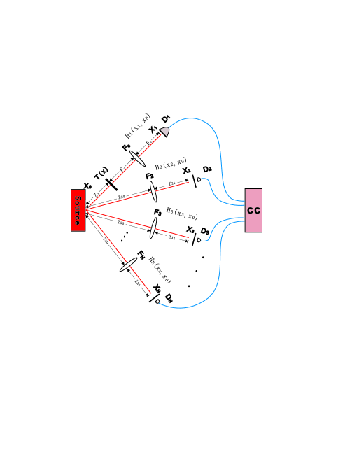
Figure 1: (Color online) Schematic of the setup for implementing ghost imaging with $N$th-order correlated thermal light. It consists of one test arm and $N-1$ reference arms. The test arm includes the object $T(x)$, the collection lens $\tt{F_{c}}$, and the bucket detector $\tt{D_{1}}$. The object and the detector are placed in its two focal planes of the collection lens, respectively. Each reference arm includes one imaging lens and a scanning detector denoted by $\tt{F_{i}}$ and $\tt{D_{i}}$ with $i=2,3,\cdots,N-1$, respectively.

In order to obtain the $N$th-order correlation function given by equation (4), we first calculate the following integrations:

$$I_{r} = \int S\left(q\right)\left|h_{r}\left(x_{r},-q\right)\right|^{2}dq,$$ (11)

$$C_{rr^{\prime}} = \int S\left(q\right)h_{r}^{\ast}\left(x_{r},-q\right)h_{r^{\prime}}\left(x_{r^{\prime}},-q\right)dq,$$ (12)

where both $r$ and $r^{\prime}$ may take $1,2,\cdots,N$, but $r\neq r^{\prime}$. In the broadband limit, S(q) can be regarded as a constant S(0). Hence we have the total intensity of the thermal light $S_{0}=\int S(q)dq\approx S(0)q_{0}$, where $q_{0}$ is the spectral bandwidth of the source. Substituting the impulse response functions of the test and reference arms given by equations (8) and (10) into equations (11) and (12), we obtain

$$I_{1} = \frac{S(0)k}{4\pi^{2}f_{c}}\int\left|T\left(x\right)\right|^{2}dx,\hskip 8.5359ptI_{r}=\frac{f_{r}S(0)q_{0}}{2\pi\left(f_{r}-z_{r1}\right)},$$ (13)

$$C_{r1} = \frac{S(0)}{2\pi}\sqrt{\frac{kf_{r}}{i2\pi f_{c}\left(f_{r}-z_{r1}\right)}}\int T(x)e^{i\phi_{r1}(x,q)}dxdq,$$

$$C_{rr^{\prime}} = \frac{S(0)}{2\pi}\sqrt{\frac{f_{r}f_{r^{\prime}}}{\left(f_{r}-z_{r1}\right)\left(f_{r^{\prime}}-z_{r^{\prime}1}\right)}}\int e^{i\phi_{rr^{\prime}}(q)}dq,$$

where both $r$ and $r^{\prime}$ may take $2,3,\cdots,N$ but $r\neq r^{\prime}$, and we have introduced two phase functions

$$\phi_{r1}(x,q) = \frac{q^{2}}{2k}\left(z_{r0}-z_{1}+\frac{z_{r1}f_{r}}{f_{r}-z_{r1}}\right)-\left(q+\frac{kx_{1}}{f_{c}}\right)x$$ (16)

$$+qX_{r}-k(z_{r0}+z_{r1}-z_{1}-2f_{c}),$$

$$\phi_{rr^{\prime}}(q) = \frac{kx^{2}_{r}}{2\left(f_{r}-z_{r1}\right)}-\frac{kx^{2}_{r^{\prime}}}{2\left(f_{r^{\prime}}-z_{r^{\prime}1}\right)}$$

$$-\frac{q^{2}}{2k}\left(z_{r^{\prime}0}-z_{r0}+\frac{z_{r^{\prime}1}f_{r}^{\prime}}{f_{r}^{\prime}-z_{r^{\prime}1}}-\frac{z_{r1}f_{r}}{f_{r}-z_{r1}}\right)$$

$$-q\left(X_{r^{\prime}}-X_{r}\right)+k(z_{r^{\prime}0}+z_{r^{\prime}1}-z_{r0}-z_{r1}),$$

where the scaled positions $X_{r}=f_{r}x_{r}/(f_{r}-z_{r1})$.

From equations (11) and (13), it is straightforward to see that when the positions of the object, ghost images, and the lenses obey the following Gaussian thin lens equations for the $N$th-order correlated imaging

$$\frac{1}{z_{r0}-z_{1}}+\frac{1}{z_{r1}}=\frac{1}{f_{r}}\text{ \ \ \ \ \ \ }(r=2,3,\cdots,N),$$ (18)

the cross-correlation functions of intensity fluctuation can be simplified as

$$C_{r1} = \frac{S(0)}{2\pi}\sqrt{\frac{kf_{r}}{i2\pi f_{c}\left(f_{r}-z_{r1}\right)}}\exp\left(-\frac{ikx_{1}X_{r}}{f_{c}}\right)T(X_{r}),$$

$$C_{rr^{\prime}} = \frac{S(0)}{2\pi}\sqrt{\frac{f_{r}f_{r^{\prime}}}{\left(f_{r}-z_{r1}\right)\left(f_{r^{\prime}}-z_{r^{\prime}1}\right)}}e^{i\phi_{rr^{\prime}}(0)}\delta(X_{r^{\prime}}-X_{r}).$$

When Gaussian thin lens equations are satisfied, and $X_{2}\neq X_{3}\cdots\neq X_{N}$ the $N$th-order correlation function of the joint intensity at the $N$ detection planes given by equation (7) can be reduced to the following form

$$G^{\left(N\right)}\left(x_{1},x_{2},\cdots,x_{N}\right)$$

$$=\sum^{N}_{r_{i}\neq r_{j}=2}\left(I_{r_{1}}I_{r_{2}}\cdots I_{r_{N-2}}|C_{r_{N-1}1}|^{2}\right)^{\prime}+I_{1}I_{2}\cdots I_{N},$$

where the prime on the right-hand side of above equation means that repeating terms in the summation over $r_{i}$ and $r_{j}$ should be subtracted. The last term on the right-hand equation (18) is the background term which is the multiplication of the intensity distribution at the $N$ detectors. It does not contribute to the correlated imaging, but it may affect the visibility of produced ghost images. Each term in the summation over $r_{i}$ and $r_{j}$ is the multiplication of the intensity distribution at detector $\tt{D_{i}}$ and the intensity fluctuation correlation between $\tt{D_{1}}$ and $\tt{D_{i}}$ with $i=2,3,\cdots,N$, which gives the information of the object imaged at $\tt{D_{i}}$.

In particular, when the $N-1$ reference arms are identic, i.e., $f_{2}=f_{3}=\cdots=f_{N}$, $z_{20}=z_{30}=\cdots=z_{N0}$ and $z_{21}=z_{31}=\cdots=z_{N1}$, we have $I_{2}=I_{3}=\cdots=I_{N}\equiv I$, $N$th-order correlation function becomes

$$G^{(N)}=I^{N-1}I_{1}+\chi I^{N-2}\sum^{N}_{i=2}|T(X_{i})|^{2},$$ (22)

where we have introduced the parameter $\chi=S^{2}(0)kf_{r}/[8\pi^{3}f_{c}\left(f_{r}-z_{r1}\right)]$.

Equation (19) indicates that for the object placed at the test arm, $N-1$ ghost images can be produced in the $N-1$ reference arms through coincidence count measurements upon $N$ detectors. Each ghost image is an amplified image of the object with the amplifying rate $f_{r}/(f_{r}-z_{r1})$ with $r=2,3,\cdots,N$ since $X_{r}=f_{r}x_{r}/(f_{r}-z_{r1})$. From the Gaussian thin lens equations of $N$th-order correlated imaging given by equation (15) we can see that the higher-order correlated imaging exhibits richer imaging effects. In fact, the imaging equation (15) indicates that $z_{r0}-z_{1}$ is the object distance while $z_{r1}$ is the image distance for $r$th joint path with $r=2,3,\cdots,N$. Just as the ordinary imaging law, when the object distance of the $r$th joint path $z_{r0}-z_{1}$ is greater (less) than the focal length $f_{r}$, the correlated image is real (virtual). As a specific example, we consider the case of $N=4$. In this case, from the imaging equation (15) we can obtain the following eight ghost-image configurations: (1) when $z_{r0}-z_{1}>f_{r}$ with $r=2,3,$ and $4$, the three ghost images are real; (2) when $z_{r0}-z_{1}<f_{r}$ with $r=2,3,$ and $4$, the three ghost images are virtual; (3) when $z_{20}-z_{1}>f_{2}$, $z_{30}-z_{1}<f_{3}$ and $z_{40}-z_{1}<f_{4}$, one ghost image is real at the position $x_{2}$, the other two ghost images are virtual at the positions $x_{3}$ and $x_{4}$; (4) when $z_{30}-z_{1}>f_{3}$, $z_{20}-z_{1}<f_{2}$ and $z_{40}-z_{1}<f_{4}$, the ghost image at the position $x_{3}$, two ghost images at the positions $x_{2}$ and $x_{4}$ are virtual; (5) when $z_{40}-z_{1}>f_{4}$, $z_{20}-z_{1}<f_{2}$ and $z_{30}-z_{1}<f_{3}$, the ghost image at the position $x_{4}$ is real, two ghost images at the positions $x_{2}$ and $x_{3}$ are virtual; (6) when $z_{20}-z_{1}>f_{2}$, $z_{30}-z_{1}<f_{3}$ and $z_{40}-z_{1}<f_{4}$, two ghost images at the positions $x_{2}$ and $x_{3}$ are real, the ghost image at the position $x_{4}$ is virtual; (7) when $z_{20}-z_{1}>f_{2}$, $z_{40}-z_{1}<f_{4}$ and $z_{30}-z_{1}<f_{3}$, two ghost images at the positions $x_{2}$ and $x_{4}$ are real, the ghost image at the position $x_{3}$ is virtual; (8) when $z_{30}-z_{1}>f_{3}$, $z_{40}-z_{1}<f_{4}$ and $z_{20}-z_{1}<f_{2}$, two ghost images at the positions $x_{3}$ and $x_{4}$ are real, the ghost image at the position $x_{2}$ is virtual.

It is obvious that when $N=2,3$, the usual results of the second- and third-order thermal-light ghost imaging are recovered.

III Visibility of ghost images

The visibility is an important parameter to estimate the quality of a ghost image. We first generalize the visibility of the second-order correlated imaging Bache ; gat4 to the case of $N$th-order correlated imaging as follows

$$V^{\left(N\right)}=\frac{\left[G^{\left(N\right)}-\prod^{N}_{i=1}\langle I_{i}\rangle\right]_{\max}}{\left[G^{\left(N\right)}\right]_{\max}}.$$ (23)

For our present scheme of the $N$th order thermal-light imaging, substituting equations (19) into equation (20), we obtain the visibility

$$V^{\left(N\right)}=\frac{\left[\sum^{N}_{i=2}|T(X_{i})|^{2}\right]_{\max}}{\left[q_{0}\int\left|T\left(x\right)\right|^{2}dx+\sum^{N}_{i=2}|T(X_{i})|^{2}\right]_{\max}},$$ (24)

which indicates that the visibility depends on not only the spectral bandwidth of the thermal-light source $q_{0}$ and the transmission function $T(x)$ but also the order number of the correlation of the thermal-light source. The visibility can be enhanced with the decrease of the spectral bandwidth. An increase of the transmission leads to a decrease of the visibility since when the transmission area increases, more points contribute to the background that directly makes the visibility decrease.

In order to see the relationship between the visibility and the order number of the correlation, making use of equations (10) and (11), we have

$$\frac{\left\langle I_{1}\right\rangle\left\langle I_{r}\right\rangle}{\left|\left\langle E^{*}(x_{1})E(x_{r})\right\rangle\right|^{2}}=q_{0}\int\left|T\left(x\right)\right|^{2}dx,$$ (25)

where $r=2,3,\cdots,N$. According to the Cauchy-Schwartz inequality $\left\langle I_{1}\right\rangle\left\langle I_{r}\right\rangle\geq\left|\left\langle E^{\ast}\left(x_{1}\right)E\left(x_{r}\right)\right\rangle\right|^{2}$, which means that $q_{0}\int\left|T\left(x\right)\right|^{2}dx\geq 1$. Hence, we find that

$$V^{\left(N\right)}\leq\frac{\left[\sum^{N}_{i=2}|T(X_{i})|^{2}\right]_{\max}}{\left[1+\sum^{N}_{i=2}|T(X_{i})|^{2}\right]_{\max}}\leq\frac{N-1}{N},$$ (26)

which implies that the visibility of the ghost images can be dramatically enhanced when the order of correlation becomes larger. For $N$th order correlated thermal-light imaging, the upper bounds of the visibility is given by $V^{(N)}_{b}=(N-1)/N$. As expected, when $N=2$ the upper bound of the visibility of the second correlated imaging gat4 is $1/2$.

IV Concluding remarks

In conclusion, we have proposed a theoretical scheme of ghost imaging in terms of $N$th-order correlated thermal light. Our scheme includes one test arm and $N-1$ references arms. One object is placed on the test arm. $N-1$ ghost images are produced in the reference arms in a nonlocal fashion by means of a higher-order correlated imaging process with an $N$th-order correlated thermal source and correlation measurements. We have derived the Gaussian thin lens equations which the positions of the ghost images obey in the ghost imaging protocol. We have also investigated the visibility of the ghost images in the scheme, and obtained the upper bounds of the visibility for the $N$th-order correlated thermal-light ghost imaging. It has been shown that the visibility depends on not only the spectral bandwidth of the thermal-light source and the transmission area of the object but also the order number of the correlation of the thermal-light source. It is found that the visibility of the ghost imagines can be dramatically enhanced when the order of correlation becomes larger. Our present scheme is a many-ghost imaging protocol. On one hand, it gives rise to a theoretical origin for developing many-ghost imaging technology. This gives rise to the possibility of experimentally producing correlated many ghost images. In fact, the higher-order correlated imaging opens up new avenues for realizing multi-port information processing. On the other hand, physically these ghost images stem from higher-order coherence or correlation of optical fields. In this sense, the appearance of the many ghost images reveals an observable physical effect of higher-order coherence or correlation of optical fields. Hence, it is of very significance to study higher-order correlated imaging not only for well understanding the essential physics behind the higher coherence or correlation of optical fields but also for developing multi-port information processing technology. The experimental realization for the many ghost imaging protocol proposed here and practical applications of the many ghost imaging phenomenon deserves further investigation.

- (1) R. S. Bennink, S. J. Bentley, and R. W. Boyd, Phys. Rev. Lett. 89, 113601 (2002).
- (2) A. Gatti, E. Brambilla, and L. A. Lugiato, Phys. Rev. Lett. 90,133603 (2003).
- (3) A. Gatti, E. Brambilla, M. Bache, and L. A. Lugiato, Phys. Rev. Lett. 93, 093602 (2004).
- (4) A. Gatti, E. Brambilla, M. Bache, and L. A. Lugiato, Phys. Rev. A 70, 013802 (2004).
- (5) J. Cheng and S. S. Han, Phys. Rev. Lett. 92, 093903 (2004).
- (6) Y. Cai and S. Y. Zhu, Opt. Lett. 29, 2716 (2004).
- (7) K. W. C. Chan, M. N. O’Sullivan, and R. W. Boyd, Phys. Rev. A 79, 033808 (2009).
- (8) E. Brambilla, A. Gatti, M. Bache, and L. A. Lugiato, Fortschr. Phys. 52, 1080 (2004).
- (9) A. Valencia, G. Scarcelli, M. D’Angelo, and Y. H. Shih, Phys. Rev. Lett. 94, 063601 (2005).
- (10) F. Ferri, D. Magatti, A. Gatti, M. Bache, E. Brambilla, and L. A. Lugiato, Phys. Rev. Lett. 94, 183602 (2005).
- (11) D. Zhang, Y. H. Zhai, L. A. Wu, and X. H. Chen, Opt. Lett. 30, 2354 (2005).
- (12) R. Meyers, K. S. Deacon, and Y. H. Shih, Phys, Rev. A 77, 041801 (2008).
- (13) B. I. Erkmen and J. H. Shapiro, Phys. Rev. A 77, 043809 (2008); ibid. 79, 023833.
- (14) A. Gatti, M.Bache, D. Magatti, E. Brambilla, F. Ferri, and L. A. Lugiato, J. Mod. Opt. 53, 739 (2006).
- (15) M. Bache, D. Magatti, F. Ferri, A. Gatti, E. Brambilla, and L. A. Lugiato, Phys. Rev. A 73, 053802 (2006).
- (16) Y. Cai and S. Y. Zhu, Phys. Rev. E 71, 056607 (2005).
- (17) Y. H. Zhai, X. H. Chen, D. Zhang, and L. A. Wu, Phys. Rev. A 72, 043805 (2005).
- (18) G. Scarcelli, V. Berardi, and Y. H. Shih, Phys. Rev. Lett. 96, 063602 (2006).
- (19) M. D’Angelo, Y. H. Kim, S. P. Kulik, and Y. H. Shih, Phys. Rev. Lett. 92, 233601 (2004).
- (20) H. Liu, X. Shen, D. M. Zhu, and S. Han, Phys. Rev. A 76, 053808 (2007).
- (21) M. Zhang, Q. Wei, X. Shen, Y. Liu, H. Liu, J. Cheng, and S. Han, Phys. Rev. A 75, 021803 (2007).
- (22) G. Scarcelli, V. Berardi, and Y. H. Shih, Appl. Phys. Lett. 88, 061106 (2006).
- (23) Y. H. Shih, e-print arXiv:0805.1166.
- (24) B. I. Erkmen and J. H. Shapiro, Phys. Rev. A 78, 023835 (2008).
- (25) A. Gatti, M. Bondani, L. A. Lugiato, M. G. A. Paris, and C. Fabre, Phys. Rev. Lett. 98, 039301 (2007).
- (26) L. G. Wang, S. Qamar, S. Y. Zhu, and M. S. Zubairy, Phys. Rev. A 79, 033835 (2009).
- (27) M. E. Brezinski and B. Liu, Phys. Rev. A 78 063824 (2008).
- (28) Y. H. Shih, Front. Phys. China, 2, 125 (2007).
- (29) J. H. Shapiro, Phys. Rev. A 78, 061802(R) (2008).
- (30) L. H. Ou and L. M. Kuang, J. Phys. B 40, 1833 (2007).
- (31) Y. F. Bai and S. S. Han, Phys. Rev. A 76, 043828 (2007).
- (32) J. B. Liu and Y. H. Shih, Phys. Rev. A 79, 023819 (2009).
- (33) D. Z. Cao, J. Xiong, S. H. Zhang, L. F. Lin, L. Gao, and K. G. Wang, Appl. Phys. Lett. 92, 201102 (2008).
- (34) I. N. Agafonov, M. V. Chekhova, T. Sh. Iskhakov, and A. N. Penin, Phys. Rev. A 77 053801 (2008).
- (35) Th. Richter, Phys. Rev. A 42, 1817 (1990).
- (36) L. Mandel and L. Wolf, Optical Coherence and Quantum Optics (Cambridge University Press, Cambridge, 1995) p428.
- (37) D. Z. Cao, J. Xiong, and K. G. Wang, Phys. Rev. A 71, 013801 (2005); D. Z. Cao and K. G. Wang, Phys. Lett. A 333, 23 (2004).
- (38) M. Bache, D. Magatti, F. Ferri, A. Gatti, E. Brambilla, and L. A. Lugiato, Phys. Rev. A 73, 053802 (2006).