CMB polarization features from inflation versus reionization
Abstract
The angular power spectrum of the cosmic microwave background temperature anisotropy observed by WMAP has an anomalous dip at and bump at . One explanation for this structure is the presence of features in the primordial curvature power spectrum, possibly caused by a step in the inflationary potential. The detection of these features is only marginally significant from temperature data alone. However, the inflationary feature hypothesis predicts a specific shape for the -mode polarization power spectrum with a structure similar to that observed in temperature at . Measurement of the CMB polarization on few-degree scales can therefore be used as a consistency check of the hypothesis. The Planck satellite has the statistical sensitivity to confirm or rule out the model that best fits the temperature features with significance, assuming all other parameters are known. With a cosmic variance limited experiment, this significance improves to . For tests of inflationary models that can explain both the dip and bump in temperature, the primary source of uncertainty is confusion with polarization features created by a complex reionization history, which at most reduces the significance to for Planck and for an ideal experiment. Smoothing of the polarization spectrum by a large tensor component only slightly reduces the ability of polarization to test for inflationary features, as does requiring that polarization is consistent with the observed temperature spectrum given the expected low level of correlation on few-degree scales. If polarized foregrounds can be adequately subtracted, Planck will supply valuable evidence for or against features in the primordial power spectrum. A future high-sensitivity polarization satellite would enable a decisive test of the feature hypothesis and provide complementary information about the shape of a possible step in the inflationary potential.
I Introduction
Our best constraints on the shape of the primordial power spectrum at large scales come from observations of the cosmic microwave background (CMB) anisotropy by the Wilkinson Microwave Anisotropy Probe (WMAP) Bennett et al. (2003); Hinshaw et al. (2009). The latest (5-year) WMAP data Nolta et al. (2009); Dunkley et al. (2009) continue to be well described by the simplest inflationary scenario of a single, slowly rolling, minimally coupled scalar field with a canonical kinetic term Komatsu et al. (2009); Peiris and Easther (2008); Kinney et al. (2008); Alabidi and Lidsey (2008); Lesgourgues and Valkenburg (2007). Since the 3-year release Spergel et al. (2007), the WMAP data have indicated a deviation from scale invariance — a red tilt of the scalar spectral index — the significance of which has been debated in the literature from a Bayesian model selection point of view (e.g. Parkinson et al. (2006); Gordon and Trotta (2007)). Recent minimally-parametric reconstructions of the primordial power spectrum incorporating some form of penalty for “unnecessary” complexity Verde and Peiris (2008); Bridges et al. (2008) show some evidence for a red tilt, but no evidence for scale dependence of the spectral index. These methods, as currently implemented, are not very sensitive to sharp, localized features in the primordial power spectrum.
However, it has been pointed out ever since the original data release Spergel et al. (2003); Peiris et al. (2003) that there are several sharp glitches in the WMAP temperature () power spectrum. In particular, several model-independent reconstruction techniques that are sensitive to features localized in a narrow wavenumber range have consistently picked out a feature at that leads to an improvement of over a smooth power-law spectrum Hannestad (2004); Shafieloo and Souradeep (2004); Mukherjee and Wang (2003); Shafieloo et al. (2007); Nicholson and Contaldi (2009).
Power spectrum features could arise, in principle, in more general classes of inflationary models where slow roll is momentarily violated. Such an effect can be phenomenologically modeled as a discontinuity or singularity in the inflaton potential Starobinsky (1992); Adams et al. (2001); Joy et al. (2008a). A “step-like” feature Adams et al. (2001), in particular, would be a good effective field theory description of a symmetry breaking phase transition in a field coupled to the inflaton in multi-field models Silk and Turner (1987); Holman et al. (1991); Polarski and Starobinsky (1992); Adams et al. (1997); Hunt and Sarkar (2004), which can arise in supergravity Lesgourgues (2000) or M-theory-inspired Burgess et al. (2005); Ashoorioon and Krause (2006) contexts. Several analyses have confronted such phenomenological descriptions of features in the inflationary potential with current data Peiris et al. (2003); Covi et al. (2006); Hamann et al. (2007); Hunt and Sarkar (2007); Joy et al. (2008b); Martin and Ringeval (2004); Kawasaki et al. (2005); Jain et al. (2009).
It is debatable whether the large scale feature seen in the WMAP spectrum is a signal of exotic primordial physics or merely a statistical anomaly. Currently, our information about the smoothness of the primordial power spectrum is dominated by the temperature data. However, future high fidelity CMB polarization measurements at large scales have the potential to shed light on this question. The importance of polarization data for constraining oscillatory features has been previously discussed in the literature (e.g. Hu and Okamoto (2004); Kogo et al. (2004); Pahud et al. (2009); Nagata and Yokoyama (2009); Nicholson and Contaldi (2009)) and exploited in particular as a cross-check of the observed low CMB temperature quadrupole Dore et al. (2004); Skordis and Silk (2004); Gordon and Hu (2004); Fang et al. (2008).
In this work, we propose to use the large-scale polarization of the CMB to test the hypothesis that the glitch is due to a step in the inflaton potential. We exploit the fact that, in the relevant multipole range, the sharpness of the polarization transfer function and lack of contamination by secondary effects (assuming instantaneous reionization) makes polarization a cleaner probe of such features than temperature Hu and Okamoto (2004). We also investigate how our conclusions are affected by relaxing the assumption of instantaneous reionization Hu and Holder (2003); Mortonson and Hu (2008a, b), changing the parameters of the feature, and including large-amplitude tensor fluctuations. This analysis is particularly timely given the imminent launch of the Planck satellite The Planck Collaboration (2006), which promises to greatly increase our knowledge of the large-scale polarization signal. It is also relevant for future dedicated CMB polarization missions Baumann et al. (2008). As in a related previous paper on polarization consistency tests of large-angle CMB temperature anomalies Dvorkin et al. (2008), it is our objective to make a prediction for the polarization statistics that will be observed by future CMB experiments, given current temperature data, in a “last stand” before Planck.
We present the inflationary model and the numerical procedure used to compute the primordial curvature power spectrum in § II. The polarization consistency tests of the features, both for instantaneous and general reionization histories, are presented in § III and § IV, and we conclude in § V. We discuss in Appendix A the relation of our work to previous analyses of features in the WMAP temperature data.
II Inflationary Features
We review the inflationary generation of features in the curvature power spectrum from step-like features in the inflaton potential in §II.1 and their transfer to the CMB temperature and power spectra in §II.2.
II.1 Inflationary Model
To model a feature in the primordial power spectrum that matches the glitches in the WMAP temperature data at , we adopt a phenomenological inflationary potential of the form where the effective mass of the inflaton has a step at corresponding to the sudden change in mass during a phase transition (Adams et al., 2001):
| (1) |
with the amplitude and width of the step determined by and respectively, assuming that both are positive numbers. We express the potential parameters , , and in units of the reduced Planck mass, GeV; the step amplitude is dimensionless.
In physically realistic models with a sufficiently small step in the potential, the interruption of slow roll as the field encounters the step does not end inflation but affects density perturbations through the generation of scale-dependent oscillations that eventually die away. The phenomenology of these oscillations is described in Ref. Adams et al. (2001): the sharper the step, the larger the amplitude and width of the “ringing” superimposed upon the underlying smooth power spectrum. Hence we shall see in § III.2 that lowering increases the width of the feature in in the CMB power spectra.
Standard slow-roll based approaches are insufficient for computing the power spectrum for this potential, and instead the equation of motion must be integrated numerically mode-by-mode Leach and Liddle (2001). It is convenient to use the gauge invariant Mukhanov potential Mukhanov (1988); Sasaki (1986) for the mode amplitude since it is simply related to the curvature perturbation :
| (2) |
where , is the Hubble parameter, and the dot denotes a derivative with respect to conformal time. The Fourier components obey the equation of motion Stewart and Lyth (1993); Mukhanov (1985); Mukhanov et al. (1992)
| (3) |
where is the modulus of the wavevector . The power spectrum is defined via the two point correlation function
| (4) |
which is related to and via
| (5) |
The dynamics of the Hubble parameter, described by the Friedmann equation, and the background dynamics of the unperturbed inflaton field, described by the Klein-Gordon equation, can be written respectively as
| (6) | |||
| (7) |
where . The solution of the mode equation depends on the background dynamics. With the help of these background equations, the mode equation (3) can be written as
| (8) |
where the term in square brackets is . We stop integrating the background equations after any transient solution has died away, but while the mode is still well within the horizon. This allows us to obtain initial conditions for the two orthogonal solutions that contribute to that are free of contamination due to any transient contribution to the background dynamics. The power spectrum is then obtained by continuing the integration until the mode freezes out far outside the horizon, yielding the asymptotic value of . Further details regarding the numerical solution of the coupled system of differential equations can be found in Ref. Adams et al. (2001).
To match a given mode to a physical wavenumber , one must make an assumption about the reheating temperature, but this choice is degenerate with , corresponding to a translation of the step in . To compare our results with those of Refs. Covi et al. (2006); Hamann et al. (2007), we adopt the following prescription for the matching:
| (9) |
where is the Hubble scale corresponding to the physical wavenumber , which left the horizon -folds before the end of inflation, defined by . Following the above authors, we set the pivot scale Mpc-1 to correspond to (although there are differences in the implementation of the -mode matching that we discuss in Appendix A).
| Parameter | Value |
|---|---|
| 0.02705 | |
| 50 | |
| 0.02238 | |
| 0.1081 | |
| 0.724 | |
| 0.089 |
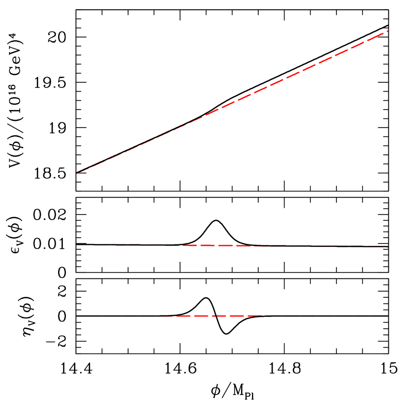
Figure 1 shows our fiducial inflationary potential, with parameters given in Table 1 that are chosen to fit the WMAP5 temperature glitches at as we will show in the next section. The number of -folds of inflation after the step in this potential is . The slow-roll parameters
| (10) |
are plotted in the lower panels of Fig. 1. Note that near the step at , confirming that the slow-roll approximation is not valid. Figure 2 shows the inflationary curvature power spectrum for this potential, computed by integrating Eqs. (6)(8).
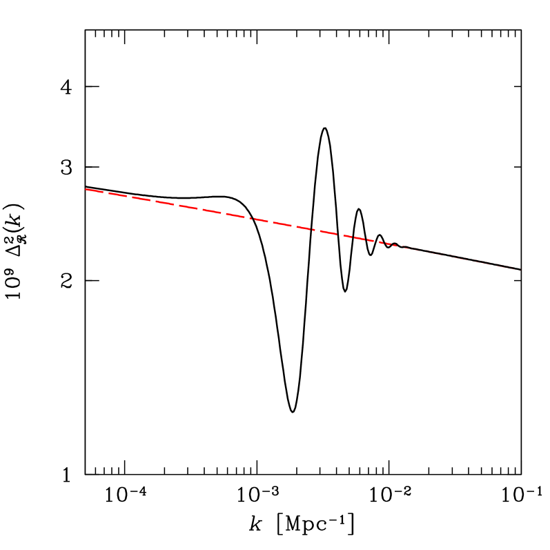
For comparison, in Figs. 1 and 2 we also show a smooth, potential with the same small-scale amplitude and tilt as the fiducial potential, and its slow-roll parameters and inflationary power spectrum. The smooth spectrum is nearly indistinguishable from a pure power law of with amplitude . Note that the spectral index is determined by the choices of and in the matching condition of Eq. (9), while the amplitude comes from the inflaton mass .
II.2 CMB Power Spectra
The mapping between the inflationary curvature power spectrum and the observable CMB angular power spectra
| (11) |
where , is given by the scalar radiation transfer functions
| (12) |
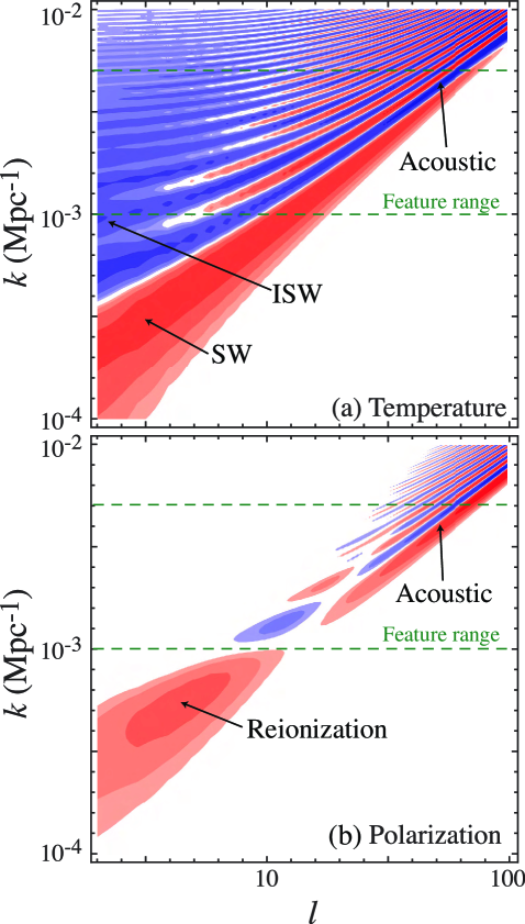
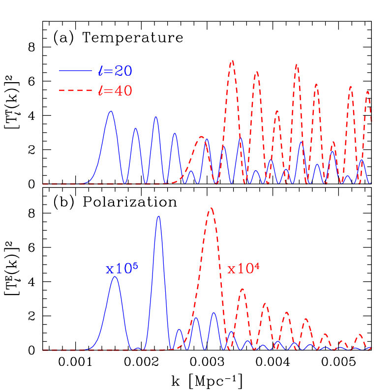
In Fig. 3, we show the and transfer functions for the fiducial cosmological parameters of Table 1. For a more extended discussion of the transfer functions and their relationship to features in the inflationary power spectrum, see Hu and Okamoto (2004). The resultant temperature and polarization angular power spectra from the inflationary power spectra of Fig. 2 are plotted in Fig. 4.
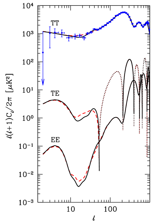
For the wavenumbers of interest, , the transfer of power to temperature fluctuations transitions between the Sachs-Wolfe and acoustic regimes at high and carries substantial contributions from the integrated Sachs-Wolfe (ISW) effect at low . These effects and geometric projection lead to a very broad mapping of power in to power in . In particular, the oscillations at the upper range in are largely washed out, leaving only a single broad dip at and bump at in the temperature spectrum. Likewise, the power at these multipoles correspond to a wide range in as shown in Fig. 5.
Polarization spectra differ notably from the temperature spectra due to the differences in the transfer function shown in Fig. 3. For the standard instantaneous reionization history and the upper portion of the range of affected by the feature, the polarization is dominated by the onset of acoustic effects only. We shall see that this makes the bump in a particularly clean test of inflationary features (see Fig. 5). Furthermore oscillations from high at higher are retained at a significant level in the polarization.
On the other hand at Mpc-1, the polarization transfer from recombination becomes very inefficient and reionization effects come into play. This leads to a very low level of polarization around with features even for a smooth inflationary power spectrum. These properties leave the dip vulnerable to external contamination such as tensor contributions (see § III.3) or foregrounds as well as uncertainties in the ionization history (see § IV).
Finally, the cross correlation between the temperature and polarization fields for the entire range of is very low due to the transition between the Sachs-Wolfe and acoustic-dominated regimes in the temperature field. We shall see in § III.4 that this prevents statistical fluctuations in the observed temperature power spectrum from being repeated in the polarization.
These differences in the transfer functions also play a role in defining the region in the potential parameter space that best fits the WMAP data versus the region that is best tested by polarization. For the former, we conduct a grid based search over the potential parameters. The mass parameter determines the amplitude of the spectrum away from the feature and so is mainly fixed by the acoustic peaks at high . The location of the feature is also well determined independently of the other parameters Covi et al. (2006); Hamann et al. (2007). We therefore fix and at their best-fit values and search for the best fit in the step amplitude and width parameters and .
The values of , , , and given in Table 1 specify the maximum likelihood model. This model improves the fit to the 5-year WMAP data by . We will explore variations in the parameters about the maximum and their relationship to the temperature and polarization power spectra through the transfer functions in § III.2.
The improvement is only marginally significant given the 3 extra parameters of the step and the choice of one out of many possible forms. Matching polarization features can therefore provide a critical confirmation or refutation of the inflationary nature of the temperature features.
III Confirming Features with Polarization
In this section, we discuss the significance with which polarization measurements can confirm or rule out the inflationary features discussed in the previous section under the instantaneous reionization model. We begin in § III.1 with the significance of the best-fit feature model under the simplest set of assumptions. We assess changes in the significance due to variation in the potential parameters in § III.2, and due to the inclusion of tensor -modes in § III.3. In § III.4, we describe the impact of conditioning polarization predictions on the already-measured temperature spectrum.
III.1 Fiducial Polarization Significance
To evaluate the significance of discriminating between models, we assume a Gaussian likelihood for the polarization angular power spectrum. In the absence of detector noise, the likelihood of data given a model power spectrum is
| (13) |
where is the fraction of sky with usable measurements. If the data have no inflationary feature and the model has the inflationary feature, we call this the significance at which false positives can be rejected. Conversely, if the data have an inflationary feature and the model spectrum has no feature, we call this the significance at which false negatives can be rejected.
| Experiment | ||||
|---|---|---|---|---|
| Ideal | — | 0 | 0 | 0.8 |
| Planck | GHz | |||
| GHz | ||||
| GHz |
For forecasts throughout this paper, we assume that the data are equal to the ensemble average of realizations for a particular model. Therefore, the minimum is zero and . The exception to this is that when we discuss the WMAP likelihood, the relevant quantity is where the likelihood of the best fit model is . We make forecasts for an ideal, sample variance limited experiment and for Planck using the experimental specifications in Table 2. For the Planck case with a finite noise power , in Eq. (13), where is the minimum variance combination of the noise powers of the individual frequency channels
| (14) |
using and from Table 2 converted to the appropriate units.
| Experiment | Test | |
|---|---|---|
| Ideal | False positive | |
| Ideal | False negative | |
| Planck | False positive | |
| Planck | False negative |
Table 3 lists for rejecting false positives and false negatives. The significance of false positive or negative rejection in this most optimistic case is for the ideal experiment and for Planck. In the following sections, we will discuss various effects that can degrade this significance.
III.2 Potential Parameters
Variation in the parameters of the inflationary potential from the best fit model can affect the significance of polarization tests of features. As noted in § II.2, and are strongly constrained by the observed CMB temperature spectrum, but the parameters and that control the amplitude and width of an inflationary step are less well determined by temperature alone.
In terms of the curvature power spectrum, increasing increases the amplitude of the features. However, decreasing the width of the potential step by lowering enhances the deviations from slow roll, thereby also amplifying the feature in the power spectrum.
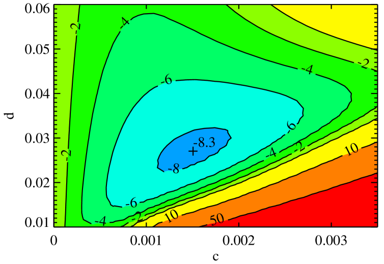
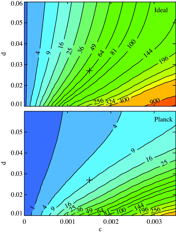
Figure 6 shows a contour plot of the WMAP temperature likelihood for the parameters and (relative to ) and Fig. 7 shows for false positives using simulated polarization data. The similarities and differences between these two plots reflect properties of the temperature and polarization transfer functions.
For the temperature case near the minimum, the degeneracy between the two parameters is approximately . This line roughly corresponds to keeping the amplitude of the enhanced power in at Mpc-1 fixed. The preferred value of corresponds to the best amplitude of the negative dip at Mpc-1. For the best fit parameters, including the feature in improves the fit to 5-year WMAP data by .
Due to the weak significance of the feature detection, the contours become substantially distorted away from the maximum likelihood. In particular, the contours in Fig. 6 show a triangular region extending to high . This region corresponds to a lower amplitude in both the first dip and bump in as shown in Fig. 8. Due to projection effects in temperature, the dip gets contributions from both the dip and the bump in (see Fig. 5). Consequently, a model with smaller features in in both the dip and bump can lead to the same amplitude of the dip at if the amplitude of the bump is reduced more.
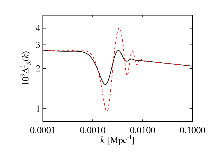
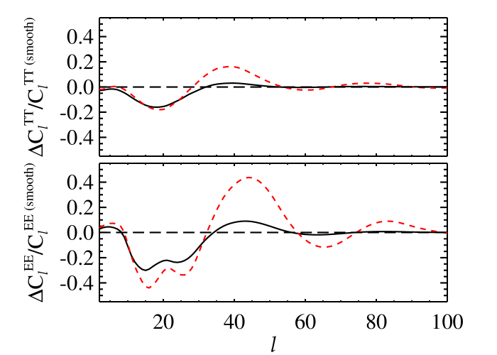
We illustrate these projection effects in Figs. 8 and 9 with two models chosen to have the same likelihood improvement of . For the model with smaller features in , the temperature enhancement at is substantially reduced compared with the best-fit model, while the model with larger features in overshoots the bump at in temperature. Despite these differences, both models have about the same amplitude in the dip as the best-fit model but a slightly worse overall fit. In particular, for the model with smaller features in , inflationary features can only explain the observed dip in temperature and not the bump.
The degeneracies in and for polarization significance share similarities with, yet have important differences from, those for temperature. The polarization significance remains largely unchanged for small variations in and along the constant line favored by the temperature spectra. Near the maximum, variations along this direction preserve the amplitude of intrinsic features in (see Fig. 6). However within the region the significance for a ideal experiment can either drop or rise significantly. The reason is that due to projection effects in temperature, the polarization better separates changes in the overall and relative amplitude of the features in . In the triangular high region, where the amplitude of the dip remains unchanged but the intrinsic features in are all reduced, the significance of the polarization difference decreases markedly (see Fig. 9). Because of the sharper projection, even the dip in polarization is reduced. The net result is that the polarization significance is a stronger function of , which controls the overall amplitude, than the temperature significance.
Note that while the significance can be substantially degraded from our best fit assumptions, this is mainly because of the weak detection of a feature in the temperature spectrum itself. In cases where the polarization significance is greatly reduced, the temperature bump at cannot be explained by the inflationary features. In other words, polarization remains a robust probe of the inflationary nature of the bump across variations of the potential parameters.
III.3 Tensors
The potential with the parameters in Table 1 predicts substantial gravitational wave contributions with tensor-to-scalar ratio . Relative to a smooth- model without tensors, the model with a feature has extra distinguishing power due to the presence of -mode polarization. Because other forms for the potential can also be used as the smooth base on which to place the feature Hamann et al. (2007) we choose not to include tensors for most of our calculations. Moreover, a -mode detection would not be useful for discriminating features. The -mode amplitude is insensitive to features since the potential amplitude is left nearly unchanged by the step. Additionally, a small step in the potential is not expected to generate features in the CMB power spectra of tensor modes. Unlike the scalar spectrum whose shape is sensitive to the second slow-roll parameter , the shape of the tensor spectrum depends primarily on , which remains small at the step (see Fig. 1, Hamann et al. (2007)). In Fig. 10 we show the -mode prediction for and a pure power law tensor spectrum with tilt .
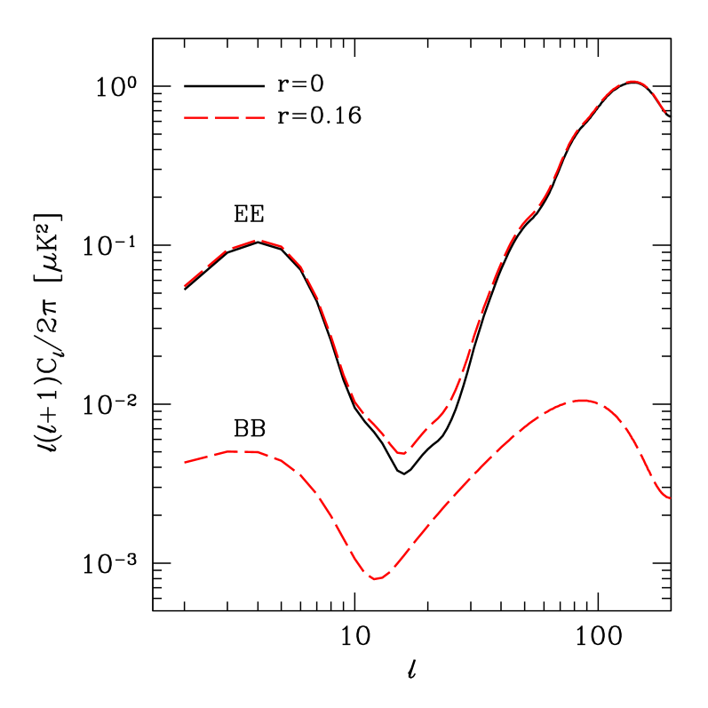
On the other hand, it is important to assess the possibility of degradation of the -mode feature from the curvature spectrum due to the nearly smooth tensor -mode contributions. Due to the shape of the tensor -mode spectrum, which mimics the -mode spectrum, the main impact of tensors is to fill in the dip in the polarization spectrum around (see Fig. 10). Correspondingly, the decrease in significance for the ideal experiment is in , and for Planck, . Planck is less affected since its lower sensitivity limits the accuracy of measurements in the dip. Since these degradations are relatively small, we ignore tensors when considering the impact of the reionization history below. Moreover, we shall see that reionization uncertainties are very similar to tensors in that they make the dip less useful for distinguishing features through -mode polarization.
III.4 Temperature Conditioning
The usefulness of polarization for providing an independent test of features observed in temperature may also be reduced by the correlation of temperature and polarization: a positive correlation would make observation of polarization features more likely given the WMAP data regardless of whether the features have an inflationary or chance statistical origin. We expect the reduction in significance to be small given that is small on the relevant angular scales (see Fig. 4), and in this section we quantify this statement.
To assess the impact of conditioning polarization predictions on the WMAP temperature data, it is convenient to replace the likelihood statistic of Eq. (13) with a statistic. This allows us to phrase the impact in terms of the bias and change in variance predicted for the power spectrum from the measurements. Note that in the absence of the temperature constraint and in the limit of small differences between the model and the data,
| (15) | |||||
which is equal to a simple statistic.
Now let us include the temperature constraint. First take the idealization that the temperature multipole moments have been measured on the full sky with negligible noise. Given a model that correlates the polarization field through the cross correlation coefficient
| (16) |
a constrained realization of the polarization field that is consistent with the temperature field can be constructed as
| (17) |
where is a complex Gaussian field with zero mean, unit variance , and a real transform . The estimate of the power spectrum is then
| (18) |
and its mean over the constrained realizations is biased from the true
| (19) |
by the fixed observed temperature power spectrum . With a high correlation coefficient, chance features in the temperature spectrum induce similar features in the observed polarization spectrum. For example, if fluctuates high, will also fluctuate high (on average).
The temperature constraint also removes some of the freedom in the variance of the polarization power spectrum:
| (20) | |||||
In the limit that the correlation , the variance takes on its usual form for a Gaussian random field. In the limit that , there is no uncorrelated piece and the observed temperature spectrum determines the observed polarization spectrum with no variance.
Now let us add in detector noise and finite sky coverage. Given a noise power spectrum and a fraction of the sky ,
| (21) |
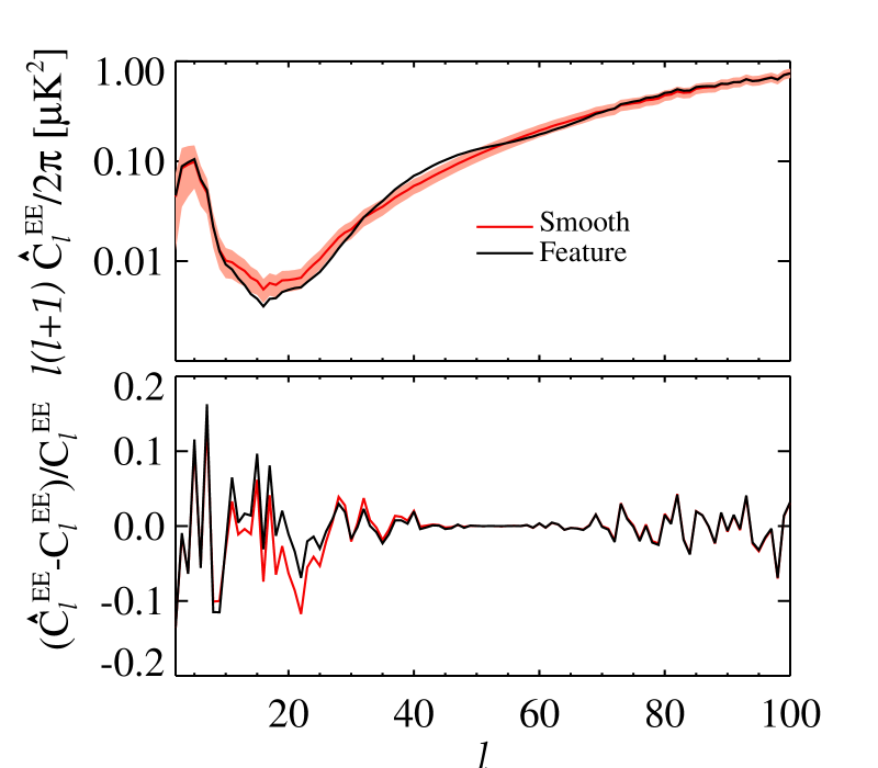
Figure 11 shows, in the upper panel, the -mode polarization power spectrum for the smooth inflationary spectrum constrained to WMAP5 temperature data for the ideal experiment. For comparison, for the best fit feature model is also plotted. Note that even the second dip in the spectrum at remains significantly distinct in polarization. In the lower panel, the impact of the temperature power spectrum constraint is plotted as the fractional difference between and for each model. Due to the lack of temperature-polarization correlation in the regime, the impact of the constraint on the polarization features is negligible.
We can quantify these conclusions by generalizing the statistic in Eq. (15) to include the temperature constraint:
| (22) |
As in the likelihood analysis, we assume that the data are a typical draw of the true model (“1”) and that we are testing the significance at which the second model (“2”) can be rejected. Then we set , , and Var()= Var(). Note that the bias induced by the temperature constraint enters into both models whereas the change in the variance enters only from model 2.
| Experiment | Test | w/o | with |
|---|---|---|---|
| Ideal | False positive | ||
| Ideal | False negative | ||
| Planck | False positive | ||
| Planck | False negative | ||
Table 4 assesses the significance of the rejection of false positives and false negatives for the fiducial feature model. In the last column we have applied the constraint from the WMAP5 temperature data and in the penultimate column we artificially drop the constraint by setting in the evaluation of . Even with the constraint, the significance with which false positives can be rejected is for the ideal experiment and for Planck. For the case of false negatives, these numbers become for the ideal experiment and for Planck. The difference between false positive and false negative significances comes from the dependence of sample variance on the model tested. In all cases, the significance in terms of is comparable to in Table 3.
The impact of the temperature constraint is to lower the significance of both cases but only by in . This small difference in significance justifies our choice to omit the constraint to temperature in our exploration of other effects that can degrade the significance.
IV Reionization Features
A more complicated ionization history can in principle produce features in the polarization spectrum that might mimic or obscure features from the inflationary power spectrum. This is especially true for the dip at . In this section we search for ionization histories that lead to a higher incidence of false positives and false negatives.
Reduced significance of false positives or negatives due to confusion between features from inflation and from reionization can arise in two ways. First, the true reionization history can introduce features in the data that either falsely mimic inflationary features or hide true features. Second, additional reionization freedom in the (false) model we wish to test can allow a better match to data generated from the alternate (true) model assumption. To account for both effects, we use a two-step method in which we first optimize the ionization history of the true model to produce a false positive or negative result, and then vary the ionization history of the false model. We will describe this procedure in § IV.2.
Table 5 summarizes the results of this section. Relative to the significance of rejecting false positives or negatives for instantaneous reionization models, ionization freedom lowers the significance for an ideal experiment by a factor of to , and for Planck by a substantially smaller factor of to . Given the amount of freedom we allow in the ionization history these should be viewed as the maximal degradation possible due to reionization. We describe the details of this calculation in the following sections.
| Experiment | Test | |
|---|---|---|
| Ideal | False positive | 36 |
| Ideal | False negative | 25 |
| Planck | False positive | 6 |
| Planck | False negative | 6 |
IV.1 Reionization Principal Components
The form of the ionization history, and therefore the shape of the large-scale reionization peak in the polarization spectrum, are only weakly constrained by current observations and theoretical modeling, especially on the scales relevant for inflationary features Mortonson and Hu (2008). We treat the evolution of the mean ionized fraction of hydrogen with redshift, , as an unconstrained function between and some high redshift . At lower redshifts, we assume as required by the observed Ly transmission in quasar spectra at (see e.g. Fan et al. (2006)). The highest redshift of reionization is less certain, so we take which is quite conservative for conventional sources of ionizing radiation.
We parametrize general reionization histories with a basis of principal components (PCs) of the large-scale -mode polarization Hu and Holder (2003). We use the 7 lowest-variance PCs only since the higher-variance PCs have a negligible impact on the polarization power spectrum. Thus the ionization history at is
| (23) |
where we take a constant fiducial ionized fraction of so that the fiducial model with has a total reionization optical depth of .
We vary the PC amplitudes and compare the resulting CMB power spectra with data simulated for ideal and Planck experiments using Markov Chain Monte Carlo (MCMC) likelihood analysis as we describe in the next section.
IV.2 Data and Model Optimization
We use a two-step optimization process to determine the maximum reduction in significance of false positive or negative rejection that can be caused by reionization features. We categorize models in this section by whether is smooth (S) or has a feature (F), and by whether the reionization history is instantaneous (I) or more complex (C) and parametrized by principal components as in Eq. (23). For comparisons of models we introduce the notation false:true; for example, FI:SI represents the false positive test for instantaneous reionization models from § III.
In the case of false positives, the goal of the optimization is to go from the FI:SI comparison of the previous section to FC:SC, in which both false and true models have complex ionization histories. In particular, we want to find the FC:SC pair that minimizes the difference between the two models, thus minimizing the significance of false positive rejection. To find this optimal pair of models, we use the following procedure:
-
1.
Optimize true (S) model: FI:(SISC)
Vary the ionization history of the SI model to find the SC model that best matches FI. -
2.
Optimize false (F) model: (FIFC):SC
Taking the optimal SC model from step 1 as the true model used to generate simulated data, vary the ionization history of the FI model to find the FC model that matches the best-fit SC.
Then the significance of rejecting false positives including reionization freedom is computed for the optimal FC:SC pair, i.e. the maximum likelihood from step 2.
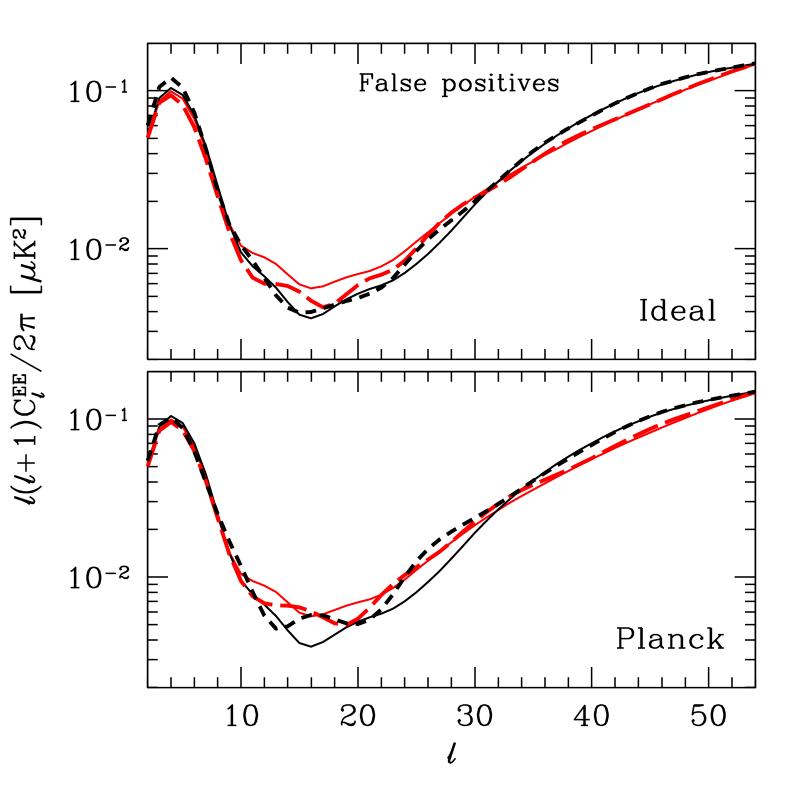
These steps for the false positive tests are illustrated in Fig. 12 for the ideal experiment. The process for false negatives can be described by simply swapping which models have features and which are smooth (F S).
Note that even with our conservative choice of , Fig. 12 shows that the main impact of reionization on the polarization spectra is limited to . We will explore the consequences of this restriction to large scales in the following section.
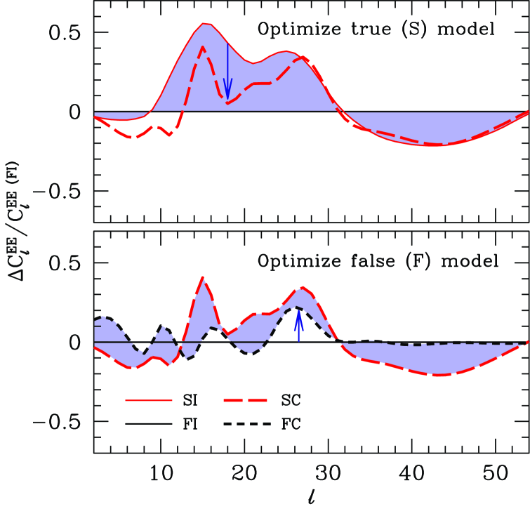
To implement the steps described above, we vary ionization histories to minimize following the methods of Refs. Mortonson and Hu (2008a, b); Mortonson and Hu (2008), using CosmoMC 111http://cosmologist.info/cosmomc/ Lewis and Bridle (2002) for MCMC likelihood analysis with a version of CAMB Lewis et al. (2000) modified to include reionization histories parametrized with principal components as in Eq. (23). For example, in the FI:(SISC) step above, we take the FI model as the simulated polarization data and search over ionization histories of the SC model class.
For each optimization step, we run 4 MCMC chains long enough to be well past any initial burn-in phase and stop when the region of parameter space near the best fit is sufficiently well sampled that all 4 chains agree on the maximum likelihood to within in . Typically this requires computing an initial chain to estimate the covariance matrix of the reionization PC amplitudes, followed by generating chains with samples each. The optimal true or false model is taken to be the overall maximum likelihood model from the final 4 chains.
All cosmological parameters besides the 7 reionization PC amplitudes are assumed to be fixed by measurements of the temperature spectrum, except for the amplitude of scalar fluctuations which is varied to keep fixed, preserving the temperature and polarization power at small scales. Fixed parameters are set to the values in Table 1. We use top-hat priors on the PC amplitudes corresponding to as described in Ref. Mortonson and Hu (2008a). Note that the number of PCs used here is larger than the 3 to 5 needed for completeness in Ref. Mortonson and Hu (2008a) due to our choice of a larger maximum redshift.
Although we are interested in the ability of polarization data to test features appearing in the observed temperature spectrum, we include the contributions from the model and spectra as well as in the likelihood for MCMC. Keeping the temperature data in the likelihood ensures that we do not obtain models that fit the polarization spectrum well at the expense of changing the shape of . For example, ionization histories with sharp transitions in at high redshift can generate polarization power at to match inflationary features, but these models also add power to the temperature on similar scales through an enhanced Doppler effect Mortonson and Hu (2008a); Mortonson and Hu (2008). For the best-fit models, the contribution of temperature data to the likelihood is approximately constant: .
IV.3 Reionization Confusion
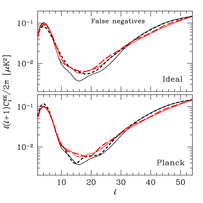
The optimal true and false model spectra obtained from the steps described in the previous section (SC and FC) are plotted in Figs. 13 and 14 for each of our 4 scenarios (ideal/Planck tests of false positives/negatives). We also plot the corresponding models with instantaneous reionization histories (SI and FI) to show where ionization freedom has the largest effect on the spectra. Table 5 lists for each FC:SC or SC:FC comparison.
The ability of reionization to either mimic or obscure the signature of inflationary features is greatest in the low-power regime of . For tests of false positives with an ideal experiment, nearly all of the reduction of due to reionization comes from . Planck, on the other hand, has relatively greater sensitivity to small changes in the polarization bump at since observations at such scales suffer less from instrumental noise than at . The reduction of for false positive rejection for Planck due to reionization is split equally between and . This fact combined with the weakness of reionization effects at makes Planck somewhat less sensitive to reionization uncertainties than an idealized noise-free experiment.
For false negative tests, changes to polarization spectra at are generally more important than they are for false positives. In the case of the ideal experiment, if we ignored multipoles above reionization would only reduce by relative to the instantaneous reionization significance instead of the reduction that we find when including all scales. The false model being tested in this case (smooth ) has less power and therefore lower sample variance at than the spectrum with a feature, and therefore changes in the polarization spectra on these scales have a greater effect on the significance than they do for false positive tests. Likewise, Planck’s significance is more dependent on the bump for testing false negatives than for false positives. In fact, nearly all of the degradation in for false negative rejection comes from for Planck.
Changes in the reionization history at are unable to significantly affect the polarization power spectrum at . A detection of polarization features on these scales would therefore be robust to reionization uncertainty. Likewise, measurement of a smooth spectrum on these scales would strengthen bounds on the height and width of a step in the inflaton potential.
By considering variations in up to , we include a wide variety of ionization histories, many of which may not be physically plausible. In practice, however, the ionization histories of the spectra in Figs. 13 and 14 have at . Nevertheless, had we chosen to limit ionization variation to lower redshifts the possibility of confusing reionization with inflationary features would be lessened, particularly for tests of false negatives and for Planck, due to the greater reliance on small-scale features in those cases.
Note that the effects of optimizing the ionization history and smoothing the polarization spectra with the addition of a large tensor component (§ III.3) are similar: both are able to make a spectrum with inflationary features and a smooth spectrum appear more alike at . Due to this similarity, we expect that considering tensors and reionization simultaneously would not further degrade the significance of false positive or negative tests.
For variations in the potential parameters discussed in § III.2 that retain only the dip at and not the bump at , the impact of reionization will be greater. In these cases one cannot expect polarization to provide unambiguous confirmation of features without external input on the ionization history.
V Discussion
Models with a step in the inflationary potential produce oscillations in the angular power spectra of the CMB that can improve the fit to WMAP temperature data at multipoles at the expense of 3 additional phenomenological parameters controlling the a step height, width, and location on the inflaton potential. Such models predict that these oscillations should appear in the -mode polarization spectrum on similar, few-degree scales. The first precise measurements of the polarization on these scales are anticipated in the next few years from Planck, enabling tests of the inflationary-step hypothesis.
Moreover, inflationary features at the upper range of ( Mpc-1) that are smoothed out due to projection effects in temperature should be more visible in polarization. For the lower range of ( Mpc-1), it becomes important to assess the impact of reionization and tensor mode uncertainties.
We have explored in detail the prospects for polarization tests of features, focusing in particular on the risk of errors that can be classified as false positives (falsely confirming an inflationary feature) and false negatives (falsely rejecting an inflationary feature). Under the simplest set of assumptions for large-scale polarization in which we take the best-fit model for the temperature features, neglect tensor fluctuations, and take the reionization history to be instantaneous, polarization measurements from Planck should be able to confirm or exclude the inflationary features that best match current temperature data with a significance of . All-sky experiments beyond Planck could potentially increase this significance to , providing a definitive test for features from inflation.
The estimated significance degrades slightly with the addition of a large-amplitude, smooth tensor component to the -mode spectrum, which tends to hide the effect of an inflationary step at the largest scales. Assuming that the step modifies an potential, is reduced by for Planck and for a cosmic variance limited experiment. Allowing non-standard reionization histories with arbitrary changes to the ionized fraction at can lower by as much as for Planck and for cosmic variance limited data. Since tensor fluctuations and reionization have the greatest impact on detectability of inflationary features at similar scales (), their effects on the significance should not be cumulative.
The possible contamination due to tensors or reionization could eventually be mitigated with constraints from other types of observations, e.g. stronger limits on the tensor-to-scalar ratio from the -mode polarization power spectrum. The -mode contribution from an potential is potentially within the reach of Planck Efstathiou et al. (2009). Note, however, that a failure to reject false positives or negatives for inflationary features in -mode polarization would generally bias the inferred ionization history and reionization parameters such as the optical depth. Such biases would in turn lead to biased constraints on inflationary parameters from tensor -mode measurements Mortonson and Hu (2008b).
These estimated significances assume that the parameters of the step in the inflaton potential are those that best fit the WMAP temperature spectrum. Away from this best fit, the polarization significance can either increase or decrease. Cases where the significance substantially decreases correspond to parameter combinations where at most one of the dip () and bump () temperature features can be explained by the step in the potential. In the case that only the dip is inflationary, Planck will be unable to confirm the feature.
We have not computed the impact of foreground removal uncertainties on our results; in general one might expect our forecasts to degrade somewhat upon including them. However, recent studies for Planck Efstathiou et al. (2009) and a future dedicated polarization satellite mission Verde et al. (2006); Dunkley et al. (2008) indicate that foregrounds will not be a substantial problem in the relevant multipole range. Finally, we do not address the possibility that the features in the WMAP data arise from a systematic effect (cf. Appendix A). Nonetheless, if all of the features in the temperature power spectrum are inflationary, polarization should ultimately provide a statistically significant confirmation.
Acknowledgments: We thank Jan Hamann and Richard Easther for valuable conversations. MJM, CD and WH were supported by the KICP through the grant NSF PHY-0114422 and the David and Lucile Packard Foundation. MJM was additionally supported through the NSF GRFP. WH was additionally supported by the DOE through contract DE-FG02-90ER-40560. HVP was supported in part by Marie Curie grant MIRG-CT-2007-203314 from the European Commission, and by a STFC Advanced Fellowship. HVP thanks the Galileo Galilei Institute for Theoretical Physics for the hospitality and the INFN for partial support during the completion of this work.
Appendix A Relation to Prior Work
Our best-fit parameters for the WMAP temperature data (Table 1) differ from those found by previous studies of the same inflationary model in Refs. Covi et al. (2006); Hamann et al. (2007). We explain here the reasons for these discrepancies, which include the addition of data and changes in the likelihood code in going from 3-year to 5-year WMAP data, as well as differences in the computation of the evolution of modes during inflation.
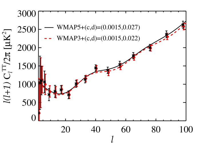
Due to small changes in the observed spectrum between WMAP 3-year and 5-year data, we find that the best-fit width of the feature increased from to a value of . The lower value of agrees with the best-fit value found by Ref. Hamann et al. (2007), which was based on the 3-year data. Note that a wider feature in implies a narrower feature in for the CMB power spectra. Fig. 15 shows the best fit models for both data sets along with the appropriately binned data.
Updates to the WMAP likelihood code could also cause small changes in the best-fit potential parameters. In fact, one might be concerned that the feature in the WMAP temperature data is only a systematic effect with some artificial origin in the likelihood calculation. In particular, given the location of a feature, its significance could emerge in some fashion from the transition between the low- pixel-based likelihood code and the high- harmonic space likelihood code, which happens at in the 5-year likelihood code Dunkley et al. (2009). However, in the original version of the 3-year likelihood code, v2p1, the transition occurred at , and in the final version, v2p2p2, it was changed to Hinshaw et al. (2007). We searched for the best-fit feature model using WMAP3 data with these two versions of the likelihood code and found almost exactly the same values for the potential parameters in both cases, indicating that this particular issue is not the source of a systematic effect.
Our best fit value for is considerably different from Refs. Covi et al. (2006); Hamann et al. (2007) even though we use the same matching condition as they do between -folds and physical wavenumbers. This is due to a choice of initial conditions for the background evolution of the inflaton by these authors that did not quite satisfy the Friedmann equation, with the result that the subsequent evolution also failed to satisfy it Hamann (2009). This essentially translates into a horizontal shift in , changing the preferred location of the step .
Ref. Hamann et al. (2007) discusses relaxing the model dependence of the predicted power spectrum from the chaotic inflation “toy model” adopted here by using a free spectral index that is fit to the data rather than set by the choice of . Since the value of determined by our matching condition for the chaotic inflation potential as described in § II is nearly identical to the spectral tilt in the WMAP5 best-fit concordance model (i.e. with smooth ), we do not carry out this extra step here. However, the form of the underlying potential will be tested by the Planck satellite irrespective of the existence of features; as we note in § III.3, the tensor amplitude predicted by the potential (which is not affected by the presence of the feature) is within Planck’s reach Efstathiou et al. (2009).
References
- Hinshaw et al. (2009) G. Hinshaw et al., Astrophys. J. Suppl. 180, 225 (2009), eprint arXiv:0803.0732.
- Bennett et al. (2003) C. L. Bennett et al., Astrophys. J. Suppl. 148, 1 (2003), eprint astro-ph/0302207.
- Dunkley et al. (2009) J. Dunkley et al., Astrophys. J. Suppl. 180, 306 (2009), eprint arXiv:0803.0586.
- Nolta et al. (2009) M. R. Nolta et al., Astrophys. J. Suppl. 180, 296 (2009), eprint arXiv:0803.0593.
- Komatsu et al. (2009) E. Komatsu et al., Astrophys. J. Suppl. 180, 330 (2009), eprint arXiv:0803.0547.
- Peiris and Easther (2008) H. V. Peiris and R. Easther, JCAP 0807, 024 (2008), eprint arXiv:0805.2154.
- Kinney et al. (2008) W. H. Kinney, E. W. Kolb, A. Melchiorri, and A. Riotto, Phys. Rev. D78, 087302 (2008), eprint arXiv:0805.2966.
- Alabidi and Lidsey (2008) L. Alabidi and J. E. Lidsey, Phys. Rev. D78, 103519 (2008), eprint arXiv:0807.2181.
- Lesgourgues and Valkenburg (2007) J. Lesgourgues and W. Valkenburg, Phys. Rev. D75, 123519 (2007), eprint astro-ph/0703625.
- Spergel et al. (2007) D. N. Spergel et al., Astrophys. J. Suppl. 170, 377 (2007), eprint astro-ph/0603449.
- Parkinson et al. (2006) D. Parkinson, P. Mukherjee, and A. R. Liddle, Phys. Rev. D73, 123523 (2006), eprint astro-ph/0605003.
- Gordon and Trotta (2007) C. Gordon and R. Trotta (2007), eprint arXiv:0706.3014.
- Verde and Peiris (2008) L. Verde and H. V. Peiris, JCAP 0807, 009 (2008), eprint arXiv:0802.1219.
- Bridges et al. (2008) M. Bridges, F. Feroz, M. P. Hobson, and A. N. Lasenby (2008), eprint arXiv:0812.3541.
- Spergel et al. (2003) D. N. Spergel et al., Astrophys. J. Suppl. 148, 175 (2003), eprint astro-ph/0302209.
- Peiris et al. (2003) H. V. Peiris et al., Astrophys. J. Suppl. 148, 213 (2003), eprint astro-ph/0302225.
- Hannestad (2004) S. Hannestad, JCAP 0404, 002 (2004), eprint astro-ph/0311491.
- Shafieloo and Souradeep (2004) A. Shafieloo and T. Souradeep, Phys. Rev. D70, 043523 (2004), eprint astro-ph/0312174.
- Mukherjee and Wang (2003) P. Mukherjee and Y. Wang, Astrophys. J. 599, 1 (2003), eprint astro-ph/0303211.
- Shafieloo et al. (2007) A. Shafieloo, T. Souradeep, P. Manimaran, P. K. Panigrahi, and R. Rangarajan, Phys. Rev. D75, 123502 (2007), eprint astro-ph/0611352.
- Nicholson and Contaldi (2009) G. Nicholson and C. R. Contaldi (2009), eprint arXiv:0903.1106.
- Starobinsky (1992) A. A. Starobinsky, JETP Lett. 55, 489 (1992).
- Adams et al. (2001) J. A. Adams, B. Cresswell, and R. Easther, Phys. Rev. D64, 123514 (2001), eprint astro-ph/0102236.
- Joy et al. (2008a) M. Joy, V. Sahni, and A. A. Starobinsky, Phys. Rev. D77, 023514 (2008a), eprint arXiv:0711.1585.
- Silk and Turner (1987) J. Silk and M. S. Turner, Phys. Rev. D35, 419 (1987).
- Holman et al. (1991) R. Holman, E. W. Kolb, S. L. Vadas, and Y. Wang, Phys. Lett. B269, 252 (1991).
- Polarski and Starobinsky (1992) D. Polarski and A. A. Starobinsky, Nucl. Phys. B385, 623 (1992).
- Adams et al. (1997) J. A. Adams, G. G. Ross, and S. Sarkar, Nucl. Phys. B503, 405 (1997), eprint hep-ph/9704286.
- Hunt and Sarkar (2004) P. Hunt and S. Sarkar, Phys. Rev. D70, 103518 (2004), eprint astro-ph/0408138.
- Lesgourgues (2000) J. Lesgourgues, Nucl. Phys. B582, 593 (2000), eprint hep-ph/9911447.
- Burgess et al. (2005) C. P. Burgess, R. Easther, A. Mazumdar, D. F. Mota, and T. Multamaki, JHEP 05, 067 (2005), eprint hep-th/0501125.
- Ashoorioon and Krause (2006) A. Ashoorioon and A. Krause (2006), eprint arXiv:hep-th/0607001.
- Covi et al. (2006) L. Covi, J. Hamann, A. Melchiorri, A. Slosar, and I. Sorbera, Phys. Rev. D74, 083509 (2006), eprint astro-ph/0606452.
- Hamann et al. (2007) J. Hamann, L. Covi, A. Melchiorri, and A. Slosar, Phys. Rev. D76, 023503 (2007), eprint astro-ph/0701380.
- Hunt and Sarkar (2007) P. Hunt and S. Sarkar, Phys. Rev. D76, 123504 (2007), eprint arXiv:0706.2443.
- Joy et al. (2008b) M. Joy, A. Shafieloo, V. Sahni, and A. A. Starobinsky (2008b), eprint arXiv:0807.3334.
- Martin and Ringeval (2004) J. Martin and C. Ringeval, Phys. Rev. D69, 083515 (2004), eprint astro-ph/0310382.
- Kawasaki et al. (2005) M. Kawasaki, F. Takahashi, and T. Takahashi, Phys. Lett. B605, 223 (2005), eprint astro-ph/0407631.
- Jain et al. (2009) R. K. Jain, P. Chingangbam, J.-O. Gong, L. Sriramkumar, and T. Souradeep, JCAP 0901, 009 (2009), eprint arXiv:0809.3915.
- Hu and Okamoto (2004) W. Hu and T. Okamoto, Phys. Rev. D69, 043004 (2004), eprint astro-ph/0308049.
- Kogo et al. (2004) N. Kogo, M. Sasaki, and J. Yokoyama, Phys. Rev. D70, 103001 (2004), eprint astro-ph/0409052.
- Pahud et al. (2009) C. Pahud, M. Kamionkowski, and A. R. Liddle, Phys. Rev. D 79, 083503 (2009), eprint arXiv:0807.0322.
- Nagata and Yokoyama (2009) R. Nagata and J. Yokoyama, Phys. Rev. D79, 043010 (2009), eprint arXiv:0812.4585.
- Dore et al. (2004) O. Dore, G. P. Holder, and A. Loeb, Astrophys. J. 612, 81 (2004), eprint astro-ph/0309281.
- Skordis and Silk (2004) C. Skordis and J. Silk (2004), eprint astro-ph/0402474.
- Gordon and Hu (2004) C. Gordon and W. Hu, Phys. Rev. D70, 083003 (2004), eprint astro-ph/0406496.
- Fang et al. (2008) W. Fang et al., Phys. Rev. D78, 103509 (2008), eprint arXiv:0808.2208.
- Hu and Holder (2003) W. Hu and G. P. Holder, Phys. Rev. D68, 023001 (2003), eprint astro-ph/0303400.
- Mortonson and Hu (2008a) M. J. Mortonson and W. Hu, Astrophys. J. 672, 737 (2008a), eprint arXiv:0705.1132.
- Mortonson and Hu (2008b) M. J. Mortonson and W. Hu, Phys. Rev. D77, 043506 (2008b), eprint arXiv:0710.4162.
- The Planck Collaboration (2006) The Planck Collaboration (2006), eprint astro-ph/0604069.
- Baumann et al. (2008) D. Baumann et al. (2008), eprint arXiv:0811.3919.
- Dvorkin et al. (2008) C. Dvorkin, H. V. Peiris, and W. Hu, Phys. Rev. D77, 063008 (2008), eprint arXiv:0711.2321.
- Leach and Liddle (2001) S. M. Leach and A. R. Liddle, Phys. Rev. D63, 043508 (2001), eprint astro-ph/0010082.
- Mukhanov (1988) V. F. Mukhanov, Zhurnal Eksperimental noi i Teoreticheskoi Fiziki 94, 1 (1988).
- Sasaki (1986) M. Sasaki, Progress of Theoretical Physics 76, 1036 (1986).
- Stewart and Lyth (1993) E. D. Stewart and D. H. Lyth, Physics Letters B 302, 171 (1993), eprint gr-qc/9302019.
- Mukhanov (1985) V. F. Mukhanov, JETP Lett. 41, 493 (1985).
- Mukhanov et al. (1992) V. F. Mukhanov, H. A. Feldman, and R. H. Brandenberger, Phys. Rep. 215, 203 (1992).
- Mortonson and Hu (2008) M. J. Mortonson and W. Hu, Astrophys. J. Lett. 686, L53 (2008), eprint 0804.2631.
- Fan et al. (2006) X.-H. Fan, C. L. Carilli, and B. G. Keating, Ann. Rev. Astron. Astrophys. 44, 415 (2006), eprint astro-ph/0602375.
- Lewis and Bridle (2002) A. Lewis and S. Bridle, Phys. Rev. D66, 103511 (2002), eprint astro-ph/0205436.
- Lewis et al. (2000) A. Lewis, A. Challinor, and A. Lasenby, Astrophys. J. 538, 473 (2000), eprint astro-ph/9911177.
- Efstathiou et al. (2009) G. Efstathiou, S. Gratton, and F. Paci (2009), eprint arXiv:0902.4803.
- Verde et al. (2006) L. Verde, H. Peiris, and R. Jimenez, JCAP 0601, 019 (2006), eprint astro-ph/0506036.
- Dunkley et al. (2008) J. Dunkley et al. (2008), eprint arXiv:0811.3915.
- Hinshaw et al. (2007) G. Hinshaw et al., Astrophys. J. Suppl. 170, 288 (2007), eprint astro-ph/0603451.
- Hamann (2009) J. Hamann (2009), private communication.