Growing correlations and aging of an elastic line in a random potential
Abstract
We study the thermally assisted relaxation of a directed elastic line in a two dimensional quenched random potential by solving numerically the Edwards-Wilkinson equation and the Monte Carlo dynamics of a solid-on-solid lattice model. We show that the aging dynamics is governed by a growing correlation length displaying two regimes: an initial thermally dominated power-law growth which crosses over, at a static temperature-dependent correlation length , to a logarithmic growth consistent with an algebraic growth of barriers. We present a scaling arguments to deal with the crossover-induced geometrical and dynamical effects. This analysis allows to explain why the results of most numerical studies so far have been described with effective power-laws and also permits to determine the observed anomalous temperature-dependence of the characteristic growth exponents. We argue that a similar mechanism should be at work in other disordered systems. We generalize the Family-Vicsek stationary scaling law to describe the roughness by incorporating the waiting-time dependence or age of the initial configuration. The analysis of the two-time linear response and correlation functions shows that a well-defined effective temperature exists in the power-law regime. Finally, we discuss the relevance of our results for the slow dynamics of vortex glasses in High-Tc superconductors.
pacs:
74.25.Qt,75.60.Ch,64.70.kj,64.60.HtI Introduction
Disordered elastic manifolds play an important role in a variety of physical systems. Growing surfaces, Barabasi-Stanley interfaces in domain growth phenomena and phase separation, Alan and cracks in brittle materials cracks are usually viewed as elastic objects. Interesting one dimensional realizations are polymers polymers and vortex flux lines in type II superconductors. rusos While polymers can wrap, vortex flux lines are preferentially directed along the applied magnetic field.
A number of systems involving one dimensional elastic manifolds display glassy features. An ensemble of interacting polymers forms a polymer melt that undergoes a glass transition. polymers The competition between vortex repulsion and their pinning to randomly located impurities also leads to glassy phases in superconductors. rusos While in the former case disorder is self-induced, in the latter the effect of the impurities is mimicked by a quenched random potential.
The relaxation dynamics of a model of layered high superconductors was recently studied in Ref. us, . The magnetic vortices are considered to be directed along one direction and they can move in two transverse directions. Conventionally, this is a + dimensional model. The dynamics following a rapid quench from the liquid state to a set of control parameters in which the equilibrium state is expected to be the so-called ‘vortex glass’ rusos was monitored. By using numerical simulations a slow out of equilibrium relaxation typical of glasses was found. In this system, diffusive aging of the averaged two-time roughness, , and displacement, , was observed. The aging was characterized by a multiplicative scaling form , where is a growing characteristic length. The scaling functions and are different but the exponent does not depend on the observable ( or ). Besides, the system of interacting lines was perturbed in order to compute the integrated linear response, and a diffusive aging was also found, characterized by a scaling function of the type with the same exponent and growing length found for the unperturbed two-time observables (roughness and displacement). It was also shown that correlation and response functions can be related by a modified fluctuation-dissipation relation after removing the ‘diffusive’ contribution, i.e. the factors . This violation of the fluctuation-dissipation relation can be characterized by a finite effective temperature, . Cukupe ; Leto Furthermore, within the time-window that was numerically explored, the growing length is well-described by a power-law, . This could well be a pre-asymptotic regime after which the growing length crosses over to the expected activated dynamics logarithmic growth (when disorder free-energy barriers scale as with ). It is worth to mention that although aging in high high-Tc and low low-Tc superconductor samples has been reported in the literature, a detailed comparison to the results listed above remains to be done.
The model system used to describe vortex lines in high temperature superconductors contains several contributions coming from different energy scales. The main contributions are: the elastic energy of the individual lines, non-linear terms in the elastic energy, the interaction between the lines, and the quenched random pinning potential. It is clearly important to establish whether all the above listed contributions to the energy are necessary to get such aging behavior or whether similar features arise when some of the terms – non-linear contributions to the elasticity, interactions between the lines, random potential – are switched off. We review below the out of equilibrium dynamics of related models with and without this type of interactions.
The first studies of the out of equilibrium dynamics of directed elastic manifolds in a quenched random environment focused on mean-field models in which the transverse space is infinitely dimensional, , each transverse coordinate has infinite length, , and the manifold has finite dimension, , and infinite length in all directions, . Cule This model includes only two of the energetic contributions listed above viz. elasticity and quenched disorder and neglects non-linear terms and interactions between the elastic objects. A dynamic phase transition separating a liquid (high-temperature) phase from a glassy (low-temperature) one was found for all internal dimension including . Cule Different aging dynamics characterize the low-temperature phase depending on the short or long range character of the random potential correlations. In both cases the aging regime lasts for ever (after having taken the , and limits): there is no multiplicative factor in the averaged two-time observables. For short-range correlated potentials the displacement, roughness and linear responses scale as and a single finite effective temperature exists.
Soon after Barrat Barrat and Yoshino Yoshino ; Yoshino-unp studied a solid-on-solid model of a single directed elastic line relaxing with Monte Carlo dynamics on a disordered substrate with one () transverse direction. This system models elasticity in a rather extreme way, using a hard constrain, and includes quenched randomness. There are no interaction between different lines in this model. These authors focused on the very long length limit in an effectively infinite box ( with the lattice spacing) and found that this lattice model has a similar averaged dynamics to the one found later in the vortex glass us below a crossover temperature. The relaxation is slow, and the global displacement and linear response show non-trivial diffusive aging with multiplicative scaling. The characteristic length scale also appears to be a power-law of time within the numerical time window and the exponents and are temperature and disorder strength dependent with the same qualitative trend as in the fully interacting case. More recently, we focused on the analysis of the averaged and fluctuating two-time roughness of such solid-on-solid lines with finite length, . EPL On the one hand, we found that the aging regime stops and crosses over to saturation of the two-time roughness and free diffusion of the displacement at a characteristic value of the time delay, , that grows with the length of the line and smoothly depends on other parameters in the model. The saturation of the two-time roughness is well described by a generalization of the equilibrium Family-Vicsek scaling. Favi On the other hand, the two-time roughness fluctuations are highly non-trivial but can be characterized with a relatively simple argument by a scaling function.
The numerical solution to the Langevin equation for free lines in transverse dimensions us and, especially, the full analytic solution to the Langevin dynamics of finite Edwards-Wilkinson (EW) elastic lines EW in one transverse dimension Sebastian ; Pleimling () had also been considered, without taking into account interactions, non-linear terms and quenched randomness. The results suggested that not even disorder is necessary to obtain similar averaged and fluctuating aging dynamics of fully relaxing quantities. The aging scaling and saturation phenomenon of the averaged two-time roughness follow the same scaling laws as above with growing length , and temperature-independent exponents , and . However, the noise-averaged linear response is stationary in this ‘quadratic’ model. When it comes to analyzing fluctuations other differences appear. The distribution of the two-time roughness satisfies a similar scaling law as in the disordered problem although with a rather different scaling function and the linear response simply does not fluctuate.
The effect of non-linear terms has been considered by Bustingorry Sebastian2 ; Spaniards who analyzed the relaxation dynamics of ‘clean’ finite length () Kardar-Parisi-Zhang (KPZ) lines KPZ in transverse dimensions. In this work correlations were analyzed in detail and undergo diffusive aging with the KPZ exponents , and . The two-time and length scaling of averaged quantities and the scaling form of the probability distribution functions proposed in Ref. EPL, were thus confirmed.
Finally, once the elastic lines are allowed to wrap, biologically motivated dynamic problems can also be addressed. A recent study concentrates on the effects of confinement on the out of equilibrium relaxation of a single polymer chain in two dimensions, claudio a problem of relevance for cellular modelling. Another study analyzes numerically the effect of randomly applied forces on an ensemble of interacting polymer lines, focusing on out of equilibrium properties of active matter. Davide There is, certainly, much room for further investigations in the biological context.
In this paper we return to the problem of the relaxation of directed elastic lines in the presence of quenched randomness. Interactions among different lines and non-linear terms are not considered here. Our aim is to complete the analysis of the averaged two-time observables. In order to compare with previous results and to extract the universal behaviour we treat two models in parallel: the Monte Carlo dynamics of the disordered solid-on-solid model Barrat ; Yoshino ; Yoshino-unp and the Langevin dynamics of the disordered Edwards-Wilkinson equation in dimensions. We present a careful study of finite-length effects on the averaged dynamics of correlation and linear response functions. We pay special attention to the behavior of the crossover length between thermal and disorder dominated regimes, and discuss finite-size and finite-time effects. Moreover, we show by using scaling arguments how this length scale determines the relaxation properties of the system.
The organization of the paper is the following. In Sect. II we define the models and we describe the numerical method and two-time observables on which we focus. In Sect. III we measure the growth, roughness and dynamic exponents by analyzing the two-time structure factor and two-time roughness. We also study in detail the growing length and we confirm the existence of a crossover from power-law to logarithmic growth that is, however, only seen for sufficiently long lines. Section IV summarizes the two-time behavior of the averaged roughness and associated linear response using different initial conditions. In Sect. V we present scaling arguments to explain many of the features observed numerically. Finally, in Sect. VI we present our conclusions.
II The models
In this section we introduce the models and the numerical methods used to study their relaxation.
II.1 Lattice model
A discrete model of a one-dimensional directed elastic object represents the line as a lattice string of length directed along the direction. Barrat ; Yoshino ; Yoshino-unp ; EPL The line can move transversely along the direction on a rectangular square lattice of transverse size ensuring the existence of many nearly equivalent, quasi-ground states. The line segments, (), obey the restricted solid-on-solid (SOS) rule . A quenched random potential taking independent values on each lattice site is drawn from a uniform distribution in . We use realizations of the quenched randomness depending on the value of . At each microscopic time step we attempt a move of a randomly chosen segment to one of its neighbors restricted by the SOS condition and we accept it with the heat-bath rule. One Monte Carlo (MS) step is defined as update attempts. We use angular brackets to indicate the average over thermal noise realizations. We choose two types of initial conditions: equilibrium at high temperature obtained after evolving a random initial condition during a sufficiently long time interval at high temperature, and equilibrium at zero temperature.
The lattice model has no finite elastic energy. Elasticity is modelled in an extreme way; in the absence of disorder all configurations have equal vanishing energy but the displacement between neighboring bonds is bounded to lattice spacings.
The control parameters are temperature, , and the disorder strength, . Here and in what follows we use square brackets, , to indicate an average over quenched randomness. The Monte Carlo rule implies that the dynamics depend only on the ratio between these parameters, . In the simulations shown here we fixed . In the following we use adimensional time, space and energy scales.
II.2 Continuous model
The SOS model is easy to simulate but it is not simply recovered as a limit of better-known continuous problems like the KPZ equation KPZ ; Sebastian2 or the vortex line model us in which elasticity is modelled in a more realistic way. For this reason we also study the disordered Edwards-Wilkinson (EW) line. Barabasi-Stanley
The disordered EW equation EW for a scalar field representing the height of a surface over a one dimensional substrate parametrized by the coordinate (a one dimensional directed interface) is
| (1) |
where is a Gaussian thermal noise with and
| (2) |
The parameter is the elastic constant, is the friction coefficient, the temperature of the thermal bath (in energy units) and the average over the white noise , i.e. the thermal average. The Boltzmann constant has been set to one, . The term represents the effect of a perturbing field that couples linearly and locally to the height, . One can also consider other types of perturbation that couple to more complicated functions of the height as defined in Sect. II.4. The random pinning force represents the effect of a random-bond disorder described by the potential , whose sample to sample fluctuations are given by
| (3) |
where stands for a short ranged correlator along the coordinate with range . The continuous random potential is modeled by a cubic spline passing through regularly spaced uncorrelated Gaussian number points. rosso_depinning_simulation We adimensionalize Eq. (1) by using as the unit of distance in the direction, as the unit of time, and as unit of energy/temperature. The unit of distance in the longitudinal direction can be conveniently taken as the layer spacing of the numerically discretized laplacian (such a choice is natural when modeling a layered material such as a High-Tc superconductor with an external magnetic field applied perpendicular to the oxide planes). In these units, the friction and elastic coefficients are equal to one, leaving only two independent parameters in the model: the adimensionalized elastic constant and the adimensionalized temperature (from now on, we use for ). Finally, by choosing we focus exclusively in the temperature dependence for a fixed disorder.
We use a finite-difference algorithm to integrate the partial differential equation in which the first and second order partial derivatives are discretized in the usual way. (See Ref. Sebastian2, for more details on the numerical technique.) We typically simulate lines with length . The time step is . We use noise realizations to evaluate the two-times averaged correlations and responses.
Note that in the continuous model each non strictly flat configuration has a finite elastic energy while in the lattice model all configurations have the same vanishing elastic energy.
II.3 Quenched randomness
The kind of quenched disorder used in both models is of the ‘random bond’ type in the sense that, for a domain wall described by our elastic interface model, it does not break the symmetry properties of the corresponding order parameter. Nattermann This implies that the two dimensional disorder potential locally couples to the interface position and that in Eq. (3) saturates to a constant for large distances. The way we generate the disorder corresponds to a short-ranged function . The effect of long-range correlated randomness has been studied in mean-field elastic manifold models Cule but we do not contemplate it here.
II.4 Observables
We study the relaxation after two types of rapid changes in the control parameters. The first protocol, and the more usual one, describes a quench from high to low temperatures. After equilibration at high the system is quenched to a low value of . The second protocol, less usual, consists in first equilibrating the sample at zero temperature (i.e. starting in its ground-state), , and then heating the sample to a higher temperature. In both cases, the line is allowed to relax from the quench occuring at time until a waiting-time , when the quantities of interest are recorded and later compared to their values at subsequents times .
The aging dynamics of elastic lines has been initially studied in terms of the averaged two-time mean-squared-displacement . Barrat ; Yoshino The behavior of this quantity is somehow obscured by the motion of the center of mass. We thus prefer to focus on the roughness of the lines, a quantity that has been widely used in the study of interface dynamics, Barabasi-Stanley but generalized here to include the and dependence. The two-time roughness is given by
| (4) |
where accounts for the displacement of the -th line segment relative to the center of mass, .
Further insight into the dynamics of out of equilibrium systems is given by the linear response function. The latter is defined by applying a random time-independent force at a time on a replica of the system, and by computing how this one departs from an unperturbed one evolving with the same thermal noise. Concretely, the energy contribution of a field conjugated to the displacement with respect to its mean value is
| (6) |
with equal probability, and Kolton-us with denoting the average over the perturbing field distribution. is the intensity of the perturbation. The associated linear response function is
| (7) |
Henceforth indicates the average over the thermal noise and the distribution.
In equilibrium the averaged linear response is related to the averaged spontaneous fluctuations of the corresponding observable by the model-independent fluctuation-dissipation theorem (FDT) which states
| (8) |
(the Boltzmann constant has been set to one, ), where the argument implies stationary dynamics. In a system relaxing out of equilibrium this relation does not necessarily hold. In a number of glassy systems one can define an effective temperature Cukupe from the modification of the above relation. In the aging regime of elastic lines in disorder media the FDT is violated and one constructs the modified FDT Leto ; Yoshino ; us
| (9) |
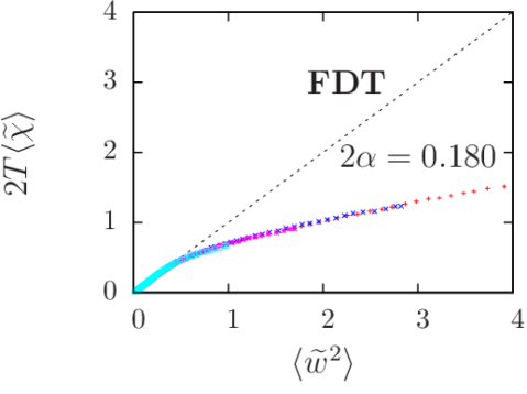
The two-time dependence of the effective temperature is here kept general. It turns out that in models with multiplicative scaling, as the one discussed here, once the factors have been taken into account, the re-defined effective temperature approaches a constant value (see Sect. IV.3 and Refs. Barrat, ; Yoshino, ; Yoshino-unp, ; us, ; Sebastian, ; Kolton-us, ).
II.5 Dynamic crossover
In dimensional models of elastic manifolds the glassy phenomenon appears as a dynamic crossover. Barrat ; Yoshino ; Yoshino-unp ; EPL ; Sebastian ; Pleimling ; Sebastian2
For all observation times, , that are longer than a size, disorder-strength and temperature dependent equilibration time, , the system reaches equilibrium. Instead, for the relaxation is non-stationary and thus occurs out of equilibrium as demonstrated by two-time correlations and linear responses that age and by a non-trivial relation between them.
The equilibration time increases by increasing the size of the line, by decreasing the temperature , and by increasing the quenched disorder strength . At fixed disorder strength and line length the dynamic crossover reflects in a temperature crossover that resembles a phase transition at a characteristic temperature . At high temperature, , the equilibration time is short, disorder is irrelevant and the line behaves as the clean EW one at high temperature: the dynamics of a finite length line reaches equilibrium meaning that stationary dynamics and the FDT hold, and the exponents (defined and discussed below) are the ones of the clean EW line, , and . At lower temperatures, , the equilibration time is longer than the observation time and the dynamics remains non-stationary. Barrat ; Yoshino ; Yoshino-unp ; EPL Quenched disorder modifies the values of the exponents and induces a geometrical crossover at a temperature dependent length-scale , from a short length-scale roughness described by the ‘thermal’ exponent , to a large length-scale roughness described by a ‘disorder’ exponent . We shall discuss the values of the exponents and the out of equilibrium dynamics in the following sections.
III Growth and saturation
In this Section we recall the main tools used to analyze the evolution of the conformational properties of elastic manifolds and we generalize them to take into account the effect of the waiting-time. This leads us to present the temperature dependence of the crossover length scale .
III.1 Roughness
III.1.1 Comparison to the initial condition
Traditionally, the dynamics of elastic manifolds has been classified in universality classes according to the behavior of the two-time roughness (4) evaluated at , the initial time, and using a flat initial configuration, . Barabasi-Stanley ; Favi The waiting-time being identical to zero all two-time observables depend on when compared to the initial condition. Initially the roughness increases as a function of , and at a characteristic time reaches saturation at an -dependent value, . This behavior is encoded in the Family-Vicsek scaling Favi that, in full generality, can be expressed as
| (10) | |||||
| (11) | |||||
| (12) |
with three monotonic functions. Consistency at requires . In the usually discussed space-time scale-invariant cases in which all functions are power-laws one has
| (13) | |||||
| (14) | |||||
| (15) |
with the growth exponent, the dynamic exponent, and the roughness exponent. Consistency implies that the three exponents are related by
| (16) |
The values of the exponents are well-known in a number of cases. For the EW elastic line the exponents can be analytically computed and one finds that , and for . For the non-linear KPZ elastic line the exponents are known only numerically for general . In dimensions, however, they can be computed analytically and , and .
In the presence of quenched disorder the dependence of the asymptotic roughness with the length of the line undergoes a crossover. For lines that are shorter than a temperature and disorder strength dependent value the behavior is controlled by thermal fluctuations and the relation (15) holds with the thermal roughness exponent. This exponent is the one corresponding to the EW equation, and thus in general, and in our dimensional case. In this thermally dominated scale, the dynamics is expected to be ‘normal’ in the sense that lengths and times should be thus related by power-laws of the type (13)-(15) with the exponents linked by Eq. (16).
For lines longer than , the roughness is dominated by quenched disorder and one has that (15) still holds though with a different value of the roughness exponent, . The disorder dominated roughness exponent is the one characterizing the geometry of the ground state configurations, and it is expected to satisfy in general. Kardar In dimensions one has .
Once quenched disorder is present, the time evolution is expected to be driven by activation over free-energy barriers. If they scale as , the Arrhenius law leads to a logarithmic relation between equilibrated lengths and times that implies with and some characteristic energy and length scale, respectively. One might then expect
| (17) |
which for consistency implies
| (18) |
All exponents cited above are temperature independent. Some glassy systems do, however, present temperature-dependent exponents asymptotically. Whether this behavior can occur in our system is a delicate issue, that we discuss in Sect. V.
III.1.2 Comparison to an aged configuration
In simple cases in which equilibrium is relatively rapidly reached the initial condition should be irrelevant after the equilibration time. The same relaxational behavior is then expected, independently of the waiting-time and the initial condition. The roughness should only depend on the time-difference and the same functional forms should characterize growth and saturation. In an out of equilibrium relaxation relatively soon after preparation the growth regime acquires a waiting-time dependence and the relations (10)-(12) might be generalized.
For each waiting-time the two-time roughness presents two regimes as a function of : it first grows until crossing over at to saturation at a independent value. For high working temperature after a short transient the memory of the initial condition disappears, and the roughness is well-described by the Family-Vicsek scaling. For low working temperatures the waiting-time dependence remains. For long lines the crossover time is long enough to see aging behavior in a sufficiently long time-window, such that we can describe it with a scaling form. Before saturation the roughness does not depend strongly on the size of the line (for sufficiently long lines) and the curves can be scaled as
| (19) |
This scaling form approaches a stationary regime in which in the limit if for . For even longer time-delays such that one finds saturation at , which might indeed contain a -dependent prefactor, as in the clean EW case. Sebastian
The out of equilibrium regime exists without the need of quenched randomness. We showed in Ref. Sebastian, that the roughness in the simple EW equation satisfies the scaling form (19) when the system is let evolve from an out of equilibrium initial condition and the waiting-time dependence is kept explicit. The length scale grows as . A similar scaling was shown numerically in Ref.Sebastian2, for the KPZ model with . In Sect. IV we discuss the scaling of Eq. (19) for the disordered model.
The analysis of the saturation of the two-time roughness should, in principle, yield the thermal and disorder-dominated values of . Computing from is, however, numerically heavy, since one needs to simulate lines with different lengths and then extract the scaling behavior. In Ref. EPL, we tried such a scaling analysis but we did not reach the regime in which (see Fig. 1(d) in this reference). A more convenient way of getting is to study the two-time structure factor, Barabasi-Stanley as we explain below.
III.2 Structure factor
III.2.1 The roughness exponents
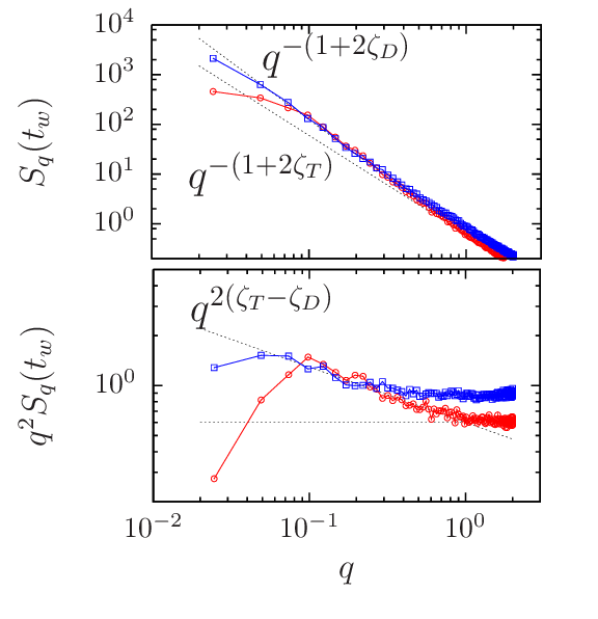
The thermal, , and disorder, , roughness exponents can also be extracted from the analysis of the structure factor defined in Eq. (5). Working with the structure factor is convenient since it is sufficient to simulate a long chain and then extract the dependence from the wave-vector dependence. Barabasi-Stanley Indeed, the roughness is simply related to the structure factor as
| (20) |
and this implies that the dynamic scaling (10)-(12) (for ) is equivalent to
| (21) |
with the equilibrium wave-vector dependent structure factor and for and for , with the internal dimension of the manifold ( for the directed line). These limits for the function ensure, respectively, the equilibrated steady geometry and the memory of the flat initial condition. In the case of power-law scaling Eq. (21) becomes
| (22) |
In the out of equilibrium relaxation process we are interested, depends on two-times and . The generalized scaling form then reads
| (23) |
that reduces to Eq. (21) both for , and to a similar form for for all , and thus stationarity is recovered. For fixed and we can study the dependence of on . If the aim is to determine the values of the roughness exponent the ideal choice would be to use a very long and plot for several ’s as a function of . This construction is to be compared with Fig. 2(b) in Ref. Sebastian, . In presence of disorder the construction should have a broken straight-line form with two exponents, ; the thermal one, , characterizing the behavior at short length-scales, , and the disorder one, , characterizing the behavior at long length-scales, . The breaking point defines a characteristic length which should depend on and we shall discuss and evaluate its precise temperature dependence in Sect. III.2.2. In an infinite -dimensional system disorder always dominates the fluctuations at very long length scales. However, in a finite system of length once all the system is characterized by thermal fluctuations and the value of is thus crucial.
Studying the wave-vector dependence of the structure factor is thus a convenient way to determine the roughness exponents, ; we hence expect to improve the values shown in Fig. 1(d) in Ref. EPL, . We studied the structure factor in the continuous disordered EW line. The general behavior described in the previous paragraphs is shown in Fig. 1 for working temperatures and . Note that the saturation of the structure factor at very small wave vector bears the same information as the fact that the roughness has not yet saturated at the longest time shown in Fig. 1. It means that the growing correlation length has not reached the size of the system, . The crossover from the thermal, , to the disorder, , roughness exponents is clear, with the expected values and confirmed. Note that the top panel in Fig. 1 shows the raw data while the bottom panel shows the structure factor multiplied by , which allows to better observe the crossover region and the difference between the two exponents.
III.2.2 The crossover length scale
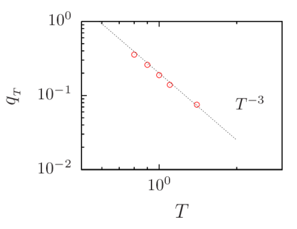
The analysis of the structure factor also allows us to evaluate the temperature and disorder strength dependence of the crossover length (or wave-vector ) and compare it to Yoshino’s unpublished results for the lattice model Yoshino-unp and Nattermann, Shapir and Vilfan’s estimate. Nattermann
The temperature-dependent crossover length separating the saturation regime characterized by the thermal and disorder exponents and should be observable in this presentation as a temperature-dependent crossover wave-vector in the equilibration prefactor . In order to access it one then needs to use a sufficiently long time-delay in such a way that the second factor saturates to .
The crossover length, and the crossover wave-vector, are expected to scale with temperature as , and , with an exponent that we shall obtain below using a variety of arguments. The characteristic length-scale should increase with increasing temperature (), indicating that thermal fluctuations become more and more important.
A simple argument to obtain the exponent relies on the fact that the fluctuations at large length scales () are not expected to strongly depend on the working temperature, in contrast with the short length scale ones. This is indeed confirmed in our numerical simulations, as can be observed comparing the two sets of data in Fig. 1. We will use this observation as a main input for the scaling argument in Sect. V. Let us assume that a weak temperature dependence is permitted, i.e. for , while for . Matching the crossover between these two regimes at one obtains
| (24) |
Using yields and . With simulations of the discrete model Yoshino found , Yoshino-unp in agreement with this result since for our one dimensional case .
A different prediction for the exponent comes from an order of magnitude argument. If one assumes that the characteristic free-energy barrier, , associated to the length-scale should be the thermal one,
| (25) |
one finds
| (26) |
If and are independent of temperature, and . Yoshino used this kind of argument with the free energy barrier replaced by the sample-to-sample fluctuations of the energy, an assumption tested in Ref. drossel, for low temperatures. In other words he replaced by , with the energy exponent to get ( in ). Yoshino-unp This argument assumes that the scale is the onset for thermally activated motion, making a connection between the dynamics and the geometry of the line.
On the other hand, using Flory-type arguments to predict the roughness exponent, for , with , and an expansion around , Nattermann et al Nattermann suggested and using they found in .
Figure 2 displays the result of the analysis of the crossover between the thermal and the disorder regimes in the structure factor at different working temperatures. Our numerical simulations of the disordered EW line is compatible with in agreement with the first two exposed arguments and Ref. Yoshino-unp, , see Eq. (24), but it rules out the value given by Nattermann et al. Nattermann However, by replacing the Flory approximation to the roughness exponent used by these authors by the exact exponent, we get again, in agreenment with our results.
III.2.3 The growing length: logarithmic growth from measurements
At high temperature, , equilibrium is quickly reached, disorder is irrelevant and one recovers stationary dynamics with the clean EW temperatue-independent values , and . At low temperature one has to distinguish between the thermal and disorder regimes and analyze the width of the crossover region.
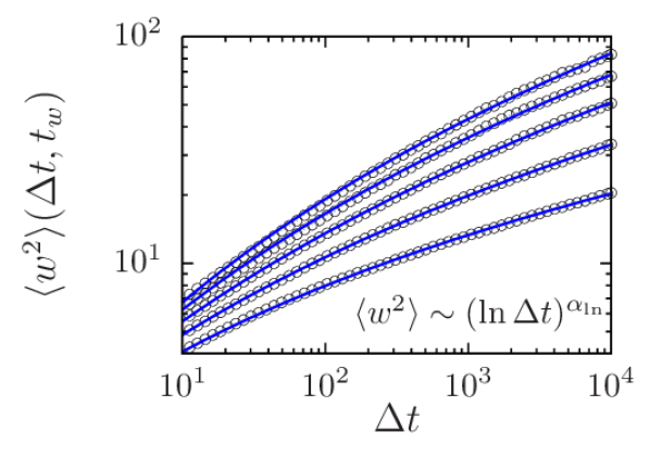
We shall first take and compare with the results obtained by Kolton et al Kolton (see also Ref. Yosh07, ). These authors showed, by studying the evolution of the structure factor of an elastic line in random media from a flat initial condition and using , that the characteristic growing length crosses over from a power-law dependence typical of the clean EW case to a logarithmic law, with (see Fig. 2 in Ref. Kolton, ). The exponent characterizes the scaling of the barriers at large scales, . Kolton et al expected , with the exponent characterizing the free-energy cost of an excitation of length , . The value of is known exactly for , , and the authors of Ref. Kolton, ascribed the discrepancy between the measured growing length, , and their expectation, to strong logarithmic corrections.
If the structure factor scales as in Eq. (21), the roughness scales as
| (27) |
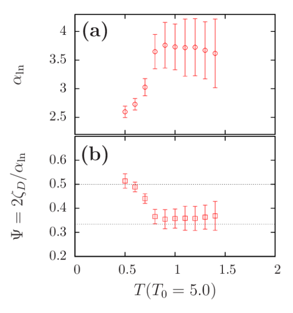
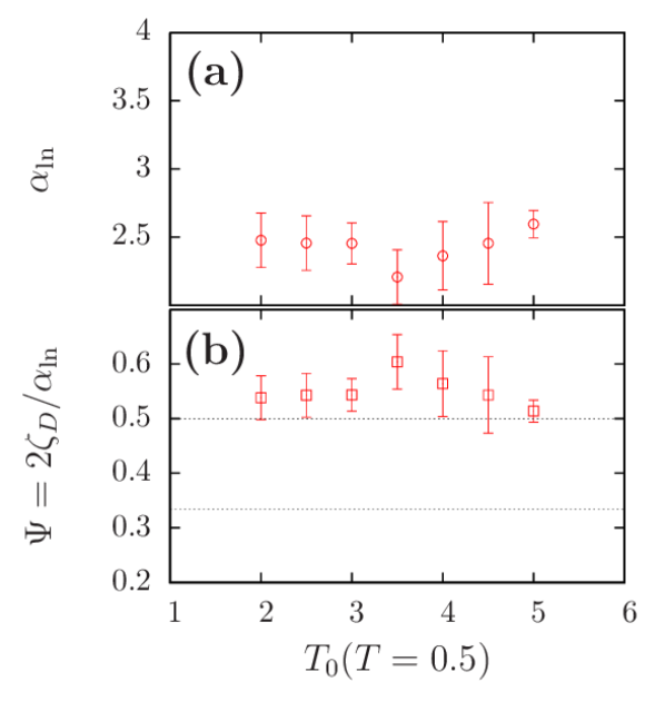
Using a long line, , as in Ref. Kolton, we confirm the logarithmic growth of the roughness for the case, as shown in Fig. 3. Different curves correspond to increasing temperatures, from bottom to top. We fit these curves to obtaining the temperature dependent exponent shown in Fig. 4(a). Now, by simply using the relation one recovers the exponent , i.e. , where we assumed that in this regime the disorder roughness exponent is the relevant one. We obtain which is close to the value obtained in Ref. Kolton, .
Recently, Monthus and Garel Monthus conjectured with the dimension of the surface of the excitation, in our case, that is in very good agreement with our numerical results at without any need to advocate for logarithmic corrections. However, the analysis at different working temperatures presented here reveals that the value of departs from and approaches for increasing temperature, see Fig. 4(b). This is the contrary to what is expected from the argument given in Ref. Monthus, that is based upon the role of the entropic contribution. Indeed, one would have expected the value to prevail at high temperatures, which is the opposite trend to what we find in the numerical simulations. We shall show in Sect. V that the temperature dependence of observed in Fig. 4(b) can be explained as a finite size/time effect induced by the crossover.
We have also analyzed the behavior of these exponents when changing the initial temperature, while keeping , that is to say, using initial conditions thermalized at different ’s. We performed the same fitting procedure keeping the working temperature fixed to and varying . The resulting exponents are shown in Fig. 5. Despite the rather large fluctuations we can trust that there is no systematic dependence on the initial temperature. We conclude that the exponent values do not depend on the previous history but they do on the relaxation conditions.
III.2.4 The growing length: pre-asymptotic power-law at finite
When the waiting time dependence is considered, the logarithmic growth is no longer easily observed. On the one hand, the crossover between the two asymptotic limits, and , makes it difficult to fit a logarithmic growth. On the other hand, when the correlation length increases the necessary time to reach the logarithmic regime increases exponentially . Thus, from a practical point of view, the logarithmic regime is not reached and one can use a power-law growth of the roughness as an effective description. We shall use such a power-law to analyze the aging behavior of the roughness in Sect. IV.1.
In this case, the best option to extract the dynamic growing length is to take a very long and study the breaking point in the structure factor. This breaking point separates the modes keeping the memory of the initial condition, , from the equilibrated modes described by the power-law regime with disorder exponent, . In the case of a power-law scaling, , one has
| (28) |
and from here one obtains . Using power-law fits we find that the growth and dynamic exponents, and , acquire a -dependence in the presence of quenched disorder Barrat ; Yoshino ; Yoshino-unp ; EPL while the roughness exponents do not depend on temperature.
IV Averaged aging dynamics
In this Section we analyze the two-time evolution of quantities that are averaged over many realizations of the thermal noise and quenched disorder. We consider two types of preparation: cooling from a higher temperature and heating from zero temperature. We discuss how the initial condition affects the behavior in the pre-asymptotic growth regime.
IV.1 The two-time roughness
The analysis of the averaged two-times roughness of a very long line described by the solid-on-solid model following a quench from infinite temperature was given in Refs. Barrat, ; Yoshino, ; Yoshino-unp, ; EPL, . We summarize here these results and we complement them by showing that: i. a similar scaling form describes the relaxation dynamics of the disordered EW line; ii. the dynamics after heating up the lines can also be described by the same scaling form with parameters that depend on the working and initial temperature; iii. the qualitative behavior is similar to the one found analytically for the clean EW Sebastian ; Pleimling and numerically for the clean KPZ Sebastian2 lines.
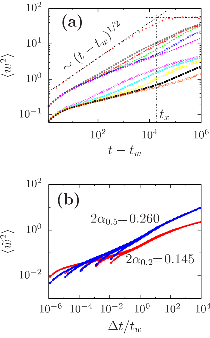
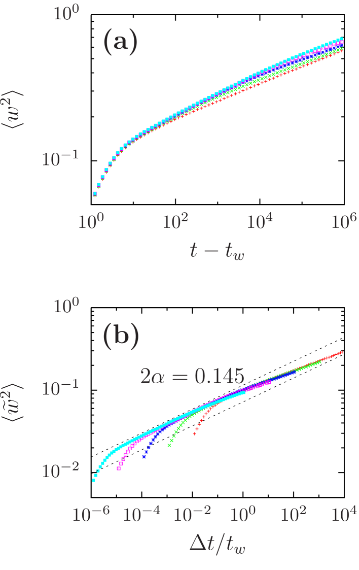
The time-difference dependence of the averaged roughness evolving from an infinite temperature initial condition in the SOS model, for several waiting-times and at three working temperatures, is shown in Fig. 6(a). The averaged roughness of the line evolving at high temperature, , is stationary. It grows as the clean EW roughness, and it reaches saturation at after . The line with evolving at is not stationary but signs of saturation are visible at MCs. The line evolving at low temperature, , shows aging effects, is still in the growth regime and does not reach saturation in the numerical time-window.
The averaged roughness curves in the growth regime can be well described by the scaling in Eq. (19). The numerical analysis of the growing length in the time-window we can reach indicates that . As discussed in Sect. III.2.3 this power-law regime should be considered as a pre-asymptotic approximation to a slower, logarithmic growth. We shall continue our analysis restricting to the power-law regime.
The resulting -dependent factor , see Eq. (19), can be well acquainted for by the empiric form EPL
| (29) | |||
Equations (19) and ((29) have the stationary limits:
| (32) |
with
| (33) |
These parameters control the two stationary asymptotes bounding the aging regime. The parameter is then a measure of the distance between the two asymptotes.
Figure 6(b) shows the scaling plot of the averaged roughness in the growth regime. We display data for at , and at . Note that the data for at shown in panel (a) of Fig. 6 would have not scaled properly since saturation appears earlier.
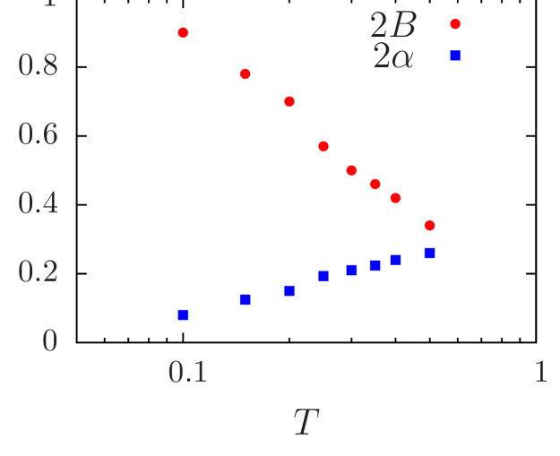
The temperature dependence of the (effective) growth exponent as well as the parameter for the solid-on-solid model evolving from an infinite temperature initial condition are shown in Fig. 7. The exponent approaches the EW value at high temperature. In the high-temperature limit the parameter approaches zero since the two constants and tend to the same temperature independent value and aging disappears.
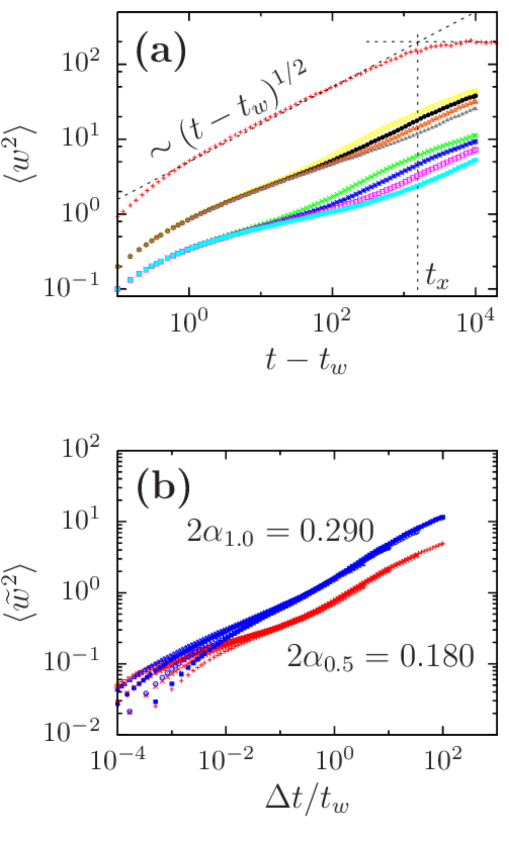
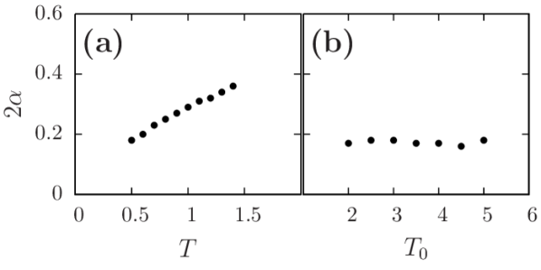
Figure 8 shows the averaged two-time roughness for the continuous model with a high initial temperature . The upper curve in Fig. 8(a) corresponds to the stationary case where the temperature is kept constant at the initial value. The other two cases, with and , present aging which is qualitatively similar to the SOS model of Fig. 6. Figure 8(b) shows the scaling of these curves with the temperature dependent exponents given in the key. In the continuous model the exponent increases with temperature until reaching the EW value after the crossover temperature . In Fig. 9(a) we present for the cases with a fixed initial temperature . As can be observed, its precise temperature dependence is not easy to determine. Since one expects that the exponent determines the slow dynamics at a given temperature, it is interesting to check that the value of at a small temperature does not depend on the initial temperature. This is shown in Fig. 9(b), where we show that is independent of the initial temperature. Although we do not compute the parameter for the continuous model, it is worth noting that in contrast with the discrete case the two constants and approach a temperature dependent asymptote that equals the high temperature limit of the EW line, and . Sebastian The exponent monotonically increases from and crosses over to at some with a very weak dependence.
The effect of using as an initial configuration one in equilibrium at a lower temperature was considered analytically in Ref. Sebastian, for the EW line. In presence of disorder one is often forced to use numerical simulations and the difficulty of equilibrating a long line at low temperature arises. However, a special case is that of the lattice model at . It is indeed well known that its ground state configuration can be exactly calculated by transfer-matrix methods. Kardar
In Fig. 10 we show the two-time roughness of the discrete disordered line using as initial configurations equilibrium ones at and a working temperature . The plots demonstrate that the trend of the curves is to reverse in the sense that the curves go from the upper to the lower asymptote. This behavior is similar to what was found analytically for the clean EW line Sebastian and the KPZ non-linear model. Sebastian2 This effect is also reminiscent of what was observed in the relaxation of the XY model from a uniform initial condition, corresponding to equilibrium at , at finite (higher) temperature within the spin-wave approximation. Behose
The effect of the initial condition can be summarized in the following way. At all working-temperatures that are identical to the one of the initial condition, , one finds and there is no aging since the line is initially in equilibrium. Sebastian For one has while for one has . The values of these constants determine the relative location of the two asymptotes of the growth regime, and .
IV.2 The linear response
We now turn to the study of the linear response. In Fig. 11 we show the averaged integrated linear response of the roughness in the lattice model. In panel (a) we show data for several waiting-times as a function of time delay. In panel (b) we scale the data as
| (34) |
with .
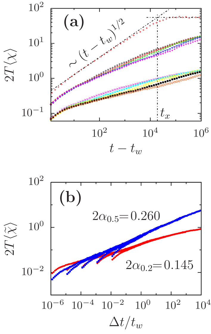
These results are to be confronted with the behavior of the EW elastic line with Langevin dynamics for which the integrated linear response is stationary and does not fluctuate. Sebastian On the other hand, the linear response obtained with the continuous model, not shown here, is qualitatively similar to the one shown for the SOS model in Fig. 11.
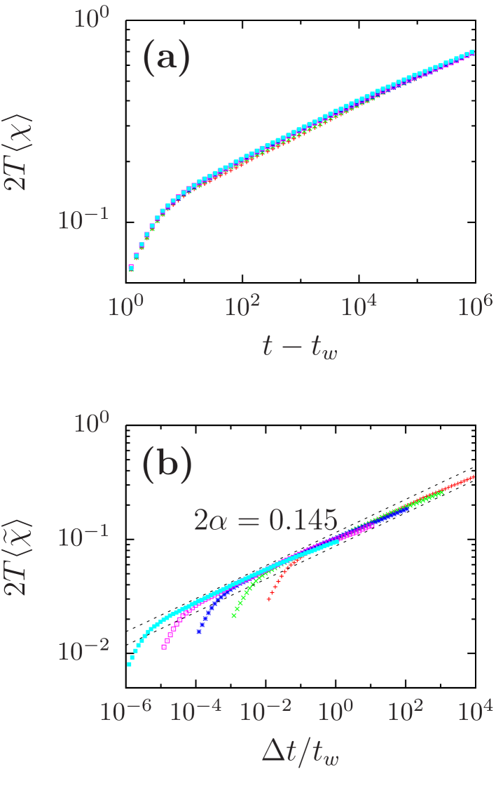
In Fig. 12 we display data for the linear response after the sudden heating from the ground state used in Sect. IV.1. The effect of this ‘reversed’ heating-procedure is similar to the one showed in Sect. IV.1 and in Fig. 10 for the roughness.
IV.3 The Fluctuation-dissipation theorem (FDT)
The modification of the FDT linking the displacement to its associated response in the lattice model after a quench from infinite temperature was studied by A. Barrat Barrat and Yoshino. Yoshino ; Yoshino-unp We here focus on the behavior of the roughness and its linear response. We show data for the disordered EW line after a similar quench. In Fig. 13 we show the plot against at fixed and using as a parameter going from to in the continuous disordered EW line for the case and . As it can be observed, it displays two slopes, allowing for the definition of an effective temperature Cukupe . A similar behaviour was reported for the displacement and associated linear response in the lattice model, Yoshino the clean EW line, Sebastian and the vortex glass model. us
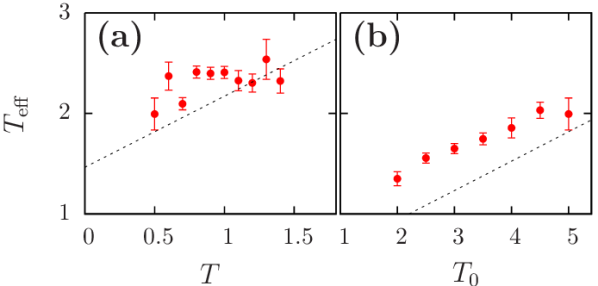
The temperature dependence of the effective temperature is shown in Fig. 14 for the disorder and the clean case. The dependence of on the working temperature while keeping fixed is shown in Fig. 14(a), but it is difficult to asses whether the effective temperature is constant or slowly grows with . Without disorder the EW solution gives a linear dependence , Sebastian shown with dashed lines in the figure. When the working temperature is fixed at and the initial temperature is changed, grows linearly with , as shown in Fig. 14(b) and in the clean limit.
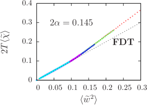
We also studied the effect of a heating procedure on the violations of the FDT using the lattice model. We show in Fig. 15 the parametric plot against using as initial condition the ground state at . As already found in the clean EW line we find that . thus reflects, consistently, a ‘memory’ of the initial configuration.
V Crossover-induced geometrical and dynamical effects
We discuss here how our numerical results can be explained by developing simple scaling arguments based on the existence of a single dynamic crossover in the growing correlation length at a static temperature dependent length , from a thermally dominated regime, to a disorder dominated regime with algebraically growing barriers as function of the length-scale. The main additional assumption on that we make is that at large enough length-scales , the geometry and typical barriers controlling the dynamics are indistinguishable from those at zero temperature. With these hypothesis, which are qualitatively supported by our numerical results, we can predict: (i) the temperature dependence of ; (ii) the temperature dependence of the effective exponents characterizing each regime of growth; (iii) the temperature dependence of the crossover time between these regimes; (iv) a parameter quantifying the importance of crossover-induced finite-size/time effects in simulations. In order to make the discussion in this Section self-contained we start by repeating some arguments that are well-known in the literature and then we present the scenario that, we propose, explains the numerical observations.
If the temperature is high enough to renormalize the microscopic pinning parameters, Nattermann thermal fluctuations dominate the line wandering at short length-scales. The geometry of equilibrated small scales, , is thus described by the thermal roughness exponent of the clean Edwards-Wilkinson (EW) equation, such that for or for , or . The typical time needed to equilibrate a length in this regime is therefore expected to be , with the EW dynamical exponent .
At length-scales , disorder dominates and the geometry of the equilibrated large length scales, , is the same as in the ground-state, for , with . The typical time to equilibrate a length is controlled by size-dependent energy barriers , such that , with . By hypothesis, we assume that both the form of and the barriers are independent of in this regime, in agreement with what is seen in Fig. 1 for the structure factor with .
In order to capture the crossover effects we interpolate the geometric and dynamic behavior of the regimes and described above. The static structure factor can be written as
| (35) |
with for and for . This interpolating form, which includes the temperature, is found to fit well the data, and to satisfy our assumption for . We continuously match the two regimes by requiring and, therefore,
| (36) |
with , which is the temperature dependence of the crossover length we observe in Fig. 2. This argument was also discussed in Sect. III.2.2 on numerical grounds, where references were also given.
Let us now discuss the dynamical behavior induced by . At the crossover we can roughly set , since barriers start to dominate the dynamics only above . For we expect . To interpolate the large scale behavior down to we use Nattermann
| (37) |
Since by hypothesis for , we obtain , with the energy exponent. The time to equilibrate a length can hence be written as
| (38) |
This expression continuously matches the barrier-dominated regime, for , with the power-law growth expected in the thermal regime, for . From Eq. (38) and using one obtains a characteristic time scale,
| (39) |
separating thermally from disorder dominated dynamics. This strong temperature dependence explains why the crossover to the slow logarithmic growth is particularly difficult to observe in numerical simulations. On the one hand, at high temperature, the line size must be large in order to see the crossover to the long-time logarithmic regime. On the other hand, at low temperature, the lines could in principle cross over to the logarithmic regime even for small system sizes but, because of the very slow Arrhenius activated dynamics, exceedingly long running times would be needed to resolve the precise time dependence. Most importantly, the data from any numerical simulation displaying the two regimes of growth will be characterized by temperature-dependent effective exponents due to crossover-induced finite-size/time effects, as we explain below.
Indeed, Eq. (38) allows us to explain the temperature dependence in the effective exponents of the power-law and logarithmic growth regimes. The influence of the crossover in the effective dynamical exponent of the power-law regime relevant to short length-scales, , follows from equating Eq. (38) to , which yields
| (40) |
To avoid solving the resulting self-consistent equation, we can use in the third member to obtain a first order correction to the dynamical exponent,
| (41) |
Since by construction the power-law fit of the data is done in a relatively short time-scale such that is almost constant (otherwise would not be well defined), and by using and , we get
| (42) |
This rough estimate is in good agreement with the numerically determined exponent shown in Figs. 7 and 9.
It is worth noting here that the Cardy-Ostlund random Sine-Gordon model Greg in , disordered ferromagnets, Pleimling-z and Ising and vector spin glasses Helmut were shown to display a dynamic exponent , with of the order of unity and depending on details of the considered model. Our arguments and numerical study show that the numerically measured dynamic exponent could simply be an effective value that stems from the interpolation of two growth regimes that cannot be properly resolved numerically. This seems to be particularly important for systems with a positive energy exponent , since in general we expect , and therefore a crossover from a thermally dominated short-time regime to a long-time dynamics dominated by diverging energetic barriers.
The temperature dependence of the effective exponent in the regime of logarithmic growth, , can be explained with a similar argument. By equating Eq. (38) to we find,
| (43) |
We use now and the time-dependence in the second member to get a self-consistent equation for , namely
| (44) |
Fixing the time scale and setting in the second member we obtain a first order approximation for ,
| (45) |
At high temperatures (or large times) such that this expression simply yields . In the opposite low limit for sufficiently large length scales such that the restriction is still satisfied one finds . Indeed, is a decreasing function of . These results are consistent with the result shown in Fig. 4, where we observe that at low temperatures, and increasing the temperature.
The effective exponent analysis made above reveals that crossover induced effects are controlled by the order of magnitude of . Since in a simulation is always a fraction of the system size , a temperature dependence of the effective exponents can be expected for systems such that . For instance, in order to properly resolve the dynamic exponent at short length scales we need for at least a few orders of magnitude range of , i.e. a large . On the other hand, to properly resolve the exponent we need for for at least a few orders of magnitude of . Typically, the largest systems analyzed numerically in the literature have , with and do not satisfy the latter constraint. This clearly prompts for a careful interpretation of the anomalous temperature dependence of power-law or logarithmic growth exponents obtained numerically so far, as we discuss below.
In Ref. Kolton, the relaxation of an elastic line in a disordered potential was analyzed for the particular case and . The crossover to the logarithmic growth was observed, though with an effective exponent . In Ref. Monthus, scaling arguments for the free energy of droplet excitations were given favoring the value , against the commonly accepted value , Kardar in apparent agreement with the results of Ref. Kolton, . In the present work we find for and , consistent with the result of Ref. Kolton, , but also a decrease towards a value close to with temperature. This behavior is opposite to what is proposed in Ref. Monthus, , where entropic effects leading to the value are expected to grow with , from the value , to the entropically-driven value . The scaling arguments given above thus show that the anomalous temperature dependence of can still be interpreted without dropping the identification, which was proposed time ago. Kardar
In numerical simulations of the steady-state slow driven motion of an elastic line Kolton-creep the effective creep exponent was found to be temperature dependent. According to the assumption at large length-scales, simple scaling arguments lead to (see, for instance Ref. giamarchi-kolton-rosso, ). Taking into account that in those simulations we can expect, following an equivalent line of reasoning as above, a temperature dependent effective creep exponent , such that when grows. This behavior is in good qualitative agreement with the results in Ref. Kolton-creep, . Therefore, the anomalous temperature dependence observed in Ref. Kolton-creep, can not be used as evidence against obtaining the creep exponent entirely as a function of static exponents, although the large scale geometry in the creep regime is found to be described by depinning exponents. Kolton-creep ; Kolton-vmcreep
VI Conclusions
Elastic manifolds are objects that appear in a large variety of problems with glassy features. It was shown in the past that these systems present aspects of glassy dynamics combined with diffusion properties. Cule ; Yoshino ; Barrat ; Yoshino-unp ; us ; EPL ; Sebastian ; Pleimling ; Sebastian2
After a series of analytic and numerical studies of continuous and discrete models with and without quenched disorder we can summarize the main features of the out of equilibrium relaxation of individual and interacting directed one-dimensional objects.
All these systems age below a characteristic temperature . In the mean-field limit of an infinite number of transverse dimensions, for a line with infinite length, a dynamic phase transition arise at . Below the lines age without diffusion. Cule
The dynamics of finite length lines moving in finite dimensional spaces cross over from diffusive-aging growth to a regime in which the roughness saturates. This phenomenon can be described with a generalization of the Family-Vicsek scaling. us ; Sebastian The qualitative features of the two-time freely relaxing observables are generic and do not depend on the presence of quenched randomness but the details such as the exponents and growing length do. We performed a careful analysis of the time-dependent growing length and we found a crossover from an effective power-law with temperature dependent exponent to the expected asymptotic logarithmic growth for sufficiently long strings. Our numerical data indicates a temperature dependent effective barrier exponent , which is higher than the energy exponent at low temperatures, but tends to it at high temperatures, provided the system is large enough to display the asymptotic behavior. As we discussed via scaling arguments this behavior can be recast in terms of crossover induced effects, and it is not inconsistent with the usual assumption for this system.
We also found a single crossover length separating a thermally dominated regime with and a disorder dominated regime with the roughness exponent . We showed that this is consistent with the assumption that large scale properties of the system are indistinguishable from those at . Translating this crossover into the dynamics we could also describe the temperature dependence of the effective dynamical exponents in the power-law growth regime, and in the logarithmic growth regime. In this respect it would be important to study the corresponding crossover in dimensions, relevant for vortices in superconductors. This is crucial for high-Tc superconductors where thermal fluctuations are known to strongly renormalize the disorder and produce Larkin lengths growing exponentially fast with temperature. rusos As the Larkin length marks the onset of metastability and the crossover to a barrier dominated (random-manifold) regime, as it does in our case, we can expect the phenomenology and crossover induced effects we describe here to be experimentally relevant, specially at the onset of irreversibility, near the transition to the vortex liquid phase, rusos ; us where the Larkin length can become comparable with the sample size. moira
The importance of measuring linear responses was demonstrated by the fact that all known coarsening systems (above their lower critical dimension) have an asymptotically vanishing linear response in the aging regime, in contrast to solvable mean-field glassy models and numerical simulations of finite dimensional glasses that yield a finite integrated linear response in the same two-times regime (see e.g. Refs. Leto, and Corberi, ). This fact appears as a concrete difference between the relaxation dynamics of coarsening and glassy systems.
The relaxation of the integrated thermal averaged linear response of elastic manifolds strongly depends on the presence or absence of quenched disorder. Mean-field elastic manifold models in quenched random environments have a fully aging linear response. The clean EW line has a stationary linear response while the dirty continuous or lattice models have integrated linear responses with aging and diffusion combined.
The effective temperature Cukupe defined from the comparison of induced and spontaneous averaged fluctuations is finite in all the cases considered as long as the diffusive factors in the correlations and linear responses are divided away. We also showed that the effective temperature is higher than the bath temperature for cooling procedures and, inversely, it is lower than the bath temperature for heating procedures. This is similar to what has been previously found in the XY model Behose and the Edwards-Wilkinson elastic line Sebastian and gives support to the notion of effectvie temperature as measured from deviations from the fluctuation-dissipation relation.
The study of dynamic fluctuations in these systems has not been fully developed yet. In Ref. EPL, we analyzed the fluctuations of the two-time roughness of the lattice disordered model during growth. The equilibrium Racz and out of equilibrium Sebastian roughness fluctuations in the EW line show a similar pattern. The probability distribution functions in all these models satisfy a scaling law and the scaling function follows the same trend as a function of all its variables. The question then arises as to whether the fluctuations of the linear responses of clean and disordered elastic lines are similar or different. We shall discuss this problem in a separate publication. The relation with the theory of fluctuations based on time-reparametrization invariance Chamon-Cugliandolo will also be discussed elsewhere.
Acknowledgments. We thank D. Domínguez, T. Giamarchi, G. Schehr and H. Yoshino for very useful discussions. LFC thanks the Universidad Nacional de Mar del Plata, Argentina; SB and JLI thank the Laboratoire de Physique Théorique et Hautes Energies, Université Pierre et Marie Curie Paris VI, for hospitality during the preparation of this work. SB also thanks the University of Genève and the DPMC, where part of this work was initiated and the Swiss NSF under MaNEP and Division II for support. The authors acknowledge financial support from ANPCyT-PICT20075, CONICET PIP5648 (JLI), and SECyT-ECOS P. A01E01/A08E03, and PICS 3172 (LFC). LFC is a member of Institut Universitaire de France.
References
- (1) A-L Barabási and H. E. Stanley, 1995 Fractal concepts in surface growth (Cambridge: Cambridge University Press); T. Halpin-Healey and Y-C Zhang, Phys. Rep. 254, 215 (1995).
- (2) A. J. Bray, Adv. Phys. 43, 357 (1994).
- (3) A. Hansen, E. L. Hinrichsen and S. Roux, Phys. Rev. Lett. 66, 2476 (1991); E. Bouchaud, J. Phys. Chem. 9, 4319 (1997); M. Alava, P. K. V. V. Nukalaz and S. Zapperi, Adv. Phys. 55, 349 (2006).
- (4) L. C. E. Struick, Physical aging in amorphous polymers and other materials (Elsevier, Amsterdam, 1978).
- (5) G. Blatter, M. V. Feigel’man, V. B. Geshkenbein, A. I. Larkin, and V. M. Vinokur, Rev. Mod. Phys. 66, 1125 (1994); T. Nattermann and S. Scheidl, Adv. Phys. 49, 607 (2000); T. Giamarchi and P. Le Doussal, in Spin glasses and random fields, A. P. Young ed. (World Scientific, Singapore, 1997).
- (6) S. Bustingorry, L. F. Cugliandolo and D. Domínguez, Phys. Rev. Lett. 96, 027001 (2006); S. Bustingorry, L. F. Cugliandolo, and D. Domínguez, Phys. Rev. B 75, 024506 (2007).
- (7) L. F. Cugliandolo, J. Kurchan, and L. Peliti, Phys. Rev. E 55, 3898 (1997).
- (8) L. F. Cugliandolo, in Slow Relaxations and Nonequilibrium Dynamics in Condensed Matter (Ecole de Physique Les Houches vol 77), ed J-L Barrat et al. (Berlin: Springer, 2003). Also available as [cond-mat/0210312].
- (9) F. Portier, G. Kriza, B. Sas, L. F. Kiss, I. Pethes, K. Vad, B. Keszei, and F. I. B. Williams, Phys. Rev. B 66, 140511(R) (2002); R. Exartier and L. F. Cugliandolo, Phys. Rev. B 66, 012517 (2002).
- (10) X. Du, G. Li, E. Y. Andrei, M. Greenblatt, and P. Shuk, Nature Phys. 3, 111 (2007).
- (11) L. F. Cugliandolo and P. Le Doussal, Phys. Rev. E 53, 1525 (1996); L. F. Cugliandolo, J. Kurchan, and P. Le Doussal, Phys. Rev. Lett. 76, 2390 (1996); Z. Konkoli, J. Hertz, and S. Franz, Phys. Rev. E 64, 051910 (2001); Z. Konkoli and J. Hertz, Phys. Rev. E 67, 051915 (2003); Y. Y. Goldschmidt, Phys. Rev. E 74, 021804 (2006).
- (12) A. Barrat, Phys. Rev. E 55, 5651 (1997).
- (13) H. Yoshino, J. Phys. A 29, 1421 (1996); Phys. Rev. Lett. 81, 1493 (1998).
- (14) H. Yoshino, unpublished.
- (15) S. Bustingorry, J. L. Iguain, C. Chamon, L. F. Cugliandolo, and D. Domínguez, Europhys. Lett. 76, 856 (2006).
- (16) F. Family and T. Vicsek, J. Phys. A 18, L75 (1985).
- (17) S. F. Edwards and D. R. Wilkinson, Proc. R. Soc. London Ser. A 381, 17 (1982).
- (18) S. Bustingorry, L. F. Cugliandolo, and J. L. Iguain, J. Stat. Mech. (2007) P09008.
- (19) A. Röthlein, F. Baumann, and M. Pleimling, Phys. Rev. E 74, 061604 (2006); Phys. Rev. E 76, 019901(E) (2007).
- (20) S. Bustingorry, J. Stat. Mech. (2007) P10002.
- (21) See also J. J. Ramasco, J. M. López and M. A. Rodríguez, Europhys. Lett. 76, 554 (2006).
- (22) M. Kardar, G. Parisi, and Y-C Zhang, Phys. Rev. Lett. 56, 889 (1986).
- (23) A. Rahmani, C. Castelnovo, J. Schmit, and C. Chamon, J. Stat. Mech. (2007) P09022.
- (24) D. Loi, S. Mossa, and L. F. Cugliandolo, Phys. Rev. E 77, 051111 (2008).
- (25) A. Rosso and W. Krauth, Phys. Rev. E 65, 025101(R) (2002).
- (26) T. Nattermann, Y. Shapir, and I. Vilfan, Phys. Rev. B 42, 8577 (1990).
- (27) A. B. Kolton, R. Exartier, L. F. Cugliandolo, D. Domínguez and N. Gronbech-Jensen, Phys. Rev. Lett. 89, 227001 (2002).
- (28) M. Kardar, Phys. Rev. Lett. 55, 2923 (1985); B. Drossel and M. Kardar, Phys. Rev. E 52, 4841 (1995).
- (29) B. Drossel and M. Kardar, Phys. Rev. E 52, 4841 (1995).
- (30) A. B. Kolton, A. Rosso, and T. Giamarchi, Phys. Rev. Lett. 95, 180604 (2005).
- (31) T. Nogawa, K. Nemoto, and H. Yoshino, Phys. Rev. B 77, 064204 (2008).
- (32) C. Monthus and T. Garel, J. Phys. A 41, 115002 (2008).
- (33) L. Berthier, P. W. C. Holdsworth, and M. Sellitto, J. Phys. A 34, 1805 (2001).
- (34) G. Schehr and P. Le Doussal, Phys. Rev. E 68, 046101 (2003); G. Schehr and P. Le Doussal, Phys. Rev. Lett. 93, 217201 (2004); G. Schehr and P. Le Doussal, Europhys. Lett. 71, 290 (2005); G. Schehr and H. Rieger, Phys. Rev. B 71, 184202 (2005).
- (35) M. Henkel and M. Pleimling, Europhys. Lett. 76, 561 (2006); M. Henkel and M. Pleimling, Phys. Rev. B 78, 224419 (2008).
- (36) H. G. Katzgraber and I. A. Campbell, Phys. Rev. B 72, 014462 (2005).
- (37) A. B. Kolton, A. Rosso, and T. Giamarchi, Phys. Rev. Lett. 94, 047002 (2005).
- (38) A. B. Kolton, A. Rosso, T. Giamarchi, and W. Krauth, Phys. Rev. Lett. 97 057001 (2006).
- (39) F. Corberi, E. Lippiello and M. Zannetti, J. Stat. Mech. (2004) P12007.
- (40) Z. Rácz, SPIE Proceedings 5112, 248 (2003).
- (41) C. Chamon and L. F. Cugliandolo, J. Stat. Mech. (2007) P07022.
- (42) D.S. Fisher and D.A. Huse, Phys. Rev. B 38, 386 (1988); Phys. Rev B 38, 373 (1988); Phys. Rev. B 43, 10728 (1991).
- (43) T. Giamarchi, A. B. Kolton, A. Rosso, Lecture Notes in Physics 688, 91 (2006).
- (44) M. I. Dolz, H. Pastoriza (private communication).