Pulsation modes in rapidly rotating stellar models based on the Self-Consistent Field method

Abstract

Context. New observational means such as the space missions CoRoT and Kepler and ground-based networks are and will be collecting stellar pulsation data with unprecedented accuracy. A significant fraction of the stars in which pulsations are observed are rotating rapidly.

Aims. Our aim is to characterise pulsation modes in rapidly rotating stellar models so as to be able to interpret asteroseismic data from such stars.

Methods. The pulsation code developed in Lignières et al. (2006) and Reese et al. (2006) is applied to stellar models based on the self-consistent field (SCF) method (Jackson et al. 2004, 2005, MacGregor et al. 2007).

Results. Pulsation modes in SCF models follow a similar behaviour to those in uniformly rotating polytropic models, provided that the rotation profile is not too differential. Pulsation modes fall into different categories, the three main ones being island, chaotic, and whispering gallery modes, which are rotating counterparts to modes with low, medium, and high $\ell-|m|$ values, respectively. The frequencies of the island modes follow an asymptotic pattern quite similar to what was found for polytropic models. Extending this asymptotic formula to higher azimuthal orders reveals more subtle behaviour as a function of $m$ and provides a first estimate of the average advection of pulsation modes by rotation. Further calculations based on a variational principle confirm this estimate and provide rotation kernels that could be used in inversion methods. When the rotation profile becomes highly differential, it becomes more and more difficult to find island and whispering gallery modes at low azimuthal orders. At high azimuthal orders, whispering gallery modes, and in some cases island modes, reappear.

Conclusions. The asymptotic formula found for frequencies of island modes can potentially serve as the basis of a mode identification scheme in rapidly rotating stars when the rotation profile is not too differential.

1 Introduction

New observational means are and will be collecting stellar pulsation data with unprecedented accuracy. The space mission CoRoT has considerably lowered the detection threshold for pulsation modes, thus allowing photometric observation of solar-like pulsations in stars other than the Sun and increasing the number of detected modes in early-type stars. The forthcoming space mission Kepler will add a wealth of pulsation data by observing a large number of stars for a period of four years. Other projects include the space mission PLATO as well as ground-based networks such as SONG.

Stellar pulsations yield valuable information on the internal structure of stars which can be used to constrain stellar evolution models. Although a great deal of success has been achieved in probing the internal structure of the Sun and of a number of other stars, a number of difficulties arise for rapidly rotating stars. Indeed, rapid stellar rotation introduces a number of phenomena which considerably complicate their modelling and the study of their pulsation modes. These include centrifugal deformation, gravity darkening, baroclinic flows and various forms of turbulence and transport phenomena (e.g.  Rieutord 2006b). As a result, the internal structure of these stars remain difficult to probe.

Traditionally, the effects of rotation on pulsation modes have been modelled using the perturbative approach. In this approach, rotation is taken into account through corrections which are added to the non-rotating solutions. The underlying assumption in this method is that the rotation rate, $\Omega$, can be treated as a small parameter, thus enabling one to develop the perturbative corrections as a power series in $\Omega$. Such series can be extended to first (Cowling & Newing 1949, Ledoux 1951), second (Saio 1981, Gough & Thompson 1990, Dziembowski & Goode 1992) or third order in $\Omega$ (Soufi et al. 1998, Karami et al. 2005). A natural question to ask is up to what rotation rate is this approach valid. This remained an open question until Reese et al. (2006) applied a non-perturbative two-dimensional approach to calculating acoustic pulsations in polytropic stellar models and compared the results with perturbative calculations. Their results showed that perturbative methods remain valid only for values which are lower than the rotation rate of many early-type stars. Further comparisons between the two approaches include those by Lovekin & Deupree (2008), in which more realistic models were used but at a lower accuracy, and Ouazzani et al. (2009), in which the effects of avoided crossings are included in the perturbative calculations.

Due to the limitations of the perturbative method, a number of recent studies have focused on modelling the effects of rapid rotation on stellar acoustic pulsations using a two-dimensional approach. Espinosa et al. (2004) studied the effects of rapid rotation on frequency multiplets in models with a uniform density and also briefly discussed pulsations of realistic models. They showed how rotation leads to highly non-uniform multiplets and causes the frequencies of adjacent modes to pair up, thus providing a tentative explanation for observed close frequency pairs (Breger & Pamyatnykh 2006). Lignières et al. (2001) studied pulsation modes in a uniform density spheroid using a perturbative method and two different numerical approaches. This was done in order to validate their two-dimensional numerical method before applying it to more realistic models. Their work was followed by Lignières et al. (2006), Reese et al. (2006) and Reese et al. (2008a) who did the first accurate calculations of p-modes in rapidly rotating polytropic models. They investigated the limits of the perturbative approach, studied disk averaging factors which intervene in mode visibility, compared the effects of the centrifugal and Coriolis forces and found an empirical formula which characterises the structure of the frequency spectrum for low degree modes. At the same time, Lignières & Georgeot (2008) and Lignieres & Georgeot (2009) applied ray dynamics to the study of acoustic modes in rotating polytropic models. They classified modes into several categories, the main ones being island, chaotic, and whispering gallery modes which are rotating counterparts to modes with low, intermediate, and high $\ell-|m|$ values, where $\ell$ is the harmonic degree and $m$ the azimuthal order. They showed that each category has its own frequency organisation and provided an explanation involving travel time integrals for the empirical formula found in Lignières et al. (2006) and Reese et al. (2008a). Finally, Lovekin & Deupree (2008) and Lovekin et al. (2009) studied p-modes with low radial orders in realistic models from Deupree (1990) and Deupree (1995) with both uniform and differential rotation. They investigated how frequencies and the large and small separations vary with uniform or differential rotation and compared their calculations with a perturbative approach.

Before being able to interpret pulsation modes in observed stars, more progress is needed in understanding the effects of rotation on pulsation modes. Indeed, although a number of important results have been established for p-modes in polytropic models, these need to be extended to more realistic models. The calculations involving more realistic models have currently been limited to small mode sets and the analysis has not been pushed far enough to see whether similar results apply. In what follows, we calculate pulsation modes, using the numerical method developed in Lignières et al. (2006) and Reese et al. (2006), in realistic models of rapidly rotating stars based on the Self-Consistent Field (SCF) method (Jackson et al. 2005, MacGregor et al. 2007). In particular, we investigate whether a similar mode classification exists in these models, whether a similar empirical formula applies to frequencies of modes with low $\ell-|m|$ values, and quantify the effects of using a differential profile. The next section deals with the SCF method and the models it produces. The following section explains the pulsation equations, the numerical method used for calculating the pulsation modes and a number of tests to validate the method. Afterwards, Sections 3 and 4 describe the results for models with mildly and strongly differential rotation, respectively. Our conclusions are summarised in Section 5.

2 Stellar models based on the SCF method

The SCF method is an iterative procedure for solving the equations that govern the structure of a conservatively rotating star. The basic approach underlying the method is to alternately solve Poisson’s equation to derive the 2D shapes of equipotential surfaces, and the equations of mass, momentum, and energy conservation to obtain the 1D profiles of thermodynamic quantities along a radius in the rotational equatorial plane. As described in detail in Jackson et al. (2005), this procedure yields a sequence of models which, under most circumstances, converges to a model that satisfies all the equations for a prescribed internal rotation law.

The method was first developed and used 40 years ago to compute uniformly and differentially rotating polytropic stellar models (Ostriker & Mark 1968). Although subsequently extended through the incorporation of more realistic input physics (Jackson 1970), application of the method was limited to massive stars, a consequence of convergence difficulties encountered in lower mass models with sufficiently high values of the central mass concentration (see, e.g., Clement 1978). This problem was addressed and remedied through a reformulation of the method in which the normalised distributions of thermodynamic quantities and the central values of those quantities are adjusted in separate iterative loops. The new SCF method has been implemented in a code that utilises up-to-date input physics. The opacities are obtained from the tables of OPAL opacities computed by Rogers & Iglesias (1992) and from tables of low-temperature opacities compiled by Alexander & Ferguson (1994), using interpolation subroutines written by Vandenberg (1983). The equation of state for the stellar material is calculated according to the formula of Eggleton et al. (1973), and the nuclear energy generation rates for hydrogen burning are from Caughlin & Fowler (1988), with the treatment of electron screening effects from Graboske et al. (1973) for the case of equilibrium abundances of CNO isotopes. Energy transport in sub-photospheric convective envelopes is treated using a standard mixing-length model (see, e.g., Kippenhahn et al. 1967), in which the local gravitational acceleration $\@vec{g}$ is replaced by the value of $\@vec{g}$ as reduced by the local centrifugal acceleration, averaged over equipotential surfaces. For the models utilised in the pulsation mode computations described in subsequent sections, a value of 1.9 was adopted for the ratio of the mixing length to the pressure scale height. The method and the code are both robust and rapidly convergent, and have been thoroughly tested and validated through such applications as the interpretation of interferometric observations of rapid rotators like the Be star Achernar (Jackson et al. 2004, and references therein) and an examination of the effects of differential rotation on the structure of stars less massive than 2 $M_{\odot}$ (MacGregor et al. 2007).

Models computed using the SCF method are chemically homogeneous, ZAMS models with the following abundance fractions by weight of H, He, and heavy elements: $X=0.7112$, $Y=0.27$, and $Z=0.0188$. The rotation profile is imposed beforehand and is conservative, i.e. the centrifugal force derives from a potential. As a result, the stellar structure is barotropic – different thermodynamic quantities remain constant along lines of constant total (centrifugal plus gravitational) potential. The rotation profile used in the present calculations was:

$$\Omega(s)=\frac{\eta\Omega_{\mathrm{cr}}}{1+\left(\frac{\alpha s}{R_{\mathrm{eq}}}\right)2}$$ (1)

where $s$ is the distance from the rotation axis, $R_{\mathrm{eq}}$ the equatorial radius, and $\Omega_{cr}$ the break-up rotation rate at $R_{\mathrm{eq}}$. The parameters $\eta$ and $\alpha$ determine how rapid and differential the rotation is. In particular, the ratio between the polar and equatorial rotation rate is $1+\alpha^{2}$. The associated angular momentum increases with $s$ thereby satisfying the dynamical part of the Solberg-Høiland criterion for stability. Various forms of shear instability may, however, be present if the rotation profile becomes too differential, i.e. if $\alpha$ becomes too large (e.g.  Zahn 1974). Also, as explained in Zahn (1993) and Rieutord (2006a), baroclinic flows occur in radiative zones of rapidly rotating stars thus leading to a non-conservative rotation profile. Exploring these effects is, however, beyond the scope of this paper.

Equation (1) corresponds to a rotation profile in which the rotation rate decreases with $s$. Such profiles can be used to construct highly distorted configurations. Indeed, the stellar core can be made to rotate quite rapidly since the local break-up velocity is larger than at the equator. This type of model was used to try to explain Achernar’s extreme oblateness (Jackson et al. 2004). The SCF method can also produce models with a rotation rate that increases with distance from the rotation axis. This resembles somewhat the solar rotation profile in which the rotation rate increases with decreasing latitude in the convection zone (Schou et al. 1998, Thompson et al. 2003).

2.1 The pulsation equations

In order to derive the set of equations which govern acoustic pulsation modes in a differentially rotating star, we start by representing the differential rotation by a permanent background flow $\@vec{v}_{o}=s\Omega(s)\@vec{e}_{\phi}$. In what follows, we will work with cylindrical coordinates $(s,z,\phi)$ and their associated unit vectors $(\@vec{e}_{s},\@vec{e}_{z},\@vec{e}_{\phi})$. We write out the Eulerian perturbation to various equations, starting with Euler’s equation, and only keep first order linear terms:

$$\rho_{o}\frac{\partial\@vec{v}}{\partial t}+\rho\@vec{v}_{o}\cdot\@vec{\nabla}\@vec{v}_{o}+\rho_{o}\@vec{v}\cdot\@vec{\nabla}\@vec{v}_{o}+\rho_{o}\@vec{v}_{o}\cdot\@vec{\nabla}\@vec{v}=-\@vec{\nabla}p+\rho\@vec{g}_{\mathrm{o}}-\rho_{o}\@vec{\nabla}\Psi,$$ (2)

where quantities with the subscript “$o$” are equilibrium quantities, and those without a subscript Eulerian perturbations. The quantity $\@vec{g}_{\mathrm{o}}$ is the background gravity excluding the centrifugal acceleration. The different terms on the left hand side of Eq. (2) can be worked out explicitly in terms of $\Omega(s)$:

$$\@vec{v}_{o}\cdot\@vec{\nabla}\@vec{v}_{o} = -s\Omega^{2}\@vec{e}_{s},$$ (3)

$$\@vec{v}\cdot\@vec{\nabla}\@vec{v}_{o} = \@vec{\Omega}\times\@vec{v}+v_{s}s\partial_{s}\Omega\@vec{e}_{\phi},$$ (4)

$$\@vec{v}_{o}\cdot\@vec{\nabla}\@vec{v} = \@vec{\Omega}\times\@vec{v}+im\Omega\@vec{v},$$ (5)

where we have assumed an $e^{im\phi}$ azimuthal dependence for $\@vec{v}$ and $\@vec{\Omega}=\Omega\@vec{e}_{z}$. The first term corresponds to the centrifugal acceleration and the sum of the next two includes the Coriolis force. Combining these equations with Eq. (2) yields:

$$\left[\lambda+im\Omega\right]\rho_{o}\@vec{v}=-\@vec{\nabla}p+\rho\@vec{g}_{\mathrm{eff}}-\rho_{o}\@vec{\nabla}\Psi-2\@vec{\Omega}\times\rho_{o}\@vec{v}-\rho_{o}s\frac{\partial\Omega}{\partial s}v_{s}\@vec{e}_{\phi}.$$ (6)

where we have assumed an $e^{\lambda t}$ time dependence for $\@vec{v}$ and where $\@vec{g}_{\mathrm{eff}}=\@vec{\nabla}p_{o}/\rho_{o}$ is the background effective gravity which includes the centrifugal acceleration. The Eulerian perturbation to the continuity equation gives:

$$\frac{\partial\rho}{\partial t}+\@vec{\nabla}\cdot\left(\rho_{o}\@vec{v}\right)+\@vec{\nabla}\cdot\left(\rho\@vec{v}_{o}\right)=0.$$ (7)

In terms of $\Omega$, this becomes:

$$\left[\lambda+im\Omega\right]\rho=-\@vec{v}\cdot\@vec{\nabla}\rho_{o}-\rho_{o}\@vec{\nabla}\cdot\@vec{v}.$$ (8)

The Eulerian perturbation to Poisson’s equation is simply:

$$\Delta\Psi=4\pi G\rho,$$ (9)

where $G$ is the gravitational constant. These equations are then supplemented by the adiabatic relation between the pressure and density perturbations which takes on the following form:

$$\frac{\partial p}{\partial t}+\@vec{v}\cdot\@vec{\nabla}p_{o}+\@vec{v}_{o}\cdot\@vec{\nabla}p=c_{o}^{2}\left[\frac{\partial\rho}{\partial t}+\@vec{v}\cdot\@vec{\nabla}\rho_{o}+\@vec{v}_{o}\cdot\@vec{\nabla}\rho\right]$$ (10)

where $c_{o}^{2}=\frac{\Gamma_{1}p_{o}}{\rho_{o}}$ is the square of the sound velocity and $\Gamma_{1}$ the adiabatic exponent. Provided that $\@vec{v}_{o}\cdot\@vec{\nabla}p_{o}=\@vec{v}_{o}\cdot\@vec{\nabla}\rho_{o}=\@vec{v}_{o}\cdot\@vec{\nabla}c_{o}^{2}=0$, this form can be shown to be equivalent to $\delta p=c_{o}^{2}\delta\rho$ where $\delta p$ and $\delta\rho$ are the Lagrangian pressure and density perturbations, respectively. This leads to the following equation after some manipulations:

$$\left[\lambda+im\Omega\right]\left(p-c_{o}^{2}\rho\right)=\left[-\@vec{\nabla}p_{o}+c_{o}^{2}\@vec{\nabla}\rho_{o}\right]\cdot\@vec{v}\\$$ (11)

2.2 Non-dimensional form

These equations are then put into non-dimensional form using the following length, density and pressure scale factors:

$$R_{\mathrm{eq}},\qquad p_{c},\qquad\rho_{c},$$ (12)

where the subscript “$c$” refers to the centre of the star, and $R_{\mathrm{eq}}$ is the equatorial radius. This gives a time scale $t_{\mathrm{ref}}$ defined as:

$$t_{\mathrm{ref}}=\left(\frac{\rho_{c}R_{\mathrm{eq}}^{2}}{p_{c}}\right)^{1/2}$$ (13)

Based on these scale factors, all of the above equations remain the same as in dimensional form, except for Poisson’s equation where a non-dimensional factor $\Lambda=4\pi G\rho_{c}^{2}R_{\mathrm{eq}}^{2}/p_{c}$ appears:

$$\Delta\Psi=\Lambda\rho.$$ (14)

2.3 Spheroidal geometry

In order to achieve higher accuracy when solving these equations numerically, a coordinate system which follows the shape of the star is introduced. This new coordinate system $(\zeta,\theta,\phi)$ can be related to the usual spherical coordinate system $(r,\theta,\phi)$ via the following relationship:

$$r(\zeta,\theta)=(1-\varepsilon)\zeta+\frac{5\zeta^{3}-3\zeta^{5}}{2}\left(R_{s}(\theta)-1+\varepsilon\right),$$ (15)

for $\zeta\in[0,1]$. When $\zeta=1$, $r$ coincides with the stellar surface, $R_{s}(\theta)$. The variables $\theta$ and $\phi$ remain the same in both systems. A second domain is added around the first, in which $r$ is given by:

$$r(\zeta,\theta)=2\varepsilon+(1-\varepsilon)\zeta+\left(2\zeta^{3}-9\zeta^{2}+12\zeta-4\right)\left(R_{s}(\theta)-1-\varepsilon\right),$$ (16)

for $\zeta\in[1,2]$. With these definitions, $r$ and $r_{\zeta}\equiv\partial_{\zeta}r$ remain continuous across $\zeta=1$. As $\zeta$ approaches $0$ or $2$, this coordinate system behaves like a spherical coordinate system: the constant $\zeta$-lines become spherical and $r_{\zeta}$ becomes independent of $\theta$. This is important as it simplifies the regularity conditions in the centre and the boundary condition on the perturbation to the gravity potential on the outer boundary. The same coordinate system was used in Lignières et al. (2006) and Reese et al. (2006) and is based on Bonazzola et al. (1998). The stellar model is then interpolated onto a grid based on this new coordinate system.

Another possibility would be to base the radial coordinate on the equipotentials. This has the advantage of simplifying the pulsation equations because terms such as $\partial_{\theta}\rho_{o}$ and $\partial_{\theta}p_{o}$ vanish. However, this requires using numerical rather than analytical differentiation when calculating terms with radial derivatives such as $r_{\zeta}$, thereby reducing the accuracy of the results. Furthermore, the regularity conditions in the centre of the star become more complicated as the equipotentials do not in general become circular towards the centre.

Based on the coordinate system presented above, the continuity equation becomes:

$$\left[\lambda+im\Omega\right]\rho=-\frac{\zeta^{2}\partial_{\zeta}\rho_{o}}{r^{2}r_{\zeta}}u^{\zeta}-\frac{\zeta\partial_{\theta}\rho_{o}}{r^{2}r_{\zeta}}u^{\theta}-\frac{\zeta^{2}\rho_{o}}{r^{2}r_{\zeta}}\left[\frac{\partial_{\zeta}\left(\zeta^{2}u^{\zeta}\right)}{\zeta^{2}}+\frac{\partial_{\theta}\left(\sin\theta u^{\theta}\right)}{\zeta\sin\theta}+\frac{\partial_{\phi}u^{\phi}}{\zeta\sin\theta}\right],\\$$ (17)

Euler’s equation takes on the following form:

$$\left[\lambda+im\Omega\right]\rho_{o}\left[\frac{\zeta^{2}r_{\zeta}u^{\zeta}}{r^{2}}+\frac{\zeta r_{\theta}u^{\theta}}{r^{2}}\right] = \rho_{o}\frac{2\Omega\zeta\sin\theta u^{\phi}}{r}-\partial_{\zeta}p+\frac{\partial_{\zeta}p_{o}}{\rho_{o}}\rho-\rho_{o}\partial_{\zeta}\Psi,$$ (18)

$$\left[\lambda+im\Omega\right]\rho_{o}\left[\frac{\zeta^{2}r_{\theta}u^{\zeta}}{r^{2}}+\frac{\zeta(r^{2}+r_{\theta}^{2})u^{\theta}}{r^{2}r_{\zeta}}\right] = \rho_{o}\frac{2\Omega\zeta(r_{\theta}\sin\theta+r\cos\theta)u^{\phi}}{rr_{\zeta}}-\partial_{\theta}p+\frac{\partial_{\theta}p_{o}}{\rho_{o}}\rho-\rho_{o}\partial_{\theta}\Psi,$$ (19)

$$\left[\lambda+im\Omega\right]\rho_{o}\frac{\zeta u^{\phi}}{r_{\zeta}} = -\rho_{o}\frac{2\Omega\zeta^{2}\sin\theta u^{\zeta}}{r}-\rho_{o}\frac{2\Omega\zeta(r_{\theta}\sin\theta+r\cos\theta)u^{\theta}}{rr_{\zeta}}-\frac{\partial_{\phi}p}{\sin\theta}$$ (20)

$$-\rho_{o}\frac{\partial_{\phi}\Psi}{\sin\theta}-\rho_{o}\sin\theta\left(\partial_{s}\Omega\right)\left[\zeta^{2}\sin\theta u^{\zeta}+\frac{\zeta(r_{\theta}\sin\theta+r\cos\theta)}{r_{\zeta}}u^{\theta}\right],$$

the adiabatic relation is given by:

$$\left[\lambda+im\Omega\right]\left(p-c_{o}^{2}\rho\right)=\frac{\zeta^{2}}{r^{2}r_{\zeta}}\left(-\partial_{\zeta}p_{o}+c_{o}^{2}\partial_{\zeta}\rho_{o}\right)u^{\zeta}+\frac{\zeta}{r^{2}r_{\zeta}}\left(-\partial_{\theta}p_{o}+c_{o}^{2}\partial_{\theta}\rho_{o}\right)u^{\theta},\\$$ (21)

and Poisson’s equation takes on the following form:

$$0=\frac{r^{2}+r_{\theta}^{2}}{r^{2}r_{\zeta}^{2}}\partial^{2}_{\zeta\zeta}\Psi+c_{\zeta}\partial_{\zeta}\Psi-\frac{2r_{\theta}}{r^{2}r_{\zeta}}\partial^{2}_{\zeta\theta}\Psi+\frac{1}{r^{2}}\Delta_{\theta\phi}\Psi-\Lambda\rho,$$ (22)

where $u^{\zeta}$, $u^{\theta}$, and $u^{\phi}$ are the three velocity components (see below for details) and terms of the form $r_{\zeta}$, $r_{\theta}$ … are different derivatives of $r$ based on Eqs. (15) and (16). Explicit expression for $c_{\zeta}$ and $\Delta_{\theta\phi}$ are as follows:

$$c_{\zeta} = \frac{1}{r^{2}r_{\zeta}^{3}}\left(2r_{\zeta}r_{\theta}r_{\zeta\theta}-r^{2}r_{\zeta\zeta}-r_{\zeta}^{2}r_{\theta\theta}+2rr_{\zeta}^{2}-r_{\theta}^{2}r_{\zeta\zeta}-r_{\zeta}^{2}r_{\theta}\cot\theta\right),$$ (23)

$$\Delta_{\theta\phi} = \partial^{2}_{\theta\theta}+\cot\theta\partial_{\theta}+\frac{1}{\sin^{2}\theta}\partial^{2}_{\phi\phi}.$$ (24)

The above expressions are obtained by using tensorial expressions for the differential operators which intervene and working them out explicitly. Furthermore, the components to the velocity are written on the following basis:

$$\begin{array}[]{lllll}\@vec{a}_{\zeta}&=&\displaystyle\frac{\zeta^{2}}{r^{2}r_{\zeta}}\@vec{E}_{\zeta}&=&\displaystyle\frac{\zeta^{2}}{r^{2}}\@vec{e}_{r},\\ \@vec{a}_{\theta}&=&\displaystyle\frac{\zeta}{r^{2}r_{\zeta}}\@vec{E}_{\theta}&=&\displaystyle\frac{\zeta}{r^{2}r_{\zeta}}\left(r_{\theta}\@vec{e}_{r}+r\@vec{e}_{\theta}\right),\\ \@vec{a}_{\phi}&=&\displaystyle\frac{\zeta}{r^{2}r_{\zeta}\sin\theta}\@vec{E}_{\phi}&=&\displaystyle\frac{\zeta}{rr_{\zeta}}\@vec{e}_{\phi},\end{array}$$ (25)

where $\left\{\@vec{E}_{i}\right\}$ and $\left\{\@vec{e}_{i}\right\}$ are the natural and spherical basis, respectively. When the star becomes spherical, the basis $\left\{\@vec{a}_{i}\right\}$ converges to $\left\{\@vec{e}_{i}\right\}$. Apart from some multiplicative factors, Euler’s equation is expressed on the dual basis, as is done in Reese et al. (2006), since this has the advantage of limiting the effective gravity to the radial component at the stellar surface. More details on how to derive the above expressions can be found in Reese (2006) and references therein.

Equations (17)-(22) were completed with a number of boundary conditions which ensure that the solution remains regular in the centre, the Lagrangian pressure perturbation vanishes on the stellar surface and the perturbation to the gravitational potential goes to zero at an infinite distance from the star.

2.4 Numerics

The above equations were then projected onto the spherical harmonic basis in the same way as was done in Lignières et al. (2006) and Reese et al. (2006). This is achieved by expressing the different unknowns as a sum of scalar or vectorial spherical harmonics multiplied by unknown radial functions, and then projecting the equations themselves onto the spherical harmonic basis, using Gaussian quadrature to numerically perform the integrations. The resultant system is an infinite system of coupled ordinary differential equations in terms of the radial variable $\zeta$ which is truncated at a maximal harmonic degree $L_{\mathrm{max}}$. The solution to this system yields the radial functions used in the harmonic decomposition of the different unknowns.

This system of ordinary differential equations is discretised using one of three methods: a spectral method based on Chebyshev polynomials, finite differences or a polynomial spline-based method. In the latter two cases, the order can be adjusted. When applying these methods, the stellar model is interpolated onto either a higher resolution uniform grid or a Chebyshev Gauss-Lobatto collocation grid using cubic spline interpolation. For the spectral method, this is analogous to what was done in Dintrans & Rieutord (2000) in which a $1.5\,\,M_{\odot}$ CESAM model was interpolated onto the same type of collocation grid before being used to calculate gravito-inertial modes.

After discretisation, the eigenvalue problem is in algebraic form: $\mathcal{A}v=\lambda\mathcal{B}v$ where $\mathcal{A}$ and $\mathcal{B}$ are square matrices. With a suitable choice of variables, these matrices can be made real, thereby reducing the computational cost. Also, pulsation modes are either symmetric or anti-symmetric with respect to the equator, so that only spherical harmonics of the same parity are needed to describe them. The problem is then solved numerically using the Arnoldi-Chebyshev algorithm (e.g.  Chatelin 1988) around different target frequencies, called frequency shifts. In what follows, most of the calculations have been done using a 4^th order finite difference approach. The angular resolution was typically $L_{\mathrm{max}}=80$ and the radial resolution $N_{\mathrm{r}}=501$.

2.5 Accuracy of the calculations

Various tests can be used to assess the accuracy of the calculations. A first test consists in following the evolution of the frequency error as a function of the radial and angular resolution. The solid lines in Fig. 1 show the evolution of the relative error on the numerical frequency for two modes in a $25$ $M_{\odot}$ model uniformly rotating at $60\%$ of the break-up rotation rate, using the frequencies calculated at highest resolution as references. The first two panels apply to an $\tilde{n}=16$ mode and the other two to $\tilde{n}=50$ (see Section 3 for the definition of $\tilde{n}$). As is evident from the figure, the stability of the numerical frequencies is very good, especially for the angular resolution where spectral convergence seems to be achieved.

Intermediate radial order	High radial order

Figure 1: Evolution of various forms of the frequency error with $L_{\mathrm{max}}$ and $N_{\mathrm{r}}$ for two pulsation modes in an 25 $M_{\odot}$ star rotating uniformly at $60\%$ of the break-up velocity. The mode on the left corresponds to $\tilde{n}=16$ and the one the right to $\tilde{n}=50$ (the meaning of $\tilde{n}$ is given in Section 3 and illustrated in Fig. 3). The solid and dotted lines correspond to the relative frequency error. This first case uses the numerical frequency and the second is based on the variational frequency. The dashed curve shows the relative difference between the numerical and variational frequencies. The frequencies $\Omega_{o}$ and $\Omega_{o}^{\mathrm{var}}$ are the numerical and variational frequencies calculated at highest resolution (i.e. $L_{\mathrm{max}}=100$, $N_{\mathrm{r}}=751$ for the mode on the left and $L_{\mathrm{max}}=160$, $N_{\mathrm{r}}=1001$ for the mode on the right). As can be seen in the figures, the numerical frequencies are very stable as a function of the resolutions, and the variational frequency somewhat less stable. Also, a discrepancy remains between the two types of frequencies.

The right two panels of Fig. 2 of Reese et al. (2008b) show similar curves for a pulsation mode in a $1.8$ $M_{\odot}$ star rotating uniformly at $90\%$ of the break-up rotation rate. In this case the results were not as good. As explained in Reese et al. (2008b), evaluating the error in this case was not entirely straightforward due to difficulties in identifying the correct mode at different resolutions. Indeed, at such high rotation rates, regular modes interact much more with chaotic ones thus distorting their geometric features. Furthermore, the amount of interaction between the different modes seems to depend on the numerical resolution.

Although the problem is expressed in terms of real matrices and frequencies are searched for around real target frequencies, complex conjugate solutions sometimes appear. For instance, two of the calculations in the panel to the far right of Fig. 1 (at $N_{\mathrm{r}}=601$ and $N_{\mathrm{r}}=801$) correspond to complex solutions. The imaginary parts are most likely due to numerical inaccuracies as these solutions are replaced by real solutions at other numerical resolutions. Their relative magnitude ($3\times 10^{-5}-10^{-4}$) suggests a comparable accuracy on the corresponding frequencies.

Another test consists in applying a variational formula on the eigenmodes to yield an independent value for the frequency. According to the variational principle, the error on the “variational frequency” is proportional to the square of the error on the eigenmode, thus minimising its effect provided it is sufficiently small (Christensen-Dalsgaard & Mullan 1994). By comparing this value to the original (numerical) frequency, it is possible to estimate the accuracy of the calculation. In what follows, we calculated variational frequencies using the following formula which is only valid for uniform rotation:

$$0 = \left(\omega_{\mathrm{var}}+m\Omega\right)^{2}\displaystyle\int_{V}\rho_{o}\|\@vec{v}\|^{2}dV+2i\left(\omega_{\mathrm{var}}+m\Omega\right)\int_{V}\rho_{o}\@vec{\Omega}\cdot\left(\@vec{v}^{*}\times\@vec{v}\right)dV-\int_{V}\rho_{o}N_{o}^{2}\left|\@vec{v}\cdot\@vec{e}_{g}\right|^{2}dV$$ (26)

$$-|\omega+m\Omega|^{2}\left(\int_{V}\frac{|p|^{2}dV}{\rho_{o}c_{o}^{2}}-\frac{1}{\Lambda}\int_{V_{\infty}}\|\@vec{\nabla}\Psi\|^{2}dV\right),$$

where $\omega$ is the numerical frequency, $\omega_{\mathrm{var}}$ the variational frequency, $m$ the azimuthal order, $V$ the volume of the star, $V_{\infty}$ infinite space, and $\@vec{e}_{g}$ the unit vector in the same direction as the effective gravity. The geometric term $m\Omega$ comes from the fact that the pulsation frequencies are expressed in an inertial frame. In Section 3.4, we give a more general variational formula which is also valid for differential rotation, but is expressed in terms of the Lagrangian displacement rather than the Eulerian velocity perturbation. Such a formulation gives comparable results as Eq. 26, i.e. $\delta\omega/\omega\lesssim 10^{-3}-10^{-2}$, even for the most differential rotation profiles.

The dashed lines in Fig. 1 show the relative difference between the numerical and variational frequencies. As can be seen in the figure, these differences are much larger than the variations caused by modifying the resolution. A third set of curves, the dotted lines, show the relative error on the variational frequencies when using the variational frequency at highest resolution as a reference. From these, we deduce that the variational frequencies do converge to a specific value, but at a slower rate than the numerical frequencies, which is the opposite of what we would expect from the variational principle. Furthermore, the limit of the variational frequencies is different than that of the numerical frequencies, as can be seen from the dashed curves. Such a discrepancy can occur if the models are not in perfect hydrostatic equilibrium due typically to numerical inaccuracies. Indeed, hydrostatic equilibrium is implicitly assumed when deriving the variational formula, and deviations from this state will tend to produce errors which are independent of the resolution of the eigenfunctions. Nonetheless, these discrepancies remain small when the rotation rate is not too close to break-up and probably affect the different modes in a similar way for a given model so that the analysis in the rest of the article is not likely to be affected.

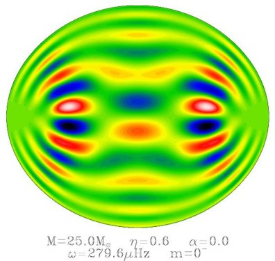
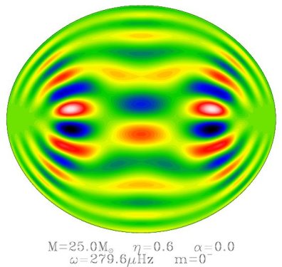
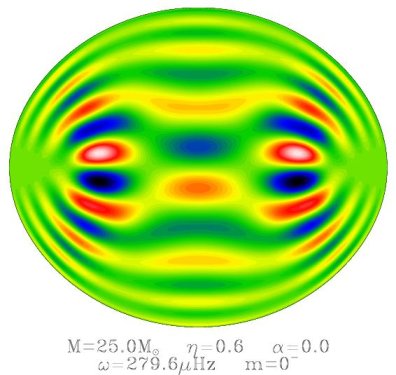
Finite differences	Chebyshev polynomials	Polynomial splines

Figure 2: Comparison of a pulsation mode calculated using finite differences (left), a spectral method (centre), and polynomial splines (right) to discretise the equations in the radial direction. These and other similar plots show a meridional cross-section of the Eulerian pressure perturbation divided by the square root of the background density profile so as to bring out near surface regions. The difference on the frequencies is less than $0.1\,\,\mu$Hz.

Finally, a last test consists in applying different numerical techniques to calculate the eigenmodes and seeing if they give similar results. Figure 2 shows such a comparison. The mode on the left is calculated using $4^{\mathrm{th}}$ order finite differences in the radial direction, the one in the middle a spectral method based on Chebyshev polynomials and the one on the right $4^{\mathrm{th}}$ order polynomial splines. The angular resolution was very similar for the three cases and the radial resolution went from $N_{\mathrm{r}}=101$ for the calculation based on Chebyshev polynomials to $N_{\mathrm{r}}=301$ for the spline-based calculation. As can be seen in the figure, the three calculations yield very similar results, and the corresponding frequencies are less than $0.1\,\,\mu$Hz apart. Furthermore, as will be explained later on, some pulsation modes were calculated using the Lagrangian displacement rather than the Eulerian velocity perturbation. When comparing the two methods, differences on the frequencies are very small for $m=0$ and can be larger for $m\neq 0$ (for example, $\delta\omega/\omega=10^{-3}$ for the mode represented in Fig. 11, right panel), thereby providing yet another verification on the pulsation mode calculations.

Overall, these tests indicate a good numerical stability both with respect to the numerical resolution and the choice of numerical method. The tests on the variational principle, on the other hand, show that some numerical difficulties remain, possibly resulting from a loss of precision on the stellar models. Furthermore, the accuracy is not as good when the rotation rate approaches break-up, as shown in Reese et al. (2008b). Before doing accurate comparisons with actual observations, these difficulties will need to be addressed. Nonetheless, these are not expected to change the basic behaviour of the pulsation modes nor the results in following sections.

3 Uniform or nearly uniform rotation profile

3.1 Mode classification

As was stated above, Lignières & Georgeot (2008) and Lignieres & Georgeot (2009) have previously shown that for rotating polytropic models, pulsation modes fall into the following main categories: island, chaotic, and whispering gallery modes. We have found that a similar classification also applies to pulsation modes in SCF models with uniform or mildly differential rotation (at least up to $\alpha=0.4$, which, based on Eq. (1), gives an equatorial rotation rate which is $84\%$ of the polar rotation rate). Figure 3 compares pulsation modes from both types of models. As can be seen in the figure, corresponding modes with an analogous geometric structure are also present in SCF models.

	Island	Chaotic	Whispering gallery
	Low $\ell-|m|$	Medium $\ell-|m|$	High $\ell-|m|$
Polytropic
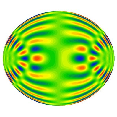
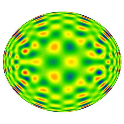
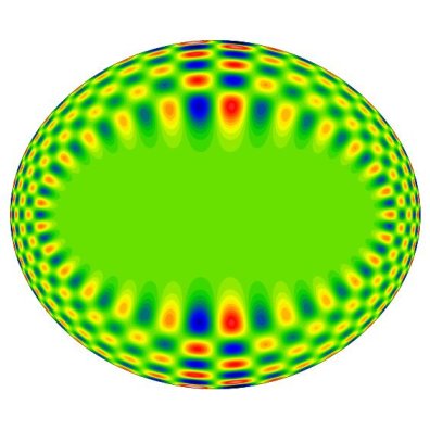
SCF

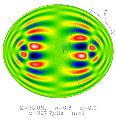
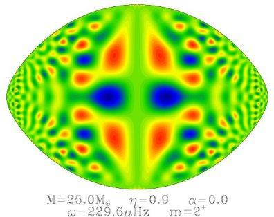
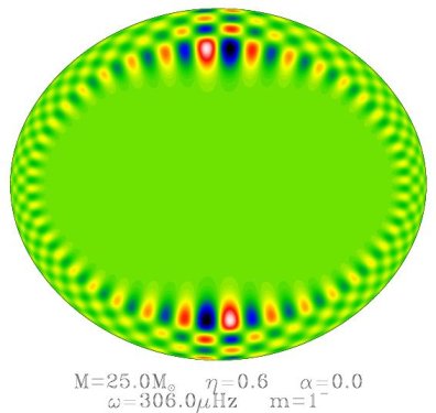
Figure 3: A comparison between pulsation modes in polytropic models and models based on the SCF method. The same three categories apply in both cases as can be seen by the analogous geometric structure. The quantum numbers $\tilde{n}$ and $\tilde{\ell}$, which only apply to island modes, are the number of nodes in the directions indicated in the lower left plot.

3.2 Quantum numbers for island modes

As was also the case for polytropic models, it is possible to introduce a new set of quantum numbers $(\tilde{n},\,\tilde{\ell},m)$ based on the geometry of island modes (see lower left plot in Fig. 3). These quantum numbers then intervene in a new asymptotic formula which describes the frequency organisation of these modes:

$$\omega=\tilde{n}\Delta_{\tilde{n}}+\tilde{\ell}\Delta_{\tilde{\ell}}+m^{2}\Delta_{\tilde{m}}-m\Omega_{\mathrm{fit}}+\tilde{\alpha}$$ (27)

where $\Delta_{\tilde{n}},\,\Delta_{\tilde{\ell}},\,\Delta_{\tilde{m}}$ and $\tilde{\alpha}$ are free parameters which depend on stellar structure. The parameter $\Omega_{\mathrm{fit}}$ corresponds to the rotation rate but is treated as a free parameter. This formula is quite similar to the one introduced in (Lignières & Georgeot 2008, Reese et al. 2008a) except that $|m|$ has been replace by $m^{2}$ as this provides a slightly more accurate fit to the frequencies. The reason why $|m|$ had been obtained in Reese et al. (2008a) is because the formula was first derived for the quantum numbers $(n,\,\ell,\,m)$, where a term proportional to $|m|$ dominates, and then adapted to $(\tilde{n},\,\tilde{\ell},\,m)$.

Table 1 gives the values of these parameters for selected SCF models as well as for a polytropic model. The parameters were calculated from a sparse frequency set and are therefore subject to some error. The ranges on the quantum numbers are $10\leq\tilde{n}\leq 26$, $0\leq\tilde{\ell}\leq 3$ and $-2\leq m\leq 2$. Furthermore, due to difficulties in mode identification, the parameters given for the most rapidly rotating models $(\eta=0.9)$ must be taken with caution. Nonetheless, a second calculation based on a more complete mode set shows that these values provide a reasonable estimate for 2 of the models (see following section). The true value or range of values for the rotation rate, $\Omega_{\mathrm{real}}$, is also provided and shows a posteriori that $\Omega_{\mathrm{fit}}$ does approximately correspond to the rotation rate.

Table 1: Parameters for the asymptotic formula Eq. (27).

$\displaystyle\frac{M}{M_{\odot}}$	$\eta$	$\alpha$	$N_{\mathrm{modes}}$	$\!\!\!\begin{array}[]{c}\displaystyle\Delta_{\tilde{n}}\\ (\mu\mathrm{Hz})\end{array}\!\!\!$	$\displaystyle\frac{\Delta_{\tilde{\ell}}}{\Delta_{\tilde{n}}}$	$\displaystyle\frac{\Delta_{\tilde{m}}}{\Delta_{\tilde{n}}}$	$\displaystyle\frac{\tilde{\alpha}}{\Delta_{\tilde{n}}}$	$\displaystyle\frac{\Omega_{\mathrm{fit}}}{\Delta_{\tilde{n}}}$	$\displaystyle\frac{\Omega_{\mathrm{real}}}{\Delta_{\tilde{n}}}$	$\displaystyle\frac{\left<\delta\omega^{2}\right>^{1/2}}{\Delta_{\tilde{n}}}$
poly⋆	0.6	0.0	84	36.7	0.66	0.029	2.92	0.827	0.838	0.047
1.7	0.7	0.0	40	37.1	0.77	0.018	3.52	0.975	0.982	0.023
1.8	0.9	0.0	11	33.5	0.42	0.011	2.86	1.157	1.167	0.038
25.0	0.6	0.0	39	15.2	0.79	0.016	3.39	0.947	0.969	0.030
25.0	0.6	0.2	31	15.1	0.85	0.018	3.63	0.944	0.947-0.987	0.045
25.0	0.6	0.4	31	15.5	0.90	0.050	3.37	0.915	0.830-0.988	0.059
25.0	0.9	0.0	24	12.4	0.70	-0.002	3.41	1.380	1.387	0.033

• Values of the different parameters from Eq. (27) for selected SCF models as well as for a polytropic model (first line). The first three columns identify the model, where $\eta$ and $\alpha$ come from Eq. (1). These parameters were based on a sparse mode set (the number of modes being indicated by $N_{\mathrm{mode}}$) and are therefore subject to error. The last column contains the average deviation between asymptotic frequencies based on Eq. (27) and the numerical frequencies.

• ^⋆Polytropic model with $N=3$, $M=1.7M_{\odot}$ and $R_{\mathrm{eq}}=1.84R_{\odot}$. These are also the mass and equatorial radius of the model on the next line.

As was noted in Reese et al. (2008a), the ratio $\Delta_{\tilde{\ell}}/\Delta_{\tilde{n}}$ decreases for increasing rotation rates. Using $\Delta_{\ell}/\Delta_{n}=1/2$ in the non-rotating case (Tassoul 1980), and the relationships between $\Delta_{\tilde{n}}$, $\Delta_{\tilde{\ell}}$ and $\Delta_{n}$, $\Delta_{\ell}$ given in Reese et al. (2008a), one finds a theoretical value of $2$ for $\Delta_{\tilde{\ell}}/\Delta_{\tilde{n}}$ when $\Omega=0$. Since the values in Table 1 are much smaller, the “small” frequency separation is no longer small but comparable with the large frequency separation, as was also observed in Lignières et al. (2006) and Lovekin et al. (2009).

In the last column, the standard deviation between the asymptotic and numerical frequencies is given. It is defined as follows:

$$\left<\delta\omega^{2}\right>^{1/2}=\sqrt{\frac{1}{N_{\mathrm{modes}}}\sum_{i=1}^{N_{\mathrm{modes}}}\left(\omega_{i}-\omega_{i}^{\mathrm{asymp.}}\right)^{2}}$$ (28)

where $\omega_{i}^{\mathrm{asymp.}}$ are the frequencies given by the asymptotic formula and $\omega_{i}$ the numerical frequencies. Although the asymptotic formula captures the basic structure of the frequency spectrum (at least for low values of $m$), there are differences which are larger than observational error bars. The main causes seem to be deviations resulting from avoided crossings and also a slight variation of the azimuthal dependence of the frequencies with $\tilde{\ell}$ and $\tilde{n}$ (see following section).

3.3 High azimuthal orders

The results presented so far were based on pulsation modes with azimuthal orders between -2 and 2. However, island modes also exist for high values of $m$ as is illustrated in Fig. 4. As can be seen in the figure, high $m$ island modes have an analogous structure to their low $m$ counterparts except that they are much closer to the equator. This is similar to the behaviour of sectoral modes in non-rotating stars.

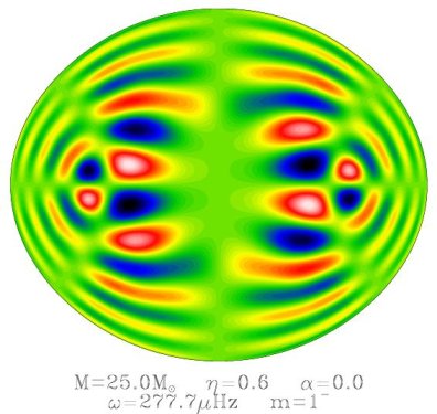
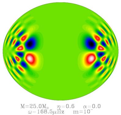
Figure 4: Two island pulsation modes, one with a low $m$ value (left) and the other with a high $m$ value (right). Although the basic structure remains the same, the mode with a high azimuthal order is concentrated much closer to the equator. This is analogous to what happens with sectoral modes in non-rotating stars when $m$ increases.

Figure 5 shows two pulsation frequency spectra with $\tilde{n}=15$ to $20$, $\tilde{\ell}=0$ to $1$ and $m=-10$ to $10$. The left plot is for a uniformly rotating model and the right one corresponds to differential rotation. The symbols represent the numerical frequencies and the continuous lines are a least-squares fit based on the following formula:

$$\omega_{\tilde{n},\,\tilde{\ell},\,m}=\tilde{n}\Delta_{\tilde{n}}+D_{\tilde{m}}(\tilde{\ell})\sqrt{m^{2}+\mu(\tilde{\ell})^{2}}-m\Omega_{\mathrm{fit}}+\tilde{\alpha}(\tilde{\ell}).$$ (29)

The term $m\Omega_{\mathrm{fit}}$ has been removed from both the numerical frequencies and the fit in Fig. 5 so as to bring out their more subtle azimuthal dependence. In Eq. (29), the term with $\Delta_{\tilde{m}}$ has been replaced so as to give the frequencies a hyperbolic dependence on $m$, as is visually suggested by the numerical frequencies. Besides the modification to the azimuthal term, the term $\Delta_{\tilde{\ell}}$ has been removed but is compensated for by allowing the parameters $D_{\tilde{m}}$, $\mu$ and $\tilde{\alpha}$ to depend on $\ell$.

Figure 5: Pulsation frequency spectrum in a uniformly (left panel) and differentially (right panel) rotating model. The radial order $\tilde{n}$ goes from $15$ (bottom) to 20 (top), and $\tilde{\ell}=0$ and $1$. Each hyperbola corresponds to a distinct pair $(\tilde{n},\tilde{\ell})$. The symbols represent the numerically calculated frequencies and the continuous lines correspond to a least-squares fit based on Eq. (27). Some of the irregular features in the numerical frequencies are caused by avoided crossings.

Table 2 gives the values of the different parameters used to fit the frequency spectra in Fig. 5. Comparing these values with those in Table 1 shows reasonable agreement, provided one compares $\Delta_{\tilde{m}}$ and $\Delta_{\tilde{\ell}}$ with $D_{m}/2\mu$ and $\alpha(\tilde{\ell}=1)-\alpha(\tilde{\ell}=0)$, respectively, where the expressions $D_{m}/2\mu$ comes from a Taylor expansion of Eq. (29) around $m=0$. Although the average deviations are larger in this table, Eq. 29 is a better fit to the frequencies than Eq. 27. The reason for this apparent contradiction is because the frequency sets used in Table 2 cover a larger range of $m$ values. Applying Eq. 27 to these expanded sets would yield $\left<\delta\omega^{2}\right>^{1/2}/\Delta_{\tilde{n}}=0.079$ and $0.088$ for the uniformly and differentially rotating models, respectively.

An important difference between the two formulae, is that contrary to what is suggested by Eq. (27), the azimuthal dependence is different for $\tilde{\ell}=0$ and $\tilde{\ell}=1$ modes. A likely cause is the fact that pulsation modes are closer to the equator at high $m$ values. This would then modify the path which intervenes in the time integrals used to calculate $\Delta_{\tilde{\ell}}$, when working with ray dynamics (Lignières & Georgeot 2008). As a result, a physically more relevant formula for the frequencies would include a $\Delta_{\tilde{\ell}}$ term which depends on $m$ rather than an azimuthal term which depends on $\tilde{\ell}$. Of course, a quantitative calculation based on ray dynamics is needed to support this explanation.

Table 2: Parameters for the asymptotic formula Eq. (29).

Stellar parameters						$\tilde{\ell}=0$				$\tilde{\ell}=1$
$\displaystyle\frac{M}{M_{\odot}}$	$\eta$	$\alpha$	$\!\!\!\begin{array}[]{c}\displaystyle\Delta_{\tilde{n}}\\ (\mu\mathrm{Hz})\end{array}\!\!\!$	$\displaystyle\frac{\Omega_{\mathrm{fit}}}{\Delta_{\tilde{n}}}$	$\displaystyle\frac{\Omega_{\mathrm{real}}}{\Delta_{\tilde{n}}}$	$\displaystyle\frac{D_{\tilde{m}}}{\Delta_{\tilde{n}}}$	$\displaystyle\mu$	$\displaystyle\frac{\tilde{\alpha}}{\Delta_{\tilde{n}}}$	$\displaystyle\frac{D_{\tilde{m}}}{2\mu\Delta_{\tilde{n}}}$	$\displaystyle\frac{D_{\tilde{m}}}{\Delta_{\tilde{n}}}$	$\displaystyle\mu$	$\displaystyle\frac{\tilde{\alpha}}{\Delta_{\tilde{n}}}$	$\displaystyle\frac{D_{\tilde{m}}}{2\mu\Delta_{\tilde{n}}}$	$\displaystyle\frac{\left<\delta\omega^{2}\right>^{1/2}}{\Delta_{\tilde{n}}}$
25	0.6	0.0	14.91	0.980	0.989	0.197	5.95	2.67	0.0166	0.234	5.11	3.41	0.0229	0.045
25	0.6	0.2	15.01	0.962	0.953-0.993	0.221	6.04	2.50	0.0183	0.244	4.52	3.52	0.0270	0.052

• Values of the parameters from Eq. (29) used to fit the frequencies in Fig. 5 (i.e. the ranges on the quantum numbers are $15\leq\tilde{n}\leq 20$, $0\leq\tilde{\ell}\leq 1$ and $-10\leq m\leq 10$). These values are similar to those in Table 1 (see text for details). The two values of $\Omega_{\mathrm{real}}$ for the differentially rotating model (second line) are the lower and upper on the angular velocity, i.e. the equatorial and polar rotation rates, respectively. The parameter $\Omega_{\mathrm{fit}}$ is twice as close to $\Omega_{\mathrm{real}}$ as in Table 1 for the uniformly rotating model ($\alpha=0$) due to the inclusion of higher azimuthal orders.

It is also interesting to look at what happens when $\tilde{n}$ is increased to a large value. Figure 6 compares 4 sets of pulsation frequencies corresponding to $\tilde{n}=20$, $40$, $50$ and $60$. The symbols represent the numerical frequencies and the continuous lines a fit based on Eq. (29). The frequencies are given in a co-rotating frame and have been shifted so that the different curves are at $0$ for $m/\sqrt{n}=0$. Plotting the frequencies as a function of $m/\sqrt{\tilde{n}}$ rather than $m$ causes the curves associated with the high order frequencies to overlap and reduces the difference between these curves and the $\tilde{n}=20$ curve. These results suggest that as $\tilde{n}$ goes to infinity, the azimuthal dependence of the co-rotating frequencies can be described by a law of the form $n^{\delta}f\left(m/n^{\gamma}\right)$ where $f$ is a function and $2\gamma-\delta=1$.

Figure 6: Four sets of pulsation frequencies in a co-rotating frame in which $\tilde{n}=20$, $40$, $50$ and $60$. The other quantum numbers are $\tilde{\ell}=0$ and $m=-10$ to $10$ for all sets. The azimuthal order has been scaled by $1/\sqrt{\tilde{n}}$ as this causes the high order curves to overlap and reduces the difference between these curves and the $\tilde{n}=20$ curve.

3.4 An effective rotation rate

Of particular interest is the parameter $\Omega_{\mathrm{fit}}$. In the uniformly rotating case, the term $-m\Omega_{\mathrm{fit}}$ represents, to first order, the advection of the modes by stellar rotation. The value given for $\Omega_{\mathrm{fit}}$ in Table 2 is quite close to the true rotation rate and only differs by $0.93\%$, this difference probably resulting from the Coriolis force. In the differentially rotating case, $-m\Omega_{\mathrm{fit}}$ can also be interpreted as an estimate of the advection of the pulsation modes by stellar rotation. The parameter $\Omega_{\mathrm{fit}}$ would then be an average of the rotation rate in which the weighting depends on the structure of the pulsation modes. We will refer to $\Omega_{\mathrm{fit}}$ as an effective rotation rate. We can then use Eq. (1) to calculate the position $s_{\mathrm{fit}}$ where $\Omega(s)$ is equal to $\Omega_{\mathrm{fit}}$ for the differentially rotating model. This is represented by the thick vertical line in Fig. 7 for the numerical value given in Table 2. The hashed region on either side of this line is an estimate of the error on this position using the difference between $\Omega_{\mathrm{fit}}$ and $\Omega_{\mathrm{real}}$ from the uniformly rotating model as a guide.

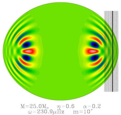
Figure 7: The $(\tilde{n},\,\tilde{\ell},\,m)=(20,0,10)$ island mode in the differentially rotating model. The vertical thick line corresponds to the position where $\Omega_{\mathrm{fit}}$ is equal to the local rotation rate. The hashed region on either side is an estimate of the error on this position, based on the difference between $\Omega_{\mathrm{fit}}$ and $\Omega_{\mathrm{real}}$ for the uniformly rotating model.

As can be seen from Fig. 7, $s_{\mathrm{fit}}$ is located towards the outer regions of the star. This means that $\Omega_{\mathrm{fit}}$, when viewed as an average of the rotation profile, has a stronger weighting in these outer regions. This seems logical from the point of view of ray dynamics because a sound wave travelling along a ray path will spend most of its time in the outer regions of the star where the local sound velocity is lower. As a result, it will spend more time being advected by rotation in that region rather than in an inner region. Sound-travel times along ray paths have already been used to establish an asymptotic expression for rotational kernels of high order p-modes in spherical stars (Gough 1984).

One of the best ways to confirm these ideas in a quantitative way is to apply a variational formula which is valid for differential rotation. Such a formula has been established in Lynden-Bell & Ostriker (1967). Here we give a different and somewhat simpler expression which is only valid for conservative rotation profiles:

$$0 = \int_{V}(\omega_{\mathrm{var}}+m\Omega)^{2}\rho_{o}\|\@vec{\xi}\|^{2}dV+2i\int_{V}(\omega_{\mathrm{var}}+m\Omega)\rho_{o}\@vec{\Omega}\cdot\left(\@vec{\xi}^{*}\times\@vec{\xi}\right)dV$$ (30)

$$-\int_{V}\rho_{o}\left|\xi_{s}\right|^{2}s\partial_{s}\left(\Omega^{2}\right)dV-\int_{V}\frac{|p|^{2}dV}{\rho_{o}c_{o}^{2}}-\int_{V}\rho_{o}N_{o}^{2}\left|\xi_{g}\right|^{2}dV+\frac{1}{\Lambda}\int_{V_{\infty}}\|\@vec{\nabla}\Psi\|^{2}dV,$$

where $\@vec{\xi}$ is the Lagrangian displacement, $\xi_{s}$ the displacement component perpendicular to the rotation axis and $\xi_{g}$ the displacement component in the same direction as the effective gravity. In order to apply this formula, it is necessary to calculate pulsation modes in terms of $\@vec{\xi}$ rather than $\@vec{v}$, the Eulerian velocity perturbation. This has been done, and the relevant pulsation equations are described in App. A.

In the uniformly rotating case, the term that corresponds to the advection of pulsation modes by rotation is $m\Omega$, which is contained in the first integral. By analogy, we can define an effective rotation rate for the differentially rotating case as follows:

$$\int_{V}(\omega_{\mathrm{var}}+m\Omega)^{2}\rho_{o}|\@vec{\xi}|^{2}dV=(\omega_{\mathrm{var}}+m\Omega_{\mathrm{eff}})^{2}\int_{V}\rho_{o}|\@vec{\xi}|^{2}dV$$ (31)

Solving for $\Omega_{\mathrm{eff}}$ leads to the following expression:

$$\Omega_{\mathrm{eff}}=-\frac{\omega_{\mathrm{var}}}{m}+\frac{1}{m}\sqrt{\int_{V}\left(\omega_{\mathrm{var}}+m\Omega\right)^{2}\mathcal{K}dV},$$ (32)

where

$$\mathcal{K}=\frac{\rho_{o}\|\xi\|^{2}}{\int_{V}\rho_{o}\|\xi\|^{2}dV}.$$ (33)

When $m\Omega\ll 2\omega$, then $\Omega_{\mathrm{eff}}$ can be approximated by $\int_{V}\Omega\mathcal{K}dV$. This is similar to the first order perturbative expression describing the advection of modes by slow rotation, except that the kernel $\mathcal{K}$ has been defined from the eigenmode in the rotation star. Figure 8 shows a plot of the kernel associated with the mode in Fig. 7. As can be seen in the figure, the highest amplitudes are reached very near the surface, just like for acoustic modes of non-rotating stars. Superimposed on the diagram is a vertical lines which indicates the position of $s_{\mathrm{fit}}^{\mathrm{eff}}=\Omega^{-1}\left(\Omega_{\mathrm{eff}}\right)$. This can be compared with $s_{\mathrm{fit}}$ which is plotted in Fig. 7. As can be seen from the two figures, $s_{\mathrm{fit}}^{\mathrm{eff}}<s_{\mathrm{fit}}$. This difference comes from the fact that $s_{\mathrm{fit}}$ not only includes the advection of modes by rotation but also the effects of the Coriolis force on the mode frequencies.

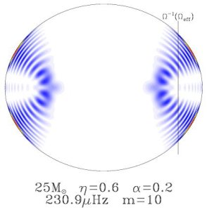
Figure 8: A plot of the kernel associated with the $(\tilde{n},\,\tilde{\ell},\,m)=(20,0,10)$ mode shown in Fig. 7. As can be seen, the highest amplitudes are reached very near the surface, just like for p-modes in non-rotating stars. The vertical line indicates the position of $s_{\mathrm{fit}}^{\mathrm{eff}}=\Omega^{-1}\left(\Omega_{\mathrm{eff}}\right)$ which can be compared with the position of $s_{\mathrm{fit}}$ as shown in Fig. 7.

The rotation rate $\Omega_{\mathrm{eff}}$ turns out to be a very good indicator of the advection of modes by rotation. This is illustrated in Fig. 9, which shows a comparison between $\left(\omega_{\tilde{n},\,\tilde{\ell},\,m}-\omega_{\tilde{n},\,\tilde{\ell},\,-m}\right)/2m$ (solid line) and $\left(\Omega_{\mathrm{eff}}(m)+\Omega_{\mathrm{eff}}(-m)\right)/2$ (dotted line), for a set of modes in which the Coriolis force has been removed. The relative difference between the two is around $10^{-6}-10^{-5}$, making it difficult to distinguish the two curves. The downward trend results from the fact that the pulsation modes are becoming closer to the equator as $|m|$ increases. The dent between $m=5$ and $m=6$ is caused by an avoided crossing. Also, the curves corresponding to $\Omega_{\mathrm{eff}}(m)$ and $\Omega_{\mathrm{eff}}(-m)$ have been included. The reason why these curves are not identical is because modes with azimuthal orders $m$ and $-m$ are not identical even without the Coriolis force, because of the differential rotation profile.

Figure 9: Different measures of the effective rotation rate. The solid and dotted curves show an average over $m$ and $-m$ of $\Omega_{\mathrm{eff}}$ based on the numerical frequencies and on Eq. (32). The two last curves show the separate contributions from $m$ and $-m$, where $m$ corresponds to retrograde modes and $-m$ to prograde modes.

This naturally leads on to the idea of applying inversion theory to probe the rotation profile using the rotational kernels defined in Eq. (33). The quantity $\left(\omega_{\tilde{n},\,\tilde{\ell},\,m}-\omega_{\tilde{n},\,\tilde{\ell},\,-m}\right)/2m$ is readily available from observations, once an accurate mode identification has been done. Furthermore, it turns out that $\Omega^{1}_{\mathrm{eff}}=\int_{V}\Omega\mathcal{K}dV$ is a very good approximation to $\Omega_{\mathrm{eff}}$, at least in the example considered above, thereby allowing the use of linear inversion theory. These kernels will, nonetheless, need to refined so as to include the effects of the Coriolis force.

4 Highly differential rotation

When the rotation profile becomes highly differential, the stellar structure becomes more and more deformed and the polar regions can, in some cases, become concave. These polar concavities result from the particular choice of rotation profile as expressed in Eq. (1) since they do not appear in models where the rotation rate increases with distance from the rotation axis. This deformation naturally affects the structure and organisation of pulsation modes. Figure 10 shows a chaotic and what appears to be a whispering gallery mode in models where the rotation profile is very differential. No island modes are shown as they seem to have disappeared. In the more distorted configurations, even whispering gallery modes become difficult to find. Instead, most of the modes are of a very chaotic nature.

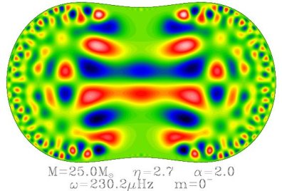
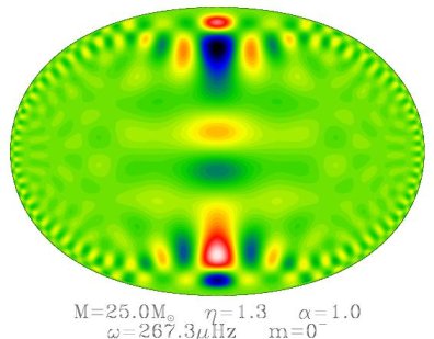
Figure 10: The left figure corresponds to a chaotic mode and the right one to what appears to be a whispering gallery mode in SCF models with a highly differential rotation profile. No island modes are shown as they seem to have disappeared in the models (for low $m$).

One way to counteract the effects of stellar distortion is to increase the azimuthal order $m$. Indeed, increasing the azimuthal order causes the pulsation modes to become closer to the equator and move away from the poles where stellar deformation is strongest. As can be seen in Fig. 11, highly regular whispering gallery modes exist even in the most deformed configurations. Also, for models with less distortion, it is possible to find some island modes. Nonetheless, such modes are not likely to be visible in stars due to disk averaging effects. Therefore, if stars reach this degree of distortion, it will be very challenging to interpret their pulsation spectra.

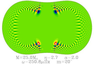
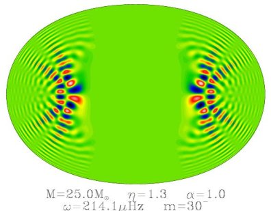
Figure 11: The two figures corresponds to pulsation modes with a high azimuthal orders in models with a highly differential profile. The left figure corresponds to a whispering gallery mode and the right one to an island mode. As can be seen in these plots, pulsation modes become less chaotic with increasing azimuthal order.

5 Conclusion

As has been shown in this paper, results concerning pulsation modes in rapidly rotating polytropic models can be generalised to more realistic models based on the Self-Consistent Field method (Jackson et al. 2005, MacGregor et al. 2007) provided the rotation profile is not too differential. In particular, pulsation modes fall into different categories, island, chaotic and whispering gallery modes, each with their own characteristic geometry, in full agreement with previous calculations based on ray dynamics (Lignières & Georgeot 2008, Lignieres & Georgeot 2009). The frequencies of the island modes obey the same type of asymptotic formula as those in polytropic models although a more careful investigation of their $m$-dependence reveals a more complex behaviour than was previously established. This type of formula potentially provides a promising way of identifying pulsation modes in rapidly rotating stars, especially at high radial orders where the agreement between formula and frequency is very good (Reese et al. 2009). Of course, when applying this formula to observations, one should restrict themselves to modes with low $\tilde{\ell}$ and $m$ values, because cancellation effects reduce the visibility of modes with more nodes on the surface. As a result, the approximate form given by Eq. 27, which is valid for low $m$ values, is sufficiently accurate.

A useful by-product of the asymptotic formula is an estimate of the effective rotation rate which gives the average advection of modes by rotation when the rotation profile is mildly differential. The obtained value indicates a stronger weighting near the surface, where the local sound velocity is smaller. This goes hand in hand with the intuitive picture based on ray dynamics that a sound wave is most advected in those regions where it spends the most time. A rigorous calculation based on a variational principle yields rotation kernels which confirm this picture and help provide effective rotation rates similar to the one obtained in the asymptotic formula, apart from the effects of the Coriolis force on the frequencies. These rotation kernels could then be used in inversion methods to probe the rotation profile.

When the rotation profile is highly differential, pulsation modes tend to be predominantly chaotic, probably as a result of the star’s geometric distortion. Increasing the azimuthal order counteracts this effect by drawing the pulsation modes closer to the equator thereby causing regular whispering gallery modes, and in some cases, island modes, to reappear. Nonetheless, such modes are not likely to be visible due to disk averaging effects thus making pulsation spectra in such stars difficult to interpret.

Appendix A Pulsation equations based on the Lagrangian displacement

In order to derive the Euler’s equation in terms of the Lagrangian displacement, we begin with Eq. 13 of Lynden-Bell & Ostriker (1967) and calculate its Eulerian perturbation in an inertial frame:

$$\rho_{o}\frac{D_{o}^{2}\@vec{\xi}}{Dt^{2}}-\rho_{o}\@vec{\xi}\cdot\@vec{\nabla}\left(\@vec{v}_{o}\cdot\@vec{\nabla}\@vec{v}_{o}\right)=-\@vec{\nabla}p+\rho\@vec{g}_{\mathrm{eff}}-\rho_{o}\@vec{\nabla}\Psi,$$ (34)

where $\xi$ is the Lagrangian displacement, and other quantities have the same definitions as before. The time derivation operator is defined as follows:

$$\frac{D_{o}\@vec{\xi}}{Dt}=\frac{\partial\@vec{\xi}}{\partial t}+\@vec{v}_{o}\cdot\@vec{\nabla}\@vec{\xi}=\lambda\@vec{\xi}+\@vec{\Omega}\times\@vec{\xi}+im\Omega\@vec{\xi}.$$ (35)

Simplifying Eq. 34 yields:

$$\left[\lambda+im\Omega\right]^{2}\rho_{o}\@vec{\xi}+2\left[\lambda+im\Omega\right]\rho_{o}\@vec{\Omega}\times\@vec{\xi}+\rho_{o}\xi_{s}s\partial_{s}\left(\Omega^{2}\right)\@vec{e}_{s}=-\@vec{\nabla}p+\rho\@vec{g}_{\mathrm{eff}}-\rho_{o}\@vec{\nabla}\Psi.$$ (36)

This is the same equation as what is used in Lovekin et al. (2009). If one uses the following relationship between $\@vec{\xi}$ and $\@vec{v}$ (e.g. Christensen-Dalsgaard 2003):

$$\@vec{v}=\frac{\partial\@vec{\xi}}{\partial t}+\@vec{v}_{o}\cdot\@vec{\nabla}\@vec{\xi}-\@vec{\xi}\cdot\@vec{\nabla}\@vec{v}_{o},$$ (37)

it is possible to show that Eq. 6 and Eq. 36 are equivalent.

In terms of the coordinate system described in Section 2.3, Euler’s equation takes on the following explicit form:

$$0 = \left[\omega+m\Omega\right]^{2}\rho_{o}\left[\frac{\zeta^{2}r_{\zeta}\xi^{\zeta}}{r^{2}}+\frac{\zeta r_{\theta}\xi^{\theta}}{r^{2}}\right]+2i\left[\omega+m\Omega\right]\frac{\Omega\zeta\sin\theta}{r}\rho_{o}\xi^{\phi}$$ (38)

$$-\rho_{o}s\left(\partial_{s}\Omega^{2}\right)r_{\zeta}\sin\theta\left[\frac{\zeta^{2}\sin\theta}{r^{2}}\xi^{\zeta}+\frac{\zeta\left(r_{\theta}\sin\theta+r\cos\theta\right)}{r^{2}r_{\zeta}}\xi^{\theta}\right]-\partial_{\zeta}p+\frac{\partial_{\zeta}P_{o}}{\rho_{o}}\rho-\rho_{o}\partial_{\zeta}\Psi,$$

$$0 = \left[\omega+m\Omega\right]^{2}\rho_{o}\left[\frac{\zeta^{2}r_{\theta}\xi^{\zeta}}{r^{2}}+\frac{\zeta(r^{2}+r_{\theta}^{2})\xi^{\theta}}{r^{2}r_{\zeta}}\right]+2i\left[\omega+m\Omega\right]\frac{\Omega\zeta\left(r_{\theta}\sin\theta+r\cos\theta\right)}{rr_{\zeta}}\rho_{o}\xi^{\phi}$$ (39)

$$-\rho_{o}s\left(\partial_{s}\Omega^{2}\right)\left(r_{\theta}\sin\theta+r\cos\theta\right)\left[\frac{\zeta^{2}\sin\theta}{r^{2}}\xi^{\zeta}+\frac{\zeta\left(r_{\theta}\sin\theta+r\cos\theta\right)}{r^{2}r_{\zeta}}\xi^{\theta}\right]-\partial_{\theta}p+\frac{\partial_{\theta}P_{o}}{\rho_{o}}\rho-\rho_{o}\partial_{\theta}\Psi,$$

$$0 = \left[\omega+m\Omega\right]^{2}\rho_{o}\frac{\zeta}{r_{\zeta}}\xi^{\phi}-2i\left[\omega+m\Omega\right]\frac{\Omega\zeta^{2}\sin\theta}{r}\rho_{o}\xi^{\zeta}-2i\left[\omega+m\Omega\right]\frac{\Omega\zeta\left(r_{\theta}\sin\theta+r\cos\theta\right)}{rr_{\zeta}}\rho_{o}\xi^{\theta}-\frac{\partial_{\phi}p}{\sin\theta}-\rho_{o}\frac{\partial_{\phi}\Psi}{\sin\theta}.$$ (40)

where $i\omega=\lambda$. This is then supplemented by the the continuity equation,

$$0=\rho+\@vec{\nabla}\cdot\left(\rho_{o}\@vec{\xi}\right),$$ (41)

the adiabatic relation,

$$0=p+\@vec{\xi}\cdot\@vec{\nabla}p_{o}-c_{o}^{2}\left(\rho+\@vec{\xi}\cdot\@vec{\nabla}\rho_{o}\right),$$ (42)

and Poisson’s equation,

$$0=\Delta\Psi-\Lambda\rho,$$ (43)

which in spheroidal geometry are:

$$0 = \rho+\frac{\zeta^{2}\partial_{\zeta}\rho_{o}\xi^{\zeta}+\zeta\partial_{\theta}\rho_{o}\xi^{\theta}}{r^{2}r_{\zeta}}+\frac{\zeta^{2}\rho_{o}}{r^{2}r_{\zeta}}\left[\frac{\partial_{\zeta}\left(\zeta^{2}\xi^{\zeta}\right)}{\zeta^{2}}+\frac{\partial_{\theta}\left(\sin\theta\xi^{\theta}\right)}{\zeta\sin\theta}+\frac{\partial_{\phi}\xi^{\phi}}{\zeta\sin\theta}\right],$$ (44)

$$0 = \left(p-c_{o}^{2}\rho\right)+\frac{\zeta^{2}}{r^{2}r_{\zeta}}\left(\partial_{\zeta}p_{o}-c_{o}^{2}\partial_{\zeta}\rho_{o}\right)\xi^{\zeta}+\frac{\zeta}{r^{2}r_{\zeta}}\left(\partial_{\theta}p_{o}-c_{o}^{2}\partial_{\theta}\rho_{o}\right)\xi^{\theta},$$ (45)

$$0 = \frac{r^{2}+r_{\theta}^{2}}{r^{2}r_{\zeta}^{2}}\partial^{2}_{\zeta\zeta}\Psi+c_{\zeta}\partial_{\zeta}\Psi-\frac{2r_{\theta}}{r^{2}r_{\zeta}}\partial^{2}_{\zeta\theta}\Psi+\frac{1}{r^{2}}\Delta_{\theta\phi}\Psi-\Lambda\rho.$$ (46)

Using this set of equation yields the same modes and similar frequencies as using the system of equations based on the Eulerian velocity perturbation $\@vec{v}$. This approach nonetheless has the advantage of yielding $\@vec{\xi}$ which can be used more readily in the variational formula for differential rotation.

References

- Alexander & Ferguson (1994) Alexander, D. R. & Ferguson, J. W. 1994, ApJ, 437, 879
- Bonazzola et al. (1998) Bonazzola, S., Gourgoulhon, E., & Marck, J.-A. 1998, Phys. Rev. D, 58, 104020
- Breger & Pamyatnykh (2006) Breger, M. & Pamyatnykh, A. A. 2006, Memorie della Societa Astronomica Italiana, 77, 295
- Caughlin & Fowler (1988) Caughlin, G. R. & Fowler, W. A. 1988, Atomic Data and Nuclear Data Tables, 40, 283
- Chatelin (1988) Chatelin, F. 1988, Valeurs propres de matrices (Paris : Masson)
- Christensen-Dalsgaard (2003) Christensen-Dalsgaard, J. 2003, Lecture Notes on Stellar Oscillations, http://astro.phys.au.dk/jcd/oscilnotes/
- Christensen-Dalsgaard & Mullan (1994) Christensen-Dalsgaard, J. & Mullan, D. J. 1994, MNRAS, 270, 921
- Clement (1978) Clement, M. J. 1978, ApJ, 222, 967
- Cowling & Newing (1949) Cowling, T. G. & Newing, R. A. 1949, ApJ, 109, 149
- Deupree (1990) Deupree, R. G. 1990, ApJ, 357, 175
- Deupree (1995) Deupree, R. G. 1995, ApJ, 439, 357
- Dintrans & Rieutord (2000) Dintrans, B. & Rieutord, M. 2000, A&A, 354, 86
- Dziembowski & Goode (1992) Dziembowski, W. A. & Goode, P. R. 1992, ApJ, 394, 670
- Eggleton et al. (1973) Eggleton, P. P., Faulkner, J., & Flannery, B. P. 1973, A&A, 23, 325
- Espinosa et al. (2004) Espinosa, F., Pérez Hernández, F., & Roca Cortés, T. 2004, in ESA SP-559: SOHO 14 Helio- and Asteroseismology: Towards a Golden Future, 424–427
- Gough (1984) Gough, D. O. 1984, Royal Society of London Philosophical Transactions Series A, 313, 27
- Gough & Thompson (1990) Gough, D. O. & Thompson, M. J. 1990, MNRAS, 242, 25
- Graboske et al. (1973) Graboske, H. C., Dewitt, H. E., Grossman, A. S., & Cooper, M. S. 1973, ApJ, 181, 457
- Jackson (1970) Jackson, S. 1970, ApJ, 161, 579
- Jackson et al. (2004) Jackson, S., MacGregor, K. B., & Skumanich, A. 2004, ApJ, 606, 1196
- Jackson et al. (2005) Jackson, S., MacGregor, K. B., & Skumanich, A. 2005, ApJS, 156, 245
- Karami et al. (2005) Karami, K., Christensen-Dalsgaard, J., Pijpers, F. P., Goupil, M.-J., & Dziembowski, W. A. 2005, arXiv, astro-ph/0502194
- Kippenhahn et al. (1967) Kippenhahn, R., Weigert, A., & Hofmeister, E. 1967, Meth. Comp. Phys., 7, 129
- Ledoux (1951) Ledoux, P. 1951, ApJ, 114, 373
- Lignières & Georgeot (2008) Lignières, F. & Georgeot, B. 2008, Phys. Rev. E, 78, 016215
- Lignieres & Georgeot (2009) Lignieres, F. & Georgeot, B. 2009, A&A, in press, astro-ph/0903.1768
- Lignières et al. (2006) Lignières, F., Rieutord, M., & Reese, D. 2006, A&A, 455, 607
- Lignières et al. (2001) Lignières, F., Rieutord, M., & Valdettaro, L. 2001, in SF2A-2001: Semaine de l’Astrophysique Francaise, ed. F. Combes, D. Barret, & F. Thévenin, 127
- Lovekin & Deupree (2008) Lovekin, C. C. & Deupree, R. G. 2008, ApJ, 679, 1499
- Lovekin et al. (2009) Lovekin, C. C., Deupree, R. G., & Clement, M. J. 2009, ApJ, 693, 677
- Lynden-Bell & Ostriker (1967) Lynden-Bell, D. & Ostriker, J. P. 1967, MNRAS, 136, 293
- MacGregor et al. (2007) MacGregor, K. B., Jackson, S., Skumanich, A., & Metcalfe, T. S. 2007, ApJ, 663, 560
- Ostriker & Mark (1968) Ostriker, J. P. & Mark, J. W.-K. 1968, ApJ, 151, 1075
- Ouazzani et al. (2009) Ouazzani, R.-M., Goupil, M.-J., Dupret, M.-A., & Reese, D. 2009, in 38th Liège International Astrophysical Colloquium, submitted
- Reese (2006) Reese, D. 2006, PhD thesis, Université Toulouse III - Paul Sabatier, http://tel.archives-ouvertes.fr/tel-00120334
- Reese et al. (2006) Reese, D., Lignières, F., & Rieutord, M. 2006, A&A, 455, 621
- Reese et al. (2008a) Reese, D., Lignières, F., & Rieutord, M. 2008a, A&A, 481, 449
- Reese et al. (2008b) Reese, D., MacGregor, K. B., Jackson, S., Skumanich, A., & Metcalfe, T. S. 2008b, in SF2A-2008, ed. C. Charbonnel, F. Combes, & R. Samadi, 531
- Reese et al. (2009) Reese, D. R., Thompson, M. J., MacGregor, K. B., et al. 2009, submitted to A&A
- Rieutord (2006a) Rieutord, M. 2006a, EAS Publications Series, 21, 275
- Rieutord (2006b) Rieutord, M. 2006b, A&A, 451, 1025
- Rogers & Iglesias (1992) Rogers, F. J. & Iglesias, C. A. 1992, ApJS, 79, 507
- Saio (1981) Saio, H. 1981, ApJ, 244, 299
- Schou et al. (1998) Schou, J., Antia, H. M., Basu, S., et al. 1998, ApJ, 505, 390
- Soufi et al. (1998) Soufi, F., Goupil, M.-J., & Dziembowski, W. A. 1998, A&A, 334, 911
- Tassoul (1980) Tassoul, M. 1980, ApJS, 43, 469
- Thompson et al. (2003) Thompson, M. J., Christensen-Dalsgaard, J., Miesch, M. S., & Toomre, J. 2003, 41, 599
- Vandenberg (1983) Vandenberg, D. A. 1983, ApJS, 51, 29
- Zahn (1974) Zahn, J.-P. 1974, in IAU Symposium, Vol. 59, Stellar Instability and Evolution, ed. P. Ledoux, A. Noels, & A. W. Rodgers, 185–194
- Zahn (1993) Zahn, J.-P. 1993, in Les Houches Summer School Proceedings (1987), ed. J.-P. Zahn & J. Zinn-Justin, 565–615