Practical implementation and error bound
of integer-type algorithm
for higher-order differential equations

Abstract

In our preceding paper, we have proposed an algorithm for obtaining finite-norm solutions of higher-order linear ordinary differential equations of the Fuchsian type $\displaystyle\Bigl{(}\sum_{m=0}^{M}p_{m}(x)\bigl{(}\frac{d}{dx}\bigr{)}^{m}\Bigr{)}f(x)=0$ (where $p_{m}$ is a rational function with rational-number-valued coefficients), by using only the four arithmetical operations on integers, and we proved its validity. For any nonnegative integer $\displaystyle\,k$, it is guaranteed mathematically that this method can produce all the solutions satisfying $\,\int|f(x)|^{2}\,(x^{2}+1)^{k}\,dx<\infty\,$, under some conditions. We materialize this algorithm in practical procedures. An integer-type quasi-orthogonalization used there can suppress the explosion of calculations. Moreover, we give an upper limit of the errors. We also give some results of numerical experiments and compare them with the corresponding exact analytical solutions, which show that the proposed algorithm is successful in yielding solutions with an extraordinarily high accuracy (using only arithmetical operations on integers).

Keywords

key words: higher-order linear ODE, rational-type smooth basis function, numerical analysis, integer-type algorithm, quasi-orthogonalization, error bound.

AMS: 65L99, 42C15, 65L70, 65L60, 34A45

1 Introduction

Since linear higher-order ordinary equations with general coefficient functions cannot be solved analytically except in very special simple cases  [1], numerical methods are useful in many applications, such as the eigenfunction problem for a differential operator on a complete function space ${\cal H}$. Many approaches with numerical methods have been proposed for this problem. One method is based on the approximation of solutions in a finite-dimensional subspace of the original function space ${\cal H}$  [2] [3].

Using an idea somewhat similar to this approach, our preceding paper [4] proved the validity of our newly-proposed integer-type numerical method using smooth (i.e. analytical) basis functions which was able to obtain approximations of all the true solutions in ${\cal H}$ of the Fuchsian-type differential equation $\displaystyle\Bigl{(}\sum_{m=0}^{M}r_{m}(x)\bigl{(}\frac{d}{dx}\bigr{)}^{m}\Bigr{)}f(x)=0$ with rational-function-type coefficient functions $r_{m}(x)$ using only the four arithmetical operations on integers, for a class of complete function spaces ${\cal H}$ containing $L^{2}(\mathbb{R})$ as a special case. This algorithm can be applied even for the non-Fuchsian cases, under some restrictions. However, the method proposed in that paper is considerably different from the usual methods based on approximation in a finite-dimensional subspace, such as the Ritz and Galerkin methods [2] [3]. The main differences from usual Galerkin methods were explained in the introduction of [4]. The method proposed in [4] can be regarded as a kind of ‘semi-analytical method’ rather than a purely numerical method, in that it is closely related to the functional analysis, Fourier series and the Laurent expansion of complex functions. In addition, as a remarkable characteristic of the proposed method, all the basis functions used there are rational functions of the coordinate which are related to a power series of the Cayley transform of the coordinate. This characteristic enables us to close all procedures in the method only within four arithmetic operations between rational numbers and hence between integers. These facts imply that the proposed method can be discussed from some viewpoints of mathematical analysis.

This method is perfectly free from round-off error because it consists only of integer-type operations, when we choose function spaces and their basis systems appropriately. It has only two types of errors instead of round-off errors. One is the ‘pure’ truncation error due to the components outside the subspace (contained even in true exact solutions), and the other is the ‘mixture error’ due to the (slight) mixture of extra solutions not corresponding to true solutions in ${\cal H}$. However, as is proved in  [4], the latter mixture error converges to zero as the dimension of the subspace tends to infinity, with this method. Moreover, the ‘pure’ truncation error decays very rapidly in the proposed method, due to the relationship between the Fourier series and the expansion used in the proposed method.

Moreover, this method requires a small amount of calculations for obtaining high-accuracy solutions. For example, when the coefficients in the expansion of a true solution by the basis functions decay exponentially, the amount of calculations required by this method is almost proportional asymptotically to the cube of the number of required significant digits. This is a strong advantage in comparison with the Runge-Kutta methods and the finite elements methods which require the amount of calculations with exponential orders of the required significant digits. From this advantage, as is shown later in numerical results, by the proposed method, we can easily attain the accuracy with several hundred or several thousand significant digits by an ordinary personal computer in many cases.

Since the structure and the procedures of this method are somewhat complicated, in our preceding paper  [4], we explained only its abstract structure, its mathematical validity and a rough sketch of the procedures in the proposed algorithms. In this paper, we will explain the concrete materialization of this method, and will provide some theoretical analysis of the accuracy of this method.

In the previous paper [4], we have not explained how to calculate the matrix elements of the band-diagonal matrix efficiently in a concrete discussion. In this paper, we will show that we can calculate them from a small number of coefficients which can be derived easily from the recursion formulae among the basis functions only by four arithmetic operations among integers when the coefficients in the rational functions $p_{m}(x)$ $(m=0,1,\dots,M)$ are rational complex numbers. Moreover, we will explain the detailed procedure of a quasi-minimization of the ratio between two quadratic forms which is effective in removing extra solutions of the system of simultaneous linear equations, while it has been omitted in [4]. We will propose and illustrate in detail an integer-type quasi-orthogonalization, which is effective in the above quasi-minimization and requires a relatively small amount of calculations.

The proof of the convergence to true solutions of the numerical solutions obtained by means of this quasi-orthogonalization is one of the main result of this paper. Moreover, we will prove the halting of this process. Another main result of this paper is the proof of an inequality which gives an upper bound of errors contained in numerical solutions obtained by the proposed method.

The contents of this paper are as follows: In Section 2, we survey the basic structures of this method proposed and proved in [4]. In section 3, the function spaces and the basis systems used in this method are surveyed. In section 4, we explain how to calculate the ‘matrix elements’ of the matrix representation of a differential operator using only the coefficients of the differential operator. In Section 5, we specify the concrete procedures for the algorithm proposed only abstractly in [4], for the cases where the space of true solutions in ${\cal H}$ is one-dimensional. In Section 6, we prove that the realization proposed in Section 5 satisfies the conditions required for the convergence of the mixture error to zero. In Section 7, we extend the realization proposed in Section 5 to general cases where the space of obtainable true solutions in ${\cal H}$ is multi-dimensional, and we prove the convergence of the mixture error to zero even for this extension in Section 8. Since the procedures proposed in Section 5 contain iterations under given conditions, we prove that they halt in a finite number of steps in Section 9. In Section 10, we will state a theoretical upper bound for the errors. In Section 11, we give numerical results which clarifies how accurate results our method gives. Moreover, in that section, we compare theoretically the order of the amount of required calculations between some typical existing methods and the proposed method. Finally, we present our conclusions.

2 Survey of basic structure

As was introduced in  [4], we propose an integer-type algorithm for finding the $C^{M}$-solutions in a function space ${\cal H}$ of a higher-order linear ordinary differential equation $R(x,\frac{d}{dx})f=0$ of Fuchsian type given by a differential operator $\displaystyle R(x,{\textstyle\frac{d}{dx}})=\sum_{m=0}^{M}r_{m}(x)\,({\textstyle{\textstyle\frac{d}{dx}}})^{m}$ with rational functions $r_{m}(x)$ $(m=0,1,...,M)$ of $x$ with rational-(complex-)valued coefficients such that $r_{M}(\pm i)\neq 0$ and the coefficient functions $r_{m}(z)$ $(m=1,2,\ldots,M-1)$ have no singularity at $z=\pm i$. Even for non-Fuchsian cases, the proposed method can be applied with some restrictions [4] [5].

By multiplying the least common multiple of the denominators $r_{m}(x)$ $(m=0,1,...,M)$, this problem can be simplified, without loss of generality, into the problem to solve the ODE $\displaystyle P(x,{\textstyle\frac{d}{dx}})=\sum_{m=0}^{M}p_{m}(x)\,({\textstyle{\textstyle\frac{d}{dx}}})^{m}$ with polynomials $p_{m}(x)$ $(m=0,1,...,M)$ of $x$ with rational-(complex-)valued coefficients such that $p_{M}(\pm i)\neq 0$.

Moreover, for Fuchsian cases, as is shown in another paper [4], by multiplying an appropriately chosen polynomial, the above problem can be modified into the problem to solve the ODE $\displaystyle Q(x,{\textstyle\frac{d}{dx}})=\sum_{m=0}^{M}q_{m}(x)\,({\textstyle{\textstyle\frac{d}{dx}}})^{m}$ with polynomials $q_{m}(x)$ $(m=0,1,...,M)$ of $x$ with rational-(complex-)valued coefficients such that $q_{M}(\pm i)\neq 0$ and the multiplicities of the zero points of $q_{M}(x)$ are not smaller than $M$. When $p_{M}(x)$ has no zero point, without any conflict with the above condition about the multiplicities of zero points, we may set $Q(x,\frac{d}{dx})=P(x,\frac{d}{dx})$.

This method is based on the band-diagonal matrix representation of the operator $B_{Q}$ which is defined by the closure of the operator $\tilde{B}_{Q}:{\cal H}\to{{{\cal H}^{\Diamond}}}$ ($\tilde{B}f=Q(x,\frac{d}{dx})f$) with domain $D(\tilde{B}_{Q}):=\{f\in C^{M}(\mathbb{R})\cap{\cal H}|Q(x,{\textstyle\frac{d}{dx}})f\in{{{\cal H}^{\Diamond}}}\},$ where ${{{\cal H}^{\Diamond}}}$ is a function space which contains (as a set) ${\cal H}$, but which has a different norm, $\langle\cdot,\cdot\rangle_{{\cal H}^{\Diamond}}$, from the norm for ${\cal H}$, $\langle\cdot,\cdot\rangle_{{\cal H}}$. Under the conditions C1-C4, C1⁺ and C2⁺ below, we can show the validity of this band-diagonal matrix representation $b_{m}^{n}:=\langle B_{Q}e_{n},e^{\Diamond}_{m}\rangle_{{\cal H}^{\Diamond}}$ with respect to orthonormal basis systems $\{e_{n}\}_{n\in\mathbb{Z}^{+}}$ and $\{e^{\Diamond}_{n}\}_{n\in\mathbb{Z}^{+}}$ for ${\cal H}$ and ${{{\cal H}^{\Diamond}}}$, respectively,   i.e. a one-to-one correspondence is guaranteed between a solution $f$ in $C^{M}(\mathbb{R}\setminus S)\cap{\cal H}$ ($S$: set of singular points of the ODE) of the differential equation $Q(x,\frac{d}{dx})f=0$ and a vector $\vec{f}$ in $V\cap\ell^{2}(\mathbb{Z}^{+})$ with

$$V:=\bigl{\{}\vec{f}\,\bigl{|}\!\!\!\!\!\!\!\!\!\!\sum_{n=\max(0,m-\ell_{0})}^{m+\ell_{0}}\!\!\!\!\!\!\!\!\!\!b_{m}^{n}f_{n}=0\,\,(m\in\mathbb{Z}^{+})\,\bigr{\}}\,,$$ (1)

where $\displaystyle f=\sum_{n=0}^{\infty}f_{n}e_{n}$ [4]. The conditions required are:

C1

There exists a CONS $\{e_{n}\,|\,n\in\mathbb{Z}^{+}\}$ of ${\cal H}$ such that $e_{n}\in D(\tilde{B}_{Q})$.

C2

There exist an integer $\ell_{0}$ and a CONS $\{e_{n}^{\Diamond}|\,n\in\mathbb{Z}^{+}\}$ of ${{\cal H}^{\Diamond}}$ such that

$b_{m}^{n}:=\langle B_{Q}e_{n},e_{m}^{\Diamond}\rangle_{{{\cal H}^{\Diamond}}}=0$ when $|n-m|>\ell_{0}$.

C3

There exists a linear operator $C_{Q}$ with domain $D(C_{Q})$ from a dense subspace of ${{\cal H}^{\Diamond}}$ to ${\cal H}$ such that $e_{m}^{\Diamond}\in D(C_{Q})$ and $\langle B_{Q}f,e_{m}^{\Diamond}\rangle_{{{\cal H}^{\Diamond}}}=\langle f,C_{Q}e_{m}^{\Diamond}\rangle_{{\cal H}}$ for $f\in D(\tilde{B}_{Q})$.

C4

For any sequence $\{f_{n}\}_{n=0}^{\infty}\in\ell^{2}$ satisfying $\displaystyle\sum_{n=\max(0,m-\ell_{0})}^{m+\ell_{0}}\!\!\!\!\!\!\!\!\!\!b_{m}^{n}f_{n}=0\,\,(m\in\mathbb{Z}^{+})$, the sum $\displaystyle\sum_{n=0}^{N}f_{n}e_{n}$ converges (with respect to the ${\cal H}$-norm) to a solution $f\in C^{M}(\mathbb{R})\cap{\cal H}$ of $Q(x,\frac{d}{dx})f=0$ as $N\to\infty$.

C1⁺

There exists a positive function $\upsilon$ in $C^{M}(\mathbb{R})$ s.t. $\displaystyle\langle f,g\rangle_{\cal H}=\int_{-\infty}^{\infty}\!\!\!f(x)\overline{g(x)}\upsilon(x)dx$.

C2⁺

There exists a positive function ${\upsilon^{\Diamond}}$ in $C^{M}(\mathbb{R})$ s.t. $\displaystyle\langle f,g\rangle_{{\cal H}^{\Diamond}}=\int_{-\infty}^{\infty}\!\!\!f(x)\overline{g(x)}{\upsilon^{\Diamond}}(x)dx$.

Especially when the differential equation has no singular points, Conditions C1⁺ and C2⁺ can be exempted, and then we can show the one-to-one correspondence between a solution $f$ in $C^{M}(\mathbb{R})\cap{\cal H}$ of the differential equation $Q(x,\frac{d}{dx})f=0$ (the same as $P(x,\frac{d}{dx})f=0$) and a vector $\vec{f}$ in $V\cap\ell^{2}(\mathbb{Z}^{+})$ only from Conditions C1-C4.

From the above discussions, in order to obtain true solutions of the ODE, we should extract only square-summable vector solutions of the system of simultaneous linear equations $\displaystyle\sum_{n=\max(0,m-\ell_{0})}^{m+\ell_{0}}\!\!\!\!\!\!\!\!\!\!b_{m}^{n}f_{n}=0\,\,(m\in\mathbb{Z}^{+})$. This extraction can be made approximately by the method explained below when the following condition C5 is satisfied.

C5

There exists an integer $j_{0}\in\mathbb{Z}^{+}$ such that $b_{m}^{m+\ell_{0}}\neq 0$ for any integer $m\geq j_{0}$ $(m\in\mathbb{Z}^{+})$.

In this case, the dimension $D$ of $V$ is equal to that of

$$\Pi_{p_{0}}V=\bigl{\{}\{f_{n}\}_{n=0}^{p_{0}}\,\bigl{|}\,\sum_{n=0}^{p_{0}}b_{m}^{n}f_{n}=0\,\,(m=0,1,...,j_{0}-1)\,\bigr{\}},$$ (2)

where

$$p_{0}:=j_{0}+\ell_{0}-1$$ (3)

and the truncation operator $\Pi_{m}$ is defined by

$$(\Pi_{m}\vec{f})_{n}=\left\{\begin{array}[]{@{\,}ll}f_{n}&\,\,\,\,(n\leq m)\\ 0&\,\,\,\,(n>m)\,\,.\end{array}\right.$$ (6)

In the following, for simplicity, we sometimes identify $\Pi_{m}\vec{f}$ with the corresponding $(m+1)$-dimensional vector.

For the extraction only of square-summable vector solutions, we choose a bounded bilinear form $\Omega(\vec{f},\,\vec{g})$ on $\ell^{2}(\mathbb{Z}^{+})\times\ell^{2}(\mathbb{Z}^{+})$ (and the corresponding quadratic form $\Omega(\vec{f}):=\Omega(\vec{f},\,\vec{f})$ on $\ell^{2}(\mathbb{Z}^{+})$ ) and the integers $K$ and $N$ satisfying

$${}^{\forall}\vec{f}\in\ell^{2}(\mathbb{Z}^{+}),\quad\Omega(\vec{f})\geq\|\vec{f}\|_{\ell^{2}}^{2}:=\displaystyle\sum_{n=0}^{\infty}|f_{n}|^{2},\quad$$ (7)

$$N\geq K\geq j_{0}+\ell_{0}-1,$$ (8)

and define the ratio and its minimum:

$$\sigma_{K,N}^{(\Omega)}(\vec{f}) := \frac{\Omega(\Pi_{N}\vec{f})}{\|\vec{f}\|_{\ell^{2},K}^{2}}\quad\hbox{ for }\vec{f}\in V\setminus\{0\}$$ (9)

$$\underline{\sigma_{K,N}^{(\Omega)}} := \min_{\vec{f}\in V\setminus\{0\}}\sigma_{K,N}^{(\Omega)}(\vec{f}).$$ (10)

Similarly, we define

$$\sigma_{K,\infty}^{(\Omega)}(\vec{f}) := \frac{\Omega(\vec{f})}{\|\vec{f}\|_{\ell^{2},K}^{2}}\quad\hbox{ for }\vec{f}\in V\setminus\{0\}$$ (11)

$$\underline{\sigma_{K,\infty}^{(\Omega)}} := \min_{\vec{f}\in V\setminus\{0\}}\sigma_{K,\infty}^{(\Omega)}(\vec{f}).$$ (12)

The proposed method yields all the vectors in a linear space $V_{K}$ satisfying the following condition:

$$V_{K}\subset\Pi_{K}\left((\sigma_{K,N}^{(\Omega)})^{-1}[0,c\underline{\sigma_{K,N}^{(\Omega)}}]\right)\cup\{0\}$$ (13)

The proposed method is materialized by means of a practical algorithm or finding a basis system of $V_{K}$ satisfying (13). This algorithm is based on the intermediate idea between the Gram-Schmidt orthogonalization and the Euclidean algorithm, which requires a relatively small amount of calculations.

When the purpose is to calculate the truncated elements $\ell^{2}$ solution $\Pi_{K}(V\cap\ell^{2}(\mathbb{Z}^{+}))$, the error is evaluated by the norm concerning inner product $\langle\vec{x},\vec{y}\rangle_{\ell^{2},K}:=\langle\Pi_{K}\vec{x},\Pi_{K}\vec{y}\rangle_{\ell^{2}}$. Denoting the the projection to $W$ concerning this inner product by $P_{W,K}$, we can evaluate the accuracy of our result $V_{K}$ for the worst case by

$$\sup_{V_{K}\subset\Pi_{K}((\sigma_{K,N}^{(\Omega)})^{-1}[0,c\underline{\sigma_{K,N}^{(\Omega)}}])\cup\{0\}}\,\,\sup_{\vec{x}\in V_{K}\setminus\{0\}}\frac{\|P_{V,K}\vec{x}-\vec{x}\|_{\ell^{2},K}}{\|\vec{x}\|_{\ell^{2},K}}.$$ (14)

It can be shown that this value goes to $0$ and all the true solutions of the ODE can be approximated by our solution space, from the following theorems [4].

Theorem 2.1

(Theorem 2.5 of [4]) For fixed $K$, when $N$ goes to infinity, the convergence

$$\sup_{\vec{x}\in(\sigma_{K,N}^{(\Omega)})^{-1}[0,c\underline{\sigma_{K,N}^{(\Omega)}}]}\frac{\|P_{V,K}\vec{x}-\vec{x}\|_{\ell^{2},K}}{\|\vec{x}\|_{\ell^{2},K}}\to 0$$ (15)

holds.

Theorem 2.2

(Theorem 2.6 of [4]) Assume that $\Omega(\vec{x})=\|\vec{x}\|_{\ell^{2}}$. When we choose sufficiently large numbers $N_{0}$ and $c_{0}$, then for any $N\geq N_{0}$ and $c\geq c_{0}$, we have

$$P_{V,K}V_{K}=\Pi_{K}(V\cap\ell^{2}(\mathbb{Z}^{+}))$$ (16)

for any choice of $V_{K}$.

Their proofs have been given in Section 4 of [4].

As a practical choice of the quadratic form $\Omega(\vec{f},\vec{g})$, we can use $\displaystyle\Omega(\vec{f},\vec{g})=\sum_{n=0}^{\infty}f_{n}\,\overline{g_{n}}\,w_{n}$ with a non-decreasing ‘weight number sequence’ satisfying $w_{n}=1$ for $n\leq K$ and $w_{n}=R$ for $n\geq J$ with integers $K$ and $J$ such that $j+\ell_{0}-1\leq K\leq J\leq N$. To enable discussion of the upper error bound, we limit the bilinear form to this class. In particular, the weight number sequence $w_{n}$ used in numerical experiments of this study is

$$w_{n}:=\left\{\begin{array}[]{@{\,}ll}1&(n\leq K)\\ e^{r(\mu_{n}-\mu_{K})}&\!\!\!(K<n<J)\\ R:=e^{r(\mu_{J}-\mu_{K})}&(n\geq N)\end{array}\right.$$ (20)

$$\mbox{ with }\,\,\,\,\,\mu_{n}:=\left|\ddot{n}_{k_{0},n}-\frac{k_{0}+1}{2}\right|-\frac{k_{0}+1}{2}.$$

Empirically, the choice with $r=10^{8}$, $K=2\lfloor\frac{3N}{8}\rfloor+k_{0}$ and $J=2\lfloor\frac{7N}{16}\rfloor+k_{0}$ or $K=2\lfloor\frac{7N}{16}\rfloor+k_{0}$ and $J=2\lfloor\frac{15N}{32}\rfloor+k_{0}$ often gives good results, for example. This choice preserves the symmetry property of the basis system introduced below. The specification of the class of bilinear forms given in this paragraph is not related to the following sections, except for Sections 10 and 11.

3 Function spaces and basis systems used in the algorithm

In this section, we will introduce the function spaces ${\cal H}$, ${\cal H}^{\Diamond}$ and their basis systems

$\{e_{n}|\,n\in\mathbb{Z}^{+}\}$, $\{e_{n}^{\Diamond}|\,n\in\mathbb{Z}^{+}\}$ which satisfy the conditions C1-C4 and C5.

First, define the inner product and norm parametrized by $k\in\mathbb{Z}$ as

$$\langle f,\,g\rangle_{(k)}:=\int_{-\infty}^{\infty}f(x)\,\overline{g(x)}\ \,(x^{2}+1)^{k}\,dx\,\,\,\,\,\,\,{\rm and}\,\,\,\,\,\,\|f\|_{(k)}:=\int_{-\infty}^{\infty}|f(x)|^{2}\,(x^{2}+1)^{k}\,dx\,.$$

Now we can introduce the Hilbert space of functions with inner product $\langle f,\,g\rangle_{(k)}$

$$L_{(k)}^{2}(\mathbb{R}):=\bigl{\{}\,f:{\rm measurable}\,\bigl{|}\,\|f\|_{(k)}<\infty\bigr{\}}.$$

Then, $L_{(k)}^{2}(\mathbb{R})\subset L_{({\kappa})}^{2}(\mathbb{R})$ if $k\geq{\kappa}$. Note that $L_{(0)}^{2}(\mathbb{R})=L^{2}(\mathbb{R})$. For the spaces ${\cal H}$ and ${{{\cal H}^{\Diamond}}}$, we choose

$${\cal H}=L_{k_{0}}^{2}(\mathbb{R}),\,\,\,{{{\cal H}^{\Diamond}}}=L_{{k_{0}^{\Diamond}}}^{2}(\mathbb{R})$$ (21)

with integers $k_{0}$ and ${k_{0}^{\Diamond}}$ satisfying $k_{0}\geq 0$ and $\displaystyle{k_{0}^{\Diamond}}\leq k_{0}-\max_{m\in\{0,1,\ldots,M\}}(\deg p_{m}-m)$.

Next, we will introduce the basis function systems. Define the wavepacket functions

$$\psi_{k,\,\ddot{n}}(x):=\frac{1}{(x+i)^{k+1}}\left(\frac{x-i}{x+i}\right)^{\ddot{n}}\,\,\,\,\,\,(k,\ddot{n}\in\mathbb{Z}).$$ (22)

The indices of functions in $\left\{\,\psi_{k_{0},\,\ddot{n}}\,\bigl{|}\,\ddot{n}\in\mathbb{Z}\right\}$ are bilaterally expressed, whereas the indices of basis functions in $\{e_{n}\}_{n=0}^{\infty}$ are unilaterally expressed, and they are ‘matched’ to one another by the one-to-one mapping defined by ${\ddot{n}}_{k,n}$ in (23) below. In order to avoid confusion between them, in this paper, the integer indices with double dots  $\ddot{}$  denote the bilateral ones in $\mathbb{Z}$, in contrast with the unilateral ones (without double dots) in $\mathbb{Z}^{+}$. The functions introduced in the above satisfy the symmetry property $\overline{\psi_{k_{0},n}}=\psi_{k_{0},-n-k_{0}-1}$.

These are sinusoidal-like wavepackets with spindle-shaped envelopes. An example of the shapes of these wavepackets is illustrated in Figures 2 and 2. As is explained in Appendix B in detail, the wavepackets defined by (22) are ‘almost-sinusoidally’ oscillating wavepackets with spindle-shaped envelopes $|\psi_{k,n}(x)|=(x^{2}+1)^{-\frac{k+1}{2}}\,$, when $k\geq 0$, and their approximation to a sinusoidal wavepacket with Gaussian envelope

$$\psi_{k,n}{\textstyle\left(\frac{x}{\sqrt{k}}\right)}\approx({\rm const.})\,\cdot\,\,e^{i\frac{k+2n+1}{\sqrt{k}}\,x}\,\,\,e^{-\frac{1}{2}x^{2}}\,\,\,.$$

holds for sufficiently large $k$, in the sense that we can show the convergence

$\displaystyle\,\lim_{k\to\infty}\parallel\,\Xi_{k,n}\,\,e^{-i\frac{k+2n+1}{\sqrt{k}}\,x}\,\psi_{k,n}{\textstyle\left(\frac{x}{\sqrt{k}}\right)}\,-\,e^{-\frac{1}{2}x^{2}}\parallel\,=0\,\,\,\,\,(\,\Xi_{k,n}:\,{\rm const.})\,$ with respect to the $L^{2}$-norm. This property shows the suitability of the wavepackets for expanding almost-localized smooth solutions.

Moreover, as is shown in our preceding paper [5], they are related to the basis functions of Fourier series, under a change of variable $x\to\theta:=2\arctan x$ used also in another field  [7] [8].

Figure 1: Graph of $\psi_{2,5}(x)$

Figure 2: Graph of $\psi_{5,3}(x)$

These functions are used for the orthonormal basis systems $\{e_{n}\}_{n=0}^{\infty}$ and $\{e^{\Diamond}_{n}\}_{n=0}^{\infty}$ of ${\cal H}$ and ${{{\cal H}^{\Diamond}}}$, respectively, as follows:

Define

$$e_{n}=\sqrt{\textstyle\frac{1}{\pi}}\,\psi_{k_{0},\,\ddot{n}_{k_{0},n}},\,\,\,e^{\Diamond}_{n}=\sqrt{\textstyle\frac{1}{\pi}}\,\psi_{{k_{0}^{\Diamond}},\,\ddot{n}_{{k_{0}^{\Diamond}},n}}$$ (23)

$${\rm with}\,\,\,\,\,\,\ddot{n}_{k,n}:=\left\lfloor{\textstyle-\frac{k+1}{2}}\right\rfloor+(-1)^{n+k+1}\,\left\lfloor{\textstyle\frac{n+1}{2}}\right\rfloor\,\,.$$

Under the choices (21) and (23), we can show that the assumptions C1-C4 are satisfied [4]. Moreover, if $q_{M}(\pm i)\neq 0$, the assumption C5 is also satisfied [4]. We can show that

$$\ell_{0}=2M+k_{0}-k_{0}^{\Diamond}\,\,\,\,\,\,{\rm and}\,\,\,\,\,\,j_{0}=\max({k_{0}^{\Diamond}},0)$$ (24)

for Conditions C2 and C5 [4] [5]. In addition, if all the coefficients of the polynomials $q_{m}(x)$ $(0\leq m\leq M)$ belong to $\mathbb{Q}+\mathbb{Q}i$, then C7 is always satisfied [4].

Here we point out some properties of $\psi_{k,\,{\ddot{n}}}$ defined in (22), which will be important later.

Theorem 3.1

For any integer $n$,

$$\psi_{k,\,{\ddot{n}}}(x)=-\frac{i}{2}\left(\psi_{k-1,\,{\ddot{n}}}(x)-\psi_{k-1,\,{\ddot{n}}+1}(x)\right)\,\,\,\,\,\,\,\,$$ (25)

$$x\,\psi_{k,\,{\ddot{n}}}(x)=\frac{1}{2}\left(\psi_{k-1,\,{\ddot{n}}}(x)+\psi_{k-1,\,{\ddot{n}}+1}(x)\right)\,\,\,\,\,\,\,\,$$ (26)

$${\textstyle\frac{d}{dx}}\,\psi_{k,\,{\ddot{n}}}(x)={\ddot{n}}\,\psi_{k+1,\,{\ddot{n}}-1}(x)-({\ddot{n}}+k+1)\,\psi_{k+1,\,{\ddot{n}}}(x)\,\,.$$ (27)

This theorem can be derived directly from the definition of $\psi_{\ddot{n},k}$. It is essential for the conditions C2 and C5 as is shown in  [4], and it will be useful for showing how to calculate the matrix elements $b_{m}^{n}$ by integer-type programs in Section 4.

4 Matrix elements calculated using only the coefficients of the polynomials in the differential equation

In order to find solutions of the simultaneous linear equations $\sum_{n}b_{m}^{n}f_{n}=0$ $(m\in\mathbb{Z}^{+})$, we have to determine the ‘matrix elements’ $b_{m}^{n}$ $(m,n\in\mathbb{Z}^{+};\,|m-n|\leq\ell_{0})$ from the differential operator $Q(x,\frac{d}{dx})$. In this section, we explain how we can calculate these matrix elements from just the coefficients $q_{m,j}$ $(m=0,1,\ldots M;\,j=0,1,\ldots\deg q_{m})$ of the polynomials $\displaystyle q_{m}(x)=\sum_{j=0}^{\deg q_{m}}q_{m,j}x^{j}$ in the differential operator $\displaystyle\sum_{m=0}^{M}q_{m}(x)({\textstyle\frac{d}{dx}})^{m}$ by means of a recursive use of the properties (25), (26) and (27) of $\psi_{k,\ddot{n}}$.

In  [4] and in Section 2 of this paper, the matrix element $b_{m}^{n}$ is defined in a general framework only as the inner product $\langle B_{Q}e_{n},e^{\Diamond}_{m}\rangle_{\widetilde{\cal{}_{H}}}$. However, because of these properties of $\psi_{k,\ddot{n}}$, we can determine $b_{m}^{n}$ from just the coefficients $q_{m,j}$ $(m=0,1,\ldots M;\,j=0,1,\ldots\deg q_{m})$, without any calculations of inner products.

In order to explain this, we introduce the matrix elements $\ddot{b}_{\ddot{m}}^{\ddot{n}}$ $(\ddot{m},\ddot{n}\in\mathbb{Z})$ in the ‘bilateral expression’. Define

$$\ddot{b}_{\ddot{m}}^{\ddot{n}}:=\frac{1}{\pi}\,\langle Q(x,{\textstyle\frac{d}{dx}})\psi_{k_{0},\ddot{n}},\psi_{k_{0}^{\Diamond},\ddot{m}}\rangle_{{\cal H}^{\Diamond}}=b_{\ddot{n}_{k_{0},m}}^{\ddot{n}_{k_{0},n}}$$ (28)

where the last equality is derived from the definitions in (23) together with the ‘matching’ between the unilateral and bilateral expressions.

The function $Q(x,{\textstyle\frac{d}{dx}})\psi_{k_{0},\ddot{n}}$ can be expressed as a linear combination of $\psi_{{k_{0}^{\Diamond}},\ddot{m}}$ with $\ddot{m}=\ddot{n}-M,\,\ddot{n}-M+1,\ldots,\ddot{n}+M+k_{0}-k_{0}^{\Diamond}$, by the linear combination of the results of the recursive use of (27) $m$ times, that of (26) $j$ times and that of (25) $k_{0}-{k_{0}^{\Diamond}}+m-j$ times. From this fact, it is easily shown that the matrix elements $\ddot{b}_{\ddot{m}}^{\ddot{n}}$ $(\ddot{m},\ddot{n}\in\mathbb{Z};\,\ddot{n}-M\leq\ddot{m}\leq\ddot{n}+M+k_{0}-k_{0}^{\Diamond})$ can be written as a polynomial in $\ddot{n}$ whose order is not greater than $M$, under fixed $k$. For $\ddot{m}\leq\ddot{n}-M-1$ or $\ddot{m}\geq\ddot{n}+M+k_{0}-{k_{0}^{\Diamond}}+1$,   $\ddot{b}_{\ddot{m}}^{\ddot{n}}=0$.

Since these polynomials are similar to one another for the matrix elements with common difference $\ddot{m}-\ddot{n}$, under the representation of $\ddot{b}_{\ddot{m}}^{\ddot{n}}$ by a function of $\ddot{m}-\ddot{n}$ and $\ddot{n}$, the power series expansion

$$\ddot{b}_{\ddot{m}}^{\ddot{n}}=\sum_{{s}=0}^{M}\,\ddot{\beta}_{\ddot{m}-\ddot{n},\,{s}}\,\,\ddot{n}^{s}$$ (29)

with coefficients $\ddot{\beta}_{\ddot{r},\,{s}}$ $(s=0,1,\dots,M)$ is convenient. Here note that $\ddot{\beta}_{\ddot{r},\,{s}}=0$ for $\ddot{r}\leq-M-1$ or $\ddot{r}\geq M+k_{0}-k_{0}^{\Diamond}+1$. Hence, we can calculate all the matrix elements $\ddot{b}_{\ddot{m}}^{\ddot{n}}$ by the expansion (29) from just the $(2M+k_{0}-k_{0}^{\Diamond}+1)(M+1)$ coefficients $\ddot{\beta}_{\ddot{r},\,{s}}$ with $\ddot{r}=-M,-M+1,\ldots,M+k_{0}-k_{0}^{\Diamond}$ and $s=0,1,\dots,M$.

By these relations, the calculations of the coefficients $\ddot{\beta}_{\ddot{r},\,{s}}$ can be performed by the procedures in Table 1, where the modules (I), (X) and (D) just correspond to (35), (36) and (37), respectively.

It is easily shown that all the coefficients $\ddot{\beta}_{\ddot{r},\,{s}}$ are rational-(complex-)valued when all the coefficients $q_{m,j}$ of the polynomial in the differential operator are. Hence, if all the coefficients $q_{m,j}$ are rational-(complex-)valued, so are all the matrix elements $\ddot{b}_{\ddot{m}}^{\ddot{n}}$ (and hence $b_{m}^{n}$). This fact shows that the condition C7 is satisfied if all the coefficients $q_{m,j}$ are rational-(complex-)valued.

In terms of the unilateral expression, the matrix elements $b_{m}^{n}$ can be calculated by

$$b_{m}^{n} = \ddot{b}_{\ddot{n}_{k_{0},m}}^{\ddot{m}_{k_{0},n}}=\sum_{{s}=0}^{M}\ddot{\beta}_{(\ddot{n}_{k_{0},m}-\ddot{n}_{k_{0},n}),\,{s}}\,\,(\ddot{m}_{k_{0},n})^{\,{s}}$$ (30)

$$= \left\{\begin{array}[]{@{\,}ll}\displaystyle\sum_{{s}=0}^{M}\ddot{\beta}_{\bigl{(}(-1)^{m+k+1}(m-n)/2\bigr{)},\,{s}}\,\,(\ddot{n}_{k_{0},n})^{\,{s}}&(\mbox{if }\,m+n\mbox{ is even})\\ \\ \displaystyle\sum_{{s}=0}^{M}\ddot{\beta}_{\bigl{(}(-1)^{m+k+1}(m+n+1)/2\bigr{)},\,{s}}\,\,(\ddot{n}_{k_{0},n})^{\,{s}}&(\mbox{if }\,m+n\mbox{ is odd})\,,\end{array}\right.$$ (34)

from just the coefficients $\ddot{\beta}_{\ddot{r},\,{s}}$ with $\ddot{r}=-M,-M+1,\ldots,M+k_{0}-k_{0}^{\Diamond}$ and

$s=0,1,\dots,M$. Here note that a matrix element $b_{m}^{n}$ with $n$ and $m$ such that $m+n$ is an odd integer greater than $\ell_{0}+k_{0}-k_{0}^{\Diamond}$ $(=2M+2k_{0}-2{k_{0}^{\Diamond}})$ vanishes even when $|m-n|\leq\ell_{0}$ because $\ddot{\beta}_{\ddot{r},s}=0$ for $\ddot{r}\leq-M-1$ or $\ddot{r}\geq M+k_{0}-k_{0}^{\Diamond}+1$. This fact implies the ‘sparseness’ of the ‘band’ in the band-diagonal representation of $B_{Q}$. Moreover, this fact implies that the calculations of the matrix elements $b_{m}^{n}$ can be carried out using only integer-type programs.

The unilateral expression is somewhat less convenient for practical programs than the bilateral one, and we use the bilateral expression in actual calculations. However, in this paper, we follow the unilateral expression for consistency with the mathematical framework introduced in [4].

Table 1: Calculation of $\ddot{\beta}_{{\ddot{r}},{s}}$ for $-M\leq\ddot{r}\leq M+k_{0}-k_{0}^{\Diamond}$       $\displaystyle(\,\sum_{{s}=0}^{M}\,\ddot{\beta}_{{\ddot{r}},{s}}\,{\ddot{n}}^{s}\,=\ddot{b}_{{\ddot{n}}+{\ddot{r}}}^{\ddot{n}})$

$\begin{array}[]{@{\,}ll}\\ \,\,\,\mbox{{\bf for} ${\ddot{r}}=-M\,$ to $\,M+k_{0}-k_{0}^{\Diamond}$}\\ \,\,\,\left\lfloor\begin{array}[]{@{\,}ll}\,\,\,\mbox{{\bf for} ${s}=0\,$ to $\,M$}\\ \,\,\,\left\lfloor\begin{array}[]{@{\,}ll}\,\,\,\mbox{$\ddot{\beta}_{{\ddot{r}},{s}}\leftarrow 0$}\\ \end{array}\right.\\ \end{array}\right.\\ \,\,\,\mbox{{\bf for} $m=0$ to $M$}\\ \,\,\,\left\lfloor\begin{array}[]{@{\,}ll}\,\,\,\mbox{{\bf for} $j=0\,$ to $\,\deg q_{m}$}\\ \,\,\,\left\lfloor\begin{array}[]{@{\,}ll}\,\,\,\mbox{$\kappa\leftarrow k$}\\ \,\,\,\mbox{{\bf for} ${\ddot{r}}=-m\,$ to $\,m+k_{0}-k_{0}^{\Diamond}$}\\ \,\,\,\left\lfloor\begin{array}[]{@{\,}ll}\,\,\,\mbox{{\bf for} ${s}=0\,$ to $\,M$}\\ \,\,\,\left\lfloor\begin{array}[]{@{\,}ll}\,\,\,\mbox{$\alpha_{{\ddot{r}},{s}}\leftarrow\delta_{{\ddot{r}}0}\,\delta_{{s}0}$}\\ \end{array}\right.\\ \end{array}\right.\\ \,\,\,\mbox{{\bf Iterate (D)} below $m$ times.}\\ \,\,\,\left\lfloor\begin{array}[]{@{\,}ll}\,\,\,\mbox{\bf(D)}\left\{\begin{array}[]{@{\,}ll}\,\,\,\mbox{{\bf for} ${\ddot{r}}=-m\,$ to $\,m+k_{0}-k_{0}^{\Diamond}-1$}\\ \,\,\,\left\lfloor\begin{array}[]{@{\,}ll}\,\,\,\mbox{{\bf for} ${s}=0\,$ to $\,m-1$}\\ \,\,\,\left\lfloor\begin{array}[]{@{\,}ll}\,\,\,\mbox{$\widehat{\alpha}_{{\ddot{r}},\,{s}+1}\leftarrow-\alpha_{{\ddot{r}},{s}}+\alpha_{{\ddot{r}}+1,\,{s}}$}\\ \,\,\,\mbox{$\widehat{\alpha}_{{\ddot{r}},{s}}\leftarrow\widehat{\alpha}_{{\ddot{r}},{s}}-(\ddot{r}+\kappa+1)\alpha_{{\ddot{r}},{s}}+\ddot{r}\,\alpha_{{\ddot{r}}+1,\,{s}}$}\\ \end{array}\right.\\ \end{array}\right.\\ \,\,\,\mbox{{\bf for} ${\ddot{r}}=-m\,$ to $\,m+k_{0}-k_{0}^{\Diamond}-1$}\\ \,\,\,\left\lfloor\begin{array}[]{@{\,}ll}\,\,\,\mbox{{\bf for} ${s}=0\,$ to $\,m$}\\ \,\,\,\left\lfloor\begin{array}[]{@{\,}ll}\,\,\,\mbox{$\alpha_{{\ddot{r}},{s}}\leftarrow\widehat{\alpha}_{{\ddot{r}},{s}}$}\\ \end{array}\right.\\ \end{array}\right.\\ \,\,\,\mbox{$\kappa\leftarrow\kappa+1$}\\ \end{array}\right.\\ \end{array}\right.\\ \,\,\,\mbox{{\bf Iterate (X)} below $j$ times.}\\ \,\,\,\left\lfloor\begin{array}[]{@{\,}ll}\,\,\,\mbox{\bf(X)}\left\{\begin{array}[]{@{\,}ll}\,\,\,\mbox{{\bf for} ${\ddot{r}}=-m+1\,$ to $\,m+k_{0}-k_{0}^{\Diamond}$}\\ \,\,\,\left\lfloor\begin{array}[]{@{\,}ll}\,\,\,\mbox{{\bf for} ${s}=0\,$ to $\,m$}\\ \,\,\,\left\lfloor\begin{array}[]{@{\,}ll}\,\,\,\mbox{$\widehat{\alpha}_{{\ddot{r}},{s}}\leftarrow\frac{1}{2}\alpha_{{\ddot{r}}-1,{s}}+\frac{1}{2}\alpha_{{\ddot{r}},{s}}$}\\ \end{array}\right.\\ \end{array}\right.\\ \,\,\,\mbox{{\bf for} ${\ddot{r}}=-m+1\,$ to $\,m+k_{0}-k_{0}^{\Diamond}$}\\ \,\,\,\left\lfloor\begin{array}[]{@{\,}ll}\,\,\,\mbox{{\bf for} ${s}=0\,$ to $\,m$}\\ \,\,\,\left\lfloor\begin{array}[]{@{\,}ll}\,\,\,\mbox{$\alpha_{{\ddot{r}},{s}}\leftarrow\widehat{\alpha}_{{\ddot{r}},{s}}$}\\ \end{array}\right.\\ \end{array}\right.\\ \end{array}\right.\\ \end{array}\right.\\ \,\,\,\mbox{{\bf Iterate (I)} below $k_{0}-k_{0}^{\Diamond}-j+m$ times.}\\ \,\,\,\left\lfloor\begin{array}[]{@{\,}ll}\,\,\,\mbox{\bf(I)}\,\,\,\left\{\begin{array}[]{@{\,}ll}\,\,\,\mbox{{\bf for} ${\ddot{r}}=-m+1\,$ to $\,m+k_{0}-k_{0}^{\Diamond}$}\\ \,\,\,\left\lfloor\begin{array}[]{@{\,}ll}\,\,\,\mbox{{\bf for} ${s}=0\,$ to $\,m$}\\ \,\,\,\left\lfloor\begin{array}[]{@{\,}ll}\,\,\,\mbox{$\widehat{\alpha}_{{\ddot{r}},{s}}\leftarrow\frac{i}{2}\alpha_{{\ddot{r}}-1,{s}}-\frac{i}{2}\alpha_{{\ddot{r}},{s}}$}\\ \end{array}\right.\\ \end{array}\right.\\ \,\,\,\mbox{{\bf for} ${\ddot{r}}=-m+1\,$ to $\,m+k_{0}-k_{0}^{\Diamond}$}\\ \,\,\,\left\lfloor\begin{array}[]{@{\,}ll}\,\,\,\mbox{{\bf for} ${s}=0\,$ to $\,m$}\\ \,\,\,\left\lfloor\begin{array}[]{@{\,}ll}\,\,\,\mbox{$\alpha_{{\ddot{r}},{s}}\leftarrow\widehat{\alpha}_{{\ddot{r}},{s}}$}\\ \end{array}\right.\\ \end{array}\right.\\ \end{array}\right.\\ \end{array}\right.\\ \,\,\,\mbox{{\bf for} ${\ddot{r}}=-k_{0}+k_{0}^{\Diamond}-m\,$ to $\,m$}\\ \,\,\,\left\lfloor\begin{array}[]{@{\,}ll}\,\,\,\mbox{{\bf for} ${s}=0\,$ to $\,M$}\\ \,\,\,\left\lfloor\begin{array}[]{@{\,}ll}\,\,\,\mbox{$\ddot{\beta}_{{\ddot{r}},{s}}\leftarrow\ddot{\beta}_{{\ddot{r}},{s}}+q_{m,j}\,\alpha_{{\ddot{r}},{s}}$}\\ \end{array}\right.\\ \end{array}\right.\\ \end{array}\right.\\ \end{array}\right.\\ \\ \end{array}$

The coefficients $\ddot{\beta}_{\ddot{r},\,{s}}$ with $\ddot{r}=-M,-M+1,\ldots,M+k_{0}-k_{0}^{\Diamond}$ and $s=0,1,\dots,M$ can be calculated by the recursive use of the relations (25), (26) and (27), which can be realized by the procedures given in Table 1 which are programmable on computers, as follows: From these relations, the renewal of the coefficients $\ddot{\alpha}_{\ddot{r},\,{s}}$ in Table 1 can be carried out by means of the relations

$$\sum_{\ddot{r}}\sum_{{s}}\,\ddot{\alpha}_{\ddot{r},\,{s}}\,\,\ddot{n}^{s}\psi_{k,\ddot{n}+\ddot{r}}(x)=\sum_{\ddot{r}}\sum_{{s}}\,\left(\frac{i}{2}\ddot{\alpha}_{\ddot{r}-1,\,{s}}-\frac{i}{2}\ddot{\alpha}_{\ddot{r},\,{s}}\right)\,\,\ddot{n}^{s}\psi_{k-1,\ddot{n}+\ddot{r}}(x)$$ (35)

$$\hskip 22.76228ptx\left(\sum_{\ddot{r}}\sum_{{s}}\,\ddot{\alpha}_{\ddot{r},\,{s}}\,\,\ddot{n}^{s}\psi_{k,\ddot{n}+\ddot{r}}(x)\right)=\sum_{\ddot{r}}\sum_{{s}}\,\left(\frac{1}{2}\ddot{\alpha}_{\ddot{r}-1,\,{s}}+\frac{1}{2}\ddot{\alpha}_{\ddot{r},\,{s}}\right)\,\,\ddot{n}^{s}\psi_{k-1,\ddot{n}+\ddot{r}}(x)$$ (36)

$$\frac{d}{dx}\left(\sum_{\ddot{r}}\sum_{{s}}\,\ddot{\alpha}_{\ddot{r},\,{s}}\,\,\ddot{n}^{s}\psi_{k,\ddot{n}+\ddot{r}}(x)\right)\hskip 199.16928pt$$ (37)

$$=\sum_{\ddot{r}}\sum_{{s}}\,\Bigr{(}-(\ddot{r}+k+1)\ddot{\alpha}_{\ddot{r},\,{s}}+(\ddot{r}+1)\ddot{\alpha}_{\ddot{r}+1,\,{s}}-\ddot{\alpha}_{\ddot{r},\,{s}-1}+\ddot{\alpha}_{\ddot{r}+1,\,{s}-1}\Bigr{)}\,\,\ddot{n}^{s}\psi_{k+1,\ddot{n}+\ddot{r}}(x)\,.$$

5 Concrete procedures for the algorithm

In this section, we explain the concrete procedures of our algorithm in detail, though its basic idea was sketched in the Algorithm in Section 2 of [4]. As a first explanation, for simplicity, we will explain it for the cases with $\dim V\cap\ell^{2}(\mathbb{Z}^{+})=1$, though a similar method is possible even when $\dim V\cap\ell^{2}(\mathbb{Z}^{+})\geq 2$ as will be shown in Sections 7 and 8.

In the following, let $\Pi_{m}$ $(m\in\mathbb{Z}^{+})$ be the projector defined in (6) of Section 2. Under the choice of function spaces and basis systems introduced in Section 3, from (24),

$$p_{0}=\max(2M+k_{0},\,2M+k_{0}-k_{0}^{\Diamond})\,\,.$$

Moreover, we introduce two inner products and their corresponding norms in $V$ and $\Pi_{m}V$ under the inequality (8),

$$\langle\vec{f},\vec{g}\rangle_{\ell^{2},K} := \langle\Pi_{K}\vec{f},\Pi_{K}\vec{g}\rangle_{\ell^{2}},\,\,\,\,\,\,\,\,\,\,\langle\vec{f},\vec{g}\rangle_{Q,N}:=\Omega(\Pi_{N}\vec{f},\Pi_{N}\vec{g}),$$ (38)

$$\|\vec{f}\|_{\ell^{2},K}^{2} := \langle\vec{f},\vec{f}\rangle_{\ell^{2},K},\,\,\,\,\,\,\,\,\,\,\,\,\,\,\,\,\,\,\,\,\,\,\,\,\,\,\|\vec{f}\|_{Q,N}^{2}:=\langle\vec{f},\vec{f}\rangle_{Q,N}=\Omega(\Pi_{N}\vec{f}),$$

where the statement $\|\vec{f}\|_{\ell^{2},K}\!\!\!=0\,\Longrightarrow\,\vec{f}=0$ is guaranteed, for $\vec{f}\in V$ or $\vec{f}\in\Pi_{m}V$, because of C2 and (8).

The algorithm consists mainly of three parts, where the first (Step 1 of Algorithm of [4]) is the calculation of the basis vectors of $\Pi_{p_{0}}V$ and the second (Step 2) is the calculation of the basis vectors of $\Pi_{N}V$ and the third (Step 3) is the removal of the components which do not belong to $\Pi_{N}(V\cap\ell^{2}(\mathbb{Z}^{+}))$ from linear combinations of these basis vectors.

For Step 1 and Step 2, the matrix elements $b_{m}^{n}$ $(m,n\in\mathbb{Z}^{+};\,|m-n|\leq\ell_{0},\,n\leq N)$ are required. As has been explained in Section 4, these elements can be calculated from just the coefficients $\ddot{\beta}_{\ddot{r},s}$ $(\ddot{m},\ddot{n}\in\mathbb{Z};\,\ddot{n}-M\leq\ddot{m}\leq\ddot{n}+M+k_{0}-k_{0}^{\Diamond})$, by a simple substitution of $m$ and $n$ into the power expansion (29). Hence the calculation of these coefficients suffices, and it should be carried out before Step 1; we regard it as a preliminary step Step 0.

The step Step 3 consists of the three sub-steps Step 3.1.a-Step 3.1.c given below. With these remarks, the concrete procedures of the algorithm can be stated, as follows:

Algorithm

Step 0

Calculation of coefficients $\ddot{\beta}_{\ddot{r},s}$

Calculate $\ddot{\beta}_{\ddot{r},s}$ $(\ddot{m},\ddot{n}\in\mathbb{Z};\,\ddot{n}-M\leq\ddot{m}\leq\ddot{n}+M+k_{0}-k_{0}^{\Diamond})$ by the procedure given in Table 1, as is explained in Section 4.

Step 1

Calculation of basis vectors of $\Pi_{p_{0}}V$:

Find a basis system $\{F_{n}^{(1)}\}_{n=0}^{p_{0}},\ldots,\{F_{n}^{(D)}\}_{n=0}^{p_{0}}$ of $\Pi_{p_{0}}V$ by Gaussian elimination, with the matrix elements $b_{m}^{n}$ calculated by (29) and the result of Step 0, where the dimension $D$ is determined automatically by Gaussian elimination. This is easy because $p_{0}$ is small.

Step 2

Recursive calculation of the basis vectors of $\Pi_{n}V$ $(p_{0}+1\leq n\leq N)$:

Iterate the recursion (39) below for $n=p_{0}+1,p_{0}+2,\ldots,N$, with the matrix elements $b_{m}^{n}$ calculated by (29) and the result of Step 0, in order to obtain a basis system $\{F_{n}^{(1)}\}_{n=0}^{N},\ldots,\{F_{n}^{(D)}\}_{n=0}^{N}$ of $\Pi_{N}V$.

Step 3

Removal of components from $\Pi_{N}V$ corresponding to non-$\ell^{2}$-ones in $V$:

Step 3.1.a

Integer-type quasi-orthogonalization of the basis system of $\Pi_{N}V$:

Find a system of linear combinations $\{E_{n}^{(1)}\}_{n=0}^{N},\ldots,\{E_{n}^{(D)}\}_{n=0}^{N}$ of

$\{F_{n}^{(1)}\}_{n=0}^{N},\ldots,\{F_{n}^{(D)}\}_{n=0}^{N}$ which is sufficiently close to an orthogonal system with respect to the inner product $\langle\cdot,\,\cdot\rangle_{Q,N}$, by the procedures explained below which is based on an intermediate idea between the Gram-Schmidt process and the Euclidean algorithm.

Step 3.1.b

Selection of minimum-ratio vector:

Find $\displaystyle\{G_{n}^{(1)}\}_{n=0}^{N}:=\{E_{n}^{(d_{\rm opt.})}\}_{n=0}^{N}$ with $d_{\rm opt.}:=\mathop{\rm argmin}_{1\leq d\leq D}\,\,\sigma_{K,N}^{(\Omega)}(\vec{E}^{(d)})$.

Step 3.1.c

Truncation (projection) by $\Pi_{K}$:

Project the result of Step 3.1.b to $\Pi_{K}V$.

From Conditions C2, C5 and the definition (1), the calculations in Step 2 can be performed by the recursion

$$F_{n}^{(d)}=-\,\frac{1}{b_{n-\ell_{0}}^{n}}\sum_{r=n-2\ell_{0}}^{n-1}b_{n-\ell_{0}}^{r}F_{r}^{(d)}$$ (39)

with unchanged $F_{s}^{(d)}$ $(0\leq s\leq n-1)$, for $n=p_{0}+1,\,p_{0}+2,\,\ldots,\,N$.

The results of Step 0-Step 2 belong to $\Pi_{N}V$. However, they contain components in $\Pi_{N}V\backslash(\Pi_{N}(V\cap\ell^{2}(\mathbb{Z}^{+})))$ $\bigl{(}=\{\Pi_{N}\vec{f}\,|\,\vec{f}\in V\backslash(V\cap\ell^{2}(\mathbb{Z}^{+})\}\bigr{)}$ which have nothing to do with the true solutions in $C^{M}(\mathbb{R})\cap L_{(k)}^{2}(\mathbb{R})$ of the differential equation. Hence, we should remove the components in $\Pi_{N}V\backslash(\Pi_{N}(V\cap\ell^{2}(\mathbb{Z}^{+})))$. Step 3 can almost remove them in the following sense, though we will prove it in detail later in this section. The orthogonalization with respect to $\langle\cdot,\cdot\rangle_{Q,N}$ of the basis system of $\Pi_{N}V$ provides us with vectors sufficiently close to $\Pi_{N}(V\cap\ell^{2}(\mathbb{Z}^{+}))$ with respect to $\|\cdot\|_{\ell^{2},K}$ such that they belong to $((\sigma_{K,N}^{(\Omega)})^{-1}[0,c\underline{\sigma_{K,N}^{(\Omega)}}])$ in Section 2. For this, a ‘quasi-orthogonalization’ is sufficient, where the angles between any pair of vectors are sufficiently close to $\pi/2$, as will be shown later. Since exact orthogonalization (without round-off errors) by the Gram-Schmidt process requires many calculations for large $N$ and $D$, we will use the quasi-orthogonalization, without round-off errors but with fewer calculations.

In the following, we explain in detail how the procedures in Step 3.1.a-Step 3.1.c can be realized by integer-type programs.

Since the vector $\vec{F}^{(d)}$ is rational-(complex-)valued, there is an integer $C_{d}$ such that $\vec{F}_{\rm int.}^{(d)}:=C_{d}\vec{F}^{(d)}$ is (complex-)integer-valued. Then, Step 3.1.a can be performed by the replacement procedures in Table 2 for $\vec{v}_{d}^{\rm\,(initial)}=\vec{F}_{\rm int.}^{(d)}$ $(d=1,\ldots,D)$, with a positive integer $h$. This is because of the inequality $\displaystyle\frac{|\langle\vec{v}_{j},\vec{v}_{\ell}\rangle_{Q,N}|}{\|\vec{v}_{j}\|_{Q,N}\cdot\|\vec{v}_{\ell}\|_{Q,N}}\leq\frac{1}{h}$ for $\,1\leq j<\ell\leq D$, which is guaranteed after the procedures in Table 2, whose halting will be proved in Section 9.

The iteration of Q1 in Table 2 looks somewhat like the ‘lattice reduction problem’ [9] [10] (known to be an NP-hard problem), but this iteration is an ‘imperfect’ lattice reduction with few complex calculations which guarantees only the inequalities

$$\Bigl{|}{\rm Re}\,\Bigl{(}\vec{v}_{j},\,\vec{v}_{\ell}\Bigr{)}\Bigr{|}\leq\frac{1}{2}\min(\|\vec{v}_{j}\|^{2},\|\vec{v}_{\ell}\|^{2})\,\,\,\,\,\,{\rm and}\,\,\,\,\,\,\Bigl{|}{\rm Im}\,\Bigl{(}\vec{v}_{j},\,\vec{v}_{\ell}\Bigr{)}\Bigr{|}\leq\frac{1}{2}\min(\|\vec{v}_{j}\|^{2},\|\vec{v}_{\ell}\|^{2})$$

for $1\leq j<\ell\leq D$, which are derived from the inequalities

$$\Bigl{|}{\rm Re}\,\Bigl{(}\vec{a},\,\vec{b}-\Bigl{[}\frac{(\vec{b},\vec{a})}{(\vec{a},\vec{a})}\Bigr{]}_{\mathbb{C}}\vec{a}\Bigr{)}\Bigr{|}\leq\frac{1}{2}\|\vec{a}\|^{2}\,\,\,\,\,\,{\rm and}\,\,\,\,\,\,\Bigl{|}{\rm Im}\,\Bigl{(}\vec{a},\,\vec{b}-\Bigl{[}\frac{(\vec{b},\vec{a})}{(\vec{a},\vec{a})}\Bigr{]}_{\mathbb{C}}\vec{a}\Bigr{)}\Bigr{|}\leq\frac{1}{2}\|\vec{a}\|^{2}\,\,.$$

This iteration is used only as a preliminary procedure for the iteration of Q2, where we are not aiming for the exactly minimal basis system of the lattice but instead, good enough orthogonality. Moreover, the iteration of Q1 can be regarded as a combination of the Gram-Schmidt process and a multidimensional complex version of the Euclidean algorithm. The final results of these procedures give the vectors $\vec{E}^{(d)}:=\vec{v}_{d}^{\rm\,(final)}$ $(d=1,2,\ldots,D)$.

Table 2: Basic idea of integer-valued quasi-orthogonalization

$\left(\begin{array}[]{@{\,}ll}\mbox{In the following, }\\ \mbox{ $[z]_{\mathbb{C}}:=-{\rm sgn}({\rm Re}\,z)\lfloor\frac{1}{2}-|{\rm Re}\,z|\rfloor-i\,\,{\rm sgn}({\rm Im}\,z)\lfloor\frac{1}{2}-|{\rm Im}\,z|\rfloor$ }\end{array}\right)$
$\begin{array}[]{@{\,}ll}\mbox{{\bf Iterate Q1} below until nothing is changed.}\\ \,\,\,\left\lfloor\begin{array}[]{@{\,}ll}\mbox{{\bf Q1}}\left\{\begin{array}[]{@{\,}ll}\bullet\mbox{\, sorting and renumbering of $\vec{v}_{1},\,\vec{v}_{2},\,\ldots\,,\,\vec{v}_{D}$ in order that }\\ \mbox{$\,\,\,\,\,\,\,\,\,\|\vec{v}_{1}\|_{Q,N}\leq\|\vec{v}_{2}\|_{Q,N}\leq\ldots\leq\|\vec{v}_{D}\|_{Q,N}$}\\ \bullet\mbox{\, {\bf for} $j=2$ to $D$}\\ \,\,\,\,\,\,\,\,\left\lfloor\begin{array}[]{@{\,}ll}\mbox{{\bf for} $\ell=1$ to $j-1$}\\ \,\,\,\left\lfloor\begin{array}[]{@{\,}ll}\mbox{$\displaystyle\vec{v}_{j}\leftarrow\vec{v}_{j}-\Bigl{[}\frac{\langle\vec{v}_{j},\vec{v}_{\ell}\rangle_{Q,N}}{\langle\vec{v}_{\ell},\vec{v}_{\ell}\rangle_{Q,N}}\Bigr{]}_{\mathbb{C}}\vec{v}_{\ell}$}\\ \end{array}\right.\\ \end{array}\right.\\ \end{array}\right.\\ \end{array}\right.\\ \left(\begin{array}[]{@{\,}ll}\mbox{This is a preparatory `imperfect' lattice }\\ \mbox{ reduction for the iteration of {\bf Q2} below.}\end{array}\right)\end{array}$
$\begin{array}[]{@{\,}ll}\ \mbox{{\bf Iterate Q2} below until nothing is changed.}\\ \,\,\,\left\lfloor\begin{array}[]{@{\,}ll}\mbox{{\bf Q2}}\left\{\begin{array}[]{@{\,}ll}\mbox{\, {\bf for} $j=2$ to $D$}\\ \,\,\,\left\lfloor\begin{array}[]{@{\,}ll}\mbox{{\bf for} $\ell=1$ to $j-1$}\\ \,\,\,\left\lfloor\begin{array}[]{@{\,}ll}\mbox{{\bf if} $\,h^{2}\cdot|\langle\vec{v}_{j},\vec{v}_{\ell}\rangle_{Q,N}|^{2}\geq\|\vec{v}_{j}\|_{Q,N}^{2}\cdot\|\vec{v}_{\ell}\|_{Q,N}^{2}$,}\\ \,\left\lfloor\begin{array}[]{@{\,}ll}\,\,\,\mbox{$\vec{v}_{j}\leftarrow 2\vec{v}_{j}$}\\ \end{array}\right.\\ \mbox{$\displaystyle\vec{v}_{j}\leftarrow\vec{v}_{j}-\Bigl{[}\frac{\langle\vec{v}_{j},\vec{v}_{\ell}\rangle_{Q,N}}{\langle\vec{v}_{\ell},\vec{v}_{\ell}\rangle_{Q,N}}\Bigr{]}_{\mathbb{C}}\vec{v}_{\ell}$}\\ \end{array}\right.\\ \end{array}\right.\\ \end{array}\right.\\ \end{array}\right.\\ \left(\begin{array}[]{@{\,}ll}\mbox{This process provides us with the vectors }\\ \mbox{$\vec{v}_{j}$ $(1\leq j\leq D)$ \, s.t. $\displaystyle\frac{|\langle\vec{v}_{j},\vec{v}_{\ell}\rangle_{Q,N}|}{\|\vec{v}_{j}\|_{Q,N}\cdot\|\vec{v}_{\ell}\|_{Q,N}}\leq\frac{1}{h}$}\\ \,\,\,\,\,\mbox{for $\,1\leq j<\ell\leq D$\,. }\\ \end{array}\right)\end{array}$

For Step 3.1.b, with $\displaystyle d_{\rm opt.}:=\mathop{\rm argmin}_{d\in\{1,\ldots,D\}}\displaystyle\frac{\|\vec{v}_{d}^{\rm\,(final)}\|_{{Q,N}}}{\|\vec{v}_{d}^{\rm\,(final)}\|_{\ell^{2},K}}$ for the vectors $\vec{v}_{d}^{\rm\,(final)}$ $(d=1,\ldots D)$ after the replacement procedures in Table 2, we then define $\vec{G}^{(1)}:=\vec{v}_{d_{\rm opt.}}^{\rm\,(final)}=\vec{E}^{d_{\rm opt.}}$. for Step 3.1.c. Then, we have the following theorem:

Theorem 5.1

When $h\geq D$, the vector $\vec{G}^{(1)}$ belongs to $((\sigma_{K,N}^{(\Omega)})^{-1}[0,c\underline{\sigma_{K,N}^{(\Omega)}}])$

whose proof will be given in Section 6.

Hence, the following Theorem 5.2 shows the approach of $\Pi_{K}\vec{G}^{(1)}$(obtained in Step 3.1.c) to the vector space corresponding to the function space of true solutions in $C^{M}(\mathbb{R}\setminus S)\cap L_{(k)}^{2}(\mathbb{R})$ (of the differential equation) projected to the $K$-dimensional subspace $<e_{0},e_{1},\ldots,e_{K}>$, in the sense that $\displaystyle\frac{\|P_{V,K}\Pi_{K}\vec{G}^{(1)}-\Pi_{K}\vec{G}^{(1)}\|_{\ell^{2}}}{\|\Pi_{K}\vec{G}^{(1)}\|_{\ell^{2}}}$ converges to $0$ as $N$ tends to infinity:

Theorem 5.2

For fixed $K$, when $N$ goes to infinity, the convergence

$$\sup_{\vec{x}\in(\sigma_{K,N}^{(\Omega)})^{-1}[0,c\underline{\sigma_{K,N}^{(\Omega)}}]}\frac{\|P_{V,K}\vec{x}-\vec{x}\|_{\ell^{2},K}}{\|\vec{x}\|_{\ell^{2},K}}\to 0$$ (40)

Theorem 2.5 of [4] is equivalent to this, and its proof is given in Appendix of D of [4].

For the practical algorithm, the procedures Q1 and Q2 can be executed with fewer calculations by replacements of the coefficients, instead of vectors, in the expansion of the vectors in terms of the initial basis vectors, as shown in Table 3. Moreover, we can propose a recursive renewal over $n$ for the product $\Phi_{n,r}^{(d)}:=F_{n}^{(d)}\overline{F_{n-r}^{(d)}}$ $(r=0,1,\ldots,2\ell_{0}+1;\,d=1,2,\ldots,D)$ instead of direct calculation of the inner products, which reduces the order of the required amount of calculations of inner products between the vectors.

The order the number of calculations required for obtaining the inner products, which is empirically the narrowest bottle neck of our method, is $O\bigl{(}N^{3}(\log N)^{2}\bigr{)}$, because the number of digts of numerators and denominators of $F_{n}^{(d)}$ $(n\in\mathbb{Z}^{+})$ can be bounded by $O(n\log n)$ (and the denominators of larger $n$ are always multiples of the denominators of smaller $n$). However, by these modifications, the order of the number of calculations required for obtaining the inner products, which is empirically the narrowest bottle neck of our method, is $O\bigl{(}N^{2}(\log N)^{2}\bigr{)}$. This is not too large because the number of significant digits of the solution obtained by our method is not fixed, but is an increasing function of $N$ there because of the accuracy increasing as $N$ increases, as is expected from the discussion before Theorem 5.2. In practical use, we augment the dimension $K$ as well as $N$ so that they may be proportional to each other, for high accuracy. Then, the number of significant digits of the solution obtained increases without limit, which is observed empirically in numerical experiments. (Empirically, in most cases, the number of significant digits increases almost in proportion to a power of $N$.) A similar fact can be shown mathematically with the order of limits ‘$\displaystyle\lim_{K\to\infty}\lim_{N\to\infty}$’ because $\displaystyle\frac{\|(1-\Pi_{K})\vec{f}\|_{\ell^{2}}}{\|\vec{f}\|_{\ell^{2}}}$ converges to $0$ for $\vec{f}\in V\cap\ell^{2}(\mathbb{Z}^{+})$ as $K$ tends to infinity. Some of these numerical results will be presented in Section 11.

Table 3: Practical operations for integer-type quasi-orthogonalization

$\begin{array}[]{@{\,}ll}\mbox{{\bf for} $j=1$ to $D$}\\ \,\,\,\left\lfloor\begin{array}[]{@{\,}ll}\mbox{{\bf for} $m=1$ to $D$}\\ \,\,\,\left\lfloor\begin{array}[]{@{\,}ll}\mbox{$c_{jm}\leftarrow\delta_{jm}$}\\ \mbox{$p_{jm}\leftarrow\langle\vec{v}_{j}^{\,({\rm initial})},\vec{v}_{m}^{\,({\rm initial})}\rangle_{Q,N}$}\\ \mbox{$q_{jm}\leftarrow\langle\vec{v}_{j}^{\,({\rm initial})},\vec{v}_{m}^{\,({\rm initial})}\rangle_{\ell^{2},K}$}\\ \end{array}\right.\\ \end{array}\right.\\ \end{array}$
$\left(\,\begin{array}[]{@{\,}ll}c_{jm}:\mbox{complex-integer-velued coefficients}\\ \displaystyle\,\,\,\,\,\,\,\,\,\,\,\,\,\,\,\mbox{ for }\,\,\,\,\,\vec{v}_{j}^{\,({\rm new})}=\sum_{m=1}^{D}c_{jm}\vec{v}_{m}^{\,({\rm initial})}\\ \end{array}\,\right)$
$\begin{array}[]{@{\,}ll}\mbox{{\bf Iterate P1} below until nothing is changed.}\\ \,\,\,\left\lfloor\begin{array}[]{@{\,}ll}\mbox{{\bf P1}}\left\{\begin{array}[]{@{\,}ll}\bullet\mbox{\, with a permutation $\,n_{1},n_{2},\ldots,n_{D}$\, of }\\ \,\,\,\mbox{$\,1,2,\ldots,D$\, s.t. $\displaystyle\,p_{1\,1}\leq p_{2\,2}\leq\ldots\leq p_{DD}$},\\ \,\,\,\,\,\,\,\,\mbox{{\bf for} $j=1$ to $D$}\\ \,\,\,\,\,\,\,\,\,\,\left\lfloor\begin{array}[]{@{\,}ll}\mbox{$c_{jm}\leftarrow c_{n_{j}m},\,\,p_{jm}\leftarrow p_{n_{j}n_{m}},\,\,\,q_{jm}\leftarrow p_{n_{j}n_{m}}$}\\ \end{array}\right.\\ \bullet\mbox{\, {\bf for} $j=2$ to $D$}\\ \,\,\,\,\,\,\,\,\left\lfloor\begin{array}[]{@{\,}ll}\mbox{{\bf for} $\ell=1$ to $j-1$}\\ \,\,\,\left\lfloor\begin{array}[]{@{\,}ll}\mbox{$\displaystyle r\leftarrow\Bigl{[}\frac{p_{j\ell}}{p_{\ell\ell}}\Bigr{]}_{\mathbb{C}}$}\\ \mbox{{\bf for} $m=1$ to $D$}\\ \,\,\,\left\lfloor\begin{array}[]{@{\,}ll}\mbox{$c_{jm}\leftarrow c_{jm}-r\,c_{\ell m}$,\,\, $\displaystyle p_{jm}\leftarrow p_{jm}-r\,p_{\ell m}$,\,\, $q_{jm}\leftarrow q_{jm}-r\,q_{\ell m}\!\!\!\!\!\!\!\!\!\!\!\!\!\!\!\!\!\!\!\!$}\\ \end{array}\right.\\ \mbox{{\bf for} $m=1$ to $D$}\\ \,\,\,\left\lfloor\begin{array}[]{@{\,}ll}\mbox{$\displaystyle p_{mj}\leftarrow p_{mj}-\overline{r}\,p_{m\ell},\,\,\,q_{mj}\leftarrow q_{mj}-\overline{r}\,q_{m\ell}$}\\ \end{array}\right.\\ \end{array}\right.\\ \end{array}\right.\\ \end{array}\right.\\ \end{array}\right.\\ \end{array}$
$\begin{array}[]{@{\,}ll}\mbox{{\bf Iterate P2} below until nothing is changed.}\\ \,\,\,\left\lfloor\begin{array}[]{@{\,}ll}\mbox{{\bf P2}}\left\{\begin{array}[]{@{\,}ll}\mbox{\, {\bf for} $j=2$ to $D$}\\ \mbox{{\bf for} $\ell=1$ to $j-1$}\\ \,\,\,\left\lfloor\begin{array}[]{@{\,}ll}\mbox{{\bf if} $\displaystyle\,\,\,h^{2}\,\left[\frac{p_{j\ell}}{\widehat{N}^{K}}\right]_{\mathbb{C}}\left[\frac{\overline{p_{j\ell}}}{\widehat{N}^{K}}\right]_{\mathbb{C}}\geq\left(\Bigl{\lfloor}\frac{p_{jj}}{\widehat{N}^{K}}\Bigr{\rfloor}+1\right)\left(\Bigl{\lfloor}\frac{p_{\ell\ell}}{\widehat{N}^{K}}\Bigr{\rfloor}+1\right)$,}\\ \,\left\lfloor\begin{array}[]{@{\,}ll}\mbox{{\bf for} $m=1$ to $D$}\\ \,\,\,\left\lfloor\begin{array}[]{@{\,}ll}\mbox{$p_{mj}\leftarrow 2p_{mj}$,\,\, $q_{mj}\leftarrow 2q_{mj}$}\\ \mbox{$p_{jm}\leftarrow 2p_{jm}$,\,\, $q_{jm}\leftarrow 2q_{jm}$}\\ \end{array}\right.\\ \end{array}\right.\\ \mbox{$\displaystyle r\leftarrow\Bigl{[}\frac{p_{j\ell}}{p_{\ell\ell}}\Bigr{]}_{\mathbb{C}}$}\\ \mbox{{\bf for} $m=1$ to $D$}\\ \,\,\,\left\lfloor\begin{array}[]{@{\,}ll}\mbox{$\displaystyle c_{jm}\leftarrow c_{jm}-r\,c_{\ell m}$, \,\, $\displaystyle p_{jm}\leftarrow p_{jm}-r\,p_{\ell m},\,\,\,q_{jm}\leftarrow q_{jm}-r\,q_{\ell m}$}\\ \end{array}\right.\\ \mbox{{\bf for} $m=1$ to $D$}\\ \,\,\,\left\lfloor\begin{array}[]{@{\,}ll}\mbox{$\displaystyle p_{mj}\leftarrow p_{mj}-\overline{r}\,p_{m\ell},\,\,\,q_{mj}\leftarrow q_{mj}-\overline{r}\,q_{m\ell}$}\\ \end{array}\right.\\ \end{array}\right.\\ \end{array}\right.\\ \end{array}\right.\\ \end{array}$
$\begin{array}[]{@{\,}ll}\mbox{{\bf for} $j=1$ to $D$}\\ \,\,\,\left\lfloor\begin{array}[]{@{\,}ll}\mbox{$\displaystyle\vec{v}_{j}^{\rm\,(final)}\leftarrow\sum_{m=1}^{D}c_{jm}\vec{v}_{m}^{\rm\,(initial)}$}\\ \mbox{{\bf for} $\ell=1$ to $D$}\\ \,\,\,\left\lfloor\begin{array}[]{@{\,}ll}\mbox{{\bf if} $j\geq 1$ or $m\geq 1$, }\\ \,\left\lfloor\begin{array}[]{@{\,}ll}\mbox{$\displaystyle\langle\vec{v}_{j}^{\rm\,(final)},\vec{v}_{\ell}^{\rm\,(final)}\rangle_{Q,N}\leftarrow\sum_{m=1}^{D}\sum_{n=1}^{D}c_{jm}\overline{c_{\ell n}}\,p_{mn}$}\\ \mbox{$\displaystyle\langle\vec{v}_{j}^{\rm\,(final)},\vec{v}_{\ell}^{\rm\,(final)}\rangle_{\ell^{2},K}\leftarrow\sum_{m=1}^{D}\sum_{n=1}^{D}c_{jm}\overline{c_{\ell n}}\,q_{mn}$}\\ \end{array}\right.\\ \end{array}\right.\\ \end{array}\right.\\ \end{array}$

Huge integers can be treated by integer arrays for the base-$10^{9}$ positional notation $\displaystyle\sum_{\ell}c_{\ell}(10^{9})^{\ell}$ with integers $c_{\ell}$ which are smaller than $10^{9}$. We constructed practical program modules for the four arithmetical operations on these integer array expressions of huge integers.

Even when $D_{\ell^{2}}:=\dim V\cap\ell^{2}(\mathbb{Z}^{+})\geq 2$, some modifications enable us to obtain a quasi-orthogonal vector system $\vec{G}^{(1)},\vec{G}^{(2)},\ldots,\vec{G}^{(D_{\ell^{2}})}$ in $((\sigma_{K,N}^{(\Omega)})^{-1}[0,c\underline{\sigma_{K,N}^{(\Omega)}}])$  with respect to the inner product $\langle\cdot,\cdot\rangle_{\ell^{2},K}$. and their projections $\Pi_{K}\vec{G}^{(1)},\Pi_{K}\vec{G}^{(2)},\ldots,\Pi_{K}\vec{G}^{(D_{\ell^{2}})}$ to $\Pi_{K}V$. The details will be given in Section 7.

6 Suboptimality of the vectors obtained by Step 3.1.a and Step 3.1.b

In this section, we will prove Theorem 5.1, which guarantees that the vectors $\vec{G}^{(1)}$ obtained by Step 3.1.a and Step3.1.b belong to $((\sigma_{K,N}^{(\Omega)})^{-1}[0,c\underline{\sigma_{K,N}^{(\Omega)}}])$ with finite fixed $c$. For this, we begin with a lemma.

Lemma 6.1

Let $U$ be a finite dimensional space and $(\cdot,\,\cdot)_{\Lambda}$ and $(\cdot,\,\cdot)_{\Xi}$ be inner products there. If nonzero vectors $\vec{f}_{1},\,\vec{f}_{2},\,\ldots\vec{f}_{n}$  $(n\leq\dim U)$ in $U$ satisfy $\displaystyle\frac{|(\vec{f}_{m},\,\vec{f}_{\ell})_{\Xi}|}{\|\vec{f}_{m}\|_{\Xi}\cdot\|\vec{f}_{m}\|_{\Xi}}\leq\zeta$  $(1\leq m<\ell\leq n)$ with fixed $\zeta$ such that $\displaystyle 0<\zeta<\frac{1}{n-1}$, then the inequality $\displaystyle\frac{\|\vec{f}\|_{\Lambda}}{\|\vec{f}\|_{\Xi}}\leq\sqrt{\frac{\displaystyle\sum_{m=1}^{n}\frac{\|\vec{f}_{m}\|_{\Lambda}^{2}}{\|\vec{f}_{m}\|_{\Xi}^{2}}}{\,1-(n-1)\zeta\,}}$ holds for any nonzero linear combination $\vec{f}$ of $\vec{f}_{1},\,\vec{f}_{2},\,\ldots\vec{f}_{n}$.

Proof of Lemma 6.1:  For $\displaystyle\vec{f}:=\sum_{m=1}^{n}a_{m}\vec{f}_{m}$, define $\displaystyle A:=\sum_{m=1}^{n}|a_{m}|^{2}\|\vec{f}_{m}\|_{\Xi}^{2}$. With the definitions $\displaystyle\vec{p}_{m}:=\frac{\vec{f}_{m}}{\|\vec{f}_{m}\|_{\Xi}}$,  $\displaystyle C_{m}:=\frac{\|\vec{f}_{m}\|_{\Lambda}}{\|\vec{f}_{m}\|_{\Xi}}$ and $b_{m}:=a_{m}\,\|\vec{f}_{m}\|_{\Xi}$,   we have

$\displaystyle\frac{|(\vec{p}_{m},\,\vec{p}_{\ell})_{\Xi}|}{\|\vec{p}_{m}\|_{\Xi}\cdot\|\vec{p}_{m}\|_{\Xi}}\leq\zeta$,  $\|\vec{p}_{m}\|_{\Lambda}=C_{m}$,   $\displaystyle\vec{f}=\sum_{m=1}^{n}b_{m}\vec{p}_{m}$ and $\displaystyle A=\sum_{m=1}^{n}|b_{m}|^{2}$. Then,

$$\|\vec{f}\|_{\Lambda}^{2}=\bigl{\|}\sum_{m=1}^{n}b_{m}\vec{p}_{m}\bigr{\|}_{\Lambda}^{2}\leq\Bigl{(}\sum_{m=1}^{n}\|b_{m}\vec{p}_{m}\|_{\Lambda}\Bigr{)}^{2}\leq\Bigl{(}\sum_{m=1}^{n}|b_{m}|^{2}\Bigr{)}\Bigl{(}\sum_{m=1}^{n}\|\vec{p}_{m}\|_{\Lambda}^{2}\Bigr{)}=A\sum_{m=1}^{n}C_{m}^{2}.$$

On the other hand,

$$\|\vec{f}\|_{\Xi}^{2}=\bigl{\|}\sum_{m=1}^{n}b_{m}\vec{p}_{m}\bigr{\|}_{\Xi}^{2}=\sum_{m=1}^{n}\sum_{\ell=1}^{n}b_{m}\overline{b}_{\ell}(\vec{p}_{m},\vec{p}_{\ell})_{\Xi}\geq-\bigl{(}\sum_{m=1}^{n}|b_{m}|\bigr{)}^{2}\zeta+\sum_{m=1}^{n}|b_{m}|^{2}(1+\zeta)$$

$$\geq-\bigl{(}\sum_{m=1}^{n}|b_{m}|^{2}\bigr{)}\,\bigl{(}\sum_{m=1}^{n}1\bigr{)}\,\zeta+A(1+\zeta)=-A\,n\,\zeta+A(1+\zeta)=A\bigl{(}1-(n-1)\,\zeta\bigr{)}.$$

Hence $\displaystyle\frac{\|\vec{f}\|_{\Lambda}^{2}}{\|\vec{f}\|_{\Xi}^{2}}\leq\frac{\displaystyle A\sum_{m=1}^{n}C_{m}^{2}}{\,\,\,\,\,A\bigl{(}1-(n-1)\zeta\bigr{)}\,\,\,\,\,}=\frac{\displaystyle\sum_{m=1}^{n}\frac{\|\vec{f}_{m}\|_{\Lambda}^{2}}{\|\vec{f}_{m}\|_{\Xi}^{2}}}{\,\,\,\,\,1-(n-1)\zeta\,\,\,\,\,}$.   

This lemma enables us to prove the following theorem:

Theorem 6.1

Let $U$ be a finite dimensional space and $(\cdot,\,\cdot)_{\Lambda}$ and $(\cdot,\,\cdot)_{\Xi}$ be inner products there. If nonzero vectors $\vec{f}_{1},\,\vec{f}_{2},\,\ldots\vec{f}_{n}$  $(n\leq\dim U)$ in $U$ satisfy $\displaystyle\frac{|(\vec{f}_{m},\,\vec{f}_{\ell})_{\Xi}|}{\|\vec{f}_{m}\|_{\Xi}\cdot\|\vec{f}_{m}\|_{\Xi}}\leq\zeta$   $(1\leq m<\ell\leq n)$ with fixed $\zeta$ such that $\displaystyle 0<\zeta<\frac{1}{n-1}$, then

$$\min_{j}\frac{\|\vec{v}_{j}\|_{\Xi}}{\|\vec{v}_{j}\|_{\Lambda}}\,\,\leq\,\,\sqrt{\frac{n}{1-(n-1)\zeta}}\,\,\inf_{\vec{u}\in U\backslash\{0\}}\,\frac{\|\vec{u}\|_{\Xi}}{\|\vec{u}\|_{\Lambda}}\,.$$

Proof of Theorem 6.1:  From Lemma 6.1

$$\sup_{\vec{u}\in U\backslash\{0\}}\,\frac{\|\vec{u}\|_{\Lambda}}{\|\vec{u}\|_{\Xi}}\leq\sqrt{\frac{\displaystyle\sum_{m=1}^{n}\frac{\|\vec{f}_{m}\|_{\Lambda}^{2}}{\|\vec{f}_{m}\|_{\Xi}^{2}}}{\,1-(n-1)\zeta\,}}\leq\sqrt{\frac{\displaystyle n\,\max_{j}\frac{\|\vec{f}_{j}\|_{\Lambda}^{2}}{\|\vec{f}_{j}\|_{\Xi}^{2}}}{\,1-(n-1)\zeta\,}}\leq\sqrt{\frac{n}{\,1-(n-1)\zeta\,}}\,\max_{j}\frac{\|\vec{f}_{j}\|_{\Lambda}}{\|\vec{f}_{j}\|_{\Xi}}.$$

This implies that

$$\inf_{\vec{u}\in U\backslash\{0\}}\,\frac{\|\vec{u}\|_{\Xi}}{\|\vec{u}\|_{\Lambda}}\geq\sqrt{\frac{\,1-(n-1)\zeta\,}{n}}\,\min_{j}\frac{\|\vec{f}_{j}\|_{\Xi}}{\|\vec{f}_{j}\|_{\Lambda}}\,.$$

 

By means of Theorem 6.1, we can now prove Theorem 5.1.

Proof of Theorem 5.1:  After the process Step 3.1.a, the vectors $\vec{v}_{1}^{\rm\,(final)},\ldots\vec{v}_{D}^{\rm\,(final)}$ satisfy the conditions in Theorem 6.1, with $\|\cdot\|_{\Xi}=\|\cdot\|_{Q,N}$ and $\displaystyle\zeta=\frac{1}{h}$. Hence, with $U=\Pi_{N}V$, $\|\cdot\|_{\Lambda}=\|\cdot\|_{\ell^{2},K}$, $\|\cdot\|_{\Lambda}=\|\cdot\|_{Q,N}$, $n=D$ and $\displaystyle\zeta=\frac{1}{h}$, when $h\geq D$

$$\sup_{\vec{g}\in\Pi_{N}V\backslash\{0\}}\,\frac{\|\vec{g}\|_{\ell^{2},K}}{\|\vec{g}\|_{Q,N}}\leq\sqrt{\frac{D}{\,1-\frac{D-1}{h}\,}}\,\max_{d=1,\ldots,D}\frac{\|\vec{v}_{d}^{\rm\,(final)}\|_{\ell^{2},K}}{\|\vec{v}_{d}^{\rm\,(final)}\|_{Q,N}}.$$

From the definition of $\vec{G}^{(1)}$ (made just before the theorem), this implies that

$$\sqrt{\sigma_{K,N}^{(\Omega)}(\vec{G}^{(1)})}=\frac{\|\vec{G}^{(1)}\|_{Q,N}}{\|\vec{G}^{(1)}\|_{\ell^{2},K}}\leq\min_{d=1,\ldots,D}\frac{\|\vec{v}_{d}^{\rm\,(final)}\|_{Q,N}}{\|\vec{v}_{d}^{\rm\,(final)}\|_{\ell^{2},K}}\leq\sqrt{\frac{D}{\,1-\frac{D-1}{h}\,}}\inf_{\vec{g}\in\Pi_{N}V\backslash\{0\}}\,\frac{\|\vec{g}\|_{Q,N}}{\|\vec{g}\|_{\ell^{2},K}}\,.$$

This inequality shows that the vector $\vec{G}^{(1)}$ belongs to $((\sigma_{K,N}^{(\Omega)})^{-1}[0,c\underline{\sigma_{K,N}^{(\Omega)}}])$ with

$\displaystyle c={\frac{D}{1-\frac{D-1}{h}}}\,$, from the definition of $\vec{G}$ in the procedures for Step 3.2.   

Thus we have proved the validity of our method, by means of Theorem 5.1 and Theorem 5.2.

Remark 6.1

For a practical algorithm, we propose an improvement where the iteration of P2 in Table 3 is made also in the halfway steps in the recursion Step 2. This improvement can reduce the size of the integers, and does not influence the structure of the algorithm because the iteration of P2 results only in a change of basis system.

7 Extension to the cases with $\dim V\cap\ell^{2}(\mathbb{Z}^{+})\geq 2$

In this section, we explain how to extend the proposed method to the cases with $\dim V\cap\ell^{2}(\mathbb{Z}^{+})\geq 2$, i.e. how to obtain approximately a quasi-orthogonal basis system of the subspace $V\cap\ell^{2}(\mathbb{Z}^{+})$ with respect to $\langle\cdot,\cdot\rangle_{\ell^{2},K}$. In Algorithm of our preceding paper [4], for simplicity, we explained Step 3.$n$ $(n\geq 2)$ using exact orthogonalization with respect to $\langle\cdot,\cdot\rangle_{\ell^{2},K}$. However, the exact orthogonalization requires a large amount of calculations and hence it is not practical. Moreover, the proposed method does not necessarily require the exact orthogonalization but quasi-orthogonalization is sufficient as is proved later. Therefore, in this paper, for Step 3.$n$, we propose a practical procedures based on an quasi-orthogonalization which requires a relatively small amount of calculations. This is a slight difference between the algorithms presented in [4] and this paper. For this difference, here we use step numbers Step 3^′.A and Step 3^′.A.$\ldots$

When $\dim V\cap\ell^{2}(\mathbb{Z}^{+})=2$, the extension is possible, based on the idea of the quasi-minimization of the ratio $\displaystyle\frac{\|\vec{f}\|_{Q,N}}{\|\vec{f}\|_{\ell^{2},K}}$ in the subspace almost orthogonal to $\vec{G}^{\,(1)}$. Let $\vec{G}^{\,(2)}$ be the result of this quasi-minimization. Similar extension is possible even when $\dim V\cap\ell^{2}(\mathbb{Z}^{+})\geq 3$, based on the idea of recursive iteration of the quasi-minimization of this ratio in the subspace almost orthogonal to the span of the already obtained vectors $\vec{G}^{\,(1)},\vec{G}^{\,(2)},\ldots\,\,$. Thus we can obtain as many linearly independent vectors as $\dim V\cap\ell^{2}(\mathbb{Z}^{+})$, each of which belongs to $((\sigma_{K,N}^{(\Omega)})^{-1}[0,c\underline{\sigma_{K,N}^{(\Omega)}}])$ and hence is close to $V\cap\ell^{2}(\mathbb{Z}^{+})$. This provides us with an approximate quasi-orthogonal basis system of $V\cap\ell^{2}(\mathbb{Z}^{+})$ with respect to $\langle\cdot,\cdot\rangle_{\ell^{2},K}$, i.e., with an approximation of the ‘general solution’ of the differential equation.

Here, we should be careful of the fact that a linear combination of a set of vectors is not always close to $V\cap\ell^{2}(\mathbb{Z}^{+})$ even if all the vectors in this set are close to $V\cap\ell^{2}(\mathbb{Z}^{+})$ (in the sense of the angles between the vectors and the space). However, as is shown later in Section 8, when the set of vectors form a quasi-orthogonal system with respect to $\langle\cdot,\cdot\rangle_{\ell^{2},K}$, any nonzero linear combination of them is close to $V\cap\ell^{2}(\mathbb{Z}^{+})$. Hence, the idea mentioned above for the extension does not suffer from this problem.

In this section and the next one, we will explain the details of the extension. The procedures Step 0-Step 2 do not change at all with this extension, because a basis system of $\Pi_{N}V$ is required there in the same sense as the one-dimensional case. Hence, we have only to explain how to modify Step 3 for this extension. In this section, we explain only how to modify the procedures; their validity will be proved in Section 8.

Table 4: Basic idea of integer-valued quasi-orthogonalization (general)

$\begin{array}[]{@{\,}ll}\\ \mbox{{\bf if} $\tilde{d}>0$}\\ \,\,\,\left\lfloor\begin{array}[]{@{\,}ll}\bullet\,\mbox{{\bf Iterate S1} below until nothing is changed.}\\ \,\,\,\,\,\,\left\lfloor\begin{array}[]{@{\,}ll}\mbox{{\bf S1}}\left\{\begin{array}[]{@{\,}ll}\bullet\mbox{\, sorting and renumbering of $\vec{v}_{\tilde{d}+1},\,\vec{v}_{\tilde{d}+2},\,\ldots\,,\,\vec{v}_{D}$}\\ \mbox{ in order that $\|\vec{v}_{\tilde{d}+1}\|_{\ell^{2},K}\leq\|\vec{v}_{\tilde{d}+2}\|_{\ell^{2},K}\leq\ldots\leq\|\vec{v}_{D}\|_{\ell^{2},K}$}\\ \\ \bullet\mbox{\, {\bf for} $j=\tilde{d}+2$ to $D$}\\ \,\,\,\,\,\,\,\,\left\lfloor\begin{array}[]{@{\,}ll}\mbox{{\bf for} $\ell=1$ to $j-1$}\\ \,\,\,\left\lfloor\begin{array}[]{@{\,}ll}\mbox{$\displaystyle\vec{v}_{j}\leftarrow\vec{v}_{j}-\Bigl{[}\frac{\langle\vec{v}_{j},\vec{v}_{\ell}\rangle_{\ell^{2},K}}{\langle\vec{v}_{\ell},\vec{v}_{\ell}\rangle_{\ell^{2},K}}\Bigr{]}_{\mathbb{C}}\vec{v}_{\ell}$}\\ \end{array}\right.\\ \end{array}\right.\\ \end{array}\right.\\ \end{array}\right.\\ \,\,\,\,\,\,\,\,\,\,\,\,\left(\begin{array}[]{@{\,}ll}\mbox{This is a preparatory partial lattice reduction for {\bf Q2} below.}\end{array}\right)\\ \hline\cr\bullet\,\mbox{{\bf Iterate S2} below until nothing is changed.}\\ \,\,\,\,\,\,\left\lfloor\begin{array}[]{@{\,}ll}\mbox{{\bf S2}}\left\{\begin{array}[]{@{\,}ll}\mbox{{\bf for} $j=\tilde{d}+2$ to $D$}\\ \,\,\,\left\lfloor\begin{array}[]{@{\,}ll}\mbox{{\bf for} $\ell=1$ to $j-1$}\\ \,\,\,\left\lfloor\begin{array}[]{@{\,}ll}\mbox{{\bf if} $\,\,\,g^{2}\,|\langle\vec{v}_{j},\vec{v}_{\ell}\rangle_{\ell^{2},K}|^{2}\geq\|\vec{v}_{j}\|_{\ell^{2},K}^{2}\|\vec{v}_{\ell}\|_{\ell^{2},K}^{2}$,}\\ \,\,\,\left\lfloor\begin{array}[]{@{\,}ll}\mbox{$\vec{v}_{j}\leftarrow 2\vec{v}_{j}$}\\ \end{array}\right.\\ \mbox{$\displaystyle\vec{v}_{j}\leftarrow\vec{v}_{j}-\Bigl{[}\frac{\langle\vec{v}_{j},\vec{v}_{\ell}\rangle_{\ell^{2},K}}{\langle\vec{v}_{\ell},\vec{v}_{\ell}\rangle_{\ell^{2},K}}\Bigr{]}_{\mathbb{C}}\vec{v}_{\ell}$}\\ \end{array}\right.\\ \end{array}\right.\\ \end{array}\right.\\ \end{array}\right.\\ \,\,\,\,\,\,\,\,\,\,\,\,\left(\begin{array}[]{@{\,}ll}\mbox{This process provides us with the vectors $\vec{v}_{j}$ $(1\leq j\leq D)$}\\ \mbox{ s.t. $\displaystyle\frac{|\langle\vec{v}_{j},\vec{v}_{\ell}\rangle_{\ell^{2},K}|}{\|\vec{v}_{j}\|_{\ell^{2},K}\cdot\|\vec{v}_{\ell}\|_{\ell^{2},K}}\leq\frac{1}{g}$}\\ \mbox{ for $\,\tilde{d}+1\leq j<\ell\leq D$\, or $1\leq j<\tilde{d}+1\leq\ell\leq D$.}\\ \end{array}\right)\\ \end{array}\right.\\ \end{array}$
$\begin{array}[]{@{\,}ll}\\ \mbox{{\bf Iterate Q${}^{\prime}$1} below until nothing is changed.}\\ \,\,\,\left\lfloor\begin{array}[]{@{\,}ll}\mbox{{\bf Q${}^{\prime}$1}}\left\{\begin{array}[]{@{\,}ll}\bullet\mbox{\, sorting and renumbering of $\vec{v}_{\tilde{d}+1},\,\vec{v}_{\tilde{d}+2},\,\ldots\,,\,\vec{v}_{D}$}\\ \,\,\,\,\,\mbox{ in order that $\|\vec{v}_{\tilde{d}+1}\|_{Q,N}\leq\|\vec{v}_{\tilde{d}+2}\|_{Q,N}\leq\ldots\leq\|\vec{v}_{D}\|_{Q,N}$}\\ \bullet\mbox{\, {\bf for} $j=\tilde{d}+2$ to $D$}\\ \,\,\,\,\,\,\,\,\left\lfloor\begin{array}[]{@{\,}ll}\mbox{{\bf for} $\ell=\tilde{d}+1$ to $j-1$}\\ \,\,\,\left\lfloor\begin{array}[]{@{\,}ll}\mbox{$\displaystyle\vec{v}_{j}\leftarrow\vec{v}_{j}-\Bigl{[}\frac{\langle\vec{v}_{j},\vec{v}_{\ell}\rangle_{Q,N}}{\langle\vec{v}_{\ell},\vec{v}_{\ell}\rangle_{Q,N}}\Bigr{]}_{\mathbb{C}}\vec{v}_{\ell}$}\\ \end{array}\right.\\ \end{array}\right.\\ \end{array}\right.\\ \end{array}\right.\\ \,\,\,\,\,\,\,\,\,\,\,\,\left(\begin{array}[]{@{\,}ll}\mbox{This is a preparatory partial lattice reduction for {\bf P2} below.}\end{array}\right)\end{array}$
$\begin{array}[]{@{\,}ll}\\ \mbox{{\bf Iterate Q${}^{\prime}$2} below until nothing is changed.}\\ \,\,\,\left\lfloor\begin{array}[]{@{\,}ll}\mbox{{\bf Q${}^{\prime}$2}}\left\{\begin{array}[]{@{\,}ll}\mbox{\, {\bf for} $j=\tilde{d}+2$ to $D$}\\ \,\,\,\left\lfloor\begin{array}[]{@{\,}ll}\mbox{{\bf for} $\ell=\tilde{d}+1$ to $j-1$}\\ \,\,\,\left\lfloor\begin{array}[]{@{\,}ll}\mbox{{\bf if} $\,\,\,h^{2}\,|\langle\vec{v}_{j},\vec{v}_{\ell}\rangle_{Q,N}|^{2}\geq\|\vec{v}_{j}\|_{Q,N}^{2}\|\vec{v}_{\ell}\|_{Q,N}^{2}$,}\\ \,\left\lfloor\begin{array}[]{@{\,}ll}\,\,\,\mbox{$\vec{v}_{j}\leftarrow 2\vec{v}_{j}$}\\ \end{array}\right.\\ \mbox{$\displaystyle\vec{v}_{j}\leftarrow\vec{v}_{j}-\Bigl{[}\frac{\langle\vec{v}_{j},\vec{v}_{\ell}\rangle_{Q,N}}{\langle\vec{v}_{\ell},\vec{v}_{\ell}\rangle_{Q,N}}\Bigr{]}_{\mathbb{C}}\vec{v}_{\ell}$}\\ \end{array}\right.\\ \end{array}\right.\\ \end{array}\right.\\ \end{array}\right.\\ \,\,\,\,\,\,\,\,\,\,\,\,\left(\begin{array}[]{@{\,}ll}\mbox{This process provides us with the vectors $\vec{v}_{j}$ $(1\leq j\leq D)$}\\ \mbox{ s.t. $\displaystyle\frac{|\langle\vec{v}_{j},\vec{v}_{\ell}\rangle_{Q,N}|}{\|\vec{v}_{j}\|_{Q,N}\cdot\|\vec{v}_{\ell}\|_{Q,N}}\leq\frac{1}{h}$ for $\,\tilde{d}+1\leq j<\ell\leq D$\, and }\\ \mbox{$\displaystyle\frac{|\langle\vec{v}_{j},\vec{v}_{\ell}\rangle_{\ell^{2},K}|}{\|\vec{v}_{j}\|_{\ell^{2},K}\cdot\|\vec{v}_{\ell}\|_{\ell^{2},K}}\leq\frac{1}{g}\,\sqrt{\frac{D-\tilde{d}}{1-\frac{\displaystyle D-\tilde{d}-1}{\displaystyle g}}}$ for $1\leq j<\tilde{d}+1\leq\ell\leq D$.}\\ \end{array}\right)\end{array}$

Table 5: Practical operations for integer-type quasi-orthogonalization (general)

$\begin{array}[]{@{\,}ll}\mbox{{\bf for} $j=1$ to $D$}\\ \,\,\,\left\lfloor\begin{array}[]{@{\,}ll}\mbox{{\bf for} $m=1$ to $D$}\\ \,\,\,\left\lfloor\begin{array}[]{@{\,}ll}\mbox{$c_{jm}\leftarrow\delta_{jm}$}\\ \mbox{$p_{jm}\leftarrow\langle\vec{v}_{j}^{\,({\rm initial})},\vec{v}_{m}^{\,({\rm initial})}\rangle_{Q,N}$}\\ \mbox{$q_{jm}\leftarrow\langle\vec{v}_{j}^{\,({\rm initial})},\vec{v}_{m}^{\,({\rm initial})}\rangle_{\ell^{2},K}$}\\ \end{array}\right.\\ \end{array}\right.\\ \end{array}$

$\left(\,\begin{array}[]{@{\,}ll}c_{jm}:\mbox{complex-integer-valued coefficients}\\ \displaystyle\,\,\,\,\,\,\,\,\,\,\,\,\,\,\,\mbox{ for }\,\,\,\,\,\vec{v}_{j}^{\,({\rm new})}=\sum_{m=1}^{D}c_{jm}\vec{v}_{m}^{\,({\rm initial})}\\ p_{jm},q_{jm}:\mbox{ inner products }\\ \end{array}\,\right)$

$\begin{array}[]{@{\,}ll}\\ \mbox{{\bf if} $\tilde{d}>0$}\\ \,\,\,\left\lfloor\begin{array}[]{@{\,}ll}\bullet\,\mbox{{\bf Iterate R1} below until nothing is changed.}\\ \,\,\,\,\,\,\left\lfloor\begin{array}[]{@{\,}ll}\mbox{{\bf R1}}\left\{\begin{array}[]{@{\,}ll}\bullet\mbox{\, with a permutation $\,n_{\tilde{d}+1},n_{\tilde{d}+2},\ldots,n_{D}\,$ of }\\ \,\,\,\mbox{$\,\tilde{d}+1,\tilde{d}+2,\ldots,D$\, s.t. $\displaystyle\,q_{\tilde{d}+1\,\tilde{d}+1}\leq q_{\tilde{d}+2\,\tilde{d}+2}\leq\ldots\leq q_{DD}$},\\ \,\,\,\,\,\,\,\,\,\,\,\,\,\mbox{{\bf for} $j=1$ to $D$}\\ \,\,\,\,\,\,\,\,\,\,\,\,\,\,\,\left\lfloor\begin{array}[]{@{\,}ll}\mbox{$c_{jm}\leftarrow c_{n_{j}m},\,\,\,p_{jm}\leftarrow p_{n_{j}n_{m}},\,\,\,q_{jm}\leftarrow p_{n_{j}n_{m}}$}\\ \end{array}\right.\\ \\ \bullet\mbox{\, {\bf for} $j=\tilde{d}+2$ to $D$}\\ \,\,\,\,\,\,\,\,\left\lfloor\begin{array}[]{@{\,}ll}\mbox{{\bf for} $\ell=1$ to $j-1$}\\ \,\,\,\,\,\,\left\lfloor\begin{array}[]{@{\,}ll}\mbox{$\displaystyle r\leftarrow\Bigl{[}\frac{q_{j\ell}}{q_{\ell\ell}}\Bigr{]}_{\mathbb{C}}$}\\ \mbox{{\bf for} $m=1$ to $D$}\\ \,\,\,\left\lfloor\begin{array}[]{@{\,}ll}\mbox{$\displaystyle c_{jm}\leftarrow c_{jm}-r\,c_{\ell m}$}\\ \mbox{$\displaystyle p_{jm}\leftarrow p_{jm}-r\,p_{\ell m},\,\,\,q_{jm}\leftarrow q_{jm}-r\,q_{\ell m}$}\\ \end{array}\right.\\ \mbox{{\bf for} $m=1$ to $D$}\\ \,\,\,\left\lfloor\begin{array}[]{@{\,}ll}\mbox{$\displaystyle p_{mj}\leftarrow p_{mj}-\overline{r}\,p_{m\ell},\,\,\,q_{mj}\leftarrow q_{mj}-\overline{r}\,q_{m\ell}$}\\ \end{array}\right.\\ \end{array}\right.\\ \end{array}\right.\\ \end{array}\right.\\ \end{array}\right.\\ \hline\cr\\ \bullet\,\mbox{{\bf Iterate R2} below until nothing is changed}\\ \,\,\,\,\,\,\left\lfloor\begin{array}[]{@{\,}ll}\mbox{{\bf R2}}\left\{\begin{array}[]{@{\,}ll}\mbox{{\bf for} $j=\tilde{d}+2$ to $D$}\\ \,\,\,\left\lfloor\begin{array}[]{@{\,}ll}\mbox{{\bf for} $\ell=1$ to $j-1$}\\ \,\,\,\left\lfloor\begin{array}[]{@{\,}ll}\mbox{{\bf if} $\displaystyle\,\,\,g^{2}\left[\frac{q_{j\ell}}{\widehat{N}^{K}}\right]_{\mathbb{C}}\left[\frac{\overline{q_{j\ell}}}{\widehat{N}^{K}}\right]_{\mathbb{C}}\!\geq\left(\Bigl{\lfloor}\frac{q_{jj}}{\widehat{N}^{K}}\Bigr{\rfloor}\!+\!1\right)\left(\Bigl{\lfloor}\frac{q_{\ell\ell}}{\widehat{N}^{K}}\Bigr{\rfloor}\!+\!1\right)$,}\\ \,\left\lfloor\begin{array}[]{@{\,}ll}\mbox{{\bf for} $m=1$ to $D$}\\ \,\,\,\left\lfloor\begin{array}[]{@{\,}ll}\mbox{$p_{mj}\leftarrow 2p_{mj}$,\,\, $q_{mj}\leftarrow 2q_{mj}$}\\ \mbox{$p_{jm}\leftarrow 2p_{jm}$,\,\, $q_{jm}\leftarrow 2q_{jm}$}\\ \end{array}\right.\\ \end{array}\right.\\ \mbox{$\displaystyle r\leftarrow\Bigl{[}\frac{q_{j\ell}}{q_{\ell\ell}}\Bigr{]}_{\mathbb{C}}$}\\ \mbox{{\bf for} $m=1$ to $D$}\\ \,\,\,\left\lfloor\begin{array}[]{@{\,}ll}\mbox{$\displaystyle c_{jm}\leftarrow c_{jm}-r\,c_{\ell m}$}\\ \mbox{$\displaystyle p_{jm}\leftarrow p_{jm}-r\,p_{\ell m}$}\\ \mbox{$\displaystyle q_{jm}\leftarrow q_{jm}-r\,q_{\ell m}$}\\ \end{array}\right.\\ \mbox{{\bf for} $m=1$ to $D$}\\ \,\,\,\left\lfloor\begin{array}[]{@{\,}ll}\mbox{$\displaystyle p_{mj}\leftarrow p_{mj}-\overline{r}\,p_{m\ell}$}\\ \mbox{$\displaystyle q_{mj}\leftarrow q_{mj}-\overline{r}\,q_{m\ell}$}\\ \end{array}\right.\\ \end{array}\right.\\ \end{array}\right.\\ \end{array}\right.\\ \end{array}\right.\\ \end{array}\right.\\ \end{array}$

(to be continued to the next page)

(continued from the previous page)
$\begin{array}[]{@{\,}ll}\\ \mbox{{\bf Iterate P${}^{\prime}$1} below until nothing is changed.}\\ \,\,\,\left\lfloor\begin{array}[]{@{\,}ll}\mbox{{\bf P${}^{\prime}$1}}\left\{\begin{array}[]{@{\,}ll}\bullet\mbox{\, with a permutation $\,n_{\tilde{d}+1},n_{\tilde{d}+2},\ldots,n_{D}$\, of }\\ \,\,\,\mbox{$\,\tilde{d}+1,\tilde{d}+2,\ldots,D$\, s.t. $\displaystyle\,p_{\tilde{d}+1\,\tilde{d}+1}\leq p_{\tilde{d}+2\,\tilde{d}+2}\leq\ldots\leq p_{DD}$},\\ \,\,\,\,\,\,\,\,\mbox{{\bf for} $j=1$ to $D$}\\ \,\,\,\,\,\,\,\,\,\,\left\lfloor\begin{array}[]{@{\,}ll}\mbox{$c_{jm}\leftarrow c_{n_{j}m},\,\,p_{jm}\leftarrow p_{n_{j}n_{m}},\,\,\,q_{jm}\leftarrow p_{n_{j}n_{m}}$}\\ \end{array}\right.\\ \bullet\mbox{\, {\bf for} $j=\tilde{d}+2$ to $D$}\\ \,\,\,\,\,\,\,\,\left\lfloor\begin{array}[]{@{\,}ll}\mbox{{\bf for} $\ell=\tilde{d}+1$ to $j-1$}\\ \,\,\,\left\lfloor\begin{array}[]{@{\,}ll}\mbox{$\displaystyle r\leftarrow\Bigl{[}\frac{p_{j\ell}}{p_{\ell\ell}}\Bigr{]}_{\mathbb{C}}$}\\ \mbox{{\bf for} $m=1$ to $D$}\\ \,\,\,\left\lfloor\begin{array}[]{@{\,}ll}\mbox{$\displaystyle c_{jm}\leftarrow c_{jm}-r\,c_{\ell m}$}\\ \mbox{$\displaystyle p_{jm}\leftarrow p_{jm}-r\,p_{\ell m},\,\,\,q_{jm}\leftarrow q_{jm}-r\,q_{\ell m}$}\\ \end{array}\right.\\ \mbox{{\bf for} $m=1$ to $D$}\\ \,\,\,\left\lfloor\begin{array}[]{@{\,}ll}\mbox{$\displaystyle p_{mj}\leftarrow p_{mj}-\overline{r}\,p_{m\ell},\,\,\,q_{mj}\leftarrow q_{mj}-\overline{r}\,q_{m\ell}$}\\ \end{array}\right.\\ \end{array}\right.\\ \end{array}\right.\\ \end{array}\right.\\ \end{array}\right.\\ \end{array}$
$\begin{array}[]{@{\,}ll}\\ \mbox{{\bf Iterate P${}^{\prime}$2} below until nothing is changed.}\\ \,\,\,\left\lfloor\begin{array}[]{@{\,}ll}\mbox{{\bf P${}^{\prime}$2}}\left\{\begin{array}[]{@{\,}ll}\mbox{\, {\bf for} $j=\tilde{d}+2$ to $D$}\\ \mbox{{\bf for} $\ell=\tilde{d}+1$ to $j-1$}\\ \,\,\,\left\lfloor\begin{array}[]{@{\,}ll}\mbox{{\bf if} $\displaystyle\,\,\,h^{2}\,\left[\frac{p_{j\ell}}{\widehat{N}^{K}}\right]_{\mathbb{C}}\left[\frac{\overline{p_{j\ell}}}{\widehat{N}^{K}}\right]_{\mathbb{C}}\geq\left(\Bigl{\lfloor}\frac{p_{jj}}{\widehat{N}^{K}}\Bigr{\rfloor}+1\right)\left(\Bigl{\lfloor}\frac{p_{\ell\ell}}{\widehat{N}^{K}}\Bigr{\rfloor}+1\right)$,}\\ \,\left\lfloor\begin{array}[]{@{\,}ll}\mbox{{\bf for} $m=1$ to $D$}\\ \,\,\,\left\lfloor\begin{array}[]{@{\,}ll}\mbox{$p_{mj}\leftarrow 2p_{mj}$,\,\, $q_{mj}\leftarrow 2q_{mj}$}\\ \mbox{$p_{jm}\leftarrow 2p_{jm}$,\,\, $q_{jm}\leftarrow 2q_{jm}$}\\ \end{array}\right.\\ \end{array}\right.\\ \mbox{$\displaystyle r\leftarrow\Bigl{[}\frac{p_{j\ell}}{p_{\ell\ell}}\Bigr{]}_{\mathbb{C}}$}\\ \mbox{{\bf for} $m=1$ to $D$}\\ \,\,\,\left\lfloor\begin{array}[]{@{\,}ll}\mbox{$\displaystyle c_{jm}\leftarrow c_{jm}-r\,c_{\ell m}$}\\ \mbox{$\displaystyle p_{jm}\leftarrow p_{jm}-r\,p_{\ell m},\,\,\,q_{jm}\leftarrow q_{jm}-r\,q_{\ell m}$}\\ \end{array}\right.\\ \mbox{{\bf for} $m=1$ to $D$}\\ \,\,\,\left\lfloor\begin{array}[]{@{\,}ll}\mbox{$\displaystyle p_{mj}\leftarrow p_{mj}-\overline{r}\,p_{m\ell},\,\,\,q_{mj}\leftarrow q_{mj}-\overline{r}\,q_{m\ell}$}\\ \end{array}\right.\\ \end{array}\right.\\ \end{array}\right.\\ \end{array}\right.\\ \end{array}$
$\begin{array}[]{@{\,}ll}\mbox{{\bf for} $j=\tilde{d}+1$ to $D$}\\ \,\,\,\left\lfloor\begin{array}[]{@{\,}ll}\mbox{$\displaystyle\vec{v}_{j}^{\rm\,(final)}\leftarrow\sum_{m=1}^{D}c_{jm}\vec{v}_{m}^{\rm\,(initial)}$}\\ \mbox{{\bf for} $\ell=1$ to $D$}\\ \,\,\,\left\lfloor\begin{array}[]{@{\,}ll}\mbox{{\bf if} $j\geq\tilde{d}+1$ or $m\geq\tilde{d}+1$, }\\ \,\left\lfloor\begin{array}[]{@{\,}ll}\mbox{$\displaystyle\langle\vec{v}_{j}^{\rm\,(final)},\vec{v}_{\ell}^{\rm\,(final)}\rangle_{Q,N}\leftarrow\sum_{m=1}^{D}\sum_{n=1}^{D}c_{jm}\overline{c_{\ell n}}\,p_{mn}$}\\ \mbox{$\displaystyle\langle\vec{v}_{j}^{\rm\,(final)},\vec{v}_{\ell}^{\rm\,(final)}\rangle_{\ell^{2},K}\leftarrow\sum_{m=1}^{D}\sum_{n=1}^{D}c_{jm}\overline{c_{\ell n}}\,q_{mn}$}\\ \end{array}\right.\\ \end{array}\right.\\ \end{array}\right.\\ \mbox{{\bf for} $j=1$ to $D$}\\ \,\,\,\left\lfloor\begin{array}[]{@{\,}ll}\mbox{{\bf for} $d=1$ to $D$}\\ \,\,\,\left\lfloor\begin{array}[]{@{\,}ll}\mbox{$\displaystyle a_{j,d}^{\rm\,(final)}\leftarrow\sum_{m=1}^{D}c_{jm}a_{m,d}^{\rm\,(initial)}$}\\ \end{array}\right.\\ \end{array}\right.\,\,\,\left(\begin{array}[]{@{\,}ll}\displaystyle a_{j,d}:\mbox{complex-integer-valued}\\ \displaystyle\,\,\,\,\,\,\,\,\,\,\,\,\mbox{ coefficients s.t. }\vec{v}_{j}=\sum_{d=1}^{D}a_{j,d}\vec{F}_{\rm int.}^{\,(d)}\!\!\!\end{array}\right)\\ \end{array}$

For a concrete description of this, we provide some preliminary notation. Let $\tilde{d}$ be the number of ‘already obtained vectors’ $\vec{G}^{\,(d)}$ $(d=1,2,\ldots,\tilde{d})$ by the method mentioned above, and let $T_{\tilde{d}}:=<\vec{G}^{\,(1)},\vec{G}^{\,(2)},\ldots,\vec{G}^{\,(\tilde{d})}>$ where we set $T_{0}:=\{0\}$. Let $R_{\tilde{d}}$ denote the subspace of $\Pi_{N}V$ satisfying $\Pi_{N}V=T_{\tilde{d}}\oplus R_{\tilde{d}}$, in which we find another quasi-minimum-ratio vector at the next step. By the procedures in Step 3^′.A.1 below, this subspace $R_{\tilde{d}}$ is chosen to be very close to the orthogonal complement $\Pi_{N}V^{\bot T_{\tilde{d}}}$ of $T_{\tilde{d}}$ with respect to $\langle\cdot,\cdot\rangle_{\ell^{2},K}$, but it is not always exactly equal to the latter, where ‘closeness’ is used in the sense that the angles between nonzero vectors in $T_{\tilde{d}}$ and nonzero vectors in $R_{\tilde{d}}$ are close to $\displaystyle\frac{\pi}{2}$ with respect to $\langle\cdot,\cdot\rangle_{\ell^{2},K}$. Obviously, $\dim T_{\tilde{d}}=\tilde{d}$ and $\dim R_{\tilde{d}}=N-\tilde{d}$. Moreover, let $D_{\ell^{2}}=\dim V\cap\ell^{2}(\mathbb{Z}^{+})$.

With these notations, for the extension to the cases where $D_{\ell}^{2}\geq 2$, the procedures in Step3 are replaced by

Step 3^′

Removal of components from $\Pi_{N}V$ corresponding to non-$\ell^{2}$-ones in $\Pi_{N}V$:

Step 3^′.A

Integer-type extraction of a quasi-orthogonal basis system for $\Pi_{N}(V\cap{\ell^{2}}(\mathbb{Z}^{+}))$:

Iterate the series of steps Step 3^′.A.a1$-$Step 3^′.A.b2 below (once in this order) for $\tilde{d}=0,1,,\ldots,D_{\ell^{2}}-1$ with the initial subspaces $T_{0}=\{0\}$. (If we require an upper bound for errors, iterate this for $\tilde{d}=0,1,,\ldots,D_{\ell^{2}}$.)  The result of each step of this iteration gives a quasi-orthogonal basis system $\vec{G}^{\,(1)},\vec{G}^{\,(2)},\dots\vec{G}^{\,(\tilde{d})},$ of $T_{\tilde{d}}$ with respect to $\langle\cdot,\cdot\rangle_{\ell^{2},K}$. (This substep is an extension of Step 3.1.a+Step 3.1.b. Each iteration with $\tilde{d}=n$ of this substep is corresponding to Step 3.$n$ of [4], with a slight difference between exact orthogonalization and quasi-orthogonalization with respect to $\langle\cdot,\,\cdot\rangle_{\ell^{2},K}$.)

Step 3^′.A.a1

Integer-type quasi-orthogonalization of the basis system of $R_{\tilde{d}}$:

If $\tilde{d}\geq 1$, find a system of $N-\tilde{d}$ linear combinations $\vec{v}_{1}^{<\tilde{d}>},\vec{v}_{2}^{<\tilde{d}>},\ldots,\vec{v}_{N-\tilde{d}}^{<\tilde{d}>}$ of $\vec{F}_{\rm int.}^{\,(1)},\vec{F}_{\rm int.}^{\,(2)},\ldots,\vec{F}_{\rm int.}^{\,(D)}$ which is sufficiently close to an orthogonal system with respect to the inner product $\langle\cdot,\,\cdot\rangle_{\ell^{2},K}$ and also almost orthogonal to $T_{\tilde{d}}$ with respect to $\langle\cdot,\,\cdot\rangle_{\ell^{2},K}$, by the procedures explained below which are based on an idea intermediate between the Gram-Schmidt process and the Euclidean algorithm. Then, if $\tilde{d}\geq 1$, choose the subspace $R_{\tilde{d}}$ to be the span of the $N-\tilde{d}$ linear combinations $\vec{v}_{1}^{<\tilde{d}>},\vec{v}_{2}^{<\tilde{d}>},\ldots,\vec{v}_{N-\tilde{d}}^{<\tilde{d}>}$ obtained by this substep. This substep is omitted by the simple substitution $\vec{v}_{d}^{<0>}:=\vec{F}_{\rm int.}^{\,(d)}$ $(d=1,2,\ldots,D)$ and $R_{0}:=\Pi_{N}V$ when $\tilde{d}=0$.

Step 3^′.A.a2

Integer-type quasi-orthogonalization of basis system of $R_{\tilde{d}}$:

Find a system of $N-\tilde{d}$ linear combinations $\vec{u}_{1}^{<\tilde{d}>},\vec{u}_{2}^{<\tilde{d}>},\ldots,\vec{u}_{N-\tilde{d}}^{<\tilde{d}>}$ of the $N-\tilde{d}$ basis vectors $\vec{v}_{1}^{<\tilde{d}>},\vec{v}_{2}^{<\tilde{d}>},\ldots,\vec{v}_{N-\tilde{d}}^{<\tilde{d}>}$ of $R_{\tilde{d}}$ obtained in Step 3^′.A.a1 which is sufficiently close to an orthogonal system with respect to the inner product $\langle\cdot,\,\cdot\rangle_{Q,N}$, by the procedures explained below which is based on an intermediate idea between the Gram-Schmidt process and the Euclidean algorithm.

Step 3^′.A.b1

Selection of minimum-ratio vector:

Find the linear combination $\vec{G}^{\,(\tilde{d}+1)}$ with minimum ratio $\displaystyle\frac{\|\cdot\|_{Q,N}}{\|\cdot\|_{\ell^{2},K}}$ in the $N-\tilde{d}$ linear combinations $\vec{u}_{1}^{<\tilde{d}>},\vec{u}_{2}^{<\tilde{d}>},\ldots,\vec{u}_{N-\tilde{d}}^{<\tilde{d}>}$ obtained by Step 3^′.A.a2.

Step 3^′.A.b2

Innovation of space $T_{\tilde{d}}\,$:

Let $T_{\tilde{d}+1}:=T_{\tilde{d}}\oplus\{a\vec{G}^{\,(\tilde{d}+1)}\,|\,a\in\mathbb{C}\}$ with $\vec{G}^{\,(\tilde{d}+1)}$ obtained by Step 3^′.A.b1.

Step 3^′.B.c

Truncation (projection) to $\Pi_{K}V$:

Project the vectors $\vec{G}^{\,(d)}$ $(d=1,2,\ldots,D_{\ell^{2}})$ obtained by Step 3^′.A by $\Pi_{K}$.

In the following, we explain how to realize these procedures, in detail. These procedures can be described in a unified framework of an iterative change of the basis systems of $\Pi_{N}V$. In this framework, all the basis vectors of $\Pi_{N}V$ at the intermediate steps with $\tilde{d}=0,1,\ldots,D_{\ell^{2}}$ in Step 3^′.A above are denoted by $\vec{V}_{d}^{<\tilde{d}>}$ $(d=1,2,\ldots,D)$. With these notations, the basis vectors of $\Pi_{N}V$ just after Step 3^′.A.a1 with $\tilde{d}$ are

$$\vec{V}_{d}^{<\tilde{d}>}=\left\{\begin{array}[]{@{\,}ll}\displaystyle\vec{G}^{\,(d)}&({\rm if}\,d\leq\tilde{d})\\ \\ \displaystyle\vec{v}_{d-\tilde{d}}^{<\tilde{d}>}&({\rm if}\,d\geq\tilde{d}+1)\,\,,\end{array}\right.$$

while they are changed to

$$\vec{V}_{d}^{<\tilde{d}>}=\left\{\begin{array}[]{@{\,}ll}\displaystyle\vec{G}^{\,(d)}&({\rm if}\,d\leq\tilde{d})\\ \\ \displaystyle\vec{u}_{d-\tilde{d}}^{<\tilde{d}>}&({\rm if}\,d\geq\tilde{d}+1)\end{array}\right.$$

by Step 3^′.A.a2 with $\tilde{d}$. Hence, $T_{\tilde{d}}=<\vec{V}_{1}^{<\tilde{d}>},\vec{V}_{2}^{<\tilde{d}>},\ldots,\vec{V}_{\tilde{d}}^{<\tilde{d}>}>$ while

$R_{\tilde{d}}=<\vec{V}_{\tilde{d}+1}^{<\tilde{d}>},\vec{V}_{\tilde{d}+2}^{<\tilde{d}>},\ldots,\vec{V}_{D}^{<\tilde{d}>}>$. In each substep, they are expressed as linear combinations $\displaystyle\vec{V}_{j}^{<\tilde{d}>}=\sum_{d=0}^{D}a_{j,d}^{<\tilde{d}>}\,\vec{F}_{\rm int.}^{\,(d)}$ of the initial basis vectors $\vec{F}_{\rm int.}^{\,(1)},\vec{F}_{\rm int.}^{\,(2)},\ldots,\vec{F}_{\rm int.}^{\,(D)}$ (obtained by Step 2) with the coefficients $a_{j,d}^{<\tilde{d}>}$ $(j,d=1,2,\ldots,D;\,\tilde{d}=0,1,\ldots,D_{\ell^{2}})$.

At the initial step of Step 3^′, with $\tilde{d}=0$, let $\vec{V}_{d}^{<0>}:=\vec{F}_{\rm int.}^{\,(d)}$ $(d=1,2,\ldots,D)$. From this initial basis system of $\Pi_{N}V$, perform the following concrete procedures:

(*)   For Step 3^′.A.a1, with $\vec{v}_{d}=\vec{V}_{d}^{<\tilde{d}>}$ $(d=1,2,\ldots,D)$, do the iteration of R1 and then the iteration of R2 in Table 4 with a sufficiently large integer $g$. (How to choose $g$ will be explained later.)  These procedures are omitted for the exceptional case of $\tilde{d}=0$. In the result of these iterations, the vectors $\vec{v}_{j}$ $(\tilde{d}+1\leq j\leq D)$ satisfy $\displaystyle\frac{|\langle\vec{v}_{j},\vec{v}_{\ell}\rangle_{\ell^{2},K}|}{\|\vec{v}_{j}\|_{\ell^{2},K}\cdot\|\vec{v}_{\ell}\|_{\ell^{2},K}}\leq\frac{1}{g}$ for $\,\tilde{d}+1\leq j<\ell\leq D$ or $1\leq j<\tilde{d}+1\leq\ell\leq D$ when $\tilde{d}\geq 1$.

Next, for Step 3^′.A.2, with $\vec{v}_{d}$ $(d=1,2,\ldots,D)$ renewed above, do the iteration of P^′1 and then the iteration of P^′2 in Table 4.

Next, for Step 3^′.A.3, with $\displaystyle d_{\rm opt.}^{<\tilde{d}>}:=\mathop{\rm argmin}_{d\in\{\tilde{d}+1,\ldots,D\}}\displaystyle\frac{\|\vec{v_{d}}\|_{{Q,N}}}{\|\vec{v_{d}}\|_{\ell^{2},K}}$ for the vectors $\vec{v}_{d}$

$(d=\tilde{d}+1,\ldots D)$ after these procedures, define $\vec{G}^{\,(\tilde{d}+1)}:=\vec{v}_{d_{\rm opt.}^{<\tilde{d}>}}$ $\left(=\vec{u}_{d_{\rm opt.}^{<\tilde{d}>}-\tilde{d}}^{<\tilde{d}>}\right)$. In the unified framework of change of the basis system mentioned above, this is equivalent to $\vec{V}_{\tilde{d}+1}^{<\tilde{d}+1>}:=\vec{v}_{d_{\rm opt.}^{<\tilde{d}>}}$. This is an implicit process for Step 3^′.A.4. Here note that the basis vector $\vec{V}_{\tilde{d}+1}^{<\tilde{d}+1>}$ is fixed exactly then and it remains fixed. At any steps in the procedures in Table 4, the vectors $\vec{V}_{d}^{<\tilde{d}>}$ with $d\leq\tilde{d}$ are not changed. Moreover, define $\vec{V}_{d}^{<\tilde{d}+1>}:=\vec{V}_{d}^{<\tilde{d}>}$ for $d=1,2,\ldots\tilde{d}$.

With the above innovation of the basis system, the basis vectors $\vec{V}_{j}^{<\tilde{d}+1>}$

$(1\leq j\leq D)$ satisfy $\displaystyle\frac{|\langle\vec{V}_{j}^{<\tilde{d}+1>},\vec{V}_{\ell}^{<\tilde{d}+1>}\rangle_{Q,N}|}{\|\vec{V}_{j}^{<\tilde{d}+1>}\|_{Q,N}\cdot\|\vec{V}_{\ell}^{<\tilde{d}+1>}\|_{Q,N}}\leq\frac{1}{h}$ for $\,\tilde{d}+1\leq j<\ell\leq D$  and they satisfy $\displaystyle\frac{|\langle\vec{V}_{j}^{<\tilde{d}+1>},\vec{V}_{\ell}^{<\tilde{d}+1>}\rangle_{\ell^{2},K}|}{\|\vec{V}_{j}^{<\tilde{d}+1>}\|_{\ell^{2},K}\cdot\|\vec{V}_{\ell}^{<\tilde{d}+1>}\|_{\ell^{2},K}}\leq\frac{1}{g}\,\sqrt{\frac{D-\tilde{d}}{1-\frac{\displaystyle D-\tilde{d}-1}{\displaystyle g}}}$ for

$1\leq j<\tilde{d}+1\leq\ell\leq D$ when $g\geq D-\tilde{d}$, where the latter inequality will be proved in Section 8.

Since the vectors $\vec{V}_{d}^{<\tilde{d}+1>}$ with $d=1,2,\ldots\tilde{d}$ have been fixed to be $\vec{G}^{\,(d)}$, from the discussions above, the following quasi-orthogonalities (a)-(e) are guaranteed simultaneously when $\tilde{d}\geq 1$ and $g\geq D-\tilde{d}$.

Lemma 7.1

For the vector systems defined above with $\tilde{d}\geq 1$, the inequalities below are satisfied:

$(a)$: The basis system of $T_{\tilde{d}}$ satisfies

$\displaystyle\frac{|\langle\vec{G}^{\,(j)},\vec{G}^{\,(\ell)}\rangle_{\ell^{2},K}|}{\|\vec{G}^{\,(j)}\|_{\ell^{2},K}\cdot\|\vec{G}^{\,(\ell)}\|_{\ell^{2},K}}\leq\frac{1}{g}\,\sqrt{\frac{D-\tilde{d}}{1-\frac{\displaystyle D-\tilde{d}-1}{\displaystyle g}}}$ for $1\leq j<\ell\leq\tilde{d}$.

$(b)$: The old basis system of $R_{\tilde{d}}$ satisfies $\displaystyle\frac{|\langle\vec{v}_{j}^{<\tilde{d}>},\vec{v}_{\ell}^{<\tilde{d}>}\rangle_{\ell^{2},K}|}{\|\vec{v}_{j}^{<\tilde{d}>}\|_{\ell^{2},K}\cdot\|\vec{v}_{\ell}^{<\tilde{d}>}\|_{\ell^{2},K}}\leq\frac{1}{g}$ for

$1\leq j<\ell\leq D-\tilde{d}$.

$(c)$: The new basis system of $R_{\tilde{d}}$ satisfies $\displaystyle\frac{|\langle\vec{u}_{j}^{<\tilde{d}>},\vec{u}_{\ell}^{<\tilde{d}>}\rangle_{Q,N}|}{\|\vec{u}_{j}^{<\tilde{d}>}\|_{Q,N}\cdot\|\vec{u}_{\ell}^{<\tilde{d}>}\|_{Q,N}}\leq\frac{1}{h}$ for

$1\leq j<\ell\leq D-\tilde{d}$.

$(d)$: Between the basis system of $T_{\tilde{d}}$ and the old basis system of $R_{\tilde{d}}$, the inequality

$\displaystyle\frac{|\langle\vec{G}^{\,(j)},\vec{v}_{\ell}^{<\tilde{d}>}\rangle_{\ell^{2},K}|}{\|\vec{G}^{\,(j)}\|_{\ell^{2},K}\cdot\|\vec{v}_{\ell}^{<\tilde{d}>}\|_{\ell^{2},K}}\leq\frac{1}{g}$ holds for $1\leq j\leq\tilde{d}$ and $1\leq\ell\leq N-\tilde{d}$.

$(e)$: Between the basis system of $T_{\tilde{d}}$ and the new basis system of $R_{\tilde{d}}$, the inequality

$\displaystyle\frac{|\langle\vec{G}^{\,(j)},\vec{u}_{\ell}^{<\tilde{d}>}\rangle_{\ell^{2},K}|}{\|\vec{G}^{\,(j)}\|_{\ell^{2},K}\cdot\|\vec{u}_{\ell}^{<\tilde{d}>}\|_{\ell^{2},K}}\leq\frac{1}{g}\,\sqrt{\frac{D-\tilde{d}}{1-\frac{\displaystyle D-\tilde{d}-1}{\displaystyle g}}}$ holds for $1\leq j\leq\tilde{d}$ and

$1\leq\ell\leq N-\tilde{d}$.

The proof of (a) and (e) is given in the first part of Section 8, whereas (b)-(d) is obvious by Table 4. Here, note that the quasi-orthogonality (c) is with respect to $\langle\cdot,\cdot\rangle_{Q,N}$ while the others are with respect to $\langle\cdot,\cdot\rangle_{\ell^{2},K}$. With $h\geq D-\tilde{d}$, the quasi-orthogonality (c) guarantees that $\vec{G}^{\,(\tilde{d}+1)}=\vec{u}_{d_{\rm opt.}^{<\tilde{d}>}-\tilde{d}}^{<\tilde{d}>}$ belongs to $((\sigma_{K,N}^{(\Omega)})^{-1}[0,c\underline{\sigma_{K,N}^{(\Omega)}}])$ with $\displaystyle c={\frac{D-\tilde{d}}{1-\frac{D-\tilde{d}-1}{h}}}$, from a similar discussion to Section 6, with $D-\tilde{d}$ instead of $D$. Hence, the convergence to $\Pi_{K}(V\cap\ell^{2}(\mathbb{Z}^{+}))$ is similarly guaranteed by Theorem 5.2. The quasi-orthogonality (a) is essential later in order to prove that any nonzero vector in $T_{D_{\ell^{2}}}$ (i.e., any nonzero linear combination of $\vec{G}^{\,(1)},\vec{G}^{\,(2)},\ldots\vec{G}^{\,(D_{\ell^{2}})}$) belongs to $((\sigma_{K,N}^{(\Omega)})^{-1}[0,c\underline{\sigma_{K,N}^{(\Omega)}}])$ with a fixed finite $c$, as was mentioned briefly at the beginning of this section.

Next, as a preparation for the next step, we choose the basis vectors $\vec{V}_{\tilde{d}+2}^{<\tilde{d}+1>},\vec{V}_{\tilde{d}+3}^{<\tilde{d}+1>},\ldots,\vec{V}_{D}^{<\tilde{d}+1>}$ so that $\vec{V}_{1}^{<\tilde{d}+1>},\vec{V}_{2}^{<\tilde{d}+1>},\ldots,\vec{V}_{D}^{<\tilde{d}+1>}$ may be a basis system for $\Pi_{N}V$. For this, linear independence suffices, because $\dim\Pi_{N}V=D$. An easy method is the choice of the vectors other than $\vec{u}_{d_{\rm opt.}^{<\tilde{d}>}-\tilde{d}}^{<\tilde{d}>}$ in $\vec{u}_{1}^{<\tilde{d}>},\vec{u}_{2}^{<\tilde{d}>},\ldots\vec{u}_{D-\tilde{d}}^{<\tilde{d}>}$ (i.e., the vectors other than $\vec{v}_{d_{\rm opt.}^{<\tilde{d}>}}$ int $\vec{v}_{\tilde{d}+1},\vec{v}_{\tilde{d}+2},\ldots\vec{v}_{D}$ after Step 3^′.A.3 ) for the vectors $\vec{V}_{\tilde{d}+2}^{<\tilde{d}+1>},\vec{V}_{\tilde{d}+3}^{<\tilde{d}+1>},\ldots,\vec{V}_{D}^{<\tilde{d}+1>}$.

However, this method requires more calculations than the choice from the initial basis vectors $\vec{F}_{\rm int.}^{\,(1)},\vec{F}_{\rm int.}^{\,(2)},\ldots,\vec{F}_{\rm int.}^{\,(D)}$, because the quasi-orthogonalization procedures for Step 3^′.2 with respect to $\langle\cdot,\cdot\rangle_{Q,N}$ have made the basis vectors almost parallel to one another with respect to $\langle\cdot,\cdot\rangle_{\ell^{2},K}$. Hence, a choice from $\vec{F}_{\rm int.}^{\,(1)},\vec{F}_{\rm int.}^{\,(2)},\ldots,\vec{F}_{\rm int.}^{\,(D)}$ is desirable. The check of linear independence can be made then with only the coefficients $a_{j,d}^{<\tilde{d}+1>}$ $(j,d=1,2,\ldots,D)$, as follows; with the definitions of vectors $\vec{a}_{d}$ by $(\vec{a}_{d})_{j}:=\tilde{a}_{j,d}$ and the set $\tilde{S}$ of the $D-\tilde{d}-1$ numbers of the chosen vectors from $\vec{F}_{\rm int.}^{\,(1)},\vec{F}_{\rm int.}^{\,(2)},\ldots,\vec{F}_{\rm int.}^{\,(D)}$ such that the statement $n\in\tilde{S}$ is equivalent to the statement that the vector $\vec{F}_{\rm int.}^{\,(n)}$ is chosen as one of the basis vectors, where the linear independence is guaranteed if the vector system $\bigl{\{}\vec{a}_{d}\,\bigl{|}\,d\in\{1,2,\ldots,D\}\backslash\tilde{S}\bigr{\}}$ is linearly independent. Since there exists at least one choice of $\tilde{S}$ such that this system is linearly independent, which is easily shown from the linear independence of $\vec{V}_{1}^{<\tilde{d}+1>},\vec{V}_{2}^{<\tilde{d}+1>},\ldots,\vec{V}_{\tilde{d}+1}^{<\tilde{d}+1>}$, this type of choice always exists.

In other words, there exist integers $n_{\tilde{d}+2},n_{\tilde{d}+3},\ldots,n_{D}$ such that the vector system $\vec{V}_{1}^{<\tilde{d}+1>},\vec{V}_{2}^{<\tilde{d}+1>},\ldots,\vec{V}_{\tilde{d}+1}^{<\tilde{d}+1>},\vec{F}_{\rm int.}^{\,(n_{\tilde{d}+2})},\vec{F}_{\rm int.}^{\,(n_{\tilde{d}+3})},\ldots,\vec{F}_{\rm int.}^{\,(n_{D})}$ is a basis system of $\Pi_{N}V$. The set of these integers should satisfy only the following conditions (i) and (ii):

(i): The vector system $\bigl{\{}\vec{a}_{d}\,\bigl{|}\,d\in\{1,2,\ldots,D\}\backslash\{n_{\tilde{d}+2},n_{\tilde{d}+3},\ldots,n_{D}\}\bigr{\}}$ is linearly independent.

(ii): $n_{m}\neq n_{\ell}$ if $m\neq\ell$.

By the check of coefficients $a_{j,d}^{<\tilde{d}+1>}$, these integers can be easily chosen. Empirically, except for very special cases with simple symmetry, most choices of $D-\tilde{d}-1$ distinct numbers from $\{1,2,\ldots,D\}$ give the linear independence of (i). We have only to check the linear independence of (i) with an arbitrary choice of $\{n_{\tilde{d}+2},n_{\tilde{d}+3},\ldots,n_{D}\}$ satisfying (ii), by the coefficients $a_{j,d}^{<\tilde{d}+1>}$. If, exceptionally, linear independence is not satisfied, replace one of these numbers by another, and try it again. How to determine the coefficients $a_{j,d}^{<\tilde{d}+1>}$ easily will be explained later, in the explanation of practical operations with a reduced amount of calculations.

With these integers, define $\vec{V}_{d}^{<\tilde{d}+1>}:=\vec{F}_{\rm int.}^{\,(n_{d})}$ for $d=\tilde{d}+2,\,\tilde{d}+3,\ldots,D$. Then, with the increment $\tilde{d}\to\tilde{d}+1$, return to the top (*) of the procedures for Step 3^′.A.a1 if $\tilde{d}\leq D_{\ell^{2}}$.

By means of the iterations explained above, we can obtain a quasi-orthogonal vector system (with respect to $\langle\cdot,\,\cdot\rangle_{\ell^{2},K}$) which satisfies the following theorem:

Theorem 7.1

When $h\geq D_{\ell^{2}}$ and

$\displaystyle g>\frac{1}{2}\,\Bigl{(}\sqrt{(D_{\ell^{2}}-1)^{2}+4D_{\ell^{2}}(D_{\ell^{2}}-1)}+(D_{\ell^{2}}-1)\Bigr{)}$, any nonzero linear combination of $\,\,\vec{G}^{\,(1)},\vec{G}^{\,(2)},\ldots\vec{G}^{\,(D_{\ell^{2}})}$ obtained by the above iterations $($Step 3^′$)$ belongs to $\displaystyle((\sigma_{K,N}^{(\Omega)})^{-1}[0,c\underline{\sigma_{K,N}^{(\Omega)}}])$ with

$$c(g,h,D_{\ell^{2}}):={\frac{\displaystyle D_{\ell^{2}}\,\sqrt{\frac{D_{\ell^{2}}}{1-\frac{D_{\ell^{2}}-1}{h}}}}{\displaystyle\,1-\frac{D_{\ell^{2}}-1}{g}\sqrt{\frac{D_{\ell^{2}}}{1-\frac{D_{\ell^{2}}-1}{g}}}\,}}\,.$$

The proof is given in the last part of Section 8. This theorem implies that the vector system $\,\,\Pi_{K}\vec{G}^{\,(1)},\Pi_{K}\vec{G}^{\,(2)},\ldots\Pi_{K}\vec{G}^{\,(D_{\ell^{2}})}$ is approximately a quasi-orthogonal basis system for $\Pi_{K}(V\cap\ell^{2}(\mathbb{Z}^{+}))$, because of Theorem 5.2.

As was mentioned in Section 5 for one-dimensional cases, the number of calculations can be remarkably reduced by some modifications. With these modifications, we propose a practical realization in Table 5 instead of the procedures in Table 4. In this practical realization, the innovation of the coefficients $a_{j,d}^{<\tilde{d}+1>}$ is made at the last step.

8 Suboptimality under the extension to multidimensional cases

In this section, proving Lemma 7.1 and Theorem 7.1, we show the validity of the procedures in extension Step 3^′ which has been proposed in Section 7 as an extension of Step 3 to the cases where $\dim V\cap\ell^{2}(\mathbb{Z}^{+})\geq 2$.

First, as a preliminary process, we will show the quasi-orthogonality

$$\displaystyle\frac{|\langle\vec{V}_{j}^{<\tilde{d}+1>},\vec{V}_{\ell}^{<\tilde{d}+1>}\rangle_{\ell^{2},K}|}{\|\vec{V}_{j}^{<\tilde{d}+1>}\|_{\ell^{2},K}\cdot\|\vec{V}_{\ell}^{<\tilde{d}+1>}\|_{\ell^{2},K}}\leq\frac{1}{g}\,\sqrt{\frac{D-\tilde{d}}{1-\frac{\displaystyle D-\tilde{d}-1}{\displaystyle g}}}\,\,\,\,\,\,(1\leq j<\tilde{d}+1\leq\ell\leq D)$$

with respect to $\langle\cdot,\cdot\rangle_{\ell^{2},K}$ in (a) and (e) of Lemma 7.1. Since the vectors $\vec{V}_{\ell}^{<\tilde{d}+1>}$ with

$\tilde{d}+1\leq\ell\leq D$ are linear combinations of the vectors $\vec{v}_{1}^{<\tilde{d}>},\vec{v}_{2}^{<\tilde{d}>},\ldots,\vec{v}_{N-\tilde{d}}^{<\tilde{d}>}$ (i.e., of the vectors $\vec{v}_{\tilde{d}+1},\vec{v}_{\tilde{d}+2},\ldots\vec{v}_{D}$ after the iterations of S1 and S2 in Table 4) where the quasi-orthogonality $\displaystyle\frac{|\langle\vec{v}_{j}^{<\tilde{d}>},\vec{v}_{\ell}^{<\tilde{d}>}\rangle_{\ell^{2},K}|}{\|\vec{v}_{j}^{<\tilde{d}>}\|_{\ell^{2},K}\cdot\|\vec{v}_{\ell}^{<\tilde{d}>}\|_{\ell^{2},K}}\leq\frac{1}{g}$ $(1\leq j<\ell\leq D-\tilde{d})$ is guaranteed, the above quasi-orthogonality for $\vec{V}_{j}^{<\tilde{d}+1>}$ , i.e., (a) and (e) of Lemma 7.1 can be shown directly from the following lemma, with $n=D-\tilde{d}$, $\vec{v}_{m}=\vec{u}_{m}^{<\tilde{d}>}$ $(m=1,2,\ldots,D-\tilde{d}\,)$ and $\displaystyle\zeta=\epsilon=\frac{1}{g}$  :

Lemma 8.1

When any pair of two distinct vectors in the set $\{\vec{v}_{1},\vec{v}_{2},\ldots\vec{v}_{n}\}$ satisfies $\displaystyle\frac{|(\vec{v}_{m},\,\vec{v}_{\ell})|}{\|\vec{v}_{m}\|\cdot\|\vec{v}_{\ell}\|}\leq\zeta\,$ $\bigl{(}$with fixed $\zeta$ such that $\displaystyle 0<\zeta<\frac{1}{n-1}$ $\bigr{)}$ and there is a vector $\vec{u}$ such that the inequality $\displaystyle\frac{|(\vec{v}_{m},\,\vec{u})|}{\|\vec{v}_{m}\|\cdot\|\vec{u}\|}\leq\epsilon\,$ holds for $m=1,2,\ldots,n$, then the inequality $\,\displaystyle\frac{|(\vec{w},\,\vec{u})|}{\|\vec{w}\|\cdot\|\vec{u}\|}\leq\epsilon\,\,\sqrt{\frac{n\,}{1-(n-1)\,\zeta}}$ holds for any vector $\,\vec{w}\in<\vec{v}_{1},\vec{v}_{2},\ldots\vec{v}_{n}>\backslash\{0\}\,$.

Proof of Lemma 8.1:  Define $\displaystyle\,\vec{p}_{j}:=\frac{\vec{v}_{j}}{\|\vec{v}_{j}\|}\,\,\,(j=1,2,...,n)\,$ and $\displaystyle\vec{q}:=\frac{\vec{u}}{\|\vec{u}\|}.$ Then, from the condition of the lemma, for any pair of distinct vectors in the set $\,\{\vec{p}_{j}\,|\,j=1,2,...,n\}\,$, the inequality $\,|(\vec{p}_{m},\,\vec{p}_{\ell})|\leq\zeta\,$ holds. Moreover, the inequality $\,|(\vec{p}_{m},\,\vec{q})|\leq\epsilon\,$ holds for $m=1,2,\ldots,n$. Since $\vec{w}\in<\vec{v}_{1},\vec{v}_{2},\ldots\vec{v}_{n}>\backslash\{0\}$, there is a set of complex coefficients $\,b_{j}\,\,\,(j=1,2,..,n)\,$ such that $\displaystyle\,\vec{w}\,=\sum_{\ell=1}^{n}b_{\ell}\vec{p}_{\ell}\,$ and $\displaystyle\,A:=\sum_{\ell=1}^{n}|b_{\ell}|^{2}>0$. From the Schwarz inequality and the condition of this lemma, the following two inequalities can be derived:

$$|(\vec{w},\vec{u})|^{2}\,=\,\bigl{|}\sum_{\ell=1}^{n}\overline{b_{\ell}}\,(\vec{p}_{\ell},\vec{q})\bigr{|}^{2}\,\leq\,\bigl{(}\sum_{\ell=1}^{n}|b_{\ell}|^{2}\bigr{)}\,\cdot\,\bigr{(}\sum_{\ell=1}^{n}\epsilon^{2}\bigr{)}\,=\,n\,\epsilon^{2}A$$

$$\|\vec{w}\|^{2}\, = \,\sum_{\ell=1}^{n}\sum_{\ell^{\prime}=1}^{n}b_{\ell}\overline{b_{\ell^{\prime}}}(\vec{p}_{\ell},\vec{p}_{\ell^{\prime}})\,\geq\,\,-\,\bigl{(}\sum_{\ell=1}^{n}|b_{\ell}|\bigr{)}^{2}\,\zeta+\sum_{\ell=1}^{n}|b_{\ell}|^{2}\,(1+\zeta)$$

$$\geq \,-\,\bigl{(}\sum_{\ell=1}^{n}|b_{\ell}|^{2}\bigr{)}\,\bigl{(}\sum_{\ell=1}^{n}1\bigr{)}\,\zeta+(1+\zeta)A\,=\,\left(1\,-\,(n-1)\,\zeta\right)A$$

where we have utilized the relation $\,(\vec{p}_{\ell},\vec{p}_{\ell})=1=(1+\zeta)-\zeta\,$. Since $A>0$,

$$\frac{|(\vec{v}_{m},\vec{u})|^{2}}{||\vec{v}_{m}||^{2}\,||\vec{u}||^{2}}\,=\,\frac{|(\vec{p}_{m},\vec{w})|^{2}}{||\vec{w}||^{2}}\leq\frac{n\,\epsilon^{2}}{1-(n-1)\,\zeta}.$$

 

In the following, by means of this quasi-orthogonality and Lemma 6.1, we prove Theorem 7.1, i.e., the convergence of any nonzero linear combination of the vectors

$\Pi_{K}\vec{G}^{\,(1)},\Pi_{K}\vec{G}^{\,(2)},\ldots\Pi_{K}\vec{G}^{\,(D_{\ell^{2}})}$ to $\Pi_{K}(V\cap\ell^{2}(\mathbb{Z}^{+}))$, under the choice of the integers $h$ and $g$ such that $h\geq D_{\ell^{2}}$ and $\displaystyle g>\frac{1}{2}\,\Bigl{(}\sqrt{(D_{\ell^{2}}-1)^{2}+4D_{\ell^{2}}(D_{\ell^{2}}-1)}+(D_{\ell^{2}}-1)\Bigr{)}$ .

Proof of Theorem 7.1:  From the conditions for $h$ and $g$, the inequalities

$\displaystyle 1-\frac{D_{\ell^{2}}-1}{h}>0$, $\displaystyle 1-\frac{D_{\ell^{2}}-1}{g}>0$ and $\displaystyle 1-\frac{D_{\ell^{2}}-1}{g}\sqrt{\frac{D_{\ell^{2}}}{1-\frac{D_{\ell^{2}}-1}{g}}}>0$ hold. Let $W$ be the span of the vectors $\vec{G}^{\,(1)},\vec{G}^{\,(2)},\ldots\vec{G}^{\,(D_{\ell^{2}})}$. This is a subspace of $\Pi_{N}V$. As has been explained in Section 7, the vector $\vec{G}^{\,(\tilde{d})}\$ belongs to $((\sigma_{K,N}^{(\Omega)})^{-1}[0,c\underline{\sigma_{K,N}^{(\Omega)}}])$ with $\displaystyle c={\frac{D_{\ell^{2}}-\tilde{d}}{1-\frac{D_{\ell^{2}}-\tilde{d}-1}{h}}}$, and hence it belongs to $\displaystyle((\sigma_{K,N}^{(\Omega)})^{-1}[0,\frac{D_{\ell^{2}}}{1-\frac{D_{\ell^{2}}-1}{h}}\cdot\underline{\sigma_{K,N}^{(\Omega)}}])$ because

$\displaystyle{\frac{D_{\ell^{2}}-\tilde{d}}{1-\frac{D_{\ell^{2}}-\tilde{d}-1}{h}}}\leq{\frac{D_{\ell^{2}}}{1-\frac{D_{\ell^{2}}-1}{h}}}$. Moreover, as has been shown in Lemma 7.1 with the above proof, these vectors satisfy the quasi-orthogonality

$$\displaystyle\frac{|\langle\vec{G}^{\,(j)},\vec{G}^{\,(\ell)}\rangle_{\ell^{2},K}|}{\|\vec{G}^{\,(j)}\|_{\ell^{2},K}\cdot\|\vec{G}^{\,(\ell)}\|_{\ell^{2},K}}\leq\!\frac{1}{g}\sqrt{\frac{D_{\ell^{2}}-\tilde{d}}{1-\frac{\displaystyle D_{\ell^{2}}-\tilde{d}-1}{\displaystyle g}}}\leq\!\frac{1}{g}\sqrt{\frac{D_{\ell^{2}}}{1-\frac{D_{\ell^{2}}-1}{g}}}\,\,(1\leq j<\ell\leq D_{\ell^{2}}).$$

Hence, from Lemma 6.1 with $\langle\cdot,\cdot\rangle_{\Lambda}=\langle\cdot,\cdot\rangle_{\ell^{2},K}$, $\langle\cdot,\cdot\rangle_{\Xi}=\langle\cdot,\cdot\rangle_{Q,N}$ and

$\displaystyle\xi=\frac{1}{g}\,\sqrt{\frac{D_{\ell^{2}}}{1-\frac{D_{\ell^{2}}-1}{g}}}$, we can show the inequalities

$$\frac{\|\vec{v}\|_{Q,N}^{2}}{\|\vec{v}\|_{\ell^{2},K}^{2}}\leq{\frac{\displaystyle\sum_{m=1}^{D_{\ell^{2}}}\frac{\|\vec{G}^{\,(m)}\|_{Q,N}^{2}}{\|\vec{G}^{\,(m)}\|_{\ell^{2},K}^{2}}}{\displaystyle\,1-\frac{D_{\ell^{2}}-1}{g}\sqrt{\frac{D_{\ell^{2}}}{1-\frac{D_{\ell^{2}}-1}{g}}}\,}}\leq{\frac{\displaystyle D_{\ell^{2}}\,\sqrt{\frac{D_{\ell^{2}}}{1-\frac{D_{\ell^{2}}-1}{h}}}}{\displaystyle\,1-\frac{D_{\ell^{2}}-1}{g}\sqrt{\frac{D_{\ell^{2}}}{1-\frac{D_{\ell^{2}}-1}{g}}}\,}}$$

for any vector $\vec{v}$ in $<\vec{G}^{(1)},\vec{G}^{(2)},\ldots,\vec{G}^{(D_{\ell^{2}})}>\backslash\{0\}$. This implies that any nonzero linear combination of $\vec{G}^{\,(1)},\vec{G}^{\,(2)},\ldots\vec{G}^{\,(D_{\ell^{2}})}$ belongs to $\displaystyle((\sigma_{K,N}^{(\Omega)})^{-1}[0,c(g,h,D_{\ell^{2}})\underline{\sigma_{K,N}^{(\Omega)}}])$ with

$$c(g,h,D_{\ell^{2}}):={\frac{\displaystyle D_{\ell^{2}}\,\sqrt{\frac{D_{\ell^{2}}}{1-\frac{D_{\ell^{2}}-1}{h}}}}{\displaystyle\,1-\frac{D_{\ell^{2}}-1}{g}\sqrt{\frac{D_{\ell^{2}}}{1-\frac{D_{\ell^{2}}-1}{g}}}\,}}.$$

 

This fact guarantees the convergence of any nonzero linear combination of the vectors $\Pi_{K}\vec{G}^{\,(1)},\Pi_{K}\vec{G}^{\,(2)},\ldots\Pi_{K}\vec{G}^{\,(D_{\ell^{2}})}$ to $\Pi_{K}(V\cap\ell^{2}(\mathbb{Z}^{+}))$ in the same sense as Section 6, under the choice of integers $h$ and $g$ such that $h\geq D_{\ell^{2}}$ and

$\displaystyle g>\frac{1}{2}\,\Bigl{(}\sqrt{(D_{\ell^{2}}-1)^{2}+4D_{\ell^{2}}(D_{\ell^{2}}-1)}+(D_{\ell^{2}}-1)\Bigr{)}$.

9 Proof of the halting of Step 3.1

Since the procedures in Table 2 and Table 3 for the process Step 3.1 contain iterations which finish only under certain conditions, we should verify that they halt. Otherwise, the algorithm could not be executed. In this section, we prove that they halt in a finite number of steps.

The main idea used in the proof of halting is based on the finiteness of the number of vectors in a lattice with bounded norms and the monotonic decrease of the norm, except for finitely many times, in the execution of $\vec{v}_{j}\leftarrow 2\vec{v}_{j}$ in Q2 in Table 2.

It is easily shown that the vectors $\vec{v}_{1},\vec{v}_{1},\ldots,\vec{v}_{D}$ satisfy

$$|{\rm Re}\,(\vec{v}_{m},\,\vec{v}_{\ell})_{u}|\leq\frac{1}{2}\,\|\vec{v}_{\ell}\|_{u}^{2}\,\,,\,\,\,\,\,|{\rm Im}\,(\vec{v}_{m},\,\vec{v}_{\ell})_{u}|\leq\frac{1}{2}\,\|\vec{v}_{\ell}\|_{u}^{2}$$ (43)

$${\rm and\,\,hence}\,\,\,\,|(\vec{v}_{m},\,\vec{v}_{\ell})_{u}|^{2}\leq\frac{1}{2}\,\|\vec{v}_{\ell}\|_{u}^{4}\,\,,\,\,\,\,\,\,\,\,\,\,\,{\rm if}\,\,\,\,\,m\neq\ell\,\,.$$

after the iteration of Q1 of Table 2.

This inequality yields the following theorem:

Theorem 9.1

The procedures in Table 2 halt within a finite number of steps.

For the proof of this, we begin with some preliminary definitions and a lemma:

Definition 9.1

For a set of $n$ vectors $\vec{u}_{1},\vec{u}_{2},\ldots,\vec{u}_{n}$, define

$${\rm Latt}(\vec{u}_{1},\vec{u}_{2},\ldots,\vec{u}_{n}):=\displaystyle\bigl{\{}\sum_{\ell=1}^{n}z_{\ell}\vec{u}_{\ell}\,\bigl{|}\,z_{\ell}\in\mathbb{Z}+\mathbb{Z}i\,\,(m=1,\dots n)\bigr{\}}\,.$$

Obviously, ${\rm Latt}(\vec{u}_{1},\vec{u}_{2},\ldots,\vec{u}_{n})\subset<\vec{u}_{1},\vec{u}_{2},\ldots,\vec{u}_{n}>$

Definition 9.2

For a set of $n$ vectors $\vec{u}_{1},\vec{u}_{2},\ldots,\vec{u}_{n}$ in a linear space $U$ with norm $\|\cdot\|_{\Xi}$, define $\displaystyle s_{\Xi}(\vec{u}_{1},\ldots,\vec{u}_{n}):=\sum_{j=1}^{D}\|\vec{u}_{j}\|_{\Xi}$ and

$$\tilde{T}_{\Xi}^{(s)}(\vec{u}_{1},\ldots,\vec{u}_{n}):=\bigl{\{}\,(\vec{f}_{1},\ldots,\vec{f}_{D})\in\bigl{(}{\rm Latt}(\vec{u}_{1},\ldots,\vec{u}_{n})\bigr{)}^{n}\bigl{|}\,s_{\Xi}(\vec{f}_{1},\ldots,\vec{f}_{n})\leq s\bigr{\}}\,.$$

Lemma 9.1

Let $U$ be a linear space and $\langle\cdot,\cdot\rangle$ be an inner product there. Then, for a set of $n$ vectors $\vec{u}_{1},\vec{u}_{2},\ldots,\vec{u}_{n}$ in $U$, with norm $\|\vec{f}\|:=\sqrt{\langle\vec{f},\vec{f}\rangle}$,

$$\sup_{\vec{f}\in<\vec{u}_{1},\ldots,\vec{u}_{n}>}\inf_{\vec{g}\in{\rm Latt}(\vec{u}_{1},\ldots,\vec{u}_{n})}\|\vec{f}-\vec{g}\|\leq\sqrt{\frac{n}{2}}\max_{r\in\{1,\ldots n\}}\|\vec{u}_{r}\|\,.$$

Proof of Lemma 9.1:  This lemma will be proved by mathematical induction. When $n=1$, the statement in the lemma holds because

$$\sup_{\vec{f}\in<\vec{u}_{1}>}\inf_{\vec{g}\in{\rm Latt}(\vec{u}_{1})}\|\vec{f}-\vec{g}\|=\left(\max_{-\frac{1}{2}\leq x\leq\frac{1}{2},\,-\frac{1}{2}\leq y\leq\frac{1}{2}}|x+iy|\right)\|\vec{u}_{1}||=\sqrt{\frac{1}{2}}\,\,\|\vec{u}_{1}||\,.$$

Let $P_{<\vec{u}_{1},\ldots,\vec{u}_{r}>}$ be the orthogonal projector to $<\vec{u}_{1},\ldots,\vec{u}_{r}>$ with respect to $\langle\cdot,\cdot\rangle$. If the statement in the lemma holds with $n=n^{\prime}$, then

$${}^{\forall}\vec{f}\in<\vec{u}_{1},\ldots,\vec{u}_{n^{\prime}}>,\,\,\,-\frac{1}{2}\leq^{\forall}x\leq\frac{1}{2}\,\,\mbox{ and }\,\,-\frac{1}{2}\leq^{\forall}y\leq\frac{1}{2},$$

$$\displaystyle\sup_{\vec{f}\in<\vec{u}_{1},\ldots,\vec{u}_{n^{\prime}}>}\inf_{\vec{g}\in{\rm Latt}(\vec{u}_{1},\ldots,\vec{u}_{n^{\prime}})}\|\vec{f}+(x+iy)\vec{u}_{n^{\prime}+1}-\vec{g}\|$$

$$\leq\left(\sqrt{\frac{n^{\prime}}{2}}\max_{r\in\{1,\ldots,n^{\prime}\}}\|\vec{u}_{r}\|\right)^{2}+\|P_{<\vec{u}_{1},\ldots,\vec{u}_{r}>}(x+iy)\vec{u}_{n^{\prime}+1}\|^{2}$$

$$\leq\frac{n^{\prime}}{2}\max_{r\in\{1,\ldots,n^{\prime}\}}\|\vec{u}_{r}\|^{2}+\frac{1}{2}\,\|\vec{u}_{n^{\prime}+1}\|^{2}\,\leq\,\frac{n^{\prime}+1}{2}\max_{r\in\{1,\ldots,n^{\prime}+1\}}\|\vec{u}_{r}\|^{2}.$$

This implies that the statement in the lemma holds also for $n=n^{\prime}+1$, because any vector $\vec{h}$ in $<\vec{u}_{1},\ldots,\vec{u}_{n^{\prime}+1}>$ can be decomposed as $\vec{h}=\vec{f}+(x+iy)\vec{u}_{n^{\prime}+1}+z\vec{u}_{n^{\prime}+1}$ with $\vec{f}\in<\vec{u}_{1},\ldots,\vec{u}_{n^{\prime}}>$, $-\frac{1}{2}\leq x\leq\frac{1}{2}$, $-\frac{1}{2}\leq y\leq\frac{1}{2}$ and $z\in\mathbb{Z}+\mathbb{Z}i$.   

Proof of Theorem 9.1:  Let $\widetilde{\vec{V}}_{1},\widetilde{\vec{V}}_{2},\ldots,\widetilde{\vec{V}}_{D}$ be the vectors $\vec{v}_{1},\vec{v}_{2},\ldots,\vec{v}_{D}$ after the iteration of Q1 and before the iteration of Q2 in Table 2, and let $\vec{V}_{1},\vec{V}_{2},\ldots,\vec{V}_{D}$ be the vectors $\vec{v}_{1},\vec{v}_{2},\ldots,\vec{v}_{D}$ after all the procedures in Table 2. Since $\vec{F}_{\rm int.}^{(1)},\vec{F}_{\rm int.}^{(2)},\ldots,\vec{F}_{\rm int.}^{(D)}$ are linearly independent, so also are $\widetilde{\vec{V}}_{1},\widetilde{\vec{V}}_{2},\ldots,\widetilde{\vec{V}}_{D}$, because Q1 does not change linear independence. Hence, for $2\leq j\leq D$,  with the orthogonal projector

$P_{<\widetilde{\vec{V}}_{1},\ldots,\widetilde{\vec{V}}_{j-1}>}$ to $<\widetilde{\vec{V}}_{1},\ldots,\widetilde{\vec{V}}_{j-1}>$ with respect to $\langle\cdot,\cdot\rangle_{Q,N}$,

$\displaystyle L_{j}:=\bigl{\|}\bigl{(}1-P_{<\widetilde{\vec{V}}_{1},\ldots,\widetilde{\vec{V}}_{j-1}>}\bigr{)}\widetilde{\vec{V}}_{j}\bigr{\|}_{\Xi}>0$, and $\displaystyle\frac{\displaystyle\max_{r\in\{1,\ldots,j-1\}}\|\vec{u}_{r}\|_{Q,N}}{\,L_{j}\,\epsilon}$ is finite, which guarantees the existence of an integer $K_{j}$ such that $\displaystyle\,\,2^{K_{j}}L_{j}\,\epsilon\geq\sqrt{\frac{1}{2}}\max_{r\in\{1,\ldots,j-1\}}\!\!\|\vec{u}_{r}\|_{Q,N}$

On the other hand, from Lemma 9.1 with $n=1$, for $\ell=1,2,\ldots j-1$,

$$\inf_{\vec{g}\in{\rm Latt}(\widetilde{\vec{V}}_{\ell})}\|P_{<\widetilde{\vec{V}}_{\ell}>}(2^{K_{j}}\widetilde{\vec{V}}_{j})-\vec{g}\|\leq\sqrt{\frac{1}{2}}\,\,\|\widetilde{\vec{V}}_{\ell}\|_{Q,N}\leq\sqrt{\frac{1}{2}}\max_{r\in\{1,\ldots j-1\}}\|\widetilde{\vec{V}}_{r}\|\,.$$

These inequalities result in

$$\inf_{\vec{g}\in{\rm Latt}(\widetilde{\vec{V}}_{\ell})}\|P_{<\widetilde{\vec{V}}_{\ell}>}(2^{K_{j}}\widetilde{\vec{V}}_{j})-\vec{g}\|\leq\,\epsilon\,\bigl{\|}P_{<\widetilde{\vec{V}}_{\ell}>}(2^{K_{j}}\widetilde{\vec{V}}_{j})\bigr{\|}_{Q,N}\,$$

which shows the existence of a vector $\vec{g}_{\ell}$ in ${\rm Latt}(\widetilde{\vec{V}}_{\ell})$ such that

$\displaystyle\frac{\langle(2^{K_{j}}\widetilde{\vec{V}}_{j})-\vec{g}_{\ell},\,\,\vec{g}_{\ell}\rangle_{Q,N}}{\|(2^{K_{j}}\widetilde{\vec{V}}_{j})-\vec{g}_{\ell}\|_{Q,N}\cdot\,\|\vec{g}_{\ell}\|_{Q,N}}\leq\epsilon$, for $\ell=1,2,\ldots j-1$. Because the relation

$\vec{v}_{j}\in{\rm Latt}(\widetilde{\vec{V}}_{1},\widetilde{\vec{V}}_{2},\ldots,\widetilde{\vec{V}}_{j-1},2^{\kappa_{j}}\widetilde{\vec{V}}_{j})$ with the frequency $\kappa_{j}$ of the substitution $\vec{v}_{j}\leftarrow 2\vec{v}_{j}$ made already for $\vec{v}_{j}$ is always guaranteed at any step of the iteration of Q2, this fact implies that the substitution $\vec{v}_{j}\leftarrow 2\vec{v}_{j}$ in the iteration of Q2 in Table 2 cannot be repeated more than $K_{j}+1$ times for $\vec{v}_{j}$. Since the procedures other than the substitution $\vec{v}_{j}\leftarrow 2\vec{v}_{j}$ do not increase $\displaystyle s_{Q,N}(\vec{v}_{1},\ldots,\vec{v}_{D}):=\sum_{r=1}^{D}\|\vec{v}_{r}\|_{Q,N}$, at any step of the iteration of Q2, $s_{\vec{v}_{1},\ldots,\vec{v}_{D}}$ is always bounded by $\displaystyle\tilde{s}:=\sum_{r=1}^{D}2^{K_{r}+1}\|\widetilde{\vec{V}}_{r}\|_{Q,N}$. Moreover, any process in Q2 gives a vector $\vec{v}_{j}$ in ${\rm Latt}(\widetilde{\vec{V}}_{1},\ldots,\widetilde{\vec{V}}_{D})$. Hence, at any step of the iteration of Q2, $(\vec{v}_{1},\ldots,\vec{v}_{D})$ belongs to $\tilde{T}_{Q,N}^{(\tilde{s}\,)}(\widetilde{\vec{V}}_{1},\ldots,\widetilde{\vec{V}}_{D})$ which is a finite set, where $\tilde{T}_{\Xi}^{(s)}(\vec{u}_{1},\ldots,\vec{u}_{n})$ has been defined in Definition 9.2. Similarly to this, because any procedure in Q1 does not increase $s_{Q,N}(\vec{v}_{1},\ldots,\vec{v}_{D})$ and gives a vector $v_{j}$ in ${\rm Latt}(\vec{F}_{\rm int.}^{(1)},\ldots,\vec{F}_{\rm int.}^{(D)})$, at any step in the iteration of Q1, $(\vec{v}_{1},\ldots,\vec{v}_{D})$ belongs to the finite set $\tilde{T}_{Q,N}^{(\sigma)}(\vec{F}_{\rm int.}^{(1)},\ldots,\vec{F}_{\rm int.}^{(D)})$ with $\displaystyle\sigma:=s_{Q,N}(\vec{F}_{\rm int.}^{(1)},\ldots,\vec{F}_{\rm int.}^{(D)})=\sum_{r=1}^{D}\|\vec{F}_{\rm int.}^{(r)}\|_{Q,N}$.

Then, the procedures in Table 2 except for finitely many (not greater than $K_{j}+1$ for each $j$) times of the execution of $\vec{v}_{j}\leftarrow 2\vec{v}_{j}$ $(j=2,3,\ldots,D)$ do not increase $s_{Q,N}(\vec{v}_{1},\ldots,\vec{v}_{D})$ and the substitutions $\displaystyle\vec{v}_{j}\leftarrow\vec{v}_{j}-\Bigl{[}\frac{\langle\vec{v}_{j},\vec{v}_{\ell}\rangle_{Q,N}}{\langle\vec{v}_{\ell},\vec{v}_{\ell}\rangle_{Q,N}}\Bigr{]}_{\mathbb{C}}\vec{v}_{\ell}$ in Q1 and Q2 always decrease $s_{Q,N}(\vec{v}_{1},\ldots,\vec{v}_{D})$, unless $\vec{v}_{j}$ is changed. Since the sets $\tilde{T}_{Q,N}^{(\tilde{s}\,)}(\widetilde{\vec{V}}_{1},\ldots,\widetilde{\vec{V}}_{D})$ and $\tilde{T}_{Q,N}^{(\sigma)}(\vec{F}_{\rm int.}^{(1)},\ldots,\vec{F}_{\rm int.}^{(D)})$ are finite, this process is also carried out only finitely many times. Hence, the procedures in Table 2 halt in a finite number of steps.   

Remark 9.1

In spite of the complications of the above proof of halt, the amount of calculations required for the iterations of the substitution processes in Table 2 is much smaller than the amount of calculations required for the calculations of the inner products themselves; this has been observed empirically. Hence, the iterations of the substitution processes in Table 2 are not ‘bottlenecks’ of our method at all, though proof of their halting is ’logically’ necessary.

Even for the cases when $\dim V\cap\ell^{2}(\mathbb{Z}^{+})\leq 2$, we can prove the halting of the processes in Table 4 and Table 5 for the process Step 3^′ in a similar manner to this, with some modifications, because the basic structure of the procedures is almost the same as for the one-dimensional case. Here, we omit it because of the complexity of the notations.

10 Upper bound on errors

In numerical methods, it is very important to know the precision of the results. Here we will give an error bound for our method.

For this, we begin with two lemmata, with $R$ as in (20) and

$\displaystyle\Delta_{K}:=\sup_{\vec{f}\in V\cap\ell^{2}(\mathbb{Z}^{+})\backslash\{0\}}\frac{\|(1-\Pi_{K})\vec{f}\|_{\ell^{2}}}{\|\Pi_{K}\vec{f}\|_{\ell^{2}}}$  which is the upper limit of the truncation error, normalized in the subspace $<e_{0},e_{1},\ldots e_{K}>$.

Lemma 10.1

Assume that $\dim V\cap\ell^{2}(\mathbb{Z}^{+})=1$. For a nonzero vector $\vec{w}$ in $\Pi_{N}V$, let $W:=\{a\vec{w}\,|\,a\in\mathbb{C}\}$ and $U$ be a subspace of $\Pi_{N}V$ such that $\Pi_{N}V=W\oplus U$ and $\displaystyle\sup_{\vec{u}\in U\backslash\{0\}}\frac{|(\vec{w},\,\vec{u})_{\ell^{2},K}|}{||\vec{w}||_{\ell^{2},K}\cdot||\vec{u}||_{\ell^{2},K}}\,\leq\,\,\xi$. Moreover, let $\displaystyle\,C_{1}:=\frac{\,\,\|\vec{w}\|_{Q,N}\,}{\|\vec{w}\|_{\ell^{2},K}}\,$ and $\displaystyle\Gamma_{1}:=\inf_{\vec{u}\in U\backslash\{0\}}\frac{\|\vec{u}\|_{Q,N}}{\|\vec{u}\|_{\ell^{2},K}}$.       If $\displaystyle\,\Gamma_{1}>\,\xi C_{1}$ and $\langle\vec{f},\vec{w}\rangle_{\ell,K}\neq 0$ for $\vec{f}\in V\cap\ell^{2}(\mathbb{Z}^{+})\backslash\{0\}$, then

$$\frac{\displaystyle\inf_{\vec{g}\in V\cap{\ell^{2}}(\mathbb{Z}^{+})}\|\Pi_{K}\vec{w}-\vec{g}\|_{\ell^{2}}}{\|\Pi_{K}\vec{w}\|_{\ell^{2}}}\leq\frac{C_{1}+1}{\Gamma_{1}-\xi C_{1}}+\Bigl{(}1+\frac{R}{\Gamma_{1}-\xi C_{1}}\Bigr{)}\Delta_{K}\,.$$

This theorem can be generalized to the cases where $\dim V\cap\ell^{2}(\mathbb{Z}^{+})\geq 2$, as follows:

Lemma 10.2

Let $P_{\Pi_{N}(V\cap\ell^{2}(\mathbb{Z}^{+}))}$ be the orthogonal projector on $\Pi_{N}V$ to $\Pi_{N}(V\cap\ell^{2}(\mathbb{Z}^{+}))$ with respect to $\langle\cdot,\cdot\rangle_{\ell^{2},K}$. With a positive integer $\widetilde{D}$ not greater than $\dim V\cap\ell^{2}(\mathbb{Z}^{+})$ and $\widetilde{D}$ linearly independent vectors $\vec{w}_{1}\!,\vec{w}_{2}\!,\dots,\vec{w}_{\widetilde{D}}$ in $W_{\widetilde{D}}:=<\vec{w}_{1},\vec{w}_{2},\dots,\vec{w}_{\widetilde{D}}>$ and $U_{\widetilde{D}}$ be a subspace of $\,\Pi_{N}V$ such that $\Pi_{N}V=W_{\widetilde{D}}\oplus U_{\widetilde{D}}$ and

$\displaystyle\sup_{\vec{w}\in W_{\widetilde{D}}\backslash\{0\},\,\vec{u}\in U_{\widetilde{D}}\backslash\{0\}}\frac{|(\vec{w},\,\vec{u})_{\ell^{2},K}|}{||\vec{w}||_{\ell^{2},K}\cdot||\vec{u}||_{\ell^{2},K}}\,\leq\,\,\xi$. Moreover, let $\displaystyle C_{\widetilde{D}}:=\sup_{\vec{w}\in W_{\widetilde{D}}\backslash\{0\}}\frac{\|\vec{w}\|_{Q,N}}{\|\vec{w}\|_{\ell^{2},K}}$ and $\displaystyle\Gamma_{\widetilde{D}}:=\inf_{\vec{u}\in U_{\widetilde{D}}\backslash\{0\}}\frac{\|\vec{u}\|_{Q,N}}{\|\vec{u}\|_{\ell^{2},K}}$.       If $\,\Gamma_{\widetilde{D}}>\xi C_{\widetilde{D}}$ and $\bigl{(}(1-P_{\Pi_{N}(V\cap\ell^{2}(\mathbb{Z}^{+}))}\Pi_{N}V\bigr{)}\cap W_{\widetilde{D}}=\{0\}$, then

$$\sup_{\vec{w}\in W_{\widetilde{D}}\backslash\{0\}}\!\!\frac{\displaystyle\inf_{\vec{g}\in V\cap{\ell^{2}}(\mathbb{Z}^{+})}\|\Pi_{K}\vec{w}-\vec{g}\|_{\ell^{2}}}{\|\Pi_{K}\vec{w}\|_{\ell^{2}}}\leq\frac{C_{\widetilde{D}}+1}{\Gamma_{\widetilde{D}}-\xi C_{\widetilde{D}}}+\Bigl{(}1+\frac{R}{\Gamma_{\widetilde{D}}-\xi C_{\widetilde{D}}}\Bigr{)}\Delta_{K}\,.$$

Proof of Lemma 10.2:  Let $\vec{w}$ be a nonzero vector in $W_{\widetilde{D}}$ $(\subset\Pi_{N}V)$. Since

$P_{\Pi_{N}(V\cap\ell^{2}(\mathbb{Z}^{+}))}\vec{w}\in\Pi_{N}(V\cap\ell^{2}(\mathbb{Z}^{+}))$, there exists a vector $\vec{g}_{0}$ in $V\cap\ell^{2}(\mathbb{Z}^{+})$ such that $P_{\Pi_{N}(V\cap\ell^{2}(\mathbb{Z}^{+}))}\vec{w}=\Pi_{K}\vec{g}_{0}$. From the definition of $\Delta_{K}$,

$$\|\Pi_{K}\vec{w}-\vec{g}_{0}\|_{\ell^{2}}\!\! = \!\|\Pi_{K}(\vec{w}-\vec{g}_{0})\|_{\ell^{2},K}\!\!+\!\|(1-\Pi_{K})\vec{g}_{0}\|_{\ell^{2}}$$

$$\leq \!\|\vec{w}-P_{\Pi_{N}(V\cap\ell^{2}(\mathbb{Z}^{+}))}\vec{w}\|_{\ell^{2},K}\!\!+\!\Delta_{K}\|\vec{g}_{0}\|_{\ell^{2},K}\!\!$$

$$= \|(1-P_{\Pi_{N}(V\cap\ell^{2}(\mathbb{Z}^{+}))})\vec{w}\|_{\ell^{2},K}+\Delta_{K}\|P_{\Pi_{N}(V\cap\ell^{2}(\mathbb{Z}^{+}))}\vec{w}\|_{\ell^{2},K}$$

$$\leq \|(1-P_{\Pi_{N}(V\cap\ell^{2}(\mathbb{Z}^{+}))})\vec{w}\|_{\ell^{2},K}+\Delta_{K}\|\vec{w}\|_{\ell^{2},K}.$$

Since $\|\vec{w}\|_{\ell^{2},K}=\|\Pi_{K}\vec{w}\|_{\ell^{2}}$, therefore, proof of the statement

$$\sup_{\vec{w}\in W_{\widetilde{D}}\backslash\{0\}}\!\!\frac{\|(1-P_{\Pi_{N}(V\cap\ell^{2}(\mathbb{Z}^{+}))})\vec{w}\|_{\ell^{2},K}}{\|\vec{w}\|_{\ell^{2},K}}\leq\frac{C_{\widetilde{D}}+R\Delta_{K}+1}{\Gamma_{\widetilde{D}}-\xi C_{\widetilde{D}}}$$

suffices. In the following parts of this proof, we show this statement.

Let $P_{W_{\widetilde{D}}}$ be the orthogonal projector to $W_{\widetilde{D}}$ with respect to $\langle\cdot,\cdot\rangle_{\ell^{2},K}$, and let

$W_{\widetilde{D}}^{\bot}:=(1-P_{W_{\widetilde{D}}})\Pi_{N}V$. If $\bigl{(}(1-P_{\Pi_{N}(V\cap\ell^{2}(\mathbb{Z}^{+}))})\,\Pi_{N}V\bigr{)}\cap W_{\widetilde{D}}=\{0\}$, then $\Pi_{N}(V\cap\ell^{2}(\mathbb{Z}^{+}))+W_{\widetilde{D}}^{\bot}=\Pi_{N}V$ because the orthogonal complements (in $\Pi_{N}V$) of $(1-P_{\Pi_{N}(V\cap\ell^{2}(\mathbb{Z}^{+}))})\,\Pi_{N}V$ and $W_{\widetilde{D}}$ are $\Pi_{N}(V\cap\ell^{2}(\mathbb{Z}^{+}))$ and $W_{\widetilde{D}}^{\bot}$, respectively, with respect to $\langle\cdot,\cdot\rangle_{\ell^{2},K}$. Hence, for any nonzero vector $\vec{w}$ in $W_{\widetilde{D}}$, there exist vectors $\vec{v}\in\Pi_{N}(V\cap\ell^{2}(\mathbb{Z}^{+}))$ and $\vec{w}^{\bot}\in W_{\widetilde{D}}^{\bot}$ such that $\vec{w}=\vec{v}+\vec{w}^{\bot}$. Then $\vec{w}=P_{W_{\widetilde{D}}}\vec{v}$. Since $\langle\vec{w}^{\bot},\vec{w}\,\rangle_{\ell^{2},K}=0$, the inequalities $\|\vec{v}\|_{\ell^{2},K}\geq\|\vec{w}\|_{\ell^{2},K}>0$ hold.

If $\vec{v}\in W_{\widetilde{D}}$, then $\vec{w}^{\bot}=0$ and $\vec{w}=\vec{v}$. This results in

$\|(1-P_{\Pi_{N}(V\cap\ell^{2}(\mathbb{Z}^{+}))})\vec{w}\,\|_{\ell^{2}}\leq\|(1-P_{\vec{v}})\vec{w}\,\|_{\ell^{2},K}=0$, which satisfies the statement of the lemma obviously. Therefore, in the following, we prove the lemma for the cases $\vec{v}\notin W_{\widetilde{D}}$

From the condition $\Pi_{N}V=W_{\widetilde{D}}\oplus U_{\widetilde{D}}$, there exists vectors $\widehat{\vec{w}}\in W_{\widetilde{D}}$ and $\widehat{\vec{u}}\in U_{\widetilde{D}}$ such that $\vec{v}=\widehat{\vec{w}}+\widehat{\vec{u}}$ and $\displaystyle\frac{|(\vec{f},\,\widehat{\vec{u}})_{\ell^{2},K}|}{||\vec{f}||_{\ell^{2},K}\cdot||\widehat{\vec{u}}||_{\ell^{2},K}}\leq\xi$ for any $\vec{f}\in W_{\widetilde{D}}$. Hence,

$\displaystyle\|P_{W_{\widetilde{D}}}\widehat{\vec{u}}\|_{\ell^{2},K}=\frac{\langle P_{W_{\widetilde{D}}}\widehat{\vec{v}},\widehat{\vec{u}}\rangle_{\ell^{2},K}}{\|P_{W_{\widetilde{D}}}\widehat{\vec{u}}\|_{\ell^{2},K}}\leq\xi\,\|\widehat{\vec{u}}\|_{\ell^{2},K}.$ From the assumption that $\vec{v}\notin W_{\widetilde{D}}$, the vector $\widehat{\vec{u}}$ is not $0$. Hence, the ratios $\displaystyle z:=\frac{\|\widehat{\vec{w}}-\vec{w}\|_{\ell^{2},K}}{\|\widehat{\vec{u}}\|_{\ell^{2},K}}$ and $\displaystyle d:=\frac{\|\vec{w}^{\bot}\|_{\ell^{2},K}}{\|\widehat{\vec{u}}\|_{\ell^{2},K}}$ are well-defined. Then, the inequality $d\leq 1$ holds because $-\vec{w}^{\bot}$ is the perpendicular from $\vec{v}$ to $W_{\widetilde{D}}$. Since $\widehat{\vec{w}}-\vec{w}=P_{W_{\widetilde{D}}}(\widehat{\vec{w}}-\vec{v})=P_{W_{\widetilde{D}}}\widehat{\vec{u}}$, the above inequality results in

$\displaystyle z=\frac{\|P_{W_{\widetilde{D}}}\widehat{\vec{u}}\|_{\ell^{2},K}}{\|\widehat{\vec{u}}\|_{\ell^{2},K}}\leq\xi$.

The trigonometric inequality $\|\widehat{\vec{u}}\|_{Q,N}\leq\|\widehat{\vec{w}}\|_{Q,N}+\|\vec{v}\|_{Q,N}$ and the definitions of $C_{\widetilde{D}}$ and $\Gamma_{\widetilde{D}}$ result in the inequalities

$$\Gamma_{\widetilde{D}}\|\widehat{\vec{u}}\|_{\ell^{2},K} \leq C_{\widetilde{D}}\|\widehat{\vec{w}}\|_{\ell^{2},K}+(R\Delta_{K}+1)\|\vec{v}\|_{\ell^{2},K}$$

$$\leq C_{\widetilde{D}}\|\widehat{\vec{w}}-\vec{w}\|_{\ell^{2},K}+C_{\widetilde{D}}\|\vec{w}\|_{\ell^{2},K}+(R\Delta_{K}+1)\|\vec{v}\|_{\ell^{2},K}\,\,,$$

because $\displaystyle\frac{\|\vec{v}\|_{Q,N}}{\|\vec{v}\|_{\ell^{2},K}}\leq\frac{\displaystyle\sum_{n=0}^{K}|v_{n}|^{2}+\displaystyle\sum_{n=K+1}^{\infty}R|v_{n}|^{2}}{\displaystyle\sum_{n=0}^{K}|v_{n}|^{2}}=(R\Delta_{K}+1)\,$. Hence,

$\displaystyle\Gamma_{\widetilde{D}}\|\widehat{\vec{u}}\|_{\ell^{2},K}\leq zC_{\widetilde{D}}\|\widehat{\vec{u}}\|_{\ell^{2},K}+(C_{\widetilde{D}}+R\Delta_{K}+1)\|\vec{v}\|_{\ell^{2},K}$, because $\|\vec{w}\|_{\ell^{2},K}\leq\|\vec{v}\|_{\ell^{2},K}$. From the condition $\Gamma_{\widetilde{D}}-\xi C_{\widetilde{D}}>0$ and the inequality $z\leq\xi$ above, $\Gamma_{\widetilde{D}}-zC_{\widetilde{D}}>0$. Hence,

$$\|\vec{w}^{\bot}\|_{\ell^{2},K}\!=d\,\|\widehat{\vec{u}}\|_{\ell^{2},K}\!\leq\|\widehat{\vec{u}}\|_{\ell^{2},K}\!\leq\frac{C_{\widetilde{D}}+R\Delta_{K}+1}{\Gamma_{\widetilde{D}}-zC_{\widetilde{D}}}\|\vec{v}\|_{\ell^{2},K}\!\leq\frac{C_{\widetilde{D}}+R\Delta_{K}+1}{\Gamma_{\widetilde{D}}-\xi C_{\widetilde{D}}}\|\vec{v}\|_{\ell^{2},K},$$

i.e. $\displaystyle\frac{\|\vec{w}^{\bot}\,\|_{\ell^{2},K}}{\|\vec{v}\|_{\ell^{2},K}}\leq\frac{C_{\widetilde{D}}+R\Delta_{K}+1}{\Gamma_{\widetilde{D}}-\xi C_{\widetilde{D}}}$ where $\|\vec{v}\|_{\ell^{2},K}>0$ is guaranteed as has been shown above.

Let $P_{\vec{v}}$ be the orthogonal projector to the subspace $S_{\vec{v}}:=\{a\vec{v}\,|\,a\in\mathbb{C}\}$. Then from a geometrical comparison of length among the perpendiculars, the relation $\displaystyle\frac{\|(1-P_{\Pi_{N}(V\cap\ell^{2}(\mathbb{Z}^{+}))})\vec{w}\,\|_{\ell^{2},K}}{\|\vec{w}\,\|_{\ell^{2},K}}\leq\frac{\|(1-P_{\vec{v}})\vec{w}\,\|_{\ell^{2},K}}{\|\vec{w}\,\|_{\ell^{2},K}}=\frac{\|\vec{w}^{\bot}\,\|_{\ell^{2},K}}{\|\vec{v}\|_{\ell^{2},K}}$ holds, because

$S_{\vec{v}}\subset\Pi_{N}(V\cap\ell^{2}(\mathbb{Z}^{+}))$ and $\vec{w}$ $(=\vec{v}+\vec{w}^{\bot})$ is the orthogonal projection of $\vec{v}$ to the subspace $S_{\vec{w}}:=\{a\vec{w}\,|\,a\in\mathbb{C}\}$ with respect to $\langle\cdot,\cdot\rangle_{\ell^{2},K}$ as well as the projection $P_{W_{\widetilde{D}}}\vec{v}$ to $W_{\widetilde{D}}$.

Hence, the inequality $\displaystyle\frac{\|(1-P_{\Pi_{N}(V\cap\ell^{2}(\mathbb{Z}^{+}))})\vec{w}\,\|_{\ell^{2},K}}{\|\vec{w}\,\|_{\ell^{2},K}}\leq\frac{C_{\widetilde{D}}+R\Delta_{K}+1}{\Gamma_{\widetilde{D}}-\xi C_{\widetilde{D}}}$ holds for any

$\vec{w}\in W_{\widetilde{D}}$. The lemma has been proved by the combination of this fact and the discussion in the first part of this proof.   

The proof of Lemma 10.1 is just the proof above with $\widetilde{D}=1$.

These propositions lead to the following theorem, which gives the upper bound of the error:

Theorem 10.1

Let $P_{\Pi_{N}(V\cap\ell^{2}(\mathbb{Z}^{+}))}$ be the orthogonal projector on $\Pi_{N}V$ to $\Pi_{N}(V\cap\ell^{2}(\mathbb{Z}^{+}))$ with respect to $\langle\cdot,\cdot\rangle_{\ell^{2},K}$. Let $T:=<\vec{G}^{\,(1)},\vec{G}^{\,(2)},\ldots,\vec{G}^{\,(D_{\ell^{2}})}>$ $(=T_{D_{\ell^{2}}}$ in Section 7 $)$ and $R:=<\vec{v}_{1}^{<D_{\ell^{2}}>},\vec{v}_{2}^{<D_{\ell^{2}}>},\ldots,\vec{v}_{D-D_{\ell^{2}}}^{<D_{\ell^{2}}>}>$ $(=R_{D_{\ell^{2}}}$ in Section 7 $)$ be subspaces of $\Pi_{N}V$ such that $\Pi_{N}T=W\oplus R$ and suppose that the quasi-orthogonalities $(a),(b)$ and $(d)$ in Lemma 7.1 are satisfied for $\tilde{d}=D_{\ell^{2}}$ . Moreover, let

$\displaystyle C:=\sup_{\vec{w}\in T\backslash\{0\}}\frac{\|\vec{w}\|_{Q,N}}{\|\vec{w}\|_{\ell^{2},K}}$ and $\displaystyle\Gamma:=\inf_{\vec{u}\in R\backslash\{0\}}\frac{\|\vec{u}\|_{Q,N}}{\|\vec{u}\|_{\ell^{2},K}}$.       If $\,\Gamma>\xi(g)\,C$ with

$$\xi(g):=\frac{1}{g}\,\,\sqrt{\frac{D\,D_{\ell^{2}}}{\left(1-\frac{\displaystyle D-1}{\displaystyle g}\right)\Biggl{(}1-\frac{\textstyle D_{\ell^{2}}-1}{\displaystyle g}\sqrt{\frac{\displaystyle D}{\displaystyle 1-\frac{\displaystyle D-1}{\displaystyle g}}}\Biggr{)}}}\,\,\,$$

and $\bigl{(}(1-P_{\Pi_{N}(V\cap\ell^{2}(\mathbb{Z}^{+}))})\,\Pi_{N}V\bigr{)}\cap W_{T}=\{0\}$, then the inequality

$$\sup_{\vec{w}\in T\backslash\{0\}}\frac{\displaystyle\inf_{\vec{g}\in V\cap\ell^{2}(\mathbb{Z}^{+})}\|\Pi_{K}\vec{w}-\vec{g}\|_{\ell^{2}}}{\|\Pi_{K}\vec{w}\|_{\ell^{2}}}\leq\frac{C+1}{\Gamma-\xi(g)\,C}+\Bigl{(}1+\frac{R}{\Gamma-\xi(g)\,C}\Bigr{)}\Delta_{K}\,$$

holds.

Proof of Theorem 10.1:  From Lemma 8.1 and the quasi-orthogonalities (b) and (d), with $n=D-D_{\ell^{2}}$, $\vec{u}_{m}=\vec{v}_{m}^{<D_{\ell^{2}}>}$ $(m=1,2,\ldots,D-D_{\ell^{2}})$ and $\vec{v}=\vec{G}^{\,(\ell)}$, the inequality $\,\displaystyle\frac{|\langle\vec{w},\vec{G}^{\,(\ell)}\rangle_{\ell^{2},K}|}{\|\vec{w}\|_{\ell^{2},K}\|\vec{G}^{\,(\ell)}\|_{\ell^{2},K}}\leq\frac{1}{g}\,\,\sqrt{\frac{D\,}{1-\frac{D-1}{g}}}$ holds for any vector in $\vec{w}\in R$ and for $\ell=1,2,\ldots D_{\ell^{2}}$. Using Lemma 8.1 again with $n=D_{\ell^{2}}$ and $\vec{u}_{m}=\vec{G}^{\,(m)}$ $(m=1,2,\ldots,D_{\ell^{2}})$, we have the inequality $\displaystyle\sup_{\vec{w}\in R\backslash\{0\},\,\vec{u}\in T\backslash\{0\}}\frac{|(\vec{w},\,\vec{u})_{\ell^{2},K}|}{||\vec{w}||_{\ell^{2},K}||\vec{u}||_{\ell^{2},K}}\leq\xi(g)$.

Hence, from Lemma 10.2 with $W_{\widetilde{D}}=T$, $V_{\widetilde{D}}=R$ and $\xi=\xi(g)$, we have the statement of the theorem   

The condition $\bigl{(}(1-P_{\Pi_{N}(V\cap\ell^{2}(\mathbb{Z}^{+}))})\,\Pi_{N}V\bigr{)}\cap T=\{0\}$ is satisfied except for very special cases with ‘artificially bad’ approximation where a linear combination of obtained vectors $\Pi_{K}\vec{G}^{\,(1)},\Pi_{K}\vec{G}^{\,(2)},\ldots,\Pi_{K}\vec{G}^{\,(D_{\ell^{2}})}$ for solutions is orthogonal to the space $V\cap\ell^{2}(\mathbb{Z}^{+})$ of true solutions (!) with respect to $\langle\cdot,\cdot\rangle_{\ell^{2},K}$. Since the algorithm is used under guaranteed convergence of any nonzero linear combination of $\Pi_{K}\vec{G}^{\,(1)},\Pi_{K}\vec{G}^{\,(2)},\ldots,\Pi_{K}\vec{G}^{\,(D_{\ell^{2}})}$, which has been shown in the last part of Section 8, we may neglect this condition in a practical sense.

For sufficiently large $g$, we can choose very small $\xi(g)$. Moreover, there is a method to obtain an upper limit of $C$ and a lower limit of $\Gamma$ using only the numerical results, without any knowledge about the true solutions of the differential equation, as follows:

The use of Lemma 6.1 with $U=\Pi_{N}V$, $(\cdot,\cdot)_{\Lambda}=\langle\cdot,\cdot\rangle_{Q,N}$, $(\cdot,\cdot)_{\Xi}=\langle\cdot,\cdot\rangle_{\ell^{2},K}$ and $\vec{f}_{m}=\vec{G}^{\,(m)}$ $(m=1,2,\ldots D_{\ell^{2}})$ leads us to the inequality

$\displaystyle C\leq\sqrt{\frac{\displaystyle\sum_{m=1}^{D_{\ell^{2}}}\frac{\|\vec{G}^{\,(m)}\|_{Q,N}}{\|\vec{G}^{\,(m)}\|_{\ell^{2},K}}}{1-\frac{\displaystyle D_{\ell^{2}}-1}{\displaystyle g}\sqrt{\displaystyle\frac{\displaystyle D\,}{\displaystyle 1-\frac{\displaystyle D-1}{\displaystyle g}}}}}$  . On the other hand, the use of Lemma 6.1 with $U=\Pi_{N}V$, $(\cdot,\cdot)_{\Lambda}=\langle\cdot,\cdot\rangle_{\ell^{2},K}$, $(\cdot,\cdot)_{\Xi}=\langle\cdot,\cdot\rangle_{Q,N}$ and $\vec{f}_{m}=\vec{u}_{m}^{<D_{\ell^{2}}>}$ $(=\vec{V}_{D_{\ell^{2}}+m}^{<D_{\ell^{2}}+1>})$ $(m=1,2,\ldots D-D_{\ell^{2}})$ leads us the inequality $\displaystyle\frac{1}{\Gamma}\leq\sqrt{\frac{\displaystyle\sum_{m=1}^{D-D_{\ell^{2}}}\frac{\|\vec{u}_{m}^{<D_{\ell^{2}}>}\|_{\ell^{2},K}}{\|\vec{u}_{m}^{<D_{\ell^{2}}>}\|_{Q,N}}}{1-\frac{\displaystyle D-D_{\ell^{2}}-1}{\displaystyle h}}}$, and hence $\displaystyle\Gamma\geq\sqrt{\frac{1-\frac{\displaystyle D-D_{\ell^{2}}-1}{\displaystyle h}}{\displaystyle\sum_{m=1}^{D-D_{\ell^{2}}}\frac{\|\vec{u}_{m}^{<D_{\ell^{2}}>}\|_{\ell^{2},K}}{\|\vec{u}_{m}^{<D_{\ell^{2}}>}\|_{Q,N}}}}$  .  In these bounds, the factors $1-\frac{\displaystyle D_{\ell^{2}}-1}{\displaystyle g}\sqrt{\displaystyle\frac{\displaystyle D\,}{\displaystyle 1-\frac{\displaystyle D-1}{\displaystyle g}}}$ and $1-\frac{\displaystyle D-D_{\ell^{2}}-1}{\displaystyle h}$ are nearly equal to $1$, for sufficiently large $g$ and $h$. In the usual situations with $\Gamma>>C$ and $\xi(g)<<1$ mentioned below, the condition $\Gamma-\xi(g)\,C>0$ is satisfied.

These upper and lower bounds of $C$ and $\Gamma$, respectively, can be calculated numerically in the algorithm if we iterate Step 3.A up to $\tilde{d}=D_{\ell^{2}}$. Hence, this theorem gives an upper bound for the $L_{(k)}^{2}$-norm of the error for any non-zero linear combination of the numerical solutions $\displaystyle f_{\rm app.}^{(d)}(x):=\sum_{n=0}^{K}(\Pi_{K}\vec{G}^{\,(d)})_{n}e_{n}(x)$ $(d=0,\ldots,D_{\ell^{2}})$, as the function $\displaystyle\frac{C+1}{\Gamma-\xi(g)\,C}+\Bigl{(}1+\frac{R}{\Gamma-\xi(g)\,C}\Bigr{)}\Delta_{K}$ of the ‘worst magnitude of truncation error’ $\Delta_{K}$.

In usual circumstances where the algorithm gives good convergence and with sufficiently large $g$, the parameters satisfy $\Gamma>>R>>C>>1$ and $\xi(g)<<1$. Hence, the above upper bound is approximated roughly by $\displaystyle\frac{C}{\Gamma}+\Delta_{K}$, which is approximately bounded by

$\displaystyle\sqrt{\left({\displaystyle\sum_{m=1}^{D_{\ell^{2}}}\frac{\|\vec{G}^{\,(m)}\|_{Q,N}}{\|\vec{G}^{\,(m)}\|_{\ell^{2},K}}}\right)\left({\displaystyle\sum_{m=1}^{D-D_{\ell^{2}}}\frac{\|\vec{u}_{m}^{<D_{\ell^{2}}>}\|_{\ell^{2},K}}{\|\vec{u}_{m}^{<D_{\ell^{2}}>}\|_{Q,N}}}\right)}+\Delta_{K}$.

Figure 3: Numerical results for the ODE $(9x^{2}-6x+5)f^{\prime\prime}+(90x-30)f^{\prime}+126f=0$

11 Numerical results

In this section, we will give some numerical results of the proposed method. In Subsection 11.1, in order to show how accurate the results are, we will treat by intent some examples of ODEs which can be solved analytically because there we can compare the results with exact solutions up to arbitrary precision, though the proposed method can be widely applied to ODEs which can not be solved analytically at all. These results contain some examples where we are successful in attaining the accuracy with several hundreds or several thousand significant digits by an ordinary personal computer.

In Subsection 11.2, we will compare theoretically the accuracy and the amount of calculation between some typical existing methods and the proposed method. However, direct numerical comparisons between the proposed method and existing methods are very difficult because usual existing methods with arbitrary-precision arithmetic (GNU Multi-Precision Library, for example) often require an astronomically large amount of calculations in order to attain such an extraordinarily high accuracy. Therefore, we will compare only the order of amount of calculations necessary for attaining a very large number of required significant digits.

11.1 Numerical results by the proposed method

In another paper[4], we have already shown how extraordinarily accurate results the proposed method gives for Weber’s differential equation (Schrödinger equation for harmonic oscillators) whose basic solutions in $L^{2}(\mathbb{R})$ are Hermite functions, and there we have given another example of a third order ODE and an example of the associate Legendre differential equation. In the former example of that paper, we were successful in obtaining the results where the ratio $f(x_{0})/f(x_{1})$ between values of solution function $f(x)$ coincides up to $2599$ digits with the true ratio and the raio $f_{n}/f_{n^{\prime}}$ between coefficients $f_{n}$ ($n=0,1,\ldots$) in the expansion $f(x)=\sum_{n}f_{n}e_{n}(x)$ coincides up to $8783$ digits with the true ratio. There we observed that the number of significant digits are almost proportional a power of the dimension $N+1$ when the dimension ls very large. This implies that the amount of required calculations increases almost in a polynomial order of the number of required significant digits, from the reasons shown in Subsection 11.2 below.

In this section, we will give two other examples than those. One is an example where we are successful in obtaining perfectly exact ratios between coefficients $f_{n}$ ($n=0,1,\ldots,K$) of the solution $f(x)$, and the other example is for an ODE whose true solutions are weighted associate Laguerre functions.

First, we will give numerical results for the second-order differential equation

$$(9x^{2}-6x+5)f^{\prime\prime}+(90x-30)f^{\prime}+126f=0.$$

The space of its true solutions in $L_{(k_{0})}^{2}(\mathbb{R})$ is $\displaystyle\biggl{\{}\frac{C(3x-1)}{\bigl{(}(3x-1)^{2}+4\bigr{)}^{4}}\,\biggl{|}\,C\in\mathbb{C}\biggl{\}}$ for $k_{0}\leq 3$. In Figure 3, the results with $k_{0}=2$, $N+1=18,24$ $K=2\lfloor\frac{3N}{8}\rfloor+k_{0}$ and $J=2\lfloor\frac{7N}{16}\rfloor+k_{0}$ are shown, under the normalization $\langle f,\frac{1}{2\pi}(\psi_{k_{0},0}+\psi_{k_{0},-k_{0}-1})\rangle_{{\cal H}}=1$. The error of the result with $N+1=24$ is almost invisible there.

$N\!\!+\!\!1$	ratio $\displaystyle\frac{f_{2}}{f_{0}}$	value of $\displaystyle{\rm Re}\,\frac{f_{2}}{f_{0}}$	value of $\displaystyle{\rm Im}\,\frac{f_{2}}{f_{0}}$	$\begin{array}[]{@{\,}ll}\mbox{number of }\\ \mbox{significant digits}\end{array}$
$\begin{array}[]{@{\,}ll}18\\ \\ \end{array}$	$\displaystyle\frac{-59+31\,i}{33}$	$-1.78787878\ldots$	$+0.93939393\ldots$	1	0
$\begin{array}[]{@{\,}ll}24\\ \\ \end{array}$	$\displaystyle\frac{-2051+1976\,i}{1381}$	$-1.48515568\ldots$	$+1.43084721\ldots$	2	2
$\begin{array}[]{@{\,}ll}30\\ \\ \end{array}$	$\displaystyle\frac{-2249+2192\,i}{1520}$	$-1.47960526\ldots$	$+1.44210526\ldots$	4	3
$\begin{array}[]{@{\,}ll}36\\ \\ \end{array}$	$\displaystyle\frac{-2182+2126\,i}{1475}$	$-1.47932203\ldots$	$+1.44135593\ldots$	6	5
$\begin{array}[]{@{\,}ll}48\\ \\ \end{array}$	$\displaystyle\frac{-42251+41166\,i}{28561}$	$\begin{array}[]{cc}\mbox{(perfectly exact)}\\ -1.47932495\ldots\end{array}$	$\begin{array}[]{cc}\mbox{(perfectly exact)}\\ +1.44133608\ldots\end{array}$	$\infty$	$\infty$
$\begin{array}[]{@{\,}ll}{\rm true}\\ \\ \end{array}$	$\displaystyle\frac{-42251+41166\,i}{28561}$	$-1.47932495\ldots$	$+1.44133608\ldots$	$-$	$-$

Table 6: Numerical results of the ratio $\displaystyle\frac{f_{2}}{f_{0}}$

Moreover, we have investigated within how many digits the ratio between two coefficients $f_{n}$ and $f_{n^{\prime}}$ in the expansion $f(x)=\sum_{n}f_{n}e_{n}(x)$ coincides with the true ratio. For this differential equation, all the true ratios are rational-complex-valued. With $k=2$, true ratios are $\displaystyle\frac{f_{1}}{f_{0}}=1$ and $\displaystyle\frac{f_{2}}{f_{0}}=\frac{-42251+41166\,i}{28561}$, for example, which were obtained analytically using the computer algebra software system “Mathematica”. As is shown in Table 6, for ${\rm Re}\,\displaystyle\frac{f_{2}}{f_{0}}$, the number of significant digits increases monotonically as $N$ increases. Moreover, the results with $N+1=48$ have attained the exact true ratio $\displaystyle\frac{-42251+41166\,i}{28561}$, where the ratio exactly coincides with the true value. In this example, with $N+1=48$, the other ratios among $f_{n}$ $(n=0,\ldots,47)$ are all exact. The results with $N+1>48$ have also yielded this perfectly exact true ratio.

$n$	real part of $f_{n}$	imaginary part of $f_{n}$
$0$	$-$6.75984000378$\ldots\,$e$-$1	$\pm$0
$1000$	$-$2.84538929863$\ldots\,$e$-$271	$-$9.83514249870$\ldots\,$e$-$272
$2000$	+5.40708023241$\ldots\,$e$-$550	$-$7.83428979204$\ldots\,$e$-$549
$3000$	+8.49092503337$\ldots\,$e$-$827	$-$1.66804004343$\ldots\,$e$-$827
$4000$	+2.95369741917$\ldots\,$e$-$1105	+6.01269219021$\ldots\,$e$-$1105

Table 7: Almost exponential decay of the coefficients

Since the coefficients $f_{n}$ ($n\in\mathbb{Z}^{+}$) decay almost exponentially in this case as is shown in Table 7, we can easily attain the accuracy of the solution function $f(x)$ with more than one thousand significant digits. This exponential decay results from the relationship between the Fourier series and the basis functions used in our method (mentioned in Section 3). For example, the numerical results of the ratio $f(2)/f(1)$ with $N+1=10000$ coincides with the true ratio $\frac{5}{2}\left(\frac{8}{29}\right)^{4}=1.44779797562779150\ldots\times 10^{-2}$ up to 1942 significant digits.

For ODEs where the ratios between coefficients are irrational, we can not attain such perfectly exact ratios, because the results of our method are always rational-(complex-)valued. However, as has been shown in [4], the results have been successful in that very good rational approximations of the true irrational ratios were obtained, with 8783 significant digits as was mentioned above, for example.

Figure 4: Numerical results for ODE (46), i.e. for ODE (44)

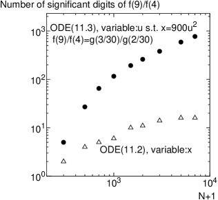
Figure 5: Comparison of the number of significant digits of the ratio $f(9)/f(4)$ between ODE (46) and ODE (47)

In the following, we will give the second example, for the Fuchsian-type ODE

$$xf^{\prime\prime}(x)+f^{\prime}(x)+\left(-\frac{x}{4}+(\nu+\frac{\mu+1}{2})-\frac{\mu^{2}}{x}\right)f(x)=0$$ (44)

with nonnegative integers $\mu$ and $\nu$. Since we have the Fuchsian-type ODE for $\phi(x):=x^{-\mu/2}\,e^{x/2}\,f(x)$

$$x\phi^{\prime\prime}(x)+(\mu+1-x)\phi^{\prime}(x)+\nu f(x)=0$$

which is the associate Laguerre differential equation, it is easily shown that the solutions in $L_{(k_{0})}^{2}(\mathbb{R})$ are proportional to the weighted associate Laguerre function

$$f(x)=\left\{\begin{array}[]{@{\,}ll}C\,x^{\mu/2}\,e^{-x/2}L_{\nu}^{\mu}(x)&(x\geq 0)\\ 0&(x<0)\end{array}\right.\hskip 14.22636pt(C\in\mathbb{R})$$

with the associate Laguerre polynomial $L_{\nu}^{\mu}(x)$. From the last discussion in Section 2, the ODE (44) can be treated by our algorithm as the Fuchsian-type ODE

$$x^{2}f^{\prime\prime}(x)+xf^{\prime}(x)+\left(-\frac{x^{2}}{4}+(\nu+\frac{\mu+1}{2})x-\mu^{2}\right)f(x)=0$$ (46)

whose coefficient functions are polynomials. In this ODE, the polynomial $p_{2}(x)=x^{2}$ of the highest order term has zero point at $x=0$. However, as has been found in many other Fuchsian-type ODEs, numerical results always converge to true solutions empirically. So is this case, and here we show how the results converge to true solutions in this case.

In Fig 5, the results with $\mu=4$, $\nu=3$, $k_{0}=0$, $N+1=200,500$,

$K=2\lfloor\frac{3N}{8}\rfloor+k_{0}$ and $J=2\lfloor\frac{7N}{16}\rfloor+k_{0}$ are shown, under the normalization

$\langle f,\frac{1}{2\pi}(\psi_{k_{0},0}+\psi_{k_{0},-k_{0}-1})\rangle_{{\cal H}}=1$. The error of the result with $N+1=500$ is almost invisible there. It is remarkable that the obtained numerical results are very close to zero for $x<0$ even though the basis functions are not small for $x<0$, though a small oscillation is observed in the result with $N+1=200$. However, the convergence in this case is less rapid than the ODEs without zero points of $p_{M}(x)$, because of the singularity of the solution at $x=0$ where the solutions are not $(\mu/2+1)$-th order differentiable.

To avoid this problem, instead of ODE (44), we solve the ODE

$$u^{2}g^{\prime\prime}(u)+ug^{\prime}(u)+\left(-c^{4}u^{4}+c^{2}(4\nu+2\mu+2)u^{2}-\mu^{2}\right)g(u)=0$$ (47)

with a positive constant $c$, which is derived directly from (44) by the change of coordinate $x=(cu)^{2}$ (where $g(u):=f\left((cu)^{2}\right)$. By this change of coordinate, we can obtain the solutions only for $x\geq 0$, which causes no inconvenience because the true solutions are zero for $x<0$. By this change of coordinate, the accuracy of the numerical result improves drastically, as is shown in Fig. 5 where the number of significant digits of the ratio $\displaystyle\frac{f(9)}{f(4)}$ are compared between the ODEs (46) and (47) with $c=30$. As is shown in this figure, the number of significant digits empirically increases as a power of $N$ for $N+1>10^{3}$ in the case of ODE (47), while it increases approximately proportional to $\log N$ due to the singularity at $x=0$ in the case of (46). The bad behavior for ODE (46) is theoretically deduced also from the fact that the order of coefficient $f_{n}$ in the expansion $f(x)=\sum_{n}f_{n}e_{n}(x)$ is an inverse power of $N$ for a function $f(x)$ with a singularity of this type, in a similar way to the case of Fourier series. The above change of coordinate eliminates this singularity, and it is successful in improving the accuracy to a great extent, up to several hundred digits, as is shown in Figure 5. Moreover, the number of significant digits increases almost in a power of $N$ when $N+1\geq 2000$. This implies that the amount of required calculations increases almost in a polynomial order of the number of required significant digits, from the reasons shown in Subsection 11.2 below.

11.2 Theoretical comparison with existing methods

In this subsection, we compare theoretically the order of the amount of calculations required for a very high accuracy, between some typical existing methods with arbitrary-precision arithmetic and the proposed method. The comparison is made with the following three methods:

(a) Runge-Kutta methods with arbitrary-precision arithmetic.

(b) Finite element methods with arbitrary-precision arithmetic.

(c) Petrov-Galerkin method with arbitrary-precision arithmetic using the same globally smooth basis functions as this paper.

In the following, we compare them for the case where we require $Q$ significant digits for the ratio $f(x_{1})/f(x_{0})$ between the values of a solution function at two points $x_{0}$ and $x_{1}$.

Order of amount of required calculations in the proposed method

The amount of required calculations in the proposed method is almost a power of $Q$ when $Q$ is very large, because it requires about $O(N^{3}(\log N)^{2})$ as was explained in Section 5 (after Theorem 5.2) and many numerical resuts show that $Q$ is almost proportional to a power of $N$ when $N$ is very large. Empirically the amount of required calculations is from $O(Q^{3})$ to $O(Q^{5})$ in many cases. (Moreover, from the discussion in Section 5, we may redice it to be from $O(Q^{2})$ to $O(Q^{4})$ by means of the modification proposed after Theorem 5.2.)

Comparison with (a) Runge-Kutta methods

As is shown in the followong, Method (a) requires more than an exponential order of $Q$. As is known well, the discretization error of the Runge-Kutta methods is proportional to a power $h^{p}$ $(p\geq 4)$ of the step size $h$ for the discretization of the coordinate. (For example, in the common Runge-Kutta method, proportional to $h^{4}$.) This implies that the step size $h$ should satisfy the inequality $C_{0}h^{p}<10^{-Q}$ with a positive constant $C_{0}$. This inequality implies the inequality $\displaystyle\log h<-\frac{\log 10}{p}Q+C_{1}$ with another constant $C_{1}$. Since the numbers $n_{s}$ of the steps between $x_{0}$ and $x_{1}$ is $\displaystyle\frac{|x_{0}-x_{1}|}{h}$, the number of required steps $n_{s}$ should satisfy the inequality $\displaystyle\log n_{s}>\frac{\log 10}{p}Q+C_{2}$ with another constant $C_{2}$. Hence, $\displaystyle n_{s}>C_{3}\,(10)^{\frac{Q}{p}}$ with a positive constant $C_{3}$. Moreover, the number of required digits for the working precision is larger as $Q$ is larger. (At least, it should be larger than $Q$.)   These fact implies that the amount of required calculations is at least $\displaystyle O(Q^{2}\cdot(10)^{\frac{Q}{p}})$. Can you imagine how huge is the amount when $Q$ is several hundreds or several thousands? Hence, the proposed method requires a much smaller amount of calculation than the Runge-Kutta methods, for a very high accuracy.

Comparison with (b) finite element methods

As is shown in the following, also Method (b) requires more than an exponential order of $Q$. As is known well, the error due to finite-dimensional approximation in the finite element methods is proportional to a power of the support size of the finite elements, at least. For example, when the basis functions are piece-wise polynomials of degree $q$ with support size $d$, the error is approximately proportional to $d^{\,q+1}$ at least, which is easily shown by the Taylor expansions of the true solution $f(x)$. Since the required dimension of the subspace is proportional to $\displaystyle\frac{|x_{0}-x_{1}|}{d}$ and the matrix is band-diagonal, from a discussion very similar to the above Runge-Kutta cases, the amount of required calculations is at least $\displaystyle O(Q^{2}\cdot(10)^{\frac{Q}{q+1}})$. This will be huge when $Q$ is very large. Hence, the proposed method requires a much smaller amount of calculation than the finite element methods, for a very high accuracy.

Comparison with (c) Galerkin methods using globally smooth basis functions

For Method (c), since the direct order comparison is difficult, here we only point out that it requires a very large amount of calculations. Let $W$ be the number of required digits for the working precision, and $N+1$ be the dimension of the subspace. Then, since the matrix is band-diagonal, the amount of required calculations is $O(W^{2}N)$. (If we use fast multiplication algorithms, the Karatsuba algorithm for example, the order may decrease to some extent. However, in our numerical examples, we did not use such algorithms. If we use such algorithms, we can diminish the order to the same extent as that. Therefore, for simplicity, here we compare the order without such algorithms.)

In Method (c), it is very difficult to calculate the eigenvector in a high accuracy because of a heavy ‘cancelling’ due to round-off errors, by the following reason, even if the exact eigenvalue is known. In this method, the matrix is band-diagonal with band width $2\ell_{0}+1$ [4]. When we calculate the elements $f_{n}$ ($n=0,1,\ldots,N)$ of the solution vector $\vec{f}$, with unknown intial values $f_{0},f_{1},\ldots f_{\ell_{0}-1}$, we should determine these initial values so that the linear equations given by the bottom $\ell_{0}$ rows of the matrix can be satisfied. This problem can be reduced a system of $\ell_{0}$ inhomogeneous simultaneous linear equation represented by a $\ell_{0}\times\ell_{0}$ matrix.

However, this $\ell_{0}\times\ell_{0}$ matrix is usually very close to a singular matrix of rank 1, because of the most diverging component contained in the halfway of the calculations of $f_{n}$ ($n=\ell_{0},\ell_{0}+1,\ldots N-\ell_{0}$). In other words, with whatever initial values, the vector obtained in the halfway of the calculation are almost parallel to this diverging component, because this diverging component is dominant. Moreover, that $\ell_{0}\times\ell_{0}$ matrix is more close to a singular matrix of rank 1, as the dimension $N+1$ is larger.

Though the order of this approach is difficult to estimate because it depends on the differential equation, anyway we should choose $W$ so that $\displaystyle\frac{W}{(\ell_{0}-1)Q}$ can be much larger than a monotonously increasing function of $N$ not smaller than $1$, in order to avoid the above mentioned ‘cancelling’. The total order estimation of this case and the comparison with the proposed method is one of future problem.

Even if we use other methods for the calculation of the eigenvector, the Gaussian elimination or the diagonalization for example, the basic mathematical structure is the same as the above, and the problem due to the closeness to a linear dependence arises there.

Even if we use the Galerkin methods using another type of globally smooth basis functions, the Hermite functions for example, the basic circumstance is still similar to this.

Thus, the proposed method requires a much smaller amount of calculations than Runge-Kutta and finite element methods, in order to calculate the values of the solution function $f(x)$ at a finite number of points in an extraordinarily high accuracy. This is the reason why we have many nurerical results by ordinary personal computers where $Q$ is so large as several hundreds or several thousands.

12 Conclusions

We have explained how to realize the integer-type algorithm proposed in [4] for linear higher-order differential equations, and proved that the realization proposed there satisfies the conditions given in C7 which are required for the convergence of numerical results to the true ‘general solutions’ in ${\cal H}$ of the differential equations.

We have proved that the method based on quasi-orthogonalization can obtain vectors in the quasi-optimal set $(\sigma_{K,N}^{(\Omega)})^{-1}[0,c\underline{\sigma_{K,N}^{(\Omega)}}]$ with fixed $c$. Moreover, we have provided some proofs about the extension for the case with $\dim V\cap\ell^{2}(\mathbb{Z}^{+})\geq 2$ and the halting of the procedures.

In addition, we have given a theoretical upper bound for the errors as a function only of the worst truncation error, in terms of one unknown parameter $\Delta_{K}$ (the worst truncation error of the exact true solutions).

Numerical results have shown the precision of the proposed method. In addition, we have given an example which attains the exact ratios among the coefficients $f_{n}$ in the expansion $f(x)=\sum_{n}f_{n}e_{n}(x)$.

In the near future, we will compare the norm of actual errors in numerical results and the upper bound proposed in this paper, and investigate the tightness of this upper bound. Remaining problems include improvements of the algorithm to reduce the number of calculations and better choices of the bilinear form $Q(\vec{f},\vec{g})$, and the orthogonality parameters $h$ and $g$.

Appendix A Other orthogonality-like relations for $\psi_{k,n}$

With respect to the usual $L^{2}$-inner product

$$(f,\,g):=\int_{-\infty}^{\infty}f(x)\,\overline{g(x)}\,dx\,\,,$$

the orthogonality-like relation

$$(\psi_{k,\,n},\psi_{k,\,n^{\prime}})=\left\{\begin{array}[]{@{\,}ll}\displaystyle\frac{\pi}{4^{k}}\,\,(-1)^{n-n^{\prime}}\frac{(2k)!}{(k+n-n^{\prime})!\,\,(k+n^{\prime}-n)!}&(\,|n-n^{\prime}|\leq k\,)\\ \\ \displaystyle 0&({\rm otherwise})\end{array}\right.$$

holds. With respect to another inner product

$$\langle f,\,g\rangle_{|D|^{-k}}:=\int_{-\infty}^{\infty}({\cal F}f)(y)\,\overline{({\cal F}g)(y)}\,\,\frac{dy}{|y|^{k}}$$

(where ${\cal F}$ denotes the operator of Fourier transformation), another type of

orthogonality-like relation

$${}^{\forall}n,\,n^{\prime}\in\mathbb{Z}^{+},\,\,\,\,\,\,\,\,\langle\psi_{k,\,n},\psi_{k,\,n^{\prime}}\rangle_{|D|^{-k}}=\frac{\pi}{16^{k}}\,\frac{n!}{(n+2k)!}\,\,\delta_{nn^{\prime}}$$

holds. This relation is derived from the orthogonality of the number states associated with the algebra $\mathfrak{su}(1,1)$  [11]. Here note that $\langle f,\,g\rangle_{(0)}=\langle f,\,g\rangle_{|D|^{-0}}=(f,\,g)$.

Appendix B On the shape of the wavepackets $\psi_{k,\,n}(x)$

The wavepackets are complex-valued ‘wavy’ functions. By the scale change $x\to x/\sqrt{k}$, the ‘envelope’ function

$$|\psi_{k,n}(x)|=(x^{2}+1)^{-\frac{k+1}{2}}$$ (49)

of the wavepacket $\psi_{k,\,n}^{(}x)$ is proportional to the probability density function of the (Student) $t$-distribution with the degree of freedom $k$ (used in statistics), which tends to the standard Gaussian function as $k\to\infty$. Since the ‘foot of the mountain’ of the probability density function of the $t$-distribution is thicker when $k$ is smaller, the ‘localization’ of the envelope of the wavepacket is better as $k$ becomes larger when a comparison is made with respect to the normalized ‘width’ (or standard deviation). The ‘phase’ function of the wavepacket is

$$\arg\,\psi_{k,\,n}(x)=(k+2n+1)\,\,(\arctan x-\frac{\pi}{2})\,.$$ (50)

This function is almost linear when $|x|$ is not too large (because then $\arctan x\approx x$), and we can approximate the wavepacket by a sinusoidal wavepacket with the above envelope function, because the envelope function is sufficiently small where the phase function deviates considerably from the linear function $(k+2n+1)\,(x-\frac{\pi}{2})$. This approximate picture is very good especially in the cases with large $k$ though it is poor for the cases with small $k$, because the ‘foot of the mountain’ of the envelope vanishes very rapidly for large $k$. In fact, for sufficiently large $k$,

$$\psi_{k,n}(x)\approx(-i)^{k+2n+1}\,\,\,e^{i(k+2n+1)x}\,\,\,(x^{2}+1)^{-\frac{k+1}{2}}$$

$${\rm or}\,\,\,\,\,\,\,\,\,\,\,\,\psi_{k,n}(x)\approx{\textstyle\frac{\sqrt{k\pi}\,\Gamma(\frac{k}{2})}{\Gamma({\frac{k+1}{2})}}}\,\,\,e^{i(k+2n+1)x}\,\,\,e^{-\frac{k}{2}x^{2}}\,\,\,.$$

For this, we can prove easily that the function $\displaystyle\,\Xi_{k}\,e^{-i\xi_{k,n}x}\,\psi_{k,n}(\frac{x}{\sqrt{k}})\,\,$ with

$\displaystyle\Xi_{k}:=\frac{\Gamma({\frac{k+1}{2})}}{\pi\sqrt{2k}\,\Gamma(\frac{k}{2})}$ and $\displaystyle\xi_{k,n}:=\frac{k+2n+1}{\sqrt{k}}\,$ converges to the standard Gaussian function

$\displaystyle\frac{1}{\sqrt{2\pi}}\,e^{-\frac{1}{2}x^{2}}$ as $k\to\infty$ for the $L^{2}$-norm, by means of the upper and lower bounds of the Stirling formula, because the properties (49) and (50) lead us to

$$\Xi_{k}\,e^{-i\,\xi_{k,n}x}\,\psi_{k,n}(\frac{x}{\sqrt{k}})-\frac{1}{\sqrt{2\pi}}\,e^{-\frac{1}{2}x^{2}}$$

$$=\frac{1}{\sqrt{2\pi}}\,\left(e^{-i\,(k+2n+1)\bigl{(}\frac{x}{\sqrt{k}}\,-\,\arctan\frac{x}{\sqrt{k}}\bigr{)}}\,\sqrt{\frac{2\pi\,\,\Xi_{k}^{2}\,\,e^{x^{2}}}{\displaystyle\bigl{(}1+\frac{x^{2}}{k}\bigr{)}^{k+1}}}\,\,-\,\,1\,\right)\,e^{-\frac{1}{2}x^{2}}.$$

This picture of the wavepackets, ‘almost-sinusoidal’ oscillations with a spindle-shaped envelope, which are similar to Gaussian-weighted (complex) sinusoidal

wavepackets, is ‘natural’ and useful in many applications, and it is very convenient for the interpretation of the basis systems used in this paper (for this, the relationship between these wavepackets and the Fourier series is shown in Appendix B of  [5]).

References

- [1] E. A. Coddington and N. Levinson, Theory of Ordinary Differential Equations, McGraw-Hill, New York (1955).
- [2] M. A. Krasnosel’slii, G. M. Vainikko, P. P. Zabreiko, Y. B. R. Utitskii, and V/Y. Stetsenko, Approximate Solution of Operator Equations, translated by D. Louvish, Wolters-Noordhoff Publishing, Groningen (1972).
- [3] S. C. Brenner, The Mathematical Theory of Finite Element Methods, Springer, New York (2007).
- [4] F. Sakaguchi and M. Hayashi, General theoty for integer-type algorithm for higher order differential equations, arXiv:0903.4848.
- [5] F. Sakaguchi and M. Hayashi, Differentiability of eigenfunctions of the closures of differential operators with rational coefficient functions, arXiv:0903.4852.
- [6] A. W. Eldély et al, Higher transcendental functions, 3 vols., McGraw-Hill, New York (1953-55).
- [7] T. Qian et al., Analytic unit quadrature signals with nonlinear phase, Physica D, 203, 80-87 (2005).
- [8] Q. Chen et el., Two families of unit analytic signals with nonlinear phase, Physica D, 221, 1-12 (2006).
- [9] A. K. Lenstra, H. W. Lenstra Jr and L. Lovász, Factoring polynomials with rational coefficients, Math. Ann. 261, 515-534 (1982).
- [10] L. Babai, On Lovász’ lattice reduction and the nearest lattice point problem, Combinatorica, 6(1), 1-13 (1986).
- [11] F. Sakaguchi and M. Hayashi, Coherent states and annihilation-creation operators associated with the irreducible unitary representations of , J. Math. Phys., 43, 2241-2248 (2002).