A fast impurity solver based on equations of motion and decoupling

Abstract

In this paper a fast impurity solver is proposed for dynamical mean field theory (DMFT) based on a decoupling of the equations of motion for the impurity Greens function. The resulting integral equations are solved efficiently with a method based on genetic algorithms. The Hubbard and periodic Anderson models are studied with this impurity solver. The method describes the Mott metal insulator transition and works for a large range of parameters at finite temperature on the real frequency axis. This makes it useful for the exploration of real materials in the framework of LDA+DMFT.

I Introduction

Understanding exotic physical properties, such as high-T_c superconductivity and the correlation-driven Mott metal-insulator transition of strongly correlated compounds (typically those including $d$ or $f$ electrons), remains a hard and fundamental task in modern condensed matter physics. During the past decade, the development and application of dynamical mean-field theory (DMFT) has led to a considerable improvement in our understanding of these systems. georges96 ; metzner89 ; georges92 . The essence of DMFT is to map a many-electron system to a single impurity atom embedded in a self-consistently determined effective medium by neglecting all the spatial fluctuations of the self-energy. However, this resulting quantum impurity model remains a fully interacting many-body problem that has to be solved, and the success of DMFT depends on the availability of reliable methods for calculation of the local self-energy of the impurity model.

Accordingly, much effort has been devoted to develop various impurity solvers. Among those, the iterated perturbation theory (IPT) georges92 ; Zhang ; Kajueter ; Fujiwara , the non-crossing approximation (NCA) Keiter ; Grewe ; Kuramoto ; Haule , equation-of-motion (EOM) method jeschke05 ; zhu05 ; qi08 , Hubbard I approximation (HIA) Hubbard , fluctuation exchange (FLEX) approximation Chioncel ; Drchal , the quantum Monte Carlo method (Hirsch-Fye algorithm) (HF-QMC) Hirsch ; Jarrell ; Georges ; Rozenberg , the continuous time quantum Monte Carlo method (CTQMC) Werner ; Rubtsov , the exact diagonalization (ED) Caffarel ; Si , the numerical renormalization group (NRG) method Bulla1 ; Bulla2 , and the density matrix renormalization group (DMRG) method Garcia ; karski08 are widely adopted. However, every impurity solver has its own limitation. IPT originally cannot be applied to the case away from half-filling while a modified IPT which can solve this problem has to introduce an ansatz to interpolate the weak and strong coupling limits, and the generalization of IPT to the multi-orbital case requires more assumptions and approximations. NCA cannot yield the Fermi liquid behavior at low energies and in the low temperature limit. The HIA can only be applied to strongly localized electron systems like $f$ electrons. FLEX works well in the metallic region while it fails in the large $U$ region. Before the appearance of CTQMC, the HF-QMC was not applicable in the low temperature limit and has serious difficulties in application to multi-orbital systems with spin-flip and pair-hopping terms of the exchange interaction since the Hubbard-Stratonovich transformation Held cannot be performed in these systems. But even for CTQMC, the requirement to do analytical continuation of the results to the real frequency axis remains, which introduces some uncertainty especially for multi-orbital systems. In the ED method, an additional procedure is required for the discretization of the bath and as a consequence, the method is unable to resolve low-energy features at the Fermi level. NRG aims at a very precise description of the low-frequency quasiparticle peaks associated with low-energy excitations while it has less precision in the Hubbard bands which are important in calculating the optical conductivity. Furthermore, all the numerically exact impurity solvers QMC, ED, NRG and DMRG are computationally expensive.

However, today, a fast and reliable impurity solver is really urgently needed due to the fact that great achievements have been made in understanding correctly the strongly correlated systems from first principle by combining DMFT and local density approximation (LDA) in density functional theory (DFT), so called LDA+DMFT Kotliar . The aim of this paper is to present a fast and reliable impurity solver based on the EOM method. Equation of motion methods are limited by their decoupling scheme, but EOM has shown its value by working directly on the real frequency axis and at very low temperature. It can be a good candidate for a faster and reliable impurity solver by choosing a suitable decoupling scheme. In fact, the infinite $U$ case was studied by the EOM method for Hubbard model, periodic Anderson model and $pd$ model in Ref. jeschke05, . In Ref. zhu05, , the finite $U$ case is studied without calculating the physical quantities self-consistently. Recently qi08 , this method has been improved by taking into account selfconsistency and applied to the Anderson impurity model in the large-$N$ limit. The operator projection method (OPM) Onoda01 is related to the EOM method. In this paper, we will use a different decoupling procedure than used previously for a set of EOMs of the Anderson impurity model and then apply this new impurity solver to the finite $U$ Hubbard model as well as periodic Anderson model via dynamical mean field theory. Meanwhile, we employ genetic algorithms to efficiently search for the self-consistent solution. The genetic algorithm significantly reduces the CPU time for convergence and improves the energy resolution in the DMFT calculation.

The paper is organized as follows: In Section II we present the EOMs we use and introduce our decoupling scheme. In Section III we describe how the genetic algorithm is implemented in our DMFT loop. Finally, in Section IV we test our EOM impurity solver on the Hubbard model and periodic Anderson model.

II Equations of motion and decoupling procedure

We start with the Hamiltonian of the single impurity Anderson model. For arbitrary degeneracy $N$, it is given by

$${\cal H} = \sum_{k\sigma}\varepsilon_{k}c^{{\dagger}}_{k\sigma}c_{k\sigma}+\sum_{\sigma}\varepsilon_{f}f^{{\dagger}}_{\sigma}f_{\sigma}+\frac{U}{2}\sum_{\sigma\sigma^{\prime}}\hat{n}_{\sigma}\hat{n}_{\sigma^{\prime}}$$ (1)

$$\qquad\qquad+\sum_{k\sigma}\big{(}V^{\ast}_{k\sigma}c^{{\dagger}}_{k\sigma}f_{\sigma}+V_{k\sigma}f^{{\dagger}}_{\sigma}c_{k\sigma}\big{)}$$

where $c^{{\dagger}}_{k\sigma}$, $c_{k\sigma}$, $f^{{\dagger}}_{\sigma}$ and $f_{\sigma}$ are the creation and annihilation operators for the conduction electrons and for the correlated impurity electrons, respectively. $\hat{n}_{\sigma}=f^{{\dagger}}_{\sigma}f_{\sigma}$ corresponds to the density of the $f$ electrons. $\varepsilon_{k}$ is the dispersion of the conduction electrons, $\varepsilon_{f}$ is the site energy of the correlated electron, $U$ is the on-site Coulomb interaction strength of the $f$ electrons, and $V_{k\sigma}$ is hybridization between conduction and correlated electrons.

In studying the system described by the Hamiltonian of Eq. 1, we consider the double time temperature-dependent retarded Greens function in Zubarev notation zubarev60 ,

$$G_{AB}(t,t^{\prime})={\langle\!\langle}A(t);B(t^{\prime}){\rangle\!\rangle}=-i\Theta(t-t^{\prime})\langle[A(t),B(t^{\prime})]_{+}\rangle$$ (2)

involving the two Heisenberg operators $A(t)$ and $B(t^{\prime})$. It is convenient to work with the Fourier transform, which is defined as

$${\langle\!\langle}A;B{\rangle\!\rangle}_{\omega}=\int^{\infty}_{-\infty}dte^{i\omega(t-t^{\prime})}{\langle\!\langle}A(t);B(t^{\prime}){\rangle\!\rangle}\,.$$ (3)

In the framework of the equation of motion method, the Greens function should satisfy the equation of motion

$$\omega{\langle\!\langle}A;B{\rangle\!\rangle}=\langle[A,B]_{+}\rangle+{\langle\!\langle}[A,{\cal H}];B{\rangle\!\rangle}$$ (4)

where we have neglected the lower indices $\omega$. In the following, all the Greens functions depend on frequency $\omega$.

As a result of the coupling between conduction and $f$ electrons, we find the equations of motion,

$$(\omega-\varepsilon_{d}-\Delta){\langle\!\langle}f_{\sigma};f^{{\dagger}}_{\sigma}{\rangle\!\rangle} = 1+(N-1)U{\langle\!\langle}\hat{n}_{\sigma^{\prime}}f_{\sigma};f^{{\dagger}}_{\sigma}{\rangle\!\rangle}_{\sigma\neq\sigma^{\prime}}$$ (5)

$$(\omega-\varepsilon_{d}-U){\langle\!\langle}\hat{n}_{\sigma^{\prime}}f_{\sigma};f^{{\dagger}}_{\sigma}{\rangle\!\rangle} = \bar{n}_{\sigma^{\prime}}+(N-2)U{\langle\!\langle}\hat{n}_{\sigma^{\prime\prime}}\hat{n}_{\sigma^{\prime}}f_{\sigma};f^{{\dagger}}_{\sigma}{\rangle\!\rangle}+\sum_{k}(-V^{*}_{k\sigma^{\prime}}{\langle\!\langle}c^{{\dagger}}_{k\sigma^{\prime}}f_{\sigma^{\prime}}f_{\sigma};f^{{\dagger}}_{\sigma}{\rangle\!\rangle}$$ (6)

$$+V_{k\sigma}{\langle\!\langle}\hat{n}_{\sigma^{\prime}}c_{k\sigma};f^{{\dagger}}_{\sigma}{\rangle\!\rangle}+V_{k\sigma^{\prime}}{\langle\!\langle}f^{{\dagger}}_{\sigma^{\prime}}c_{k\sigma^{\prime}}f_{\sigma};f^{{\dagger}}_{\sigma}{\rangle\!\rangle})$$

$$(\omega-\varepsilon_{k}){\langle\!\langle}\hat{n}_{\sigma^{\prime}}c_{k\sigma};f^{{\dagger}}_{\sigma}{\rangle\!\rangle} = V^{*}_{k\sigma}{\langle\!\langle}\hat{n}_{\sigma^{\prime}}f_{\sigma};f^{{\dagger}}_{\sigma}{\rangle\!\rangle}+\sum_{k^{\prime}}(-V^{*}_{k^{\prime}\sigma^{\prime}}{\langle\!\langle}c^{{\dagger}}_{k^{\prime}\sigma^{\prime}}f_{\sigma^{\prime}}c_{k\sigma};f^{{\dagger}}_{\sigma}{\rangle\!\rangle}+V_{k^{\prime}\sigma^{\prime}}{\langle\!\langle}f^{{\dagger}}_{\sigma^{\prime}}c_{k^{\prime}\sigma^{\prime}}c_{k\sigma};f^{{\dagger}}_{\sigma}{\rangle\!\rangle})$$ (7)

$$(\omega-\varepsilon_{k}){\langle\!\langle}f^{{\dagger}}_{\sigma^{\prime}}c_{k\sigma^{\prime}}f_{\sigma};f^{{\dagger}}_{\sigma}{\rangle\!\rangle} = \langle f^{{\dagger}}_{\sigma^{\prime}}c_{k\sigma^{\prime}}\rangle+V^{*}_{k\sigma^{\prime}}{\langle\!\langle}\hat{n}_{\sigma^{\prime}}f_{\sigma};f^{{\dagger}}_{\sigma}{\rangle\!\rangle}+\sum_{k^{\prime}}(-V^{*}_{k^{\prime}\sigma^{\prime}}{\langle\!\langle}c^{{\dagger}}_{k^{\prime}\sigma^{\prime}}c_{k\sigma^{\prime}}f_{\sigma};f^{{\dagger}}_{\sigma}{\rangle\!\rangle}$$ (8)

$$+V_{k^{\prime}\sigma}{\langle\!\langle}f^{{\dagger}}_{\sigma^{\prime}}c_{k\sigma^{\prime}}c_{k^{\prime}\sigma};f^{{\dagger}}_{\sigma}{\rangle\!\rangle})$$

$$(\omega+\varepsilon_{k}-2\varepsilon_{d}-U){\langle\!\langle}c^{{\dagger}}_{k\sigma^{\prime}}f_{\sigma^{\prime}}f_{\sigma};f^{{\dagger}}_{\sigma}{\rangle\!\rangle} = \langle c^{{\dagger}}_{k\sigma^{\prime}}f_{\sigma^{\prime}}\rangle+2(N-2)U{\langle\!\langle}c^{{\dagger}}_{k\sigma^{\prime}}\hat{n}_{\zeta}f_{\sigma^{\prime}}f_{\sigma};f^{{\dagger}}_{\sigma}{\rangle\!\rangle}_{\begin{subarray}{c}\zeta\neq\sigma\\ \zeta\neq\sigma^{\prime}\end{subarray}}-V_{k\sigma^{\prime}}{\langle\!\langle}f^{{\dagger}}_{\sigma^{\prime}}f_{\sigma^{\prime}}f_{\sigma};f^{{\dagger}}_{\sigma}{\rangle\!\rangle}$$ (9)

$$+\sum_{k^{\prime}}(V_{k^{\prime}\sigma}{\langle\!\langle}c^{{\dagger}}_{k\sigma^{\prime}}f_{\sigma^{\prime}}c_{k^{\prime}\sigma};f^{{\dagger}}_{\sigma}{\rangle\!\rangle}+V_{k^{\prime}\sigma^{\prime}}{\langle\!\langle}c^{{\dagger}}_{k\sigma^{\prime}}c_{k^{\prime}\sigma^{\prime}}f_{\sigma};f^{{\dagger}}_{\sigma}{\rangle\!\rangle})$$

where $\Delta(\omega)=\sum_{k}\frac{V^{\ast}_{k\sigma}V_{k\sigma}}{\omega-\varepsilon_{k}}$ is the hybridization function and we have used

$$(\omega-\varepsilon_{k}){\langle\!\langle}c_{k\sigma};f^{{\dagger}}_{\sigma}{\rangle\!\rangle}=V^{\ast}_{k\sigma}{\langle\!\langle}f_{\sigma};f^{{\dagger}}_{\sigma}{\rangle\!\rangle}\,.$$ (10)

These equations are generalized to arbitrary degeneracy $N$ compared to Ref. lacroix81, , i.e. they are at the same level as Ref. czycholl85, . Now a decoupling scheme is needed to truncate the equations of motion in order to get a closed set of equations. Here we have used the cluster expansion scheme proposed in Ref. wang94, where the higher order Greens functions are separated into connected Greens functions of the same order and lower order Greens functions. The connected Greens function can not be decoupled any further as defined. This expansion scheme gives a natural and systematical way for truncation. It has been used in Ref. luo99, for studying the single impurity Anderson model, in particular for infinite interaction strength $U$. This approach to decoupling could be used to study the EOM method beyond the level of Ref. lacroix82, . The detailed cluster expansion scheme is given as

$${\langle\!\langle}1;2{\rangle\!\rangle} = {\langle\!\langle}1;2{\rangle\!\rangle}_{c}$$ (11)

$${\langle\!\langle}123;4{\rangle\!\rangle} = {\langle\!\langle}123;4{\rangle\!\rangle}_{c}+{\hat{A}s}_{(2,3)}\langle 12\rangle{\langle\!\langle}3;4{\rangle\!\rangle}$$ (12)

$${\langle\!\langle}12345;6{\rangle\!\rangle} = {\langle\!\langle}12345;6{\rangle\!\rangle}_{c}$$ (13)

$$+ {\hat{A}s}_{(2,4,5)}{\hat{S}p}_{(1,2;3,4)}\big{(}\langle 12\rangle\langle 34\rangle{\langle\!\langle}5;6{\rangle\!\rangle}$$

$$+ \langle 1234\rangle_{c}{\langle\!\langle}5;6{\rangle\!\rangle}+\langle 12\rangle{\langle\!\langle}345;6{\rangle\!\rangle}_{c}\big{)}~{}~{}~{}~{}~{}$$

where digits 1-6 stand for operators, $\hat{A}s_{(i,j,k)}$ is the antisymmetrization operator for operators $(ijk)$, $\hat{S}p_{(1,2;3,4)}$ is the symmetrization operator for pair exchange between $(1,2)$ and $(3,4)$, and Greens functions or correlations marked by an index $c$ represent connected terms.

Using this decoupling scheme and neglecting all the three-particle connected Greens functions and those two-particle connected Greens functions which involve two $c$ operators, i.e. ${\langle\!\langle}c^{+}_{k\sigma^{\prime}}c_{k^{\prime}\sigma^{\prime}}f_{\sigma};f^{{\dagger}}_{\sigma}{\rangle\!\rangle}_{c}$, ${\langle\!\langle}c^{+}_{k\sigma^{\prime}}f_{\sigma^{\prime}}c_{k^{\prime}\sigma};f^{{\dagger}}_{\sigma}{\rangle\!\rangle}_{c}$ etc., and by assuming correlations with spin flip to be zero, e.g. $\langle f^{{\dagger}}_{\sigma^{\prime}}f_{\sigma}\rangle=0$, we can get the single electron Greens function for arbitrary degeneracy $N$ at the level of approximation of Ref. lacroix82, as

$$(\omega-\varepsilon_{d}-\Delta-AB){\langle\!\langle}f_{\sigma};f^{{\dagger}}_{\sigma}{\rangle\!\rangle}=1+A\big{\{}\bar{n}_{\sigma^{\prime}}+C\big{\}}$$ (14)

where

$$A = \frac{(N-1)U}{\omega-\varepsilon_{d}-U-(N-2)U\bar{n}_{\sigma^{\prime\prime}}-2\Delta-\tilde{\Delta}}$$ (15)

$$B = \bigg{[}(N-2)U\langle\hat{n}_{\sigma^{\prime\prime}}\hat{n}_{\sigma^{\prime}}\rangle_{c}+\sum_{k,k^{\prime}}\Big{(}-\frac{V_{k\sigma^{\prime}}V^{*}_{k^{\prime}\sigma^{\prime}}\langle c^{+}_{k^{\prime}\sigma^{\prime}}c_{k\sigma^{\prime}}\rangle}{\omega-\varepsilon_{k}}$$ (16)

$$+\frac{V_{k\sigma^{\prime}}V_{k^{\prime}\sigma}V^{*}_{k^{\prime}\sigma}}{(\omega-\varepsilon_{k})(\omega-\varepsilon_{k^{\prime}})}\langle f^{{\dagger}}_{\sigma^{\prime}}c_{k\sigma^{\prime}}\rangle\Big{)}$$

$$- \sum_{k}\frac{2(N-2)U\langle\hat{n}_{\sigma^{\prime\prime}}c^{+}_{k\sigma^{\prime}}f_{\sigma^{\prime}}\rangle_{c}}{\omega+\varepsilon_{k}-2\varepsilon_{d}-U-2(N-2)U\bar{n}_{\sigma^{\prime\prime}}}$$

$$- \sum_{k}\frac{V^{*}_{k\sigma^{\prime}}\sum_{k^{\prime}}(\frac{V_{k^{\prime}\sigma}V^{*}_{k^{\prime}\sigma}}{\omega-\varepsilon_{k^{\prime}}}\langle c^{+}_{k\sigma^{\prime}}f_{\sigma^{\prime}}\rangle+V_{k^{\prime}\sigma^{\prime}}\langle c^{+}_{k\sigma^{\prime}}c_{k^{\prime}\sigma^{\prime}}\rangle)}{\omega+\varepsilon_{k}-2\varepsilon_{d}-U-2(N-2)U\bar{n}_{\sigma^{\prime\prime}}}\bigg{]}~{}~{}~{}~{}~{}$$

$$C = \sum_{k}\Big{(}\frac{V_{k\sigma^{\prime}}\langle f^{{\dagger}}_{\sigma^{\prime}}c_{k\sigma^{\prime}}\rangle}{\omega-\varepsilon_{k}}$$ (17)

$$-\frac{V^{*}_{k\sigma^{\prime}}\langle c^{+}_{k\sigma^{\prime}}f_{\sigma^{\prime}}\rangle}{\omega+\varepsilon_{k}-2\varepsilon_{d}-U-2(N-2)U\bar{n}_{\sigma^{\prime\prime}}}\Big{)}~{}~{}~{}~{}~{}$$

$$\tilde{\Delta} = \sum_{k}\frac{V^{*}_{k\sigma^{\prime}}V_{k\sigma^{\prime}}}{\omega+\varepsilon_{k}-2\varepsilon_{d}-U-2(N-2)U\bar{n}_{\sigma^{\prime\prime}}}$$ (18)

in which $\bar{n}_{\sigma^{\prime}}=\langle\hat{n}_{\sigma^{\prime}}\rangle$. This set of equations (14)-(18) is closed by the following two equations for the two-particle connected correlations:

$$\begin{split}&\langle\hat{n}_{\sigma^{\prime\prime}}\hat{n}_{\sigma^{\prime}}\rangle_{c}=-\frac{1}{\pi}\int d(\omega^{\prime})f(\omega^{\prime})\textrm{Im}{\langle\!\langle}\hat{n}_{\sigma^{\prime}}f_{\sigma^{\prime\prime}};f^{{\dagger}}_{\sigma^{\prime\prime}}{\rangle\!\rangle}_{c}=-\frac{1}{\pi}\int d(\omega^{\prime})f(\omega^{\prime})\textrm{Im}({\langle\!\langle}\hat{n}_{\sigma^{\prime}}f_{\sigma^{\prime\prime}};f^{{\dagger}}_{\sigma^{\prime\prime}}{\rangle\!\rangle}-\bar{n}_{\sigma^{\prime}}{\langle\!\langle}f_{\sigma^{\prime\prime}};f^{{\dagger}}_{\sigma^{\prime\prime}}{\rangle\!\rangle})\\ &\langle\hat{n}_{\sigma^{\prime\prime}}c^{+}_{k\sigma^{\prime}}f_{\sigma^{\prime}}\rangle_{c}=-\frac{1}{\pi}\int d(\omega^{\prime})f(\omega^{\prime})\textrm{Im}{\langle\!\langle}c^{{\dagger}}_{\sigma^{\prime}}f_{\sigma^{\prime}}f_{\sigma^{\prime\prime}};f^{{\dagger}}_{\sigma^{\prime\prime}}{\rangle\!\rangle}_{c}=-\frac{1}{\pi}\int d(\omega^{\prime})f(\omega^{\prime})\textrm{Im}({\langle\!\langle}c^{{\dagger}}_{\sigma^{\prime}}f_{\sigma^{\prime}}f_{\sigma^{\prime\prime}};f^{{\dagger}}_{\sigma^{\prime\prime}}{\rangle\!\rangle}-\langle c^{{\dagger}}_{\sigma^{\prime}}f_{\sigma^{\prime}}\rangle{\langle\!\langle}f_{\sigma^{\prime\prime}};f^{{\dagger}}_{\sigma^{\prime\prime}}{\rangle\!\rangle})\end{split}$$

where the two-particle Greens function can be obtained from the single-electron Greens function together with Eq. (5) and Eq. (9). Finally the two connected correlations are

$$\langle\hat{n}_{\sigma^{\prime\prime}}\hat{n}_{\sigma^{\prime}}\rangle_{c} = -\frac{1}{\pi}\int d(\omega)f(\omega)\textrm{Im}\frac{1}{(N-1)U}\big{(}(\omega-\varepsilon_{d}-\Delta-(N-1)U\bar{n}_{\sigma^{\prime}}){\langle\!\langle}f_{\sigma^{\prime\prime}};f^{{\dagger}}_{\sigma^{\prime\prime}}{\rangle\!\rangle}\big{)}$$ (19)

$$\langle\hat{n}_{\sigma^{\prime\prime}}c^{+}_{k\sigma^{\prime}}f_{\sigma^{\prime}}\rangle_{c} = \frac{-\frac{1}{\pi}\int d(\omega)f(\omega)\textrm{Im}\Big{\{}\Big{[}\frac{-\frac{V_{k\sigma^{\prime}}}{(N-1)U}(\omega-\varepsilon_{d}-\Delta)+\Delta\langle c^{{\dagger}}_{k\sigma^{\prime}}f_{\sigma^{\prime}}\rangle+\sum_{k^{\prime}}V_{k^{\prime}\sigma^{\prime}}\langle c^{{\dagger}}_{k\sigma^{\prime}}c_{k^{\prime}\sigma^{\prime}}\rangle}{\omega-\varepsilon_{k}-2\varepsilon_{d}-U-2(N-2)U\bar{n}_{\sigma^{\prime}}}-\langle c^{{\dagger}}_{\sigma^{\prime}}f_{\sigma^{\prime}}\rangle\Big{]}{\langle\!\langle}f_{\sigma^{\prime\prime}};f^{{\dagger}}_{\sigma^{\prime\prime}}{\rangle\!\rangle}+D\Big{\}}}{1-\frac{2(N-2)}{\pi}\int d(\omega)f(\omega)\text{Im}\frac{{\langle\!\langle}f_{\sigma^{\prime\prime}};f^{{\dagger}}_{\sigma^{\prime\prime}}{\rangle\!\rangle}}{\omega-\varepsilon_{k}-2\varepsilon_{d}-U-2(N-2)U\bar{n}_{\sigma^{\prime}}}}~{}~{}~{}~{}$$ (20)

where

$$D=\frac{\frac{V_{k\sigma^{\prime}}}{(N-1)U}+\langle c^{{\dagger}}_{\sigma^{\prime}}f_{\sigma^{\prime}}\rangle}{\omega-\varepsilon_{k}-2\varepsilon_{d}-U-2(N-2)U\bar{n}_{\sigma^{\prime}}}$$ (21)

Compared to Ref. lacroix82, , the set of equations (14)-(18) are generalized to arbitrary degeneracy $N$. Ref. czycholl85, has equations of motion at the same level, but there the three particle Greens functions are neglected in the limit $U\rightarrow\infty$, while the Greens functions involving two $c$ operators are considered to give little contribution for $V\rightarrow 0$. Thus, the decoupling of Ref. czycholl85, is constructed in the limit of parameters $U\rightarrow\infty$, $V\rightarrow 0$. In Ref. luo99, , the single impurity Anderson model is studied for infinite interaction strength $U$ and $N=2$, and the focus is on the approximation beyond that of Ref. lacroix81, with the decoupling scheme of Ref. wang94, . Here we have implemented the system of equations (14)-(18) for finite $U$ with arbitrary degeneracy $N$ while neglecting the two particle connected correlations $\langle\hat{n}_{\sigma^{\prime\prime}}\hat{n}_{\sigma^{\prime}}\rangle_{c}$ and $\langle\hat{n}_{\sigma^{\prime\prime}}c^{+}_{k\sigma^{\prime}}f_{\sigma^{\prime}}\rangle_{c}$.

If we now specialize to degeneracy $N=2$ and use the Hermitian conjugate $\langle f^{{\dagger}}_{\sigma^{\prime}}c_{k\sigma^{\prime}}\rangle=\langle c^{+}_{\sigma^{\prime}}f_{\sigma^{\prime}}\rangle$, the set of equations (14)-(18) becomes

$${\langle\!\langle}f_{\sigma};f^{{\dagger}}_{\sigma}{\rangle\!\rangle}=\frac{1+\frac{U}{\omega-\varepsilon_{d}-U-2\Delta-\tilde{\Delta}}\big{\{}\bar{n}_{\sigma^{\prime}}+I_{1}\big{\}}}{\omega-\varepsilon_{d}-\Delta-\frac{U}{\omega-\varepsilon_{d}-U-2\Delta-\tilde{\Delta}}\big{\{}I_{1}\cdot\Delta+I_{2}\big{\}}}~{}$$ (22)

with

$$I_{1} = \sum_{k}\Big{(}\frac{V_{k\sigma^{\prime}}\langle f^{{\dagger}}_{\sigma^{\prime}}c_{k\sigma^{\prime}}\rangle}{\omega-\varepsilon_{k}}-\frac{V^{\ast}_{k\sigma^{\prime}}\langle f^{{\dagger}}_{\sigma}c_{k\sigma}\rangle}{\omega+\varepsilon_{k}-2\varepsilon_{d}-U}\Big{)}$$ (23)

$$I_{2} = -\sum_{kk^{\prime}}\Big{(}\frac{V_{k\sigma^{\prime}}V^{\ast}_{k^{\prime}\sigma^{\prime}}\langle c^{{\dagger}}_{k^{\prime}\sigma}c_{k\sigma}\rangle}{\omega-\varepsilon_{k}}+\frac{V^{\ast}_{k\sigma^{\prime}}V_{k^{\prime}\sigma^{\prime}}\langle c^{{\dagger}}_{k^{\prime}\sigma}c_{k\sigma}\rangle}{\omega+\varepsilon_{k}-2\varepsilon_{d}-U}\Big{)}~{}~{}~{}~{}~{}~{}$$ (24)

We calculate the correlations self-consistently from the spectral theorem

$$~{}~{}\langle f^{{\dagger}}_{\sigma}c_{k\sigma}\rangle = -\frac{1}{\pi}\int d\omega^{\prime}f(\omega^{\prime}){\rm Im}\frac{V^{\ast}_{k\sigma^{\prime}}{\langle\!\langle}f_{\sigma};f^{{\dagger}}_{\sigma}{\rangle\!\rangle}}{\omega^{\prime}-\varepsilon_{k}}$$ (25)

$$\langle c^{{\dagger}}_{k^{\prime}\sigma}c_{k\sigma}\rangle = -\frac{1}{\pi}\int d\omega^{\prime}f(\omega^{\prime}){\rm Im}{\langle\!\langle}c^{{\dagger}}_{k\sigma};c_{k^{\prime}\sigma}{\rangle\!\rangle}$$ (26)

$$= -\frac{1}{\pi}\int d\omega^{\prime}f(\omega^{\prime}){\rm Im}\Big{\{}\frac{\delta_{kk^{\prime}}}{\omega-\varepsilon_{k^{\prime}}}$$

$$\qquad\qquad\qquad+\frac{V^{\ast}_{k\sigma^{\prime}}V_{k^{\prime}\sigma^{\prime}}{\langle\!\langle}f_{\sigma};f^{{\dagger}}_{\sigma}{\rangle\!\rangle}}{(\omega-\varepsilon_{k})(\omega-\varepsilon_{k^{\prime}})}\Big{\}}~{}~{}~{}~{}~{}$$

where $f(\omega^{\prime})$ is the Fermi distribution function and the equation of motion for ${\langle\!\langle}c^{{\dagger}}_{k\sigma};c_{k^{\prime}\sigma}{\rangle\!\rangle}$ has been used.

III Methods of solution

In principle, the system of equations (22)-(24) can be solved iteratively. But it turns out that the iterative solution requires significant Lorentzian broadening $\omega\to\omega+i\eta$ and very small linear mixing factors $\alpha$. Furthermore, there are parameter regimes for which it is hard to converge a solution. The situation is not significantly improved by better mixing schemes like Broyden mixing srivastava84 . Therefore, we turned to a different approach for finding the selfconsistent solutions. Genetic algorithms (GA) are adaptive heuristic search algorithms based on the idea of evolution by natural selection goldberg89 ; rutkowski08 and have been used in many optimization or minimization problems of science and engineering gen08 . In Refs. grigorenko00, ; grigorenko01, , the GA method was employed to calculate the ground state wave function of one- and twodimensional quantum systems. We adopt this idea of optimizing the wave function until they obey the Schrödinger equation and carry it over to our optimization problem, that of finding a Greens function $G(\omega)={\langle\!\langle}f_{\sigma};f^{{\dagger}}_{\sigma}{\rangle\!\rangle}$ that fulfils Eq. (22). This approach turns out to significantly improve the convergence speed, and as will be demonstrated below, the fact that it works with little or no broadening, the solutions are qualitatively better than from an iterative approach. The increase in convergence speed is essential for application of the SIAM model solution in DMFT calculations.

The GA algorithm is started with a “population” of initial guesses. The imaginary parts of the initial population of trial Greens functions are guessed as sums of Gaussians

$${\rm Im}\,G(\omega)=L\Big{(}e^{-\frac{(\omega-B)^{2}}{2C^{2}}}+e^{-\frac{(\omega-B-U)^{2}}{2C^{2}}}\Big{)}$$ (27)

where $L$ is a normalization factor, $B,C$ are randomly generated numbers and $U$ is Coulomb interaction strength. We use the Kramers-Kronig relation to determine the real part

$${\rm Re}\,G(\omega)=-\frac{1}{\pi}\int\frac{{\rm Im}\,G(\omega)}{\omega^{\prime}-\omega}d\omega^{\prime}$$ (28)

The convergence of the method can be speeded up if the positions of the randomly generated peaks cumulate around the positions of the Hubbard bands known from the atomic limit. Besides Gaussians, we have also tested other functional forms of the initial guess, but this had little influence on convergence speed and final converged result.

The generation of trial Greens functions is evaluated and ordered according to a “fitness function” which measures the closeness to a selfconsistent solution. Thus, we define the fitness function as

$$F[G(\omega)]=\|G(\omega)-{\rm rhs}[G(\omega)]\|$$ (29)

where ${\rm rhs}[G(\omega)]$ represents the right hand sides of Eq. (14) or Eq. (22) which are functionals of $G(\omega)$ via the integral terms (15)-(17) or (23)-(24). The norm

$$\|f(\omega)\|=\int d\omega|f(\omega)|$$ (30)

measures the distance of the trial Greens functions from the selfconsistent solutions of Eqs. (14) or (22).

According to the standard procedure of GA, a new “generation” of the population of trial Greens functions is formed by application of two GA operators, “crossover” and “mutation”. The crossover operation is

$$\begin{split}{\rm Im}\,G_{1}^{\rm offspring}(\omega)=L_{1}{\rm Im}\,\Big{\{}&G^{parent}_{1}(\omega)\Theta(\omega-\omega_{0})\\ &+G^{parent}_{2}(\omega)\Theta(\omega_{0}-\omega)\Big{\}}\\ {\rm Im}\,G_{2}^{\rm offspring}(\omega)=L_{2}{\rm Im}\,\Big{\{}&G^{parent}_{1}(\omega)\Theta(\omega_{0}-\omega)\\ &+G^{parent}_{2}(\omega)\Theta(\omega-\omega_{0})\Big{\}}\end{split}$$ (31)

where $\omega_{0}$ is the randomly chosen crossover position, $\Theta(\omega)$ is the Heaviside function and $L_{1}$, $L_{2}$ are normalization factors. Mutation introduces, with a low probability, random small changes in the trial Greens function in order to prevent the population from stabilizing in a local minimum. The mutation operator is

$$\textrm{Im}\,G^{\rm offspring}(\omega)=L\big{(}\textrm{Im}\,G^{parent}(\omega)+Ae^{-\frac{(\omega-B)^{2}}{2C^{2}}}\big{)}$$ (32)

where $A,B,C$ are randomly generated numbers and $L$ normalizes the function. For both crossover and mutation, real parts are obtained via the Kramers-Kronig relation. Crossover and mutation operations are illustrated in Fig. 1.

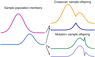
Figure 1: (Color Online) Illustration for the genetic operations of crossover and mutation. The shown curves represent imaginary parts of candidates for $G(\omega)$.

Now the principles of selection have to be discussed. Some of the best members of a generation are preserved without replacing them by their offspring. Furthermore, the trial Greens functions that are actually included into the new generation are obtained by entering the result of the GA operations into Eqs. (14) or (22) and calculating one iterative step. While in principle, pure GA operations could be used to find an optimal solution, the strict requirements imposed on a selfconsistent solution are more easily met by alternation of GA operations and iterative steps. As the new generation has more than twice as many members as the previous one, many are dropped according to their fitness values. In order to avoid premature convergence of the population to a suboptimal solution, some members with unfavorable fitness values are kept in the population, and some new random trial Greens functions are added to the population. The end of the evolution is determined, as in the iterative solution of the integral equations, by a member of the population reaching the target accuracy. We usually use fitness function values of $10^{-3}$ as a criterion for terminating the GA procedure. An additional advantage of the GA approach is the ease with which it can handle arbitrary kinds of constraints; they can be included as weighted components of the fitness function.

IV Results and discussions

First, we investigated band-width control Mott metal-insulator transition in the Hubbard model. The densities of states (DOS) at four different values of $U$ are shown in Fig. 2. As expected, quasi-particle peak as well as the upper and lower Hubbard bands are present in the metallic phase and transfer of spectral weight from quasi-particle peak to the Hubbard bands is clearly evident by reduction of the width of the central peak. In the insulating state, the central peak suddenly vanishes and a gap appears between upper and lower Hubbard bands. Further increasing $U$ leads to an increasing gap amplitude. The critical value of $U$ for Mott transition obtained from our impurity solver is $U_{c}\approx 2.5$. Compared to the critical value from numerical renormalization group method where $U_{c}\approx 2.94$ Bulla2 , our result underestimates the critical value of U due to the decoupling scheme. We note that in the metallic region, the height of our obtained DOS at the Fermi level is not fixed. This is due to the fact that two peaks in the imaginary part of the self-energy are quite close to the Fermi level, resulting in a numerical difficulty in getting a vanishing value of the imaginary part of the self-energy at Fermi level.

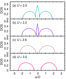
Figure 2: (Color Online) DOS calculated with GA method for particle-hole symmetric Hubbard model on Bethe lattice

Then, let us study the filling controlled Mott metal-insulator transition on the Hubbard model. In Fig. 3, we present the DOS as a function of doping at two different values of $U$. It is found that filling controlled metal-insulator transition occurs at $U=3$ while the system remains in metallic state at $U=2$. At $U=3$, we also investigate the effective mass

$$\frac{m^{\ast}}{m}=1-\frac{\partial{\rm Re}\Sigma(\omega)}{\partial\omega}\Big{|}_{\omega\rightarrow 0}$$ (33)

as a function of doping concentration. It is shown in Fig. 4 that the effective mass clearly displays a divergent behavior as doping concentration goes to zero which seems to obey Brinkman-Rice picture for the Fermi liquid Brinkman70 . In the small doping region, the carriers are more easily localized. We also studied the low frequency behavior near the Fermi level for the metallic state at different temperatures, as shown in Fig. 5. We obtained that the imaginary part of the self-energy does not exactly follow Fermi liquid behavior under the present decoupling scheme. However, as the temperature approaches zero, the negative imaginary part of the self-energy decreases. The precision of the results at very low temperature is presently limited numerically. Therefore, the exact behavior of the imaginary part of the self-energy at the Fermi level at zero temperature is beyond our reach. Even though our decoupling scheme qualitatively shows an acceptable behavior, from principal considerations exact Fermi liquid behavior is not to be expected from a decoupling approach.

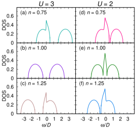
Figure 3: (Color Online) DOS for the asymmetrical Hubbard model on the Bethe lattice: filling controlled metal insulator transition.

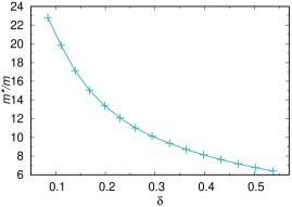
Figure 4: (Color Online) Effective mass at different fillings for the Hubbard model on the Bethe lattice.

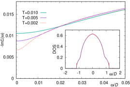
Figure 5: (Color Online) Self-energy at low temperature close to the Fermi level for the metallic state ($U=1$) for the particle-hole symmetric Hubbard model on the Bethe lattice. The inset shows the corresponding DOS.

We have also studied the Hubbard model with different types of bath as shown in Fig. 6. The influence of the bath has often been considered to be small since the self-consistent solution will not depend much on the initial guess of the bath. Our result shows that both Bethe lattice and hypercubic lattice produce qualitatively similar results for the Mott transition. However, our results show that different baths yield different critical interactions strengths $U_{c}$ at which the Mott transition sets in. For the Bethe lattice, we find $U_{c}^{\rm Bethe}\approx 2.5$, while for the hypercubic lattice, the result is $U_{c}^{\rm hypercubic}\approx 2.4$.

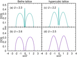
Figure 6: (Color Online) Comparison of Hubbard model with different kinds of bath: (left) Semicircle bath on Bethe lattice (right) Gaussian bath on hypercubic lattice. top two figures are metallic state, bottom two figures are insulator state just away from transition point

We now turn to a comparison of the two methods of solution we employed, the iterative method with Lorentzian broadening and the combined genetic algorithm and iterative method. The comparison of the CPU time needed for a selfconsistent solution is clearly in favor of GA: While in general the solution with pure iteration takes four times longer, near the Mott transition the iterative solution becomes very slow and inefficient. In Fig. 7, we show the results obtained with both methods for the same parameter values. In Fig. 7, top left, we can see that in the DOS there is a nonzero continuous connection between two Hubbard bands in the result obtained with Lorentzian broadening, which makes it difficult to distinguish the Mott transition clearly when $U$ approaches the critical value for the transition $U_{c}$ because the quasiparticle peak is very small in that case. Moreover, the Kondo peak will be greatly influenced by the amount of broadening. Different broadening will give different critical value of $U_{c}$. However, the combined GA and iteration method can give more precise results near the critical point which can be seen from the bottom left DOS figure. For the combined GA method, at $U=2.6$ we find an insulating state, while the Lorentzian broadening method still gives a metallic state at Fermi surface. This is due to the fact that the divergent behavior of the imaginary part of the self-energy just above the Mott transition cannot be correctly captured if there exists a finite broadening factor. However, in the GA method, the broadening factor can be even set to zero, which eliminates the numerical problem induced by the factor. The right panels of Fig. 7 shows the comparison of the imaginary part of the self-energy. It is found that GA method really gives a correct divergent behavior even close to the Mott transition at the Fermi level, while the Lorentzian broadening method does less well.

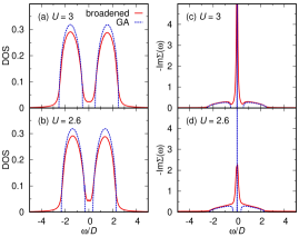
Figure 7: (Color Online) Comparison between the GA method and the iterative method with Lorentzian broadening for the particle-hole symmetric Hubbard model on the Bethe lattice: (top) DOS and self-energy for the insulating state with $U=3$. (bottom) DOS and self-energy close to the Mott transition with $U=2.6$.

We have also studied the Hubbard model with arbitrary degeneracy $N$. We have found that the decoupling scheme works nicely for $N=2$, but for $N>2$ there are some deviations from particle hole symmetry at half filling. We observe that the band positions and occupation numbers are correct, but some broadening of the upper Hubbard band is missing. This shows that the presently used decoupling of the three-particle Greens functions misses some terms that would contribute to the damping of the upper Hubbard band. We remedy this small deficiency by adding the ansatz $S(N)=-c(N-2)\Delta(\omega)$ in the denominator of $A$ (see Eq. 15) because this denominator is mainly responsible for the upper Hubbard band, and neglected contributions from higher order Greens functions should contribute an unknown function of $\Delta(\omega)$. The factor $c=0.5$ is found numerically from the requirement of particle hole symmetry at half filling, and the correction acts only for $N>2$ as $S(2)\equiv 0$. We get the results shown in Fig. 8, where we have calculated the spectral functions for various degeneracies $N$ at a temperature $T=0.01$. With increasing $N$, the total on-site Coulomb interaction increases so that the two Hubbard bands shift further away from the Fermi level. But the critical $U_{c}$ also increases with $N$. Therefore, at the same $U$, the system shows more metallicity for larger $N$, and transfer of spectral weight is observed from upper and lower Hubbard bands to the Kondo peak with increasing $N$. This result is consistent with the QMC result of Ref. Han98, .

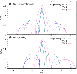
Figure 8: DOS for the finite $U$ Hubbard model for several values of the spin-orbital degeneracy $N$. The interaction strength is $U=2$, the hybridization strength $V=0.25$. (a) half-filling, (b) fixed impurity position $\varepsilon_{f}$.

For comparison, we have calculated the Periodic Anderson model with our code in Fig. 9. We observe a similar behavior of the spectral weight transfer as in the large $N$ Hubbard model. Meanwhile, Fig. 9 differs from the behavior shown in Ref. qi08, .

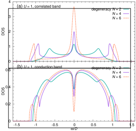
Figure 9: (Color Online) DOS for the periodic Anderson model for different values of the spin-orbital degeneracy $N$. (a) correlated band, (b) conduction band.

V Conclusions

We have presented the derivation and implementation of a solution of the single impurity Anderson model based on equations of motion and truncation. We employ a combination of genetic algorithms and iteration to solve the resulting integral equations. We demonstrate that our method is useful as an impurity solver in the context of dynamical mean field theory. We show results for the Mott metal insulator transition as a function of interaction strength $U$ and as a function of filling $n$, and also show the trend of weight transfer at different values of the spin-orbital degeneracy $N$.

We gratefully acknowledge support of the DFG through the Emmy Noether program.

References

- (1) A. Georges, G. Kotliar, W. Krauth, M. J. Rozenberg, Rev. Mod. Phys. 68, 13 (1996).
- (2) W. Metzner and D. Vollhardt, Phys. Rev. Lett. 62, 324 (1989).
- (3) A. Georges, G. Kotliar, Phys. Rev. B 45, 6479 (1992).
- (4) X. Y. Zhang, M. J. Rozenberg, G. Kotliar, Phys. Rev. Lett. 70, 1666 (1993)
- (5) H. Kajueter, G. Kotliar, Phys. Rev. Lett. 77, 131 (1996).
- (6) T. Fujiwara, S. Yamamoto, Y. Ishii, J. Phys. Soc. Jpn. 72, 777 (2003)
- (7) H. Keiter, J. C. Kimball, J. Appl. Phys. 42, 1460 (1971).
- (8) N. Grewe, H. Keiter, Phys. Rev. B 24, 4420 (1981).
- (9) Y. Kuramoto, Z. Phys. B 53, 37 (1983).
- (10) K. Haule, S. Kirchner, J. Kroha, and P. Wölfle Phys. Rev. B 64, 155111 (2001).
- (11) H. O. Jeschke, G. Kotliar, Phys. Rev. B 71, 085103 (2005).
- (12) J.-X. Zhu, R. C. Albers, J. M. Wills, arXiv:cond-mat/0409215v1 (unpublished).
- (13) Y. Qi, J. X. Zhu, C. S. Ting, Phys. Rev. B, in press, arXiv:0810.1738v1.
- (14) S. Onoda, M. Imada, J. Phys. Soc. Jpn. 70, 632 (2001), and J. Phys. Soc. Jpn. 70, 3398 (2001).
- (15) J. Hubbard, Proc. Roy. Soc. (London) A 276, 238 (1963).
- (16) L. Chioncel, L. Vitos, I. A. Abrikosov, J. Kollár, M. I. Katsnelson, and A. I. Lichtenstein, Phys. Rev. B 67, 235106 (2003).
- (17) V. Drchal, V. Janis, J. Kudrnovsky, V. S. Oudovenko, X. Dai, K. Haule and G. Kotliar, J. Phys.: Condens. Matter 17, 61 (2005).
- (18) J. E. Hirsch, R. M. Fye, Phys. Rev. Lett. 56, 2521 (1986).
- (19) M. Jarrell, Phys. Rev. Lett. 69, 168 (1992).
- (20) A. Georges, W. Krauth, Phys. Rev. Lett. 69, 1240 (1992).
- (21) M. J. Rozenberg, X. Y. Zhang, and G. Kotliar, Phys. Rev. Lett. 69, 1236 (1992).
- (22) P. Werner, A. Comanac, L. de’ Medici, M. Troyer, A. J. Millis, Phys. Rev. Lett. 97, 076405 (2006).
- (23) A. N. Rubtsov, V. V. Savkin, A. I. Lichtenstein, Phys. Rev. B 72, 035122 (2005).
- (24) M. Caffarel, W. Krauth, Phys. Rev. Lett. 72, 1545 (1994).
- (25) Q. Si, M. J. Rozenberg, G. Kotliar, A. E. Ruckenstein, Phys. Rev. Lett. 72, 2761 (1994).
- (26) R. Bulla, A. C. Hewson, and Th. Pruschke, J. Phys.: Condens. Matter 10, 8365 (1998).
- (27) R. Bulla, Phys. Rev. Lett. 83, 136 (1999).
- (28) D. J. Garcia, K. Hallberg, M. J. Rozenberg, Phys. Rev. Lett. 93, 246403 (2004).
- (29) M. Karski, C. Raas, G. S. Uhrig, Phys. Rev. B 77, 075116 (2008).
- (30) K. Held and D. Vollhardt, Eur. Phys. J. B 5, 473 (1998).
- (31) G. Kotliar, S. Y. Savrasov, K. Haule, V. S. Oudovenko, O. Parcollet, and C. A. Marianetti, Rev. Mod. Phys. 78, 000865 (2006).
- (32) D. N. Zubarev, Sov. Phys. Usp. 3, 320 (1960).
- (33) C. Lacroix, J. Phys. F: Metal Phys. 11, 2389 (1981).
- (34) C. Lacroix, J. Appl. Phys. 53, 2131 (1982).
- (35) G. Czycholl, Phys. Rev. B 31, 2867 (1985).
- (36) S. J. Wang, W. Zuo, W. Cassing, Nucl. Phys. A 573, 245 (1994).
- (37) H. G. Luo, Z. J. Ying, S. J. Wang, Phys. Rev. B 59, 9710 (1999).
- (38) G. P. Srivastava, J. Phys. A: Math. Gen. 17, L317 (1984).
- (39) E. D. Goldberg, Genetic Algorithms in Search, Optimization and Machine Learning, Kluwer Academic Publishers, Boston, 1989.
- (40) L. Rutkowski, Computational intelligence: methods and techniques, Springer, 2008.
- (41) M. Gen, R. W. Cheng, L. Lin, Networks models and optimization: multiobjective genetic algorithm approach, Springer-Verlag, London, 2008.
- (42) I. Grigorenko, M. E. Garcia, Physica A 284, 131 (2000).
- (43) I. Grigorenko, M. E. Garcia, Physica A 291, 439 (2001).
- (44) W. F. Brinkman, T. M. Rice, Phys. Rev. B 2, 4302 (1970).
- (45) J. E. Han, M. Jarrell, D. L. Cox, Phys. Rev. B 58, R4199 (1998).