Mg and TiO spectral features at the near-IR: Spectrophotometric index definitions and empirical calibrations

Abstract

Using the near-infrared spectral stellar library of Cenarro et al. (2001a,b), the behaviours of the Mg i line at 8807 Å and nearby TiO bands are analyzed in terms of the effective temperature, surface gravity, and metallicity of the library stars. New spectroscopic indices for both spectral features —namely MgI and sTiO— are defined, and their sensitivities to different signal-to-noise ratios, spectral resolutions, flux calibrations, and sky emission line residuals are characterized. The new two indices exhibit interesting properties. In particular, MgI reveals as a good indicator of the Mg abundance, whereas sTiO is a powerful dwarf-to-giant discriminator for cold spectral types. Empirical fitting polynomials that reproduce the strength of the new indices as a function of the stellar atmospheric parameters are computed, and a fortran routine with the fitting functions predictions is made available. A thorough study of several error sources, non-solar [Mg/Fe] ratios, and their influence on the fitting function residuals is also presented. From this analysis, a [Mg/Fe] underabundance of $\sim-0.04$ is derived for the Galactic open cluster M67.

1 Introduction

A powerful approach to unravel the stellar content of unresolved stellar systems is to interpret the integrated strengths of key spectral features on the basis of evolutionary stellar population synthesis models (e.g. Worthey 1994; Vazdekis et al. 1996; Vazdekis 1999; Vazdekis et al. 2003, hereafter VAZ03; Thomas, Maraston & Bender 2003; Bruzual & Charlot 2003; Maraston 2005; Schiavon 2007). These models make use of theoretical isochrones and spectral stellar libraries to predict integrated line-strengths and/or spectral energy distributions (SEDs) corresponding to simple stellar populations (SSPs) of a given age, overall metallicity, abundance pattern, initial mass function, and star formation history.

Up to date, major progress in this kind of studies has been achieved in the optical spectral range. The Lick/IDS stellar library (Gorgas et al. 1993; Worthey et al. 1994) has constituted so far the reference system for most optical work on this topic. However, thanks to the developing of much improved optical stellar libraries that superseed the capabilities of the Lick/IDS library, like e.g. Jones (1998), ELODIE (Prugniel & Soubiran 2001, 2004; Prugniel et al. 2007), STELIB (Le Borgne et al. 2003), the Indo-US stellar library (Valdés et al. 2004), and MILES (Sánchez-Blázquez et al. 2006; Cenarro et al. 2007), a new generation of SSP models in the optical region (e.g. Vazdekis 1999; Bruzual & Charlot 2003; PÉGASE-HR, by Le Borgne et al. 2004; Vazdekis et al. 2009, in preparation) is now available. The larger spectral coverage and better spectral resolution of the new models have motivated the development of new analysis approaches that, rather than focusing on single spectral features, are based on fitting techniques over the full spectrum that are potentially useful for reconstructing in first order the star formation histories of galaxies (e.g. Panter et al. 2003; Cid Fernandes et al. 2005; Mathis, Charlot, & Brinchmann 2006; Ocvirk et al 2006a,b; Panter, Heavens, & Jimenez 2007; Koleva et al. 2008).

Aside from the above work, there exists an important effort to advance in our understanding of complementary spectral regions which are governed by different types of stars, like the ultraviolet (e.g. Fanelli et al 1992; Gregg et al. 2004; Heap & Lindler 2007) and the infrared (e.g. Ivanov et al. 2004; Ranade et al. 2004, 2007a,b; Mármol-Queraltó et al. 2008). In particular, aimed at providing reliable SSP model predictions for the near-infrared (near-IR) spectral region around Ca ii triplet at $\sim 8600$ Å, an extensive spectral stellar library at $\lambda\lambda~{}8348-9020$ Å (FWHM$=1.5$ Å) that comprises 706 stars over a wide range of atmospheric parameters was developed by Cenarro et al. (2001a; hereafter CEN01a). Subsequent libraries like STELIB and the Indo-US also include the Ca ii triplet region. Initially, the library in Cenarro et al. (2001) was particularly devoted to understand the behaviour of the Ca ii triplet in individual stars. With this aim, improved line-strength indices for this spectral feature (namely CaT, PaT, CaT^∗) which are especially suited to be measured in the integrated spectra of stellar populations were defined (CEN01a). Also, to minimize uncertainties and systematic errors of the empirical calibration of the indices, a homogeneous system of revised atmospheric parameters for the library stars was derived in Cenarro et al. 2001b (hereafter CEN01b). Puting all these ingredients together, the behaviour of the Ca ii indices as a function of the stellar atmospheric parameters was computed by means of so-called empirical fitting functions (Cenarro et al. 2002; hereafter CEN02), which were implemented into the evolutionary synthesis code of VAZ03 to predict the integrated indices and the near-IR SEDs for SSPs of different ages, metallicities, and IMFs.

The present paper can be considered as an extension of the above project to two nearby spectral features: the Mg i line at $\lambda$ 8807 Å and the molecular bands of TiO at $\lambda\lambda$ 8432, 8442, 8452 Å and $\lambda\lambda$ 8860, 8868 Å. As it was already shown in Cenarro et al. (2003) for a sample or 35 early-type galaxies, both spectral features —together with the Ca ii triplet— can play an important role to characterize the properties of old and intermediate-aged stellar populations. The fact that Mg is overabundant with respect to Fe in massive elliptical galaxies and tightly correlates with the velocity dispersion (e.g. Dressler et al. 1987; Worthey et al. 1992; and others) turns Mg indices into a key element to constrain galaxy star-formation and evolution theories. Also, it is worth stressing the importance of calibrating several spectroscopic indicators in a relatively narrow spectral region, as in contrast with stellar population studies in which blue and red indicators are employed together, the ages and metallicities derived from a set of nearby indices are expected to be consistent even for composite stellar populations.

Therefore, the main objective of this paper is to carry out a comprehensive study of the Mg i and TiO features in individual stars, so that their dependences with the atmospheric parameters are calibrated and quantyfied via empirical fitting functions. A forthcoming paper by Vazdekis et al. (in preparation) will be devoted to present and discuss the corresponding SSP model predictions (both based on such fitting functions and from the SEDs in Vazdekis et al. 2003) in comparison with galactic observational data.

Section 2 is focused on the definition of new line-strength indices for the Mg i line and the TiO bands and on the comparison with those of previous work. The new index sensitivities to different spectral resolutions, signal-to-noise ratios, flux calibration, reddening uncertainties, and residuals of sky lines and telluric absorptions are analyzed. Also, accurate formulae for estimating random errors in the new index measurements are provided. After a qualitative description of the Mg i line and the TiO bands strengths on the basis of the library stars, Section 3 is devoted to the mathematical fitting procedure of the index strengths as functions of the stellar atmospheric parameters, providing the significant terms, coefficients, and statistics of the derived fitting functions. A thorough analysis of the fitting function residuals and possible error sources is herein presented, accounting for the uncertainties in the input atmospheric parameters, the flux calibration, and the effect of different [Mg/Fe] ratios in the Mg i line fitting functions. A qualitative comparison with MgI and sTiO predictions based on theoretical work is presented in Section 4. To conclude, Section 5 is reserved to discuss and summarize the main contents and results of this paper.

2 MgI and TiO spectroscopic indices

Figure 1: Spectra of the stars HD 186568 (B8 III), HD 89025 (F0 III), HD 216228 (K0 III) and HD 114961 (M7 III) in the spectral range of the stellar library from CEN01a. The strongest features in this region are marked: the Paschen Series (from P11 to P20), the Ca ii triplet (Ca1, Ca2 and Ca3), several metal lines and telluric absorptions. The Mg i line and the molecular bands of TiO and VO are indicated in spectra (c) and (d) respectively.

Before focussing on the definition of new line-strength indices for the measurement of the Mg i and TiO spectral features, it is worth making a brief description of the spectral range under study. The existence of other absorption lines around the spectral features of interest is indeed decisive for a proper location of the index bandpasses. As in CEN01a, the strongest spectral features around 8600 Å are labelled in Figure 1 for a subsample of representative spectral types; the MgI line and TiO bands concerning this paper are indicated in spectra (c) and (d) respectively. It is readily seen from that figure that the H Paschen series completely dominates the spectra of the hottest stars. Its strength decreases with the decrasing temperature at the time that several metal lines become stronger. For G, K and early-M spectral types, the spectra are mainly governed by the Ca ii triplet, the Mg i line and many other Fe and Ti absorption lines. Finally, intermediate and late-M types exhibit strong molecular bands of TiO and VO which modulate the shape of the local continuum. See CEN01a and CEN02 for a more detailed description of the above behaviours.

2.1 Previous index definitions

Despite most previous papers dealing with the present spectral range were mainly focussed on the Ca ii triplet, a few of them already considered the Mg i line at 8807 Å and the TiO bands at $\lambda\lambda$ 8432, 8442, 8452 Å and $\lambda\lambda$ 8860, 8868 Å. This was the case of Díaz, Terlevich & Terlevich (1989, hereafter DTT) and Carter, Visvanathan & Pickles (1986, hereafter CVP), who provided index definitions for the Mg i line and the TiO bands respectively. Table 1 lists the bandpass limits of the corresponding indices as defined in the above papers. In turn, Figures 2 and 3 illustrate the suitability of these indices when measured over different spectral types.

Table 1: Definition of previous and new indices for the near-IR Mg i line ($\lambda$ 8807 Å) and TiO bands ($\lambda\lambda$ 8432, 8442, 8452 Å; $\lambda\lambda$ 8860, 8868 Å). Codes for the references are as follow: CVP (Carter, Visvanathan & Pickles 1986), DTT (Díaz, Terlevich & Terlevich 1989), TW (This work). Types $c$–$a$, $c$–$m$, $g$–$a$ and $g$–$s$ refer to classical–atomic, classical–molecular, generic–atomic and generic–slope–like indices respectively.

Index	Type	Central	Continuum
		Bandpass (Å)	Bandpasses (Å)
MgI (DTT)	$c$–$a$	8799.5–8814.5	8775.0–8787.0
			8845.0–8855.0
MgI (TW)	$g$–$a$	8802.5–8811.0	8781.0–8789.0
			8831.0–8835.5
			8841.5–8846.0
TiO1 (CVP)	$c$–$m$	8450.0–8700.0	8350.0–8400.0
			8750.0–8800.0
TiO2 (CVP)	$c$–$m$	8890.0–9060.0	8790.0–8840.0
			9100.0–9150.0
sTiO (TW)	$g$–$s$	none	8474.0–8484.0
			8563.0–8577.0
			8619.0–8642.0
			8700.0–8725.0
			8776.0–8792.0

In the 90s, the indices defined by DTT were the most widely employed to measure the strengths of the Ca ii triplet and the Mg i lines. For the Mg i spectral feature they defined a classical atomic index that consists of a central bandpass enclosing the Mg i line, and two continuum bandpasses located at both sides —blue and red— of the central one. In spite of being a well-defined index for F$-$K spectral types, it suffers from two main limitations: i) the presence of strong Paschen lines (P11 and P12) in early spectral types makes the derived pseudo-continuum to be unreliable (Figure 2a), and ii) the proximity of the red continuum bandpass to the TiO break around 8600 Å makes the index to be very sensitive to spectral resolution and velocity dispersion broadening (Figure 2c). This is particularly critical for the integrated spectra of galaxies in which TiO bands may be prominent (see e.g. the SEDs predicted in VAZ03), and typical velocity dispersions are above $\sim 100~{}{\rm kms}^{-1}$. In any case, it is fair noting the intrinsic difficulty of defining a Mg i line-strength index in a spectral region dominated by strong absorption lines. This is particularly evident in the case of the earliest spectral types (see Figure 2a), for which the Mg i line is wery weak and the wings of the Paschen lines are blended thus decreasing the true continuum level.

The work by CVP defined classical molecular indices to measure the strength of the TiO bands. Again, the index consists of two continuum bandpasses and a very wide central bandpass for the TiO break at $\sim 8450$ Å (see Table 1). Because of the width of the central bandpass, the index turns out to be sensitive the Ca ii triplet and the Paschen lines for those spectral types in which the above features dominate the spectrum (Figures 3a,b). Such a Ca and H contamination for most spectral types is obviously not desired when trying to understand the behaviour of the TiO bands with the stellar atmospheric parameters, as it would translate into a blurring of age and metallicity effects if the TiO index were used as a tool for stellar population diagnostics.

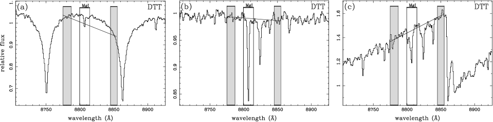
Figure 2: Index definition by DTT for the Mg i line over different spectral types. The spectra, taken from the stellar library of CEN01a, correspond to HD161817 (A2 VI; $a$), HD25329 (K1 Vsb; $b$) and HD148783 (M6 III; $c$). Grey and open bands illustrate, respectively, the location of continuum and central bandpasses (see Table 1). Solid lines represent the local pseudo-continua computed by means of error weighted least-squares fits to all the pixels in the continuum bandpasses.

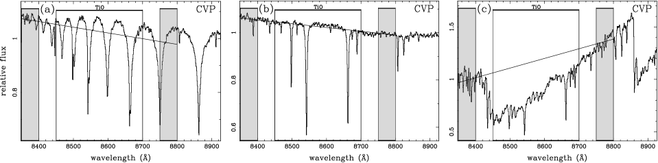
Figure 3: Index definition for the TiO bands by CVP (TiO₁; see Table 1) over different spectral types. Spectra, bandpasses color code, and solid lines are the same as in Fig. 2.

2.2 New index definitions

In CEN01a we introduced new type of line-strength indices, namely generic indices, which allow the definition of an arbitrary but precise number of continuum bandpasses to derive the pseudo-continuum level. It is computed as an error-weighted, least-squares linear fit to all the pixels of these continuum bandpasses. Generic indices also allow the inclusion of various bandpasses for adjacent spectral features, which are thus measured simultaneously -using different relative weights- under the same pseudo-continuum. As we report in that paper, the above improvements are highly advantageous in regions densely populated by other spectral features, telluric lines or strong sky emission lines, as it is the case for the near-IR spectral range. CaT, PaT and CaT^∗ are examples of generic indices for the Ca ii triplet and three lines of the H Paschen series (see details in CEN01a).

The new generic indices that we characterize here, MgI and sTiO, were formerly measured in Cenarro et al. (2003) for a sample of early-type galaxies. We devote the current paper to provide full details on their definition, sensitivities, and behaviour with the stellar atmospheric parameters.

2.2.1 The MgI index

The MgI index has been defined as a generic index consisting of three continuum bandpasses and one spectral-feature bandpass for the Mg i line. Figure 4 illustrates the Mg i index defined in this work when measured over the same spectra as in Fig. 2, and the bandpasses limits are listed in Table 1. The location and width of these bandpasses were established in order to derive a reliable pseudo-continuum for all the spectral types even when the spectra are broadened up to 300 ${\rm kms}^{-1}$. Also, since we are interested in measuring MgI on broadened galaxy spectra, we ensured that the TiO break at $\lambda$ 8860 Å was not affecting the pseudo-continuum level. Note however that, because of the problem reported in the previous section, the pseudo-continuum derived for early spectral types is still slightly below the true level (Fig. 4a). With the aim of defining a reliable indicator of Mg abundance, we tried to avoid as much as possible the presence of other metal lines within the spectral-feature band (e.g. see Fig. 4c). This is why we preferred to define a quite narrow characteristic bandpass, even though it increases the sensitivity of the index to the spectral resolution. A reasonable compromise between both requirements was finally established.

2.2.2 The sTiO index

For the measurement of the TiO bands we introduce a new type of generic index which will be referred to as slope index. Slope indices are defined as the ratio between the pseudo-continuum values at the central wavelengths of any two continuum bandpasses. In this sense, they can be considered as a measurement of the local pseudo-continuum slope. It is important to note that, although slope indices just consider the pseudo-continuum values at the center of two continuum bandpasses, the total number of continuum bandpasses driving the pseudo-continuum level can be as large as desired. In practice one actually performs an error-weighted least-squares linear fit to all the pixels within the full set of considered continuum bandpasses. After that, the linear fit is evaluated at the central wavelengths of the first and last of those bandpasses.

This new concept of index was conceived with the aim of measuring the slope of the continuum around the Ca ii triplet, mainly governed by molecular absorptions (TiO and VO) in mid and late-M spectral types. Given that the location of the five continuum bandpasses for the indices CaT, PaT or CaT^∗ leads to a reliable pseudo-continuum for all the spectral types, we took advantage of the previous indices to define the slope index sTiO. In particular, it is defined as the ratio between the pseudo-continuum values, $C(\lambda)$, at the central wavelengths of the reddest and bluest continuum bandpasses (see Table 1), that is,

$${\rm sTiO}=\frac{C(\lambda 8784.0)}{C(\lambda 8479.0)}.$$ (1)

At variance with other spectrophotometric indices, sTiO is potentially sensitive to flux calibration uncertainties (hence extinction effects) given that its continuum bandpasses spread over more than 300 Å. On the other hand, it is particularly unsensitive to low signal-to-noise ratios as the slope gets robustly constrained by 5 bandpasses that overall cover 88 Å. These and other effects will be discussed in Section 2.4.

2.2.3 MgI and sTiO measurements for the library stars

The new indices have been measured for all the spectra in CEN01a at the nominal resolution of the library, that is, FWHM$=1.5$ Å or $\sigma=22.2$ km s^-1. Table 10 lists the index measurements and their errors, which account for the photon noise and radial velocity uncertainties, the later including typical errors in wavelength calibration. This database is also available at
http://www.ucm.es/info/Astrof/ellipt/MgIsTiO.html

The actual measurements have been performed with indexf (Cardiel 2007), a C++ program specially written to compute atomic, molecular, break, generic-atomic, generic-break and slope indices in wavelength-calibrated FITS spectra. This program is available at
http://www.ucm.es/info/Astrof/software/indexf

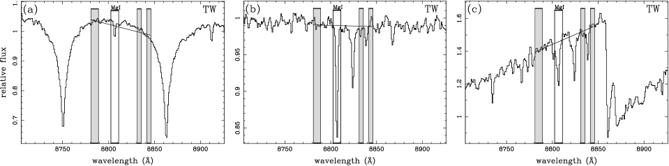
Figure 4: New index definition (this work; TW) for the Mg i line, MgI, over the same spectral types of Fig. 2. Again, grey and open bandpasses illustrate, respectively, the location of continuum and central bandpasses (see Table 1), whilst solid lines represent the local pseudo-continua derived from error weighted least-squares fits to all the pixels in the continuum bandpasses.

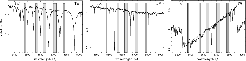
Figure 5: New index definition (this work; TW) for the TiO bands, sTiO, over the same spectral types of Fig. 2. The five continuum bandpasses are those corresponding to the CaT indices in CEN01a. The two bandpasses that define the sTiO value (see Eq. 1) are illustrated in dark grey.

2.3 Conversions between the new and previous index systems

Table 2: Calibrations between different index systems. $\sigma_{\rm r.m.s}$: unbiased standard deviation of the fit. N: Number of stars in the fit. T_eff (K): Effective temperature region where the calibration was obtained. These calibrations are graphically displayed in Fig. 6.

Calibrations	$\sigma_{\rm r.m.s}$	$N$	Teff (K)
MgI = 0.119 + 0.864 MgI(DTT)	0.07	560	2750–6300
sTiO = 0.822 + 3.397 TiO1(CVP)	0.07	29	2750–3700
MgI(DTT) = MgI(DTT)DTT	0.16	100	3425–6800

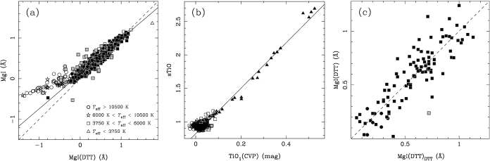
Figure 6: Comparison between the different systems of indices. Diagrams (a) and (b) compare the new indices MgI and sTiO with the corresponding MgI (by DTT) and TiO₁ (by CVP), both measured in this work over the 706 stars of our stellar library (CEN01a). Diagram (c) shows the MgI by DTT measured in our and their spectra (MgI(DTT) and MgI(DTT)_DTT respectively) for the subsample of stars in common. Symbol types, indicating different ranges of effective temperature, are given in panel (a). The dashed line in panels (a) and (c) shows the one-to-one relation. Grey symbols are stars deviating more than $3\sigma$ from the fitted relation, whereas open symbols refer to those stars with effective temperatures outside the fitted range. The solid line marks the most significant fit to the symbols in black (see Table 2).

For those readers interested in transforming old system data of indices into the new ones (or vice-versa), this section provides a set of calibrations to make conversions from one system to the other. Table 2 lists the derived relations and Figure 6 illustrates the corresponding fits.

Using the 706 library stars from CEN01a, we have compared the measurements of the indices MgI(DTT) and TiO₁(CVP) with the ones corresponding to the new MgI and sTiO. The calibrations were computed by means of error weighted least-squares fits to a straight line that, in both cases, turned out to be statistically significant. The location and width of the MgI(DTT) bandpasses (see Section 2.1) causes hot stars to depart from the general trend of the rest of the library stars. In order to ensure the quality of the fit, we have restricted the range of the calibration excluding from the fit those stars with high temperatures (Fig. 6a). The calibration between the TiO indices (Fig. 6b) was derived just considering those stars cold enough to exhibit molecular bands in their spectra. Otherwise the fit would be strongly dominated by the behaviour of earlier spectral types for which the indices do not measure TiO. In all fits, stars within the valid range of $T_{\rm eff}$ but deviating more than $3\sigma$ from the fitted relation were also rejected.

Finally, for a subsample of stars in common with the stellar library from DTT, we have compared the MgI(DTT) values given in DTT (MgI(DTT)_DTT) with the ones measured over our spectra. Note that, since the measured index is the same in both cases, systematic differences between the two sets of measurements could only arise from differences in their spectrophotometric systems. However, no significant differences have been found (Fig. 6c).

To conclude, it is important to remind the reader that the two first calibrations in Table 2 should only be applied once the spectra are on the same spectrophotometric system (that is, equally flux calibrated and at the same spectral resolution) as the stellar library of CEN01a. If that is not the case, a prior calibration like the last one in Table 2 should be applied before.

2.4 Sensitivities of the new indices to different effects

This section is devoted to characterize the sensitivity of the indices MgI and sTiO to the signal-to-noise ratio, the velocity dispersion broadening (or spectral resolution), relative flux calibration, extinction effects, and sky subtraction residuals.

2.4.1 Signal-to-noise ratio

In CEN01a, it was presented a thorough study on the computation of random errors —arising from photon noise— for generic indices. We refer the reader to the Appendix A2 of that paper for full details about the procedure (see also Cardiel et al. 1998). In those papers, it was demonstrated that it is possible to estimate the predicted random errors of atomic indices as a function of the signal-to-noise (S/N) ratio per angstrom —hereafter $S\!N(\rm\AA)$—, by means of analytical expressions of the form

$$\sigma[{\cal I}_{\rm a}]\simeq\displaystyle\frac{c_{1}-c_{2}\;{\cal I}_{\rm a}}{S\!N(\rm\AA)},$$ (2)

where [${\cal I}_{\rm a}$] refers to any atomic index (either classical or generic), and the coefficients $c_{1}$ and $c_{2}$ —which depend on the index definition— can be computed analytically for classical indices, and empirically for generic ones (see Appendix 3 in CEN01a).

Figure 7: Empirical estimation of the constant factors $c_{1}$ and $c_{2}$ in Eqs. (3) and (4), for MgI and sTiO, respectively. The least-squares fits to straight lines have been performed rejecting data iteratively outside the 99.73 per cent confidence level.

Following the empirical approach for our generic indices, Figure 7 displays the product $S\!N(\rm\AA)\times\sigma[{\cal I}_{\rm a}]$ versus the index value for all the library stars in CEN01a. As expected for generic atomic indices, MgI exhibits a clear linear relationship, thus supporting previous results that Eq. 2 is indeed a good approach to the S/N dependence of random errors. Interestingly, although sTiO is not an atomic index, it is also found to follow a nice linear behaviour when included in Fig. 7, despite it exhibits an opposite trend (what is understandable as slope indices are conceptually different to atomic indices; see Section 2.2.2. Note also that sTiO has no units, so the labels of the axes are not strictly correct in this case). A least-squares fit to all data provides

$$\begin{array}[]{@{}r@{\;}c@{\;}l}\sigma[\rm MgI]&\simeq&\displaystyle\frac{3.552-0.3384\;\rm MgI}{S\!N(\rm\AA)},\\ \end{array}$$ (3)

and

$$\begin{array}[]{@{}r@{\;}c@{\;}l}\sigma[\rm sTiO]&\simeq&\displaystyle\frac{-0.08914+0.4366\;\rm sTiO}{S\!N(\rm\AA)}.\\ \end{array}$$ (4)

As expected, for MgI, $c_{1}$ is one order of magnitude larger than $c_{2}$, thus reinforcing the idea that photon noise errors in generic atomic indices are barely dependent on the index values. However, this is not the case for slope indices like sTiO. In fact, $c_{2}$ dominates the error dependence, in the sense that the larger the index, the larger the error.

Based on the above equations we estimate that, for the typical indices of an old, solar-metallicity SSP (VAZ03), it is required $S\!N(\rm\AA)\sim 50$ Å^-1 and $\sim 3$ Å^-1 to measure, respectively, MgI and sTiO with a 10 per cent uncertainty. It is therefore clear that, while sTiO is optimized to be measured on low signal-to-noise ratio spectra (a potential application for high redshift galaxies and extragalactic globular clusters is immediately derived), MgI demands relatively high quality spectra to drive reliable results. This is unavoidably the price one has to pay for defining MgI as a “pure” Mg indicator, with a very narrow central bandpass that prevents from the contamination with other nearby lines.

2.4.2 Spectral resolution

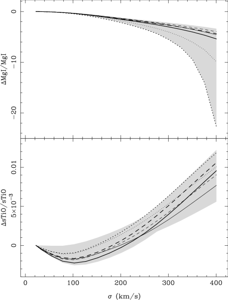
Figure 8: Broadening correction $\Delta$MgI/MgI and $\Delta$sTiO/sTiO as a function of total $\sigma$. Corrections have been computed by convolving model spectra by VAZ03 with Gaussians from $\sigma=25$ km s^-1 up to $\sigma=400$ km s^-1 in steps of 25 km s^-1. $\Delta I/I$ is zero for $\sigma=$22.2 km s^-1 (the spectral resolution of the stellar library in CEN01a). Different line types are employed to illustrate the broadening corrections for a set of representative models of different ages, metallicities, and IMFs: solid (12.6 Gyr, [M/H]$=0.0$), dotted (1.0 Gyr, [M/H]$=0.0$), and dashed (12.6 Gyr, [M/H]$=-0.7$), with thick and thin lines corresponding to IMF slopes of $\mu=1.3$ (Salpeter) and 2.8 respectively. The polynomial coefficients of such broadening corrections are given in Table 3. The grey area illustrates the region covered by the broadening corrections obtained for the whole set of SSP spectra of VAZ03.

With the aim of studying the sensitivity of MgI and sTiO to the spectral resolution or galaxy velocity dispersion broadening ($\sigma$), we broadened the whole set of SSP model spectra of VAZ03 by convolving with Gaussians of $\sigma$ varying from 25 up to $400$ km s^-1, in steps of 25 km s^-1. The indices were thus measured for the full set of broadened spectra and, for each model, we fitted a third-order polynomial to the relative changes of the index values as a function of velocity dispersion,

$${\frac{{\cal I}(\sigma)-{\cal I}(\sigma_{0})}{{\cal I}(\sigma)}=a+b\sigma+c\sigma^{2}+d\sigma^{3}\equiv p(\sigma)},$$ (5)

where $\sigma_{0}=22.2$ km s^-1 is the nominal resolution of the VAZ03 models (FWHM = 1.50 Å), and $\sigma$ is any generic resolution in the same units. Note that Eq. 5 is computed as a function of the overall spectral resolution, so that for $\sigma=\sigma_{0}$, $p(\sigma_{0})=0$.

Table 3 provides the derived coefficients for MgI and sTiO measured over a number of representative SSP models. Figure 8 illustrates the obtained $\Delta$MgI/MgI and $\Delta$sTiO/sTiO values for this set of representative models. The grey region represents the locus of broadening corrections for the whole SSP model spectral library.

It is worth noting that, thanks to the high stability of the continuum bandpasses, the index sTiO is formally insensitive to broadening, with largest corrections being only $\sim 1$ per cent at $\sigma\sim 400$ km s^-1. On the other hand, MgI turns out to be quite dependent on spectral resolution. This is due to the small width of the central bandpass —chosen this way to preserve as much as possible the Mg abundance sensitivity— and to the intrinsic weakness of the Mg i line (EW $<1$ Å). In fact, at $\sigma=300$ km s^-1, Mg i decreases by $\sim 78.2\pm 6.6$ per cent w.r.t. the value at $\sigma_{0}=22.2$ km s^-1, with uncertainties accounting for the different broadenings derived from the full set of SSPs. This effect decreases down to $\sim 56.8\pm 0.6$ per cent at $\sigma=200$ km s^-1, which can be considered as a reasonable limiting resolution to neglect broadening correction differences due to distinct SSP templates.

As it was already discussed in VAZ03 for the Ca ii triplet indices, the use of SSP model spectra to match the effects of galaxy broadening is a better approach than the use of single stellar spectra, as the later shows even large variations among different spectral types. In any case, the user should still keep in mind that systematic differences —arising, for instance, from different abundance ratios or local flux calibration mismatches— may exist between real galaxies and the best matched SSP models. For this reason, whenever it is feasible, an alternative approach is that of broadening the galaxy spectra and the SSP models up to the largest spectral resolution of the galaxy sample. The success of this approach for the MgI and sTiO indices of elliptical galaxies over a range in mass was illustrated in Cenarro et al. (2003).

Table 3: Coefficients of the broadening correction polynomials $\Delta{\cal I}/{\cal I}=a+b\sigma+c\sigma^{2}+d\sigma^{3}$ for MgI and sTiO, for a representative set of Vazdekis et al. (2003) SSP models of different IMF slopes $\mu$, metallicities [M/H], and ages. $\Delta{\cal I}/{\cal I}$ is zero for $\sigma=$22.2 km s^-1, the spectral resolution of the stellar library in CEN01a.

${\cal I}$	$\mu$	[M/H]	Age (Gyr)	$a(\times 10^{-3})$		$b(\times 10^{-5})$		$c(\times 10^{-7})$		$d(\times 10^{-9})$
sTiO	1.3	0.0	1.0	0.	909	$-4.$	782	3.	179	$-0.$	334
	1.3	0.0	12.6	1.	421	$-7.$	219	3.	764	$-0.$	368
	1.3	$-0.$7	12.6	0.	895	$-4.$	648	2.	828	$-0.$	262
	2.8	0.0	1.0	0.	753	$-3.$	941	2.	536	$-0.$	241
	2.8	0.0	12.6	1.	064	$-5.$	434	2.	947	$-0.$	296
	2.8	$-0.$7	12.6	1.	145	$-5.$	879	3.	333	$-0.$	341
MgI	1.3	0.0	1.0	1030.	686	$-5544.$	545	4297.	828	$-1061.$	284
	1.3	0.0	12.6	61.	862	$-207.$	795	$-259.$	635	$-4.$	898
	1.3	$-0$.7	12.6	44.	553	$-124.$	534	$-349.$	063	$27.$	095
	2.8	0.0	1.0	225.	317	$-1124.$	182	539.	861	$-215.$	236
	2.8	0.0	12.6	42.	790	$-127.$	770	$-295.$	117	$10.$	880
	2.8	$-0$.7	12.6	37.	606	$-95.$	207	$-340.$	763	$29.$	619

2.4.3 Flux calibration and reddening correction

There is not a simple recipe to quantify analytically the sensitivity of an index to the uncertainties in the relative flux calibration, as it does not only depend on the index definition itself, but also on the uncertainties of the response curves derived for a given observing run. In general, the sensitivity of any spectroscopic index to flux calibration gets larger as the spectral coverage of its sidebands increases. In this sense, it is clear that sTiO is particularly sensitive to systematics in the flux calibration and the reddening correction, as it basically measures the slope of the pseudo-continuum in a spectral window of $\sim 300$ Å. For instance, assuming the Galactic interstellar extinction of Fitzpatrick (1999), the effect of reddening in the sTiO index is given by

$$\frac{{\rm sTiO}_{\rm ext}-{\rm sTiO}_{0}}{{\rm sTiO}_{0}}=0.087\times E(B-V),$$ (6)

where sTiO_ext is the reddened index value (for a colour excess of $E(B-V)$ and R = 3.1) and sTiO₀ the extinction corrected one. This means that to ensure systematics in the sTiO index below $1\%$, reddening correction uncertainties should not be larger than $E(B-V)\sim 0.1$ mag. MgI, however, is basically stable under flux calibration variations and extinction corrections.

As it will be discussed in Section 3.3.2 with the aim of explaining the observed fitting function residuals, it is important to note that the main source of random errors for the sTiO index turns out to be the random uncertainties in the determination of the response curve. This stresses the importance of an accurate flux calibration and extinction correction before performing any meaningful comparison between evolutionary synthesis model predictions and measured spectra.

2.4.4 Sky emission lines and telluric absorptions

Sky emission lines —produced by the OH radical (e.g. Rousselot et al. 2000)— and telluric absorptions —due to water vapour and other molecules (e.g. Stevenson 1994, Chmielewski 2000)— are common features at the near-IR spectral range. A careful data reduction is necessary for a proper removal of these effects, although a detailed description of specific techniques is out of the scope of this paper. Rather than that, we just aim to compare qualitatively the potential sensitivities of our indices to the above contaminations. An absolute study is not possible at this point, as it would strongly depend on the quality of the final spectra.

Because of the narrow index definition and the intrinsic weakness of the Mg i line, MgI is quite more sensitive to sky line and telluric absorptions residuals than sTiO. In principle, since the sTiO slope is well constrained by five continuum bandpasses, a few deviating pixels in its continuum bandpasses would not alter the index value significantly (actually, generic indices are particularly insensitive to sky line residuals; Section 2.2). A different situation would be that in which a strong —not properly removed— telluric absorption is affecting the red —or blue— sides of the index definition. In this case, the local slope of the continuum would be fictitiously biased and the index would be highly unreliable. Fortunately, this is not the case for spectra at the local rest-frame (like the stellar library of CEN01a). In any case, it is worth noting that the strong telluric absorption at $\lambda\ga 8940$ Å may affect the MgI and sTiO indices of objects with radial velocities larger than $\sim 3200$ and $5000\,{\rm km~{}s}^{-1}$ respectively.

3 The dependence of the MgI line and TiO bands on the stellar atmospheric parameters

3.1 Qualitative behaviour

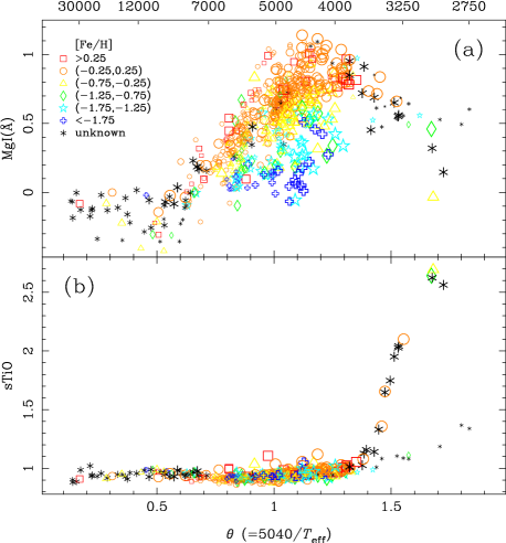
Figure 9: MgI and sTiO indices versus $\theta(\equiv 5040/T_{\rm eff})$ for the whole stellar library in CEN01a. Different symbols are used to indicate different ranges of metallicities (as in the key), while sizes are related with surface gravity, in the sense that the smaller the symbol (dwarfs), the higher the gravity. On the top, the effective temperature scale is given.

As a first step to understand the behaviour of the Mg i line and TiO bands as a function of the stellar atmospheric parameters, this section describes, from a qualitative point of view, the effects of effective temperature ($T_{\rm eff}$ or $\theta\equiv 5040/T_{\rm eff}$), surface gravity ($\log g$) and metallicity ([Fe/H]) on the strength of both spectral features. Figure 9 illustrates the MgI and sTiO indices versus $\theta$ for all the stars in CEN01a.

3.1.1 The stellar atmospheric parameters

The stellar atmospheric parameters employed throughout this work are those derived in CEN01b, where, after an exhaustive compilation from several hundreds of bibliographic sources, the different sources were calibrated and corrected onto the system established by Soubiran, Katz & Cayrel (1998) to end up with a homogeneous set of atmospheric parameters (see details in CEN01b). Although more recent determinations of $T_{\rm eff}$, $\log g$, and/or [Fe/H] have appeared since 2001 for some library stars, we preferred to keep the parameters quoted in CEN01b to preserve full consistency with the CaT, PaT, and CaT^∗ fitting functions given in CEN02, as well as with the corresponding SSP SEDs predicted in VAZ03. It is worth noting that, in Cenarro et al. (2007), an updated extension of the compiling work in CEN01b was carried out for MILES, which in turn includes 403 stars in common with CEN01a. Using all those stars in CEN01a for which any of the three atmospheric parameters in Cenarro et al. (2007) was updated with respect to CEN01b (194 stars in $T_{\rm eff}$, 133 in $\log g$, and 116 in [Fe/H]), we determined that the differences between the old and new final determinations are null on average, with r.m.s. standard deviations of $\sigma T_{\rm eff}\sim 72$ K, $\sigma\log g\sim 0.22$ dex, and $\sigma$[Fe/H]$\sim 0.1$ dex. Since there exist not statistically significant offsets between both datasets in any of the three atmospheric parameters that may lead to systematic effects, and the scatter of the distributions is smaller than the typical uncertainties in the atmospheric parameters (see Section 3.3.1), we are confident that using the parameters in CEN01b is not compromising at all the quality of the results that we present in this work.

3.1.2 The Mg i line

Figure 10: Metallicity and gravity effects on the strength of the Mg i line at 8807 Å for a subsample of stars from CEN01a. Panel (a) shows stars with similar temperature and gravity but spanning a wide range in metallicity. Panel (b) displays a sequence in gravity for stars with similar temperature, and metallicity around solar. Temperatures in K are given in brackets. All the spectra have been normalized and reproduced using the same scale. It is clear the increasing strength of the Mg i line with the increasing [Fe/H]. The effect of $\log g$ in the strength of the Mg i line is very mild, with intermediate $\log g$ stars having slightly weaker lines.

As it is expected for any metal line, Mg i shows a negligible strength in the spectra of the earliest spectral types (see the upper spectrum in Figure 1) which are mainly dominated by strong absorption Paschen lines. Therefore, high temperature stars have null MgI values, or even below zero (Fig. 9a). The later occurs since, in this kind of stars, the index pseudo-continuum lies slightly below the true level thus leading to negative values when the Mg i line is very weak. For latter spectral types the Mg i strength increases with the decreasing temperature. This behaviour peaks at $T_{\rm eff}\sim 4000-5000$ K before decreasing for mid and late-M types. For a wide range of spectral types ( $3500\la T_{\rm eff}\la 7000$ K), the Mg i line is also heavily affected by metallicity and gravity effects leading to the spread of MgI values in Fig. 9a.

The effects of metallicity and gravity on the Mg i line are also illustrated in Figure 10, where two comparative sequences in (a) metallicity and (b) surface gravity for several G $-$ K spectral types from CEN01a around the the Mg i line are shown. From Figs. 9a and 10a it is clear that MgI increase as metallicity increases. On the contrary, the weak, subtle dependence on gravity is difficult to distinguish at first sight. Only when a detailed, statistical analysis is carryed out, it is possible to detect that dwarfs and supergiants stars exhibit slightly larger MgI indices that normal giants. The empirical fitting functions derived in the next section will account for such a behaviour.

3.1.3 The TiO bands

Figure 11: Sequences in M-types for (a) dwarf and (b) giant stars from CEN01a. Effective temperatures, names, spectral types, luminosity classes and surface gravities ($\log g$ in dex) are given in the labels. All the spectra have been normalized and reproduced using the same scales so relative differences among the spectra are kept. At fixed temperature, TiO bands in giants are stronger than in dwarfs. For both luminosity classes, the strength of the TiO bands increase with the decreasing temperature.

As we already mentioned in Section 2, molecular bands of TiO and VO appear in the spectra of early M-types increasing their strength with the decreasing temperature. Figure 11 shows a comparative sequence in late M-types for a sample of dwarfs (a) and giants (b) from CEN01a. For a given temperature, giant stars exhibit molecular bands quite stronger than those in dwarf stars. Also, the strengthening rate of these bands with the decreasing temperature is larger in giant stars. The last behaviours are apparent in Fig. 9b, suggesting that such TiO bands can certainly be used as a powerful dwarf-to-giant discriminator for cold spectral types (see e.g. Gilbert et al. 2006). For $T_{\rm eff}\la 3600$ K ($\theta\ga 1.4$ K^-1), the index sTiO of dwarfs and giants clearly follow two different, increasing trends. The rest of spectral types exhibit sTiO $\la 1$. It makes sense since the local continuum of their spectra is roughly flat. In spite of that, for this regime of temperatures there exists a weak gravity dependence in the sense that the lower the gravity the larger the index. It just arises from the fact that the shape of the continuum slightly varies with the luminosity class.

3.2 The fitting functions

In this section we present the empirical calibration of the new indices in terms of the stellar atmospheric parameters. The outputs of this procedure are the so called fitting functions, polynomials that can be easily implemented into SSP codes to predict the integrated indices of a wide variety of stellar systems (e.g. Gorgas et al. 1993; Worthey et al. 1994; Worthey & Ottaviani 1997; Gorgas et al. 1999; CEN02; Schiavon 2007; Mármol-Queraltó et al. 2008; Maraston et al. 2008).

The general procedure followed to compute the fitting functions is the same as in CEN02, so we refer the reader to that paper for a detailed description of the method. These fitting functions have been calculated using the index measurements presented in Section 2.2.3 and the atmospheric parameters derived in CEN01b. It is important to remind that the fitting functions are only mathematical representations of the behaviour of the indices as a function of the atmospheric parameters and, thus, a physical justification of the derived coefficients is beyond the scope of this paper.

Readers interested in employing these fitting functions can use the fortran routine available at
http://www.ucm.es/info/Astrof/ellipt/MgIsTiO.html.
This program performs the required interpolations to provide the MgI and sTiO indices (together with CaT^∗, CaT and PaT) as a function of the three input atmospheric parameters. It also gives an estimation of the errors in the index predictions, as it is explained in Section 3.3.

3.2.1 The fitting procedure

Following the same procedure that in CEN02, we use $\theta$, $\log g$ and [Fe/H] as effective temperature, surface gravity and metallicity indicators. The fitting functions have been computed as polynomials of the atmospheric parameters with terms up to the third order, including all possible cross–terms among the parameters. Two possible functional forms are computed,

$${\cal I}_{\rm a}(\theta,\log g,{\rm[Fe/H]})=p(\theta,\log g,{\rm[Fe/H]}),\;\;\;\;{\rm or}$$ (7)

$${\cal I}_{\rm a}(\theta,\log g,{\rm[Fe/H]})={\rm const.}+\exp{\left[p(\theta,\log g,{\rm[Fe/H]})\right]},$$ (8)

keeping the one that minimizes the residuals of the fit. ${\cal I}_{\rm a}$ refers to any of the above indices and $p$ is a polynomial

$$p(\theta,\log g,{\rm[Fe/H]})=\sum_{0\leq i+j+k\leq 3}c_{i,j,k}\theta^{i}(\log g)^{j}{\rm[Fe/H]}^{k},$$ (9)

with $0\leq i+j+k\leq 3$ and $0\leq i,j,k$.

Given the wide parameter space covered by the stellar sample and the complex behaviour of the indices MgI and sTiO, we proceeded as in CEN02 and divided the whole parameter space into several boxes of parameters in which local fitting functions can be properly computed. A final fitting function for the whole parameter space has been constructed by interpolating the derived local functions. In order to do that, the boundaries of the boxes were defined in such a way that they overlapped, including thus several stars in common. In the overlapping zones, cosine-weighted means of the functions corresponding to both boxes were performed to guarantee a smooth interpolation (see CEN02).

The local fitting functions were derived through a weighted least squares fit to all the stars within each parameter box, with weights according to the uncertainties of the indices for each individual star, as given in Section 2.2.3. Since not all the 20 possible terms were necessary, we followed a systematic procedure to obtain the appropriate local fitting function in each case. It made use of statistical criteria to accept or reject each single term depending on its significance level (see CEN02 for further details). Finally, the final combination of terms was the one which provided the minimum unbiased residual variance.

Table 4: List of stars which were rejected during the fitting function computation. The diagnostics for rejection are coded as: C, carbon star; EmL, emission lines of the elements in brackets; P, pulsating star; SB, spectroscopic binary; Var, variable star; *: bad quality spectrum because of low signal-to-noise ratios, bad exposing conditions, unreliable spectral features, and others.

Name	Diagnostic		Name	Diagnostic
HD 108	EmL (Ca,H)		HD 112014	SB
HD 1326B	Flare star		HD 120933	Var (CVn)
HD 17491	P		HD 121447	Var
HD 35601	P		HD 181615	EmL (Ca)
HD 37160	* MgI		HD 217476	Var
HD 39801	* MgI		BD+ 61 154	EmL (Ca,H)
HD 42475	P		NGC 188 II-72	* MgI
HD 46687	C		M92 I-10	* MgI
HD 54300	C		M92 I-13	* MgI & sTiO
HD 58972	SB		M92 II-23	* MgI & sTiO
HD 74000	* MgI

During the fitting procedure for the MgI and sTiO indices, 21 and 16 stars were respectively rejected as they were found to exhibit large residuals w.r.t. the final fits, or were subject to have anomalous behaviours. Such stars are indicated in Table 4. Many of them pose a variable, binary, or line-emiting nature, whilst some other stars just have unreliable features affecting the index measurement because of very low signal-to-noise ratios, cosmetic defects, etc. For identical reasons, most of them were already rejected for the final CaT^∗, CaT, and PaT fitting functions in CEN02.

The derived local fitting functions for the indices MgI and sTiO are presented, respectively, in Tables 5 and 6. The Tables are subdivided according to the atmospheric parameters ranges of each fitting box and include: the functional forms of the fits (polynomial or exponential), the significant coefficients and their corresponding formal errors, the typical index error for the $N$ stars employed in each interval ($\sigma^{2}_{\rm typ}=N/\sum_{i=1}^{N}\sigma_{i}^{-2}$), the unbiased residual variance of the fit ($\sigma^{2}_{\rm std}$), and the determination coefficient ($r^{2}$). Note that this coefficient provides the fraction of the index variation in the sample which is explained by the derived fitting functions.

Table 5: Coefficients and statistical data of the local fitting functions for the index MgI in each range of atmospheric parameters. The term “giant” also includes supergiant stars.

(a) Hot dwarfs		0.13 $<$ $\theta$ $<$ 0.70			2.80 $<$ $\log$ $g$ $<$ 4.50
exponential fit		const.	=	–1.50	$N$ = 49
$c_{0}$	:	0.4284	$\pm$	0.0936	$\sigma_{{\rm typ}}$ = 0.046
$\theta^{2}$	:	–4.833	$\pm$	1.137	$\sigma_{{\rm std}}$ = 0.094
$\theta^{3}$	:	7.476	$\pm$	1.485	$r^{2}$ = 0.74
(b) Hot giants		0.13 $<$ $\theta$ $<$ 0.60			1.20 $<$ $\log$ $g$ $<$ 3.01
polynomial fit					$N$ = 21
$c_{0}$	:	–0.1202	$\pm$	0.0371	$\sigma_{{\rm typ}}$ = 0.033
$\theta^{3}$	:	0.6254	$\pm$	0.2572	$\sigma_{{\rm std}}$ = 0.056
					$r^{2}$ = 0.47
(c) Warm stars		0.30 $<$ $\theta$ $<$ 1.30			0.00 $<$ $\log$ $g$ $<$ 5.00
polynomial fit					$N$ = 586
$c_{0}$	:	1.846	$\pm$	0.423	$\sigma_{{\rm typ}}$ = 0.044
$\theta$	:	–7.960	$\pm$	1.650	$\sigma_{{\rm std}}$ = 0.094
$\log$ $g$	:	–0.1999	$\pm$	0.0349	$r^{2}$ = 0.89
$\theta$ ${\rm[Fe/H]}$	:	0.3079	$\pm$	0.0310
$\theta^{2}$	:	11.68	$\pm$	2.02
${\rm[Fe/H]}^{2}$	:	0.1862	$\pm$	0.0600
$\theta^{2}$ $\log$ $g$	:	–0.06817	$\pm$	0.03318
$\theta^{3}$	:	–4.571	$\pm$	0.760
$\theta$ ${\rm[Fe/H]}^{2}$	:	–0.1624	$\pm$	0.0605
$\theta$ $\log^{2}$$g$	:	0.05072	$\pm$	0.00568
(d) Cool stars		1.05 $<$ $\theta$ $<$ 1.35			0.00 $<$ $\log$ $g$ $<$ 5.00
polynomial fit					$N$ = 230
$c_{0}$	:	–9.005	$\pm$	3.563	$\sigma_{{\rm typ}}$ = 0.039
$\theta$	:	16.76	$\pm$	6.00	$\sigma_{{\rm std}}$ = 0.099
$\theta$ ${\rm[Fe/H]}$	:	1.711	$\pm$	0.641	$r^{2}$ = 0.76
$\theta$ $\log$$g$	:	–0.1262	$\pm$	0.0400
$\theta^{2}$	:	–6.941	$\pm$	2.516
${\rm[Fe/H]}^{2}$	:	0.8445	$\pm$	0.4527
$\log^{3}$$g$	:	0.007011	$\pm$	0.001746
$\theta^{2}$ ${\rm[Fe/H]}$	:	–1.247	$\pm$	0.536
$\theta$ ${\rm[Fe/H]}^{2}$	:	–0.7490	$\pm$	0.3924
(e) Cold dwarfs		1.07 $<$ $\theta$ $<$ 1.90			4.40 $<$ $\log$ $g$ $<$ 5.20
polynomial fit					$N$ = 22
$c_{0}$	:	2.638	$\pm$	0.469	$\sigma_{{\rm typ}}$ = 0.039
$\theta^{2}$	:	–2.098	$\pm$	0.678	$\sigma_{{\rm std}}$ = 0.085
$\theta^{3}$	:	0.805	$\pm$	0.306	$r^{2}$ = 0.90
(f) Cold giants		1.30 $<$ $\theta$ $<$ 1.80			0.00 $<$ $\log$ $g$ $<$ 1.65
polynomial fit					$N$ = 27
$c_{0}$	:	1.896	$\pm$	0.254	$\sigma_{{\rm typ}}$ = 0.023
$\theta^{2}$	:	–0.5762	$\pm$	0.1161	$\sigma_{{\rm std}}$ = 0.157
					$r^{2}$ = 0.74

Table 6: Coefficients and statistical data of the local fitting functions for the index sTiO in each range of atmospheric parameters. The term “giant” also includes supergiant stars.

(a) Hot dwarfs		0.13 $<$ $\theta$ $<$ 0.65			2.81 $<$ $\log$ $g$ $<$ 4.37
exponential fit		const.	=	0.78	$N$ = 35
$c_{0}$	:	–2.261	$\pm$	0.059	$\sigma_{{\rm typ}}$ = 0.004
$\theta^{2}$	:	8.062	$\pm$	0.916	$\sigma_{{\rm std}}$ = 0.013
$\theta^{3}$	:	–11.07	$\pm$	1.31	$r^{2}$ = 0.78
(b) Hot giants		0.13 $<$ $\theta$ $<$ 0.85			0.39 $<$ $\log$ $g$ $<$ 3.01
polynomial fit					$N$ = 40
$c_{0}$	:	0.9551	$\pm$	0.0066	$\sigma_{{\rm typ}}$ = 0.003
					$\sigma_{{\rm std}}$ = 0.030
					$r^{2}$ = 0.61
(c) Warm stars		0.60 $<$ $\theta$ $<$ 1.30			0.00 $<$ $\log$ $g$ $<$ 4.85
polynomial fit					$N$ = 569
$c_{0}$	:	1.855	$\pm$	0.223	$\sigma_{{\rm typ}}$ = 0.004
$\theta$	:	–2.618	$\pm$	0.700	$\sigma_{{\rm std}}$ = 0.015
$\log$ $g$	:	–0.07343	$\pm$	0.01508	$r^{2}$ = 0.75
${\rm[Fe/H]}$	:	0.03046	$\pm$	0.00511
$\theta^{2}$	:	2.691	$\pm$	0.726
$\log^{2}$$g$	:	0.01767	$\pm$	0.00661
$\log$ $g$ ${\rm[Fe/H]}$	:	–0.008611	$\pm$	0.001667
$\theta^{3}$	:	–0.8813	$\pm$	0.2471
$\log^{3}$$g$	:	–0.001651	$\pm$	0.000857
(d) Cold dwarfs		1.07 $<$ $\theta$ $<$ 1.90			4.45 $<$ $\log$ $g$ $<$ 5.13
polynomial fit					$N$ = 21
$c_{0}$	:	2.454	$\pm$	0.296	$\sigma_{{\rm typ}}$ = 0.004
$\theta$	:	–2.547	$\pm$	0.418	$\sigma_{{\rm std}}$ = 0.017
$\theta^{2}$	:	1.070	$\pm$	0.145	$r^{2}$ = 0.98
(e) Cold giants		1.28 $<$ $\theta$ $<$ 1.47			0.00 $<$ $\log$ $g$ $<$ 2.00
polynomial fit					$N$ = 25
$c_{0}$	:	5.997	$\pm$	1.925	$\sigma_{{\rm typ}}$ = 0.003
$\theta^{2}$	:	–9.245	$\pm$	3.119	$\sigma_{{\rm std}}$ = 0.024
$\theta^{3}$	:	4.837	$\pm$	1.524	$r^{2}$ = 0.95
(f) Very cold giants		1.40 $<$ $\theta$ $<$ 1.80			0.00 $<$ $\log$ $g$ $<$ 1.65
polynomial fit					$N$ = 14
$c_{0}$	:	–39.79	$\pm$	5.45	$\sigma_{{\rm typ}}$ = 0.006
$\theta$	:	37.44	$\pm$	5.24	$\sigma_{{\rm std}}$ = 0.006
$\theta^{3}$	:	–4.319	$\pm$	0.709	$r^{2}$ = 0.99

3.2.2 MgI fitting functions

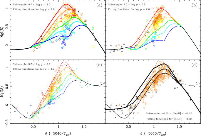
Figure 12: MgI values and general fitting functions for different atmospheric parameter regimes. Panels $a$, $b$ and $c$ display, respectively, all the stars with gravities in the ranges $0.0\leq\log g<2.0$, $2.0\leq\log g<3.2$ and $3.2\leq\log g<5.2$, together with the derived fitting functions for the mean gravity in each range, i.e., $\log g=$ 1.0 (a), 2.6 (b) and 4.2 (c). In the mid-temperature range, the different lines represent, from top to bottom, the functions for metallicities [Fe/H] = $+0.5$, 0.0, $-0.5$, $-1.0$, $-1.5$, and $-2.0$, whilst, for high and low temperatures, the fitting functions do not depend on metallicity. Panel $d$ shows all the stars around solar metallicity ($-0.25<{\rm[Fe/H]}\leq+0.25$) and the corresponding fitting functions computed for [Fe/H] = 0.0 and different values of gravity ($\log g$ = 0.0, 1.0, 3.0, and 5.0, from the thickest to the thinnest line). Codes and relative sizes of the star symbols (indicating, respectively, metallicity and gravity ranges) are explained in Fig. 9a. Note that, while the lines displayed here correspond to fitting functions at particular values of $\log g$ and [Fe/H], the plotted stars span a range of atmospheric parameters around these central values. This is the reason why the lines do not exactly fit all the points in the plots. Also, note that these fitting functions have not been derived by using only these plotted stars, but the whole sample.

At both ends of the temperature regime covered by our stellar library, MgI exhibits a different behaviour for dwarf stars, on one side, and giant and supergiants stars, on the other one. This is why we defined separate boxes in Table 5 to compute the corresponding local fits: $a$ and $b$, for hot dwarfs and giants; $e$ and $f$, for cold dwarfs and giants. No terms in $\log g$ and [Fe/H] were found to be statistically significant in any of the two luminosity bins, so only terms in $\theta$ were needed. However, for intermediate temperatures (warm and cool stars; boxes $c$ and $d$ in Table 5), the three atmospheric parameters play an important role to reproduce the complex behaviour of the MgI index.

Figures 12a, 12b, and 12c illustrate the general fitting functions (that is, the interpolation of all the local fitting functions) for three gravity bins, that typically represent supergiants, giants, and dwarfs, respectively. As expected, there exists a clear dependence on metallicity and $\theta$ at intermediate temperatures in the sense that MgI increases with the increasing [Fe/H] and the decreasing temperature. Figure 12d displays the derived fitting functions for solar metallicity and different gravity values. Apart from reinforcing the strong temperature dependence of the MgI index, this figure illustrates that gravity effects are not negligible at intermediate temperatures. As a matter of fact, there exists a sort of degeneracy in the sense that dwarf stars (thinest solid lines; $\log g\sim 4-5$) and supergiant stars (thickest solid lines; $\log g\sim 0-1$) reach similar MgI values, the ones are systematically larger than those of giants with intermediate $\log g$ values.

It is important to note that, while the lines in Figure 12 correspond to projections of the fitting functions at particular values of $\log g$ and [Fe/H], the plotted stars span a range of atmospheric parameters around these central values. Therefore, it is not expected the lines to fit exactly all the points in the plots. In any case, there are still some curves which do not appear to be well constrained by the observations in certain regions of the parameter space. For instance, there are no stars for $\theta<0.5$ in Figure 12a ($\log g=1.0$) and for $\theta>1.3$ in Figure 12b ($\log g=2.6$). Stars with these parameters just do not exist, and therefore they will never be required by the stellar populations models.

Because of the complicated functional form of MgI at intermediate temperatures as compared to that of cold stars, the local fit in Table 5d was specially designed to preserve smoothness when interpolating the local fits of warm and cold stars. Even so, a ficticious peak in the fitting functions of very metal-poor ([Fe/H] $\sim-2.0$) giants and supergiants at $\theta\sim 1.2$ is still apparent in Figures 12a,b. This is in part due to the lack of reliable metallicity determinations for very cold stars, which prevents us from a more accurate calibration of metallicity effects all over the $\theta$–$\log g$ space. As a matter of fact, there exists a stronger limitation arising from the intrinsic absence of metal-poor, very cold giant stars, as the red giant and asymptotic giant branches of so metal-poor populations —like, e.g., the globular cluster M92— do not reach so low temperatures. Once again, we are confident that the above interpolation is not having an important effect on the integrated MgI values computed for low-metallicity SSPs.

It is worth noting here that, aside from studying the behaviour of the Mg i line, DTT also calibrated the strength of the MgI(DTT) index as a function of the stellar atmospheric parameters. By performing a principal component analysis for the 106 stars of their library (F5 to M1 spectral types), they derived a biparametrical linear dependence on metallicity and effective temperature —with no sensitivity to surface gravity—, so that MgI(DTT) increases with the increasing [Fe/H] and the decreasing $T_{\rm eff}$. In spite of the parameter coverage of the DTT stellar sample allowing to detect the weak dependence on $\log g$ and other significant terms, they restricted their analysis to the two first principal components, what explains the simple dependence reported in their work. For this reason, the DTT calibration, although useful for achieving a first order understanding of the MgI behaviour, should not be considered as an accurate input ingredient for SSP modeling. As a matter of fact, a simple extrapolation of the DTT calibration to larger and lower temperatures fails to reproduce, among other, the observed MgI turnover at $\theta\sim 1.2$ (after which MgI decreases with the decreasing $T_{\rm eff}$) and the MgI plateu for the earliest spectral types.

3.2.3 sTiO fitting functions

Figure 13: sTiO values for all the stars around solar metallicity ($-0.25<{\rm[Fe/H]}\leq+0.25$). The curves correspond to general fitting functions computed for [Fe/H] = 0.0 and different values of gravity ($\log g$ = 0.0, 1.0, 3.0, and 5.0, from the thickest to the thinnest line). Codes and relative sizes of the star symbols (indicating, respectively, metallicity and gravity ranges) are explained in Fig. 9a.

As it was described in Section 3.1.3, the index sTiO exhibits values around 1 —or slightly smaller— for most library stars except for the latest spectral types, for which the index increases with the decreasing temperature. Boxes $d$, $e$, and $f$ in Table 6 were designed to reproduce, separately for dwarf and giant stars, the increasing sTiO trend at the low temperature regime. Only terms in $\theta$ were necessary, as it also happens for the earliest spectral types (boxes $a$ and $b$).

In spite of the apparent constancy of the sTiO values for intermediate temperatures, terms in all the three atmospheric parameters turned out to be statistically significant in box $c$, with the [Fe/H] dependence being the less important. For this reason, Figure 13 —for solar metallicity and different gravities— suffices to illustrate the general fitting functions of the sTiO index. Apart from the strong sTiO increase with the decreasing temperature (particularly for cold giant stars), it is worth noting the gravity effect at the intermediate temperature regime, in the sense that the larger the gravity (dwarfs; thinest solid lines), the lower the sTiO index.

3.3 Residuals and error analysis

Figure 14: Residuals of the MgI fitting functions ($\Delta{\rm MgI}={\rm MgI}_{\rm obs}-{\rm MgI}_{\rm pred}$) versus $\theta$ for the whole stellar library. See Fig. 9a for symbol codes. The error bar at the left margin indicates the unbiased residual standard deviation of the fit. See text in Sections 3.3 and  3.4 for a study on the different error sources driving the observed residuals.

Figure 15: Residuals of the sTiO fitting functions ($\Delta{\rm sTiO}={\rm sTiO}_{\rm obs}-{\rm sTiO}_{\rm pred}$) versus $\theta$ for the whole stellar library. See Fig. 9a for symbol codes. The error bar at the left margin indicates the unbiased residual standard deviation of the fit. See text in Section 3.3 for a study on the different error sources driving the observed residuals.

Defining the index residual of a given star as the difference between the observed index and the one predicted by the fitting functions ($\Delta{\cal I}={\cal I}_{\rm obs}-{\cal I}_{\rm pred}$), Figures 14 and 15 show the residuals of the indices MgI and sTiO for the whole stellar library as a function of $\theta$. These residuals are given for each star in Table 10. Overall, no systematic deviations are found for any of the three atmospheric parameters. Star clusters have also been analyzed separately and, except for the MgI values of the open cluster M67, no systematic effects have been found. We defer the analysis of this particular case to Section 3.4, where the effect of different [Mg/Fe] ratios on the MgI fitting function residuals is discussed.

Table 7: Statistical data for the general fitting functions of the indices MgI and sTiO. N: number of stars; $\sigma_{\rm std}$: unbiased residual standard deviation; $\sigma_{\rm typ}$: typical index error for the stars used in the fits; $r^{2}$: determination coefficient.

	N	$\sigma_{\rm std}$	$\sigma_{\rm typ}$	$r^{2}$
MgI	647	0.091	0.043	0.91
sTiO	668	0.017	0.004	0.97

Table 8: Uncertainties of the MgI and sTiO fitting functions for different subsets of stars, and mean index errors due to uncertainties in the flux calibration and the input atmospheric parameters. Open clusters are Coma, Hyades, M67, NGC188 and NGC7789. Globular clusters include M3, M5, M10, M13, M71, M92 and NGC6171. $N$: number of stars. $\sigma_{\rm typ}$: typical observational index error, accounting for photon noise and typical uncertainties in radial velocity. $\sigma_{T_{\rm eff}}$, $\sigma_{\log g}$ and $\sigma_{\rm[Fe/H]}$: mean index errors due to uncertainties in the input $T_{\rm eff}$, $\log g$ and [Fe/H]. $\sigma_{{\rm par}}$: total error due to atmospheric parameters (quadratic addition of the three previous ones). $\sigma_{\rm fcal}$: mean index error arising from random uncertainties in the flux calibration. $\sigma_{{\rm ALL}}$: total error due to all the above uncertainties (quadratic addition of $\sigma_{\rm typ}$, $\sigma_{{\rm par}}$, and $\sigma_{\rm fcal}$). $\sigma_{\rm std}$: unbiased residual standard deviation of the fit.

	Index	$N$		$\sigma_{\rm typ}$		$\sigma_{T_{\rm eff}}$	$\sigma_{\log g}$	$\sigma_{\rm[Fe/H]}$	$\sigma_{{\rm par}}$		$\sigma_{\rm fcal}$		$\sigma_{\rm ALL}$	$\sigma_{\rm std}$
Open clusters	MgI	92		0.065		0.037	0.009	0.056	0.068		0.007		0.094	0.114
	sTiO	93		0.006		0.003	0.001	0.001	0.003		0.011		0.013	0.017
Globular clusters	MgI	53		0.174		0.019	0.006	0.056	0.060		0.007		0.184	0.219
	sTiO	54		0.015		0.002	0.002	0.003	0.004		0.011		0.019	0.028
Field dwarfs	MgI	236		0.042		0.030	0.029	0.026	0.049		0.007		0.065	0.082
	sTiO	242		0.004		0.004	0.003	0.001	0.005		0.012		0.014	0.011
Field giants	MgI	196		0.036		0.026	0.009	0.028	0.039		0.007		0.054	0.091
	sTiO	204		0.003		0.017	0.004	0.001	0.017		0.012		0.021	0.016
Field supergiants	MgI	70		0.039		0.030	0.025	0.030	0.049		0.007		0.063	0.092
	sTiO	75		0.004		0.023	0.007	0.002	0.024		0.012		0.027	0.031
Hot stars ($0.13<\theta<0.69$)	MgI	67		0.040		0.054	0.014	0.023	0.061		0.007		0.073	0.086
	sTiO	68		0.004		0.010	0.003	0.000	0.011		0.011		0.016	0.022
Intermediate stars ($0.69<\theta<1.30$)	MgI	555		0.044		0.023	0.018	0.036	0.047		0.007		0.065	0.090
	sTiO	560		0.004		0.001	0.003	0.001	0.004		0.012		0.013	0.016
Cold stars ($1.30<\theta<1.84$)	MgI	25		0.029		0.061	0.009	0.006	0.062		0.007		0.069	0.106
	sTiO	40		0.004		0.123	0.004	0.002	0.123		0.022		0.125	0.025
All	MgI	647		0.043		0.029	0.018	0.034	0.048		0.007		0.065	0.091
	sTiO	668		0.004		0.009	0.003	0.001	0.010		0.012		0.016	0.017

To explore in more detail the reliability of the present fitting functions, in Table 7 we list the unbiased residual standard deviation from the fits, $\sigma_{\rm std}$, the typical error in the measured indices arising from photon noise and radial velocity uncertainties, $\sigma_{\rm typ}$, and the determination coefficient, $r^{2}$, for all the stars employed in the computation of the general fitting functions. It is important to note that, apart from the outlier stars rejected from the fits, a few stars with unknown [Fe/H] could not be included in the metallicity-dependent fits and no residuals were therefore computed. It is clear that, for both indices, $\sigma_{\rm std}$ is larger than what it should be expected uniquely from typical errors (see also the partial values of $\sigma_{\rm std}$ and $\sigma_{\rm typ}$ in Tables 5 and 6), what suggests that the fitting function residuals must be dominated by other effects. In CEN02 it was demonstrated that the errors in the input parameters were the main source of residuals for the fitting functions of the Ca ii indices. We therefore perform a similar analysis to constrain the effect of the atmospheric parameter uncertainties in the residuals of the MgI and sTiO fitting functions. Aimed at constraining the potential sensitivity of sTiO to small changes in the continuum shape, the effect of flux calibration uncertainties is also discussed.

3.3.1 Uncertainties in the stellar atmospheric parameters

We have computed how the errors in the input atmospheric parameter of the library stars translate into uncertainties in the predicted indices. Since this depends on both the local functional form of the fitting functions (e.g., a weak dependence on temperature leads to small index errors due to $T_{\rm eff}$ uncertainties) and the atmospheric parameters range (e.g., both hot and very cold stars have $T_{\rm eff}$ uncertainties larger than intermediate temperature stars), we have not only performed the analysis for the stellar library as a whole but also for different sets of stars (listed in Table 8).

For each star of the sample we have derived three index errors, arising from the corresponding uncertainties in $T_{\rm eff}$, $\log g$ and [Fe/H]. As input atmospheric parameters uncertainties we have made use of the values presented in Table 7 of CEN01b. Apart from those, we have used errors of 75 K, 0.40 dex and 0.15 dex for the effective temperatures, gravities and metallicities taken from Soubiran, Katz & Cayrel (1998) (with 4000 K $<T_{\rm eff}<$ 6300 K; stars coded skc in Table 6 of CEN01b), and 75 K, 0.05 dex and 0.20 dex for the cluster stars. For each subset of stars we have computed a mean index error as a result of the uncertainty of each parameter ($\sigma_{T_{\rm eff}}$, $\sigma_{\log g}$ and $\sigma_{\rm[Fe/H]}$) by using the input parameter errors for all the individual stars. Finally, an estimate of the total expected error due to atmospheric parameters ($\sigma_{{\rm par}}$) is computed as the quadratic addition of the three previous errors.

It is clear from the data in Table 8 that $\sigma_{{\rm par}}$ is, in all cases, comparable or larger than $\sigma_{{\rm typ}}$. This result reinforces the importance of using an homogeneous and reliable set of atmospheric parameters to guarantee the accuracy of this kind of calibrations. Also, it is interesting to see how $\sigma_{T_{\rm eff}}$ for cold stars is much larger than their observed dispersion w.r.t. the fits, $\sigma_{\rm std}$. This would mean that the error in $T_{\rm eff}$ quoted in CEN01b for this types of stars was somewhat overestimated.

Table 9: Absolute errors in the fitting functions predictions for different values of the atmospheric parameters. Input $\log g$ values varying with effective temperature for dwarfs, giants and supergiants have been taken from Lang (1991). Since, for extreme temperatures, the fitting functions do not depend on metallicity, no [Fe/H] value has been adopted for 15000 K and 3200 K. This is also the case for some values at 3500 K.

		dwarfs		giants		supergiants
$T_{\rm eff}$	[Fe/H]	$\Delta$sTiO	$\Delta$MgI	$\Delta$sTiO	$\Delta$MgI	$\Delta$sTiO	$\Delta$MgI
15000		0.001	0.041	0.001	0.041	0.007	0.029
8000	$+$0.5	0.002	0.031	0.002	0.031	0.007	0.039
8000	0.0	0.002	0.029	0.002	0.031	0.007	0.039
8000	$-$1.0	0.003	0.034	0.002	0.034	0.007	0.042
8000	$-$2.0	0.003	0.082	0.003	0.080	0.007	0.082
6000	$+$0.5	0.003	0.023	0.004	0.023	0.006	0.033
6000	0.0	0.002	0.013	0.003	0.016	0.006	0.029
6000	$-$1.0	0.003	0.018	0.004	0.021	0.006	0.033
6000	$-$2.0	0.006	0.048	0.005	0.048	0.007	0.054
5000	$+$0.5	0.005	0.045	0.003	0.031	0.006	0.038
5000	0.0	0.004	0.031	0.002	0.016	0.005	0.028
5000	$-$1.0	0.004	0.032	0.003	0.022	0.005	0.029
5000	$-$2.0	0.007	0.048	0.005	0.038	0.007	0.039
4000	$+$0.5	0.006	0.063	0.005	0.064	0.009	0.078
4000	0.0	0.006	0.051	0.004	0.037	0.008	0.063
4000	$-$1.0	0.006	0.052	0.004	0.055	0.007	0.066
4000	$-$2.0	0.007	0.084	0.007	0.120	0.009	0.114
3500	$+$0.5	0.010	0.045	0.027	0.072	0.027	0.073
3500	0.0	0.010	0.044	0.027	0.067	0.027	0.068
3500	$-$1.0	0.010	0.046	0.027	0.080	0.027	0.081
3500	$-$2.0	0.010	0.050	0.027	0.104	0.027	0.103
3200		0.011	0.041	0.042	0.063	0.042	0.063

Furthermore, since the aim of this paper is to predict reliable index values for any combination of input atmospheric parameters, we have also computed the random errors in such predictions making use of the covariance matrices of the fits. These uncertainties are given in Table 9 for some representative values of input parameters. Note that, as it is expected, the absolute errors are larger for cold giants and supergiants and, in general, increase as the metallicity departs from the solar value. These errors are the ones provided by the fortran routine that computes the fitting function predictions as uncertainties of the output MgI and sTiO indices.

3.3.2 Uncertainties in the flux calibration

An additional source of index errors that may increase the fitting function residuals is the uncertainty in the flux calibration of the library stars. At this point, we are not interested in the quality of the flux calibration in an absolute sense, as any minor departure from the “true” calibration must be considered as a systematic that applies to the stellar library as a whole, and hence it would not affect the fitting function residuals. Instead, we aim at constraining the random errors in the final flux calibration curve and their effects on the index measurements.

It is important to note that, in CEN01a, all the stars of a given observing run were flux calibrated by applying one response curve, the one that was obtained as an average of all the individual response curves derived from single observations of spectrophotometric standard stars (10 – 20 per observing run). Therefore, using each of the above individual curves to re-calibrate the stellar spectra, we repeated the index measurements for all the stars to estimate a random error, arising from flux calibration uncertainties ($\sigma_{\rm fcal}$), as the r.m.s. standard deviation of all the individual index measurements.

The above procedure allowed us to confirm that, as expected (see Section 2.4.3), and unlike MgI, sTiO is very sensitive to flux calibration. On average over all the different observing runs, we obtain that $\sigma_{\rm fcal}\sim 0.012\times$ sTiO, what turns the flux calibration uncertainty into the main source of random error of the index sTiO (much larger than the joint effect of photon noise and radial velocity uncertainty). With typical sTiO values in the range 0.90 – 0.95, the majority of hot and intermediate $T_{\rm eff}$ stars ($T_{\rm eff}\ga 3900$ K; $\theta\la 1.30$ K^-1) have $\sigma_{\rm fcal}\sim 0.011$. Colder stars, however, having a much larger sTiO values, reach errors of up to $\sigma_{\rm fcal}\sim 0.031$. According to the averaged sTiO values of the distinct categories of stars, different $\sigma_{\rm fcal}$ values for sTiO are given in Table 8. In addition, a typical value of $\sigma_{\rm fcal}=0.007$ Å for MgI has been derived from all the library stars.

3.3.3 Overall random uncertainties

The quadratic addition of $\sigma_{\rm typ}$, $\sigma_{\rm par}$ and $\sigma_{\rm fcal}$ can be interpreted as an overall random uncertainty, $\sigma_{\rm ALL}$, which is computed and listed for each group of stars in Table 8. Note that, unlike to what happens for $\sigma_{\rm typ}$, the new $\sigma_{\rm ALL}$ values account for most of (or even all) the dispersion of the fits, $\sigma_{\rm std}$. In other words, the residuals of the fits are consistent with the expected scatter due to the individual index errors. This is particularly true for sTiO, with $\sigma_{\rm ALL}=0.016$ and $\sigma_{\rm std}=0.017$ for the whole stellar library. However, it seems that an additional source of error is still needed to reconcile $\sigma_{\rm ALL}$ and $\sigma_{\rm std}$ for MgI. This point is addressed in more detail in Section 3.4.

3.4 [Mg/Fe] abundance ratios

Figure 16: [Mg/Fe] abundance ratios vs [Fe/H] for 196 stars of the library in CEN01a. Different symbols and sizes indicate metallicities and gravities as in Fig. 9a. The solid line is the least-squares fit to the data given in Eq. 10.

Figure 17: Residuals of the MgI fitting functions ($\Delta$MgI; observed – predicted) vs residuals w.r.t. the intrinsic [Mg/Fe]–[Fe/H] relation of the stellar library (Eq. 10; Figure 16). Symbols and sizes as in Fig. 9a. The solid line represents an error-weighted least-squares linear fit to all points within 3$\sigma$ r.m.s.

Given that MgI is a Mg i index, in principle one would expect its metallicity dependence to be better described in terms of the Mg abundance, [Mg/H], rather than [Fe/H]. In this section we constrain the importance of different [Mg/Fe] ratios on driving the strength of the MgI index.

To do this analysis, we have compiled [Mg/Fe] data from the literature for 196 library stars. Most data were taken from the catalogue of Borkova & Marsakov (2005), as they performed a previous compilation of [Mg/Fe] data in the literature and, then, corrected the different sources from systematics to end up with an homogeneous [Mg/Fe] system. In addition, for a few stars which were not available in the above catalogue, we included the data from Gratton & Sneden (1987), Pilachowski, Sneden & Kraft (1996), and Thévenin (1998). The later, having a large number of stars in common with Borkova & Marsakov, was previously transfomed into the Borkova & Marsakov’s system by using all the stars in common between both catalogues.

Since our stellar library mainly consists of nearby stars, it matches the well-known [Mg/Fe]-[Fe/H] pattern of the solar neighbourhood (e.g. Edvardsson et al. 1993), in the sense that [Mg/Fe] decreases with the increasing [Fe/H]. Figure 16 illustrates such a trend for the 196 library stars with available data. Far from being well represented by just a linear relationship, a least-squares polynomial fit to all the stars in Fig. 16 gives

$$\begin{array}[]{l}{\rm[Mg/Fe]}_{0}=0.08(\pm 0.01)-0.33(\pm 0.04)~{}{\rm[Fe/H]}\\ \vskip 6.0pt plus 2.0pt minus 2.0pt\cr-0.13(\pm 0.04)~{}{\rm[Fe/H]}^{2}-0.02(\pm 0.01)~{}{\rm[Fe/H]}^{3},\end{array}$$ (10)

where [Mg/Fe]₀ can be considered as the averaged [Mg/Fe] ratio of the solar neighbourhood. Note that such a relationship is implicitly taken into account in the fitting functions through the adopted [Fe/H] and, therefore, a systematic trend between the MgI fitting functions residuals and the [Mg/Fe] ratios should not be expected. We have therefore investigated whether the residuals of the MgI fitting functions for individual stars ($\Delta{\rm MgI}$; as defined in Section 3.3) are correlated with their deviations from Eq. 10 ($\Delta{\rm[Mg/Fe]}\equiv{\rm[Mg/Fe]}-{\rm[Mg/Fe]}_{0}$). Figure 17 confirms that there is indeed a significant relation between $\Delta{\rm MgI}$ and $\Delta{\rm[Mg/Fe]}$, in the sense that stars with larger Mg abundances (at fixed [Fe/H]) tend to have positive residuals in the MgI fitting functions. An error-weighted linear fit to this trend gives

$$\begin{array}[]{l}{\Delta{\rm MgI}=0.005(\pm 0.006)+0.27(\pm 0.09)~{}\Delta{\rm[Mg/Fe]}.}\end{array}$$ (11)

An immediate implication of the above correlation is that it must account for part of the unexplained MgI residuals reported in Section 3.3.3. In fact, the variance of the fit in Eq. 11 is $\sim 10$ percent smaller than $\sigma^{2}_{\rm std}$ of MgI for the stars in Fig. 17. If this subsample were representative of the whole library, different [Mg/Fe] ratios might explain $\sim 0.029$ Å of the total MgI $\sigma_{\rm std}$ (0.091 Å). As a matter of fact, this number must be considered as a lower limit since cluster stars do not necessarily follow the [Mg/Fe] pattern of field stars (see Section 3.4.1) and larger MgI residuals are expected for this subsample of stars. In addition, the existence of the correlation given in Eq. 11 demonstrates that the MgI index is indeed a good indicator of the Mg abundance. Note that this is not necessarily true for all metal-line indices, as it was demonstrated in CEN02 that the Ca ii triplet indices do not depend on minor changes in [Ca/Fe].

Unfortunately, [Mg/Fe] ratios are only available for less than one-third of the library stars. Even though this number is large enough to perform a reliable analysis as the one presented above, it is not worthy trying to include a [Mg/Fe] term in our fitting functions, as not only the small number of stars but also the more limited atmospheric parameter coverage of the subsample would dramatically affect the accuracy and reliability of the empirical calibration. Instead, we prefer to keep the fitting functions in their present form and stress the idea that, by being constrained to the chemical enrichment of the solar neighborhood, they are subject to exhibit systematics with respect to other enrichment scenarios in which Mg abundances are well different.

3.4.1 The MgI residual of M67

Figure 18: MgI residuals ($\Delta$MgI; observed – predicted) vs $\log g$ for M67 stars. A significant offset of $\Delta{\rm MgI}=-0.134\pm 0.022$ Å is observed.

Compared to the predictions of the MgI fitting functions, M67 stars show a significant mean offset of $\Delta{\rm MgI}=-0.134\pm 0.022$ Å that cannot be solely explained by typical random errors. Figure 18 illustrates the derived offsets for all the 20 stars in M67.

Given that the sensitivity of MgI to $\log g$ is relatively small as compared to other atmospheric parameters, small uncertainties in the distance moduli adopted by the original references that derived surface gravities (see CEN01b) are not expected to be responsible for the observed discrepancy. Instead, since MgI increases with metallicity, the negative MgI residual of M67 could be explained if the true cluster metallicity were lower than the value adopted in this work ([Fe/H] $=-0.09$, from Friel & Janes 1993; see CEN01b). In this sense, according to our fitting function predictions, a cluster metallicity of [Fe/H] $\sim-0.32$ would suffice to make the offset statistically non-significant given the MgI errors of the M67 stars. However, aside the pioneering work by Cohen (1980) in which an averaged value of [Fe/H] $=-0.39$ was reported for M67, more recent work derived roughly solar (or slightly below solar) iron abundances for the cluster stars, like e.g. $-0.1\pm 0.1$ (Foy & Proust 1981), $-0.09\pm 0.07$ (Friel & Janes 1993), $-0.15\pm 0.05$ (Friel et al. 2002), $-0.03\pm 0.03$ (Tautvaisiene et al. 2000), $+0.02\pm 0.06$ (Gratton 2000). Therefore, assuming that the adopted value is a reasonable compromise for the [Fe/H] of the cluster, and keeping in mind that MgI indeed depends on the Mg abundance, the MgI residual could be a natural consequence of [Mg/Fe] differences between M67 stars and field stars at similar [Fe/H].

As regards to the [Mg/Fe] value of M67, there seems to exist some discrepancy in the literature. For instance, Tautvaisiene et al. (2000) reported [Mg/Fe] $\sim+0.1$ for evolved (giant and clump) stars in M67, whilst an error-weighted mean of the values presented by Shetrone & Sandquist (2000) for a sample of turn-off stars and blue stragglers in the cluster gives [Mg/Fe] $=-0.14\pm 0.10$.

Making use of Eq. 10, it is easy to convert [Fe/H] into [Mg/H] abundances to test the above hypothesis. At [Fe/H] $=-0.09$ (the metallicity adopted for M67), field library stars have an average value of [Mg/H] $=+0.02$ ([Mg/Fe] $=+0.11$), whereas at [Fe/H] $=-0.32$ (the value at which the MgI residual would not be significant), [Mg/H] $=-0.13$ ([Mg/Fe] $=+0.19$). This implies that, if MgI is indeed driven by Mg rather than Fe, the MgI residual of M67 could be explained if the Mg content of its stars were offset by $\Delta$[Mg/H] $=-0.15$ with respect to that of field stars. In other words, keeping [Fe/H] $=-0.09$ for M67, a value of [Mg/Fe] $\sim-0.04$ for M67 is required to account for the MgI residuals. This value is in good agreement with the work by Schiavon, Caldwell & Rose (2004), which constrains the [Mg/Fe] of M67 between $-0.1$ and $0.0$ on the basis of the integrated Mg$b$ in the cluster spectrum. Also, it is consistent with previous result from Friel & Janes (1993) that the metallicity derived for M67 from Mg$b$ is significantly lower than the one inferred from Fe indices. We therefore conclude that the MgI residual of M67 is probably driven by the existence of a Mg underabundance of [Mg/Fe] $\sim-0.04$, in contrast with the averaged value [Mg/Fe] $\sim+0.11$ for field library stars of equal [Fe/H].

4 A comparison with theoretical work

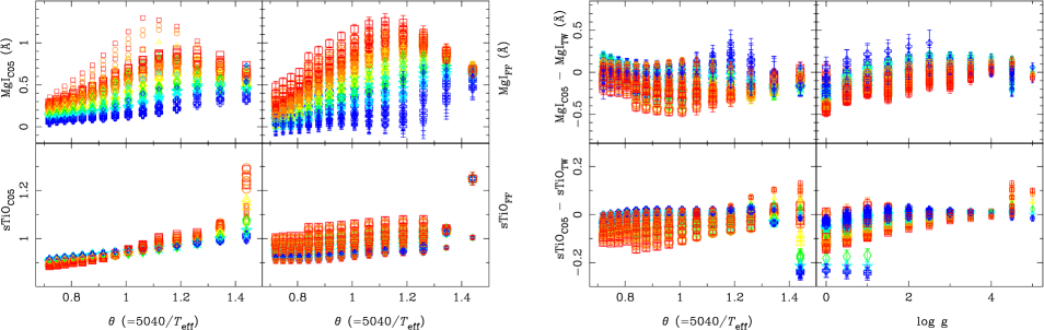
Figure 19: Left four panels: A comparison between the MgI and sTiO indices measured for the synthetic stars of Coelho et al. (2005; C05) and those predicted by the fitting functions (FF) of this paper at exactly the same atmospheric parameters of the synthetic stars. Right four panels: Star-by-star differences between the C05 and FF indices versus $\theta$ and $\log g$. For each index, vertical scales have been set to the same relative ranges of left panels to allow direct comparisons. Symbol types and relative sizes (indicating, respectively, metallicity and gravity ranges) are given as in Fig. 9a. See more details in the text.

We here provide a qualitative comparison between the new fitting functions presented in this paper and the MgI and sTiO predictions derived from theoretical work based on model atmospheres, in particular from the high-resolution synthetic stellar spectral library of Coelho et al. (2005; hereafter C05). This theoretical library ranges from the near-ultraviolet to the near-infrared, spaning the atmospheric parameter range of $3500\leq T_{\rm eff}\leq 7000$ K, $0.0\leq\log g\leq 5.0$ dex, and $-2.5\leq$[Fe/H]$\leq+0.5$ dex, at two different $\alpha$-element abundance ratios, [$\alpha$/Fe] = 0.0 and $+0.4$.

Prior to measuring the MgI and sTiO indices over the C05 stellar spectra, we smoothed and rebinned the C05 stellar spectra to match the spectral resolution and linear dispersion of the stars in CEN01a (FWHM$=1.5$ Å; 0.85 Å/pix). Also, for the sake of carrying out a meaningful comparison with our predictions, we removed from the current analysis all those synthetic stars that, because of their atmospheric parameters, are not expected to be required by SSP codes. This includes, for instance, late spectral types with intermediate surface gravity values (e.g. from $T_{\rm eff}=4500$ K and $\log g=4$ dex, down to $T_{\rm eff}=3500$ K and $1.5\leq\log g\leq 4$ dex), and hot dwarfs with very high surface gravity values ($T_{\rm eff}\geq 5000$ K and $\log g=5$). This way we also guaranteed that the overall atmospheric parameter space of the synthetic stars is not very different from that covered by the real stars in CEN01a.

To avoid systematics between the MgI of both samples arising from the existence of different Mg abundances at fixed [Fe/H], we took into account the [Mg/Fe]-[Fe/H] abundance pattern of the stars in CEN01a (see Section 3.4) and corrected the C05 indices for this effect. To do this, for each [Fe/H] value in C05 we determined its corresponding [Mg/Fe] according to Eq. 10. Hence, the final MgI and sTiO indices for the synthetic C05 stellar spectra are the result of interpolating linearly the indices measured at [$\alpha$/Fe] = 0.0 and 0.4 according to the above [Mg/Fe] value.

With all the considerations given above, the four left panels in Figure 19 illustrate a comparison between the MgI and sTiO indices measured on the C05 synthetic stars and those derived from our MgI and sTiO fitting functions for exactly the same atmospheric parameters of the synthetic stars. Although there exists a reasonable qualitative agreement in the first order behaviours of both datasets, absolute numbers reveal significant differences between real and synthetic indices. This is more clearly presented in the four right panels of Fig. 19, where the star-by-star absolute differences are plotted versus $\theta$ and $\log g$. The r.m.s. standard deviation of the index differences are $\sigma_{{\rm std}}=0.142$ Å and 0.042 for MgI and sTiO respectively, much larger than the typical residuals in Table 7 and Figs. 14 and 15. Some of these differences may be due to the limitation of our fitting functions to reproduce the poorly populated regions of the parameter space (e.g. the MgI of metal-poor stars at $\theta\sim 1.2$; see discussion in Section 3.2.2). However, most cases can not be justified in this way (e.g. synthetic MgI and sTiO indices do not to reproduce satisfactorily the gravity dependence exhibited by real stars, particularly for intermediate-to-high metallicity giants) and the intrinsic limitations of theoretical model atmospheres hence appear as potential sources for the observed differences. It is not however the scope of this section to provide a detailed analysis of the origins for the observed differences but to illustrate the reader with a comparative analysis between theoretical and empirical work. A similar comparison for the Ca ii triplet lines can be found in Vazdekis et al. (2003).

5 Summary and conclusions

Based on the near-IR stellar library of CEN01a,b we have defined new line-strength indices for the MgI line at 8807 Å and the TiO bands around the Ca ii triplet region. These indices, called MgI and sTiO respectively, are thought to be used as stellar population diagnostics. For this reason, we have characterized their sensitivities to different signal-to-noise ratios, distinct spectral resolutions, flux calibration and reddening correction systematics, and the presence of sky line residuals typical of this spectral range. Also, we give some recipes for those readers interested in transforming their old MgI and TiO index data into our new system of indices.

After measuring MgI and sTiO for all the library stars at the spectral resolution of CEN01a, we have calibrated their dependences on the stellar atmospheric parameters ($T_{\rm eff}$, $\log g$ and [Fe/H]) by means of empirical fitting functions. The reliability and accuracy of the new fitting function predictions have been discussed by performing a thorough analysis of the different error sources driving the fitting function residuals. For sTiO, these residuals are overall compatible with the ones expected from the uncertainties in the input atmospheric parameters and from the random errors in the index measurements (accounting for photon noise, radial velocity uncertainties, and flux calibration errors). For MgI, however, an additional contribution to the fitting function residuals arises from the existence of distinct [Mg/Fe] ratios among the library stars. As a consequence of this analysis, we have detected a statistically significant offset in the MgI values of M67 stars. This is consistent with M67 having a [Mg/Fe] underabundance of $\sim-0.04$, in contrast with the typical [Mg/Fe]$\sim+0.11$ of solar-neighbourhood stars with the same [Fe/H].

A full database with the index measurements for each library star, their random errors, the fitting function residuals, and the compiled [Mg/Fe] values is given in Table 10. This database, together with the FORTRAN routine for the evaluation of the fitting functions, are also available at
http://www.ucm.es/info/Astrof/ellipt/MgIsTiO.html
In a forthcoming paper (Vazdekis et al. in preparation), SSP model predictions for MgI and sTiO will be presented on the basis of such fitting functions, either at the above website and at A. Vazdekis models website.

To conclude, a brief summary of the main characteristics of the indices, their behaviours, and their potential capabilities for stellar population studies is given below:

• MgI has been specifically designed to be a very sensitive indicator of Mg abundance. For this reason, because of its relatively narrow line bandpass, it turns out to be dependent on the overall spectral resolution (and, hence, on the velocity dispersion of galaxies). Users are therefore encouraged to put their data into a homogeneous system of spectral resolution (either using the sigma-dependent polynomials provided in Table 3, or broadening their spectra up to a common overall spectral resolution) before any meaningful comparison of the MgI index among different types of objects.

  MgI exhibits a complex dependence on the three main stellar atmospheric parameters. For hot and cold stars, $T_{\rm eff}$ and $\log g$ are the main driving parameters, whereas, in the mid-temperature regime ($4000\leq T_{\rm eff}\leq 7000$ K), all three parameters play a significant role: MgI increases with the increasing metallicity and the decreasing temperature, with a mild dependence on the luminosity class that makes dwarfs and supergiant stars to exhibit slightly larger MgI values than giant stars.

  For stellar populations studies, as it will be shown in a forthcoming paper (Vazdekis et al. in prep.), the integrated MgI turns out to be an excellent indicator of the Mg abundance.

• The sTiO index has been defined to measure the slope of the pseudo-continuum of the Ca ii triplet region, which is known to change dramatically for M-type stars due to the appearence of strong TiO molecular bands. Because of its definition, the sTiO index is strikingly robust against changes in spectral resolution —and velocity dispersions— and low S/N ratios, which makes it particularly suited for the analysis of galaxies at high redshifts and extragalactic globular clusters. It however requires the spectra to have a proper relative flux calibration.

  As regards to the behaviour of sTiO in stars, it is worth noting the steep increase with the decreasing temperature for $T_{\rm eff}\leq 3600$ K. In turn, at such low temperatures, giant stars exhibit much stronger sTiO values than dwarfs, what makes sTiO to be a powerful dwarf-to-giant discriminator for M-type stars. In addition, the dependence of sTiO on the stellar metallicity is almost negligible.

  For the integrated spectra of quiescent galaxies, however, sTiO is found to reflect the overall metallicity of the stellar population, as the red giant branch gets cooler with the increasing metallicity and the relative contribution of M-type stars increases (see Vazdekis et al. 2003).

In Cenarro et al. (2003), both MgI and sTiO were measured for the first time over a sample of 35 elliptical galaxies, illustrating the usefulness of the MgI index to reproduce the Mg-$\sigma$ relation of elliptical galaxies at the near-IR, and the capabilities of sTiO as metallicity indicator.

Table 10: MgI and sTiO index measurements ($\cal I$), typical observational index error ($\sigma_{\rm typ}\cal I$, accounting for photon noise and typical uncertainties in radial velocity), fitting function residuals ($\Delta\cal I$), and [Mg/Fe] abundances (when available) for all the stars in CEN01a. Sources for [Mg/Fe] values are: (1) the catalogue of spectroscopic abundances in stars (Borkova & Marsakov 2005); (2) the catalogue of chemical abundances in late-type stars (Thevenin 1998) corrected to the Borkova & Marsakov (2005) system; (3) Pilachowski, Sneden & Kraft (1996); and (4) Gratton & Sneden (1987). The first five columns indicates the star number within the library, the name, the coordinates (RA and Dec in J2000, except M71 stars wich are B1950), and the spectral type and luminosity class. Additional information for the library stars (e.g. atmospheric parameters, [Ca/Fe] abundances, CaT, PaT, and CaT^∗ index values, their errors and fitting function residuals, $B$ and $V$ apparent magnitudes, signal-to-noise ratios per angstrom, and other names) can be found at CEN01a,b and at http://www.ucm.es/info/Astrof/ellipt/MgIsTiO.html.

Num	Name	RA	Dec	SpT	MgI(Å)			sTiO			[Mg/Fe]
		(h:m:s)	(d:m:s)		$\cal I$	$\sigma_{\rm typ}\cal I$	$\Delta\cal I$	$\cal I$	$\sigma_{\rm typ}\cal I$	$\Delta\cal I$
001	Coma A 3	12:19:16.7	$+$25:26:11	G9 V	0.417	0.097	$-$0.430	0.900	0.008	$-$0.025
002	Coma A 13	12:24:06.2	$+$26:07:44	K0 V	0.388	0.135	$-$0.318	0.865	0.010	$-$0.053
003	Coma A 14	12:24:17.6	$+$24:19:32	G4 V	0.396	0.080	$-$0.297	0.920	0.007	$-$0.002
004	Coma A 21	12:30:14.8	$+$25:01:44	G7 V	0.570	0.099	$-$0.185	0.919	0.008	$-$0.005
005	Coma T 65	12:19:28.3	$+$24:17:03	G0 V	0.285	0.079	$-$0.143	0.896	0.006	$-$0.017
006	Coma T 68	12:19:50.6	$+$28:27:51	A6 IV-V	$-$0.064	0.066	$-$0.008	0.920	0.005	$-$0.016
007	Coma T 82	12:21:26.7	$+$24:59:49	A9 V	$-$0.214	0.072	$-$0.257	0.893	0.005	$-$0.025
008	Coma T 85	12:21:49.0	$+$26:32:57	G1 V	0.487	0.062	0.049	0.904	0.005	$-$0.008
009	Coma T 86	12:21:56.2	$+$27:18:34	F6 V	0.068	0.071	$-$0.202	0.888	0.006	$-$0.024
010	Coma T 90	12:22:24.8	$+$22:27:51	F5 V	0.100	0.071	$-$0.183	0.886	0.006	$-$0.026
011	Coma T 97	12:23:08.4	$+$25:51:05	F9 V	0.462	0.084	0.068	0.906	0.007	$-$0.006
012	Coma T 102	12:23:42.2	$+$26:36:08	G1 V	0.338	0.122	$-$0.123	0.896	0.010	$-$0.017
013	Coma T 114	12:25:22.5	$+$23:13:45	F8 V	0.297	0.073	0.037	0.892	0.006	$-$0.019
014	Coma T 132	12:27:06.1	$+$26:50:47	G5 V	0.598	0.096	0.017	0.877	0.008	$-$0.037
015	Coma T 150	12:29:41.1	$+$24:31:13	G9 V	0.465	0.080	$-$0.213	0.889	0.006	$-$0.033
016	Hya vB 10	04:06:16.1	$+$15:41:53	G0 V	0.501	0.071	0.024	0.912	0.006	0.002
017	Hya vB 15	04:14:32.3	$+$23:34:30	G3 V	0.484	0.068	$-$0.100	0.913	0.006	$-$0.001
018	Hya vB 17	04:14:25.7	$+$14:37:30	G5 V	0.702	0.077	0.052	0.918	0.007	0.006	+0.05 2
019	Hya vB 19	04:14:34.3	$+$10:42:05	F8 V	0.360	0.062	0.006	0.909	0.005	$-$0.002
020	Hya vB 21	04:16:33.5	$+$21:54:26	K0 V	0.778	0.095	$-$0.011	0.917	0.008	0.000
021	Hya vB 26	04:18:58.0	$+$19:54:24	G9 V	0.706	0.079	0.018	0.924	0.007	0.010
022	Hya vB 31	04:20:13.0	$+$19:14:00	G0 V	0.370	0.067	$-$0.068	0.908	0.006	$-$0.003
023	Hya vB 35	04:21:31.7	$+$21:02:23	F5 V	0.224	0.040	$-$0.038	0.911	0.003	0.001
024	Hya vB 36	04:21:32.3	$+$18:25:03	F6 V	0.192	0.041	$-$0.069	0.907	0.003	$-$0.003
025	Hya vB 37	04:21:34.8	$+$14:24:35	F5 V	0.253	0.036	0.033	0.910	0.003	$-$0.001	+0.07 2
026	Hya vB 63	04:26:24.6	$+$16:51:12	G1 V	0.483	0.056	$-$0.036	0.921	0.005	0.007
027	Hya vB 64	04:26:40.1	$+$16:44:49	G2 V	0.569	0.061	$-$0.003	0.910	0.005	$-$0.003
028	Hya vB 73	04:28:48.3	$+$17:17:08	G2 V	0.540	0.062	0.047	0.902	0.005	$-$0.009	+0.11 2
029	Hya vB 81	04:30:18.0	$+$19:50:26	F6 V	0.369	0.044	0.064	0.912	0.004	0.002	+0.05 2
030	Hya vB 87	04:31:15.7	$+$20:07:59	G8 V	0.718	0.060	0.033	0.919	0.005	0.004
031	Hya vB 95	04:33:50.9	$+$14:50:40	A8 V n	0.002	0.049	$-$0.023	0.912	0.004	$-$0.014
032	Hya vB 103	04:38:09.4	$+$16:02:00	F0 V	0.161	0.045	0.062	0.917	0.004	0.001
033	Hya vB 104	04:38:09.5	$+$12:30:39	A6 V n	0.223	0.049	0.334	0.961	0.004	0.008
034	Hya vB 111	04:44:25.8	$+$11:08:46	F0 V	0.381	0.059	0.348	0.942	0.005	0.017
035	Hya vB 112	04:46:01.7	$+$11:42:20	Am	0.115	0.054	0.135	0.962	0.005	0.027
036	Hya vB 126	04:54:58.4	$+$19:29:07	F3 IV	0.043	0.034	$-$0.046	0.919	0.003	0.003
037	Hya vB 140	04:24:43.2	$+$04:42:00	G5 V	0.730	0.058	0.020	0.922	0.005	0.006
038	M10 II-76	16:56:51.3	$-$04:01:27	AGB	$-$0.057	0.194	$-$0.418	0.941	0.016	$-$0.016
039	M10 III-85	16:56:56.7	$-$04:11:12	GB	0.512	0.106	0.072	0.961	0.010	$-$0.008
040	M13 A 171	16:41:19.6	$+$36:21:15	AGB	0.585	0.116	0.160	0.958	0.010	$-$0.011
041	M13 B 786	16:41:23.5	$+$36:30:17	GB	0.336	0.108	$-$0.349	0.962	0.010	$-$0.028
042	M13 B 818	16:41:29.8	$+$36:31:56	AGB	0.574	0.230	0.335	0.949	0.020	0.014
043	M3 398	13:42:32.0	$+$28:27:03	GB	0.177	0.208	$-$0.227	0.923	0.016	$-$0.038
044	M3 III-28	13:41:45.8	$+$28:25:00	GB	0.530	0.137	$-$0.094	0.924	0.011	$-$0.065
045	M3 IV-25	13:41:36.3	$+$28:21:24	GB	0.507	0.183	0.036	0.940	0.015	$-$0.030
046	M5 I-45	15:18:41.5	$+$02:06:54	HB	0.368	0.188	0.207	0.913	0.016	$-$0.012
047	M5 II-51	15:18:21.1	$+$02:06:58	GB	0.186	0.251	$-$0.248	0.920	0.020	$-$0.038
048	M5 II-53	15:18:24.6	$+$02:06:57	HB	$-$0.306	0.298	0.030	0.982	0.026	0.006
049	M5 II-76	15:18:22.5	$+$02:07:29	HB	$-$0.096	0.246	$-$0.208	0.891	0.019	$-$0.032
050	M5 III-03	15:18:17.0	$+$02:04:54	GB	0.339	0.225	$-$0.397	0.956	0.020	$-$0.041

Table 10: Continuation

Num	Name	RA	Dec	SpT	MgI(Å)			sTiO			[Mg/Fe]
		(h:m:s)	(d:m:s)		$\cal I$	$\sigma_{\rm typ}\cal I$	$\Delta\cal I$	$\cal I$	$\sigma_{\rm typ}\cal I$	$\Delta\cal I$
051	M5 IV-19	15:18:33.1	$+$02:01:18	GB	0.266	0.232	$-$0.417	0.920	0.019	$-$0.070
052	M5 IV-59	15:18:44.0	$+$02:04:36	GB	0.573	0.197	$-$0.054	0.946	0.018	$-$0.043
053	M5 IV-86	15:18:43.0	$+$02:01:49	HB	0.228	0.202	0.022	0.924	0.017	$-$0.004
054	M5 IV-87	15:18:44.2	$+$02:01:52	HB	0.146	0.127	0.009	0.936	0.011	0.012
055	M67 F 084	08:51:12.7	$+$11:52:42	HB	0.620	0.061	$-$0.092	0.926	0.005	$-$0.032
056	M67 F 094	08:51:15.4	$+$11:50:14	SGB	$-$0.078	0.226	$-$0.374	0.873	0.017	$-$0.042
057	M67 F 105	08:51:17.1	$+$11:48:16	GB	0.655	0.073	$-$0.142	0.934	0.006	$-$0.032
058	M67 F 108	08:51:17.4	$+$11:45:24	GB	0.627	0.088	$-$0.226	0.954	0.008	$-$0.024
059	M67 F 115	08:51:18.6	$+$11:49:22	SGB	0.037	0.193	$-$0.310	0.864	0.014	$-$0.053
060	M67 F 117	08:51:18.7	$+$11:47:03	SGB	0.198	0.154	$-$0.365	0.897	0.012	$-$0.029
061	M67 F 119	08:51:19.0	$+$11:50:06	SGB	0.303	0.180	$-$0.019	0.904	0.014	$-$0.012
062	M67 F 125	08:51:20.2	$+$11:52:48	SGB	0.244	0.251	$-$0.106	0.912	0.019	0.000
063	M67 F 164	08:51:29.0	$+$11:50:33	HB	0.798	0.109	0.072	0.910	0.009	$-$0.050
064	M67 F 170	08:51:29.9	$+$11:47:17	GB	0.717	0.074	$-$0.133	0.947	0.007	$-$0.031	$-$0.08 2
065	M67 F 175	08:51:31.2	$+$11:53:18	SGB	0.055	0.239	$-$0.321	0.913	0.019	0.001
066	M67 F 193	08:51:35.8	$+$11:53:35	GB	0.549	0.125	$-$0.121	0.926	0.011	$-$0.014
067	M67 F 224	08:51:43.8	$+$11:44:26	GB?	0.512	0.100	$-$0.207	0.963	0.009	0.008
068	M67 F 231	08:51:45.1	$+$11:47:46	GB	0.598	0.089	$-$0.079	0.906	0.007	$-$0.040
069	M67 I-17	08:51:08.4	$+$11:47:12	GB	0.620	0.112	$-$0.047	0.883	0.009	$-$0.056
070	M67 II-22	08:51:29.4	$+$11:45:27	SGB	0.586	0.161	$-$0.077	0.885	0.013	$-$0.049
071	M67 IV-20	08:51:17.0	$+$11:50:45	GB	0.572	0.107	$-$0.143	0.917	0.009	$-$0.035
072	M67 IV-68	08:50:50.0	$+$11:49:13	SGB	0.248	0.175	$-$0.381	0.889	0.014	$-$0.042
073	M67 IV-77	08:50:58.2	$+$11:52:22	SGB	0.486	0.156	$-$0.203	0.873	0.012	$-$0.064
074	M67 IV-81	08:51:00.2	$+$11:54:32	SGB	0.590	0.193	0.030	0.874	0.015	$-$0.052
075	M71 1-09	19:51:35	$+$18:38:06	AGB	0.441	0.168	$-$0.115	0.929	0.015	$-$0.035
076	M71 1-21	19:51:34	$+$18:38:23	GB	0.651	0.246	$-$0.020	0.941	0.022	$-$0.035
077	M71 1-31				0.571	0.198		0.890	0.017
078	M71 1-34	19:51:36	$+$18:39:06	HB	0.387	0.177	$-$0.041	0.875	0.015	$-$0.066
079	M71 1-36				0.648	0.085		0.975	0.008
080	M71 1-37	19:51:34	$+$18:39:14	GB	0.223	0.203	$-$0.332	0.953	0.018	$-$0.004
081	M71 1-39	19:51:35	$+$18:39:23	HB	0.216	0.178	$-$0.230	0.924	0.015	$-$0.020
082	M71 1-41	19:51:34	$+$18:39:25	HB	0.187	0.146	$-$0.228	0.947	0.013	0.007
083	M71 1-53	19:51:37	$+$18:41:13	GB	0.746	0.135	0.019	0.971	0.013	$-$0.009
084	M71 1-59	19:51:28	$+$18:40:45	GB	0.187	0.198	$-$0.346	0.986	0.019	0.033
085	M71 1-63	19:51:33	$+$18:39:50	AGB	0.557	0.183	0.018	0.948	0.016	$-$0.012
086	M71 1-64	19:51:32	$+$18:39:32	GB	0.560	0.187	$-$0.128	0.952	0.017	$-$0.024
087	M71 1-65	19:51:32	$+$18:39:07	GB	0.506	0.213	$-$0.038	0.943	0.019	$-$0.013
088	M71 1-66	19:51:32	$+$18:39:01	AGB	0.675	0.173	0.035	0.945	0.016	$-$0.029
089	M71 1-71	19:51:30	$+$18:39:40	GB	0.556	0.211	$-$0.073	0.931	0.018	$-$0.036
090	M71 1-73	19:51:29	$+$18:39:15	GB	0.428	0.156	$-$0.055	0.964	0.014	0.016
091	M71 1-75	19:51:28	$+$18:39:49		0.523	0.176	0.039	0.947	0.016	0.000
092	M71 1-87	19:51:32	$+$18:37:56		0.739	0.162	0.311	0.923	0.015	$-$0.018
093	M71 1-95	19:51:28	$+$18:38:12	AGB	0.615	0.170	0.049	0.925	0.015	$-$0.040
094	M71 1-107	19:51:28	$+$18:38:12	AGB	0.180	0.268	$-$0.297	0.920	0.022	$-$0.032
095	M71 1-109	19:51:25	$+$18:38:37	GB	0.633	0.163	0.131	0.990	0.016	0.041
096	M71 2-255				0.044	0.222		0.916	0.018
097	M71 A2	19:51:40	$+$18:37:38	HB	0.301	0.159	$-$0.172	0.945	0.014	$-$0.003
098	M71 A4	19:51:39	$+$18:38:52	AGB	0.531	0.130	$-$0.312	0.980	0.012	$-$0.024
099	M71 A6				0.921	0.166		0.985	0.016
100	M71 A7				0.658	0.166		0.944	0.015
101	M71 A9	19:51:24	$+$18:37:06	GB	0.481	0.212	$-$0.256	0.940	0.019	$-$0.041
102	M71 C	19:51:35	$+$18:36:55	HB	0.558	0.175	0.096	0.942	0.016	$-$0.004
103	M71 Q				0.257	0.124		0.910	0.011
104	M71 S	19:51:26	$+$18:35:59	GB	0.315	0.199	$-$0.391	0.935	0.017	$-$0.045
105	M71 X	19:51:28	$+$18:36:18	HB	0.717	0.154	0.315	0.932	0.014	$-$0.007

Table 10: Continuation

Num	Name	RA	Dec	SpT	MgI(Å)			sTiO			[Mg/Fe]
		(h:m:s)	(d:m:s)		$\cal I$	$\sigma_{\rm typ}\cal I$	$\Delta\cal I$	$\cal I$	$\sigma_{\rm typ}\cal I$	$\Delta\cal I$
106	M71 Z				0.234	0.230		0.931	0.020
107	M71 KC 22				0.534	0.174		0.927	0.015
108	M71 KC 147	19:51:30	$+$18:37:13		0.591	0.165	0.133	0.942	0.015	$-$0.002
109	M71 KC 169	19:51:40	$+$18:37:03		0.503	0.158	0.062	0.933	0.014	$-$0.010
110	M71 KC 263	19:51:31	$+$18:39:13		0.294	0.193	$-$0.168	0.898	0.016	$-$0.046
111	M92 I-10	17:17:36.4	$+$43:09:32	HB	$-$0.579	0.274	$-$0.384	0.971	0.022	0.000
112	M92 I-13	17:17:30.4	$+$43:10:01	HB	$-$0.528	0.332	$-$0.581	0.868	0.024	$-$0.049
113	M92 II-23	17:17:21.2	$+$43:12:25	HB	$-$1.359	0.848	$-$1.290	1.007	0.069	0.083
114	M92 III-13	17:17:21.8	$+$43:12:55	GB	0.423	0.161	0.191	0.953	0.014	$-$0.021	+0.36 2
115	M92 IV-114	17:16:59.7	$+$43:13:31	GB	$-$0.065	0.191	$-$0.199	0.945	0.016	0.005
116	M92 VI-74	17:16:48.6	$+$43:08:14	HB	0.370	0.227	0.325	0.931	0.019	0.015
117	M92 IX-12	17:16:52.4	$+$43:03:31	AGB	0.205	0.193	0.135	0.915	0.016	$-$0.002
118	M92 XII-8	17:17:31.8	$+$43:05:42	GB	0.011	0.217	$-$0.181	0.947	0.018	$-$0.009	+0.44 2
119	M92 XII-24	17:17:28.8	$+$43:07:25	HB	$-$0.020	0.274	0.333	0.987	0.024	0.012
120	NGC 188 I-20	00:47:04.1	$+$85:15:28		0.825	0.075		0.893	0.006
121	NGC 188 I-55	00:44:41.2	$+$85:15:22	SGB	0.389	0.107	$-$0.190	0.900	0.009	$-$0.024
122	NGC 188 I-57	00:45:37.3	$+$85:15:09	GB	0.707	0.053	$-$0.031	0.930	0.005	$-$0.017
123	NGC 188 I-61	00:45:49.8	$+$85:14:04	GB	0.741	0.057	0.048	0.923	0.005	$-$0.017
124	NGC 188 I-69	00:44:52.7	$+$85:14:06	GB	0.806	0.027	$-$0.009	0.945	0.003	$-$0.020
125	NGC 188 I-75	00:46:34.0	$+$85:14:35	GB	0.701	0.049	0.011	0.923	0.004	$-$0.019
126	NGC 188 I-85	00:47:45.5	$+$85:14:22	GB	0.636	0.075	$-$0.116	0.915	0.007	$-$0.025
127	NGC 188 I-88	00:48:37.4	$+$85:13:19	SGB	0.675	0.100	0.035	0.893	0.008	$-$0.035
128	NGC 188 I-97	00:47:46.7	$+$85:12:53	SGB	0.663	0.115	$-$0.006	0.905	0.010	$-$0.026
129	NGC 188 I-105	00:47:00.0	$+$85:13:16	HB	0.680	0.041	$-$0.090	0.942	0.004	$-$0.022
130	NGC 188 I-116	00:45:23.1	$+$85:12:39		0.798	0.078	0.194	0.926	0.007	$-$0.010
131	NGC 188 II-52	00:43:18.3	$+$85:17:26	SGB	0.519	0.140	$-$0.017	0.905	0.012	$-$0.017
132	NGC 188 II-64	00:44:22.5	$+$85:18:20	SGB	0.580	0.133	0.138	0.935	0.013	0.019
133	NGC 188 II-67	00:44:21.0	$+$85:18:27	SGB	0.241	0.764	$-$0.154	0.884	0.065	$-$0.031
134	NGC 188 II-69	00:43:55.9	$+$85:18:45	SGB	0.025	0.661	$-$0.349	0.888	0.054	$-$0.026
135	NGC 188 II-72	00:45:51.2	$+$85:18:09	GB	$-$0.040	0.762	$-$0.857	0.897	0.064	$-$0.067
136	NGC 188 II-76	00:46:19.4	$+$85:20:10	HB	0.852	0.127	0.071	0.960	0.013	$-$0.005
137	NGC 188 II-88	00:47:19.0	$+$85:19:46	GB	0.808	0.103	0.023	0.955	0.010	$-$0.002
138	NGC 188 II-93	00:48:20.1	$+$85:18:42	SGB	0.679	0.169	0.133	0.943	0.016	0.021
139	NGC 188 II-122	00:49:33.4	$+$85:15:18	GB	0.661	0.632	$-$0.029	0.880	0.054	$-$0.059
140	NGC 188 II-126	00:50:06.4	$+$85:14:48	GB	0.812	0.337	0.118	0.931	0.032	$-$0.007
141	NGC 188 II-181	00:47:59.1	$+$85:11:33	GB	0.696	0.320	$-$0.143	0.946	0.031	$-$0.024
142	NGC 188 II-187	00:47:32.5	$+$85:11:03	GB	0.803	0.111	0.120	0.946	0.011	0.006
143	NGC 6171 04	16:32:17.2	$-$13:04:21	HB	0.517	0.160	0.395	0.951	0.015	0.028
144	NGC 6171 45	16:32:34.5	$-$13:01:52	HB	0.671	0.222	0.508	0.948	0.020	0.024
145	NGC 7789 338	23:56:56.5	$+$56:44:38		0.464	0.110		0.919	0.009
146	NGC 7789 415	23:57:03.3	$+$56:45:58	GB	0.866	0.045	$-$0.016	1.002	0.005	0.004
147	NGC 7789 468	23:57:08.1	$+$56:43:21	GB	0.819	0.065	$-$0.013	0.979	0.006	$-$0.003
148	NGC 7789 489	23:57:10.1	$+$56:40:57		0.753	0.072		0.971	0.007
149	NGC 7789 501	23:57:11.2	$+$56:44:29	GB	0.758	0.072	$-$0.118	0.970	0.007	$-$0.020
150	NGC 7789 575	23:57:17.0	$+$56:46:20	GB	0.541	0.122	$-$0.204	0.971	0.011	0.003
151	NGC 7789 669	23:57:24.5	$+$56:48:31	GB	0.786	0.075	$-$0.050	0.974	0.007	$-$0.009
152	NGC 7789 676	23:57:25.1	$+$56:38:36	HB	0.666	0.127	0.076	0.956	0.012	0.006
153	NGC 7789 859	23:57:40.6	$+$56:45:23	GB	0.613	0.080	$-$0.082	0.953	0.007	$-$0.007
154	NGC 7789 875	23:57:42.8	$+$56:38:57	HB	0.598	0.080	$-$0.002	0.949	0.007	$-$0.002
155	NGC 7789 897	23:57:44.9	$+$56:45:44	HB	0.405	0.094	$-$0.195	0.941	0.009	$-$0.010
156	NGC 7789 971	23:57:51.6	$+$56:38:57	GB	0.800	0.044	$-$0.076	1.017	0.005	0.018
157	HD 108	00:06:03.4	$+$63:40:47	06 f pec	$-$0.063	0.040		0.928	0.003
158	HD 249	00:07:22.6	$+$26:27:02	K1 IV	0.691	0.053	0.059	0.952	0.005	$-$0.002
159	HD 417	00:08:52.1	$+$25:27:47	K0 III	0.609	0.048	0.009	0.952	0.004	0.000
160	HD 1461	00:18:41.9	$-$08:03:11	G0 V	0.637	0.041	0.105	0.917	0.004	0.005	+0.0391

Table 10: Continuation

Num	Name	RA	Dec	SpT	MgI(Å)			sTiO			[Mg/Fe]
		(h:m:s)	(d:m:s)		$\cal I$	$\sigma_{\rm typ}\cal I$	$\Delta\cal I$	$\cal I$	$\sigma_{\rm typ}\cal I$	$\Delta\cal I$
161	HD 1918	00:23:43.2	$+$45:05:21	G9 III	0.535	0.052	0.000	0.954	0.005	$-$0.001
162	HD 2665	00:30:45.4	$+$57:03:54	G5 IIIwe	$-$0.009	0.044	$-$0.141	0.952	0.004	0.021	+0.08 3
163	HD 2857	00:31:53.8	$-$05:15:43	A2 (HB)	$-$0.004	0.093	0.105	0.959	0.008	0.016
164	HD 3443	00:37:20.7	$-$24:46:02	K1 V + …	0.600	0.080	$-$0.065	0.923	0.007	0.005
165	HD 3546	00:38:33.3	$+$29:18:42	G5 III	0.473	0.012	0.010	0.936	0.001	$-$0.006	+0.25 2
166	HD 3567	00:38:31.9	$-$08:18:33	F5 V	0.046	0.061	$-$0.096	0.913	0.005	$-$0.008	+0.1721
167	HD 3651	00:39:21.8	$+$21:15:02	K0 V	0.913	0.044	0.229	0.922	0.004	0.008
168	HD 4307	00:45:28.7	$-$12:52:51	G0 V	0.291	0.054	$-$0.120	0.904	0.004	$-$0.014	+0.0421
169	HD 4614	00:49:06.3	$+$57:48:55	G0 V	0.365	0.037	$-$0.045	0.909	0.003	$-$0.005	+0.1071
170	HD 4628	00:48:23.0	$+$05:16:50	K2 V	0.821	0.048	0.030	0.929	0.004	0.002
171	HD 4656	00:48:40.9	$+$07:35:06	K5 III	0.826	0.023	$-$0.043	0.975	0.002	$-$0.012
172	HD 5395	00:56:39.9	$+$59:10:52	G8 III-IV	0.470	0.034	$-$0.012	0.940	0.003	$-$0.007
173	HD 6186	01:02:56.6	$+$07:53:24	G9 III	0.499	0.051	$-$0.087	0.944	0.005	$-$0.003
174	HD 6203	01:03:02.5	$-$04:50:12	K0 III-IV	0.607	0.036	$-$0.107	0.952	0.003	$-$0.006
175	HD 6474	01:06:59.7	$+$63:46:23	G4 Ia	0.539	0.031	0.127	1.000	0.003	0.042
176	HD 6695	01:07:57.2	$+$20:44:21	A3 V	$-$0.227	0.050		0.950	0.004
177	HD 6755	01:09:43.1	$+$61:32:50	F8 V	0.228	0.039	$-$0.017	0.948	0.003	0.014
178	HD 6833	01:09:52.3	$+$54:44:20	G8 III	0.521	0.046	$-$0.068	0.961	0.004	$-$0.015	+0.16 3
179	HD 6860	01:09:43.9	$+$35:37:14	M0 III	0.913	0.033	0.060	1.012	0.003	0.022
180	HD 6903	01:09:49.2	$+$19:39:30	G0 III	0.345	0.132		0.911	0.011
181	HD 7010	01:11:37.6	$+$60:30:23	K0 IV	0.604	0.048		0.944	0.004
182	HD 7927	01:20:04.9	$+$58:13:54	F0 Ia	0.171	0.032		0.941	0.003
183	HD 8424	01:25:46.3	$+$70:58:48	A0 Vnn	$-$0.356	0.080		0.985	0.007
184	HD 9826	01:36:47.8	$+$41:24:20	F8 V	0.406	0.087	0.033	0.913	0.007	$-$0.001	+0.1151
185	HD 10307	01:41:47.1	$+$42:36:48	G2 V	0.432	0.041	$-$0.037	0.924	0.004	0.011	+0.0641
186	HD 10380	01:41:25.9	$+$05:29:15	K3 III	0.761	0.026	$-$0.111	0.974	0.003	$-$0.014
187	HD 10476	01:42:29.8	$+$20:16:07	K1 V	0.753	0.026	0.045	0.926	0.002	0.003	+0.0341
188	HD 10700	01:44:04.1	$-$15:56:15	G8 V	0.616	0.048	0.057	0.921	0.004	$-$0.003	+0.4041
189	HD 10780	01:47:44.8	$+$63:51:09	K0 V	0.746	0.040	$-$0.070	0.905	0.003	$-$0.006	$-$0.0041
190	HD 10975	01:48:38.9	$+$37:57:10	K0 III	0.661	0.048	0.043	0.942	0.004	$-$0.011
191	HD 11004	01:49:59.4	$+$62:09:04	F7 V	0.348	0.040		0.936	0.004
192	HD 12014	01:59:50.9	$+$59:09:39	K0 Ib	0.992	0.056	0.251	1.107	0.006	0.108
193	HD 12533	02:03:54.0	$+$42:19:47	K3 IIb	0.799	0.073	$-$0.088	0.981	0.007	$-$0.023
194	HD 12929	02:07:10.4	$+$23:27:45	K2 III	0.683	0.026	$-$0.084	0.953	0.002	$-$0.012
195	HD 13043	02:07:34.3	$-$00:37:03	G2 V	0.529	0.051	0.045	0.900	0.004	$-$0.022
196	HD 13161	02:09:32.6	$+$34:59:14	A5 III	$-$0.057	0.058		0.940	0.005
197	HD 13267	02:11:29.2	$+$57:38:44	B5 Ia	$-$0.041	0.064		0.929	0.005
198	HD 13611	02:13:00.0	$+$08:50:48	G8 Iab	0.510	0.079	$-$0.061	0.941	0.007	$-$0.004
199	HD 13783	02:16:49.2	$+$64:57:09	G8 V	0.511	0.049	$-$0.006	0.906	0.004	$-$0.017	+0.4141
200	HD 13974	02:17:03.2	$+$34:13:27	G0 V	0.443	0.022	$-$0.008	0.927	0.002	0.011	+0.1741
201	HD 14134	02:19:04.5	$+$57:08:08	B3 Ia	$-$0.111	0.060		0.948	0.005
202	HD 14662	02:23:51.7	$+$55:21:54	F7 Ib	0.459	0.062	0.006	0.961	0.006	0.000
203	HD 14802	02:22:32.5	$-$23:48:59	G1 V	0.389	0.050	$-$0.061	0.901	0.004	$-$0.023
204	HD 14938	02:24:23.3	$-$03:06:15	F5	0.152	0.056	$-$0.109	0.910	0.005	$-$0.006	+0.1151
205	HD 15596	02:30:54.4	$+$17:42:14	G5 III-IV	0.535	0.039	0.042	0.945	0.003	$-$0.004
206	HD 16160	02:36:04.9	$+$06:53:13	K3 V	1.058	0.050	0.083	0.944	0.005	0.011
207	HD 16901	02:44:05.2	$+$44:17:49	G0 Ib-II	0.565	0.051	$-$0.073	0.943	0.005	$-$0.037
208	HD 17378	02:49:30.7	$+$57:05:04	A5 Ia	0.036	0.014		0.982	0.001
209	HD 17491	02:47:55.9	$-$12:27:38	M4 III	0.452	0.022		1.849	0.005
210	HD 17548	02:48:51.9	$-$01:30:35	F8	0.216	0.062	$-$0.076	0.912	0.005	$-$0.004	+0.0881
211	HD 17709	02:51:30.8	$+$35:03:35	K5 III	0.837	0.010	$-$0.039	1.003	0.001	0.008
212	HD 18191	02:55:48.5	$+$18:19:54	M6 III	0.561	0.011		2.042	0.004
213	HD 18391	02:59:48.7	$+$57:39:48	G0 Ia	0.834	0.020	0.069	1.037	0.002	0.008	+0.20 2
214	HD 19373	03:09:04.0	$+$49:36:48	G0 V	0.437	0.043	$-$0.009	0.923	0.004	0.010	+0.0201
215	HD 19445	03:08:25.6	$+$26:19:51	A4p	0.093	0.047	$-$0.018	0.917	0.004	$-$0.009	+0.4011

Table 10: Continuation

Num	Name	RA	Dec	SpT	MgI(Å)			sTiO			[Mg/Fe]
		(h:m:s)	(d:m:s)		$\cal I$	$\sigma_{\rm typ}\cal I$	$\Delta\cal I$	$\cal I$	$\sigma_{\rm typ}\cal I$	$\Delta\cal I$
216	HD 19476	03:09:29.8	$+$44:51:27	K0 III	0.671	0.031	$-$0.072	0.951	0.003	0.004
217	HD 20041	03:15:48.0	$+$57:08:26	A0 Ia	$-$0.093	0.032		0.963	0.003
218	HD 20630	03:19:21.7	$+$03:22:13	G5 V	0.504	0.041	$-$0.086	0.898	0.003	$-$0.016	+0.0311
219	HD 20893	03:22:45.2	$+$20:44:31	K3 III	0.933	0.034	0.050	0.981	0.003	0.006
220	HD 22049	03:32:55.8	$-$09:27:30	K2 V	0.738	0.053	$-$0.040	0.931	0.005	0.007	+0.0341
221	HD 22484	03:36:52.4	$+$00:24:06	F8 V	0.345	0.033	$-$0.038	0.911	0.003	$-$0.005	+0.0461
222	HD 22879	03:40:22.1	$-$03:13:01	F9 V	0.415	0.027	0.127	0.927	0.002	0.008	+0.3991
223	HD 23249	03:43:14.9	$-$09:45:48	K0 IV	0.870	0.037	0.183	0.947	0.003	0.007	$-$0.0021
224	HD 23439 A	03:47:02.1	$+$41:25:38	K1 V	0.641	0.036	0.140	0.927	0.003	$-$0.003	+0.49 2
225	HD 23439 B	03:47:02.7	$+$41:25:42	K2 V	0.816	0.037	0.161	0.946	0.003	0.009	+0.61 2
226	HD 23841	03:48:30.8	$+$09:38:45	K1 III	0.613	0.038	0.052	0.972	0.003	$-$0.001
227	HD 24451	04:01:19.6	$+$76:09:34	K4 V	1.061	0.040		0.923	0.004
228	HD 25329	04:03:15.0	$+$35:16:24	K1 Vsb	0.415	0.022	$-$0.032	0.942	0.002	$-$0.002	+0.4701
229	HD 26297	04:09:03.4	$-$15:53:27	G5-6 IVw	0.170	0.035	$-$0.201	0.954	0.003	$-$0.015	+0.36 2
230	HD 26462	04:11:20.3	$+$05:31:23	F4 V	0.161	0.053	$-$0.020	0.907	0.004	$-$0.004	+0.12 2
231	HD 26690	04:13:33.1	$+$07:42:58	F3 V	0.149	0.042	0.011	0.918	0.003	0.005
232	HD 26965	04:15:16.3	$-$07:39:10	K1 V	0.764	0.038	0.108	0.909	0.003	$-$0.020	+0.36 2
233	HD 27295	04:19:26.1	$+$21:08:32	B9 IV	$-$0.406	0.051	$-$0.044	0.966	0.004	$-$0.006
234	HD 27371	04:19:47.6	$+$15:37:40	K0 III	0.677	0.030	$-$0.011	0.952	0.003	0.005	$-$0.08 4
235	HD 27697	04:22:56.1	$+$17:32:33	K0 III	0.669	0.031	$-$0.051	0.953	0.003	0.006
236	HD 28305	04:28:37.0	$+$19:10:50	G9.5 III	0.735	0.044	$-$0.008	0.968	0.004	0.017
237	HD 28307	04:28:34.5	$+$15:57:44	K0 III	0.809	0.033	0.115	0.955	0.003	0.010
238	HD 30455	04:48:42.1	$+$18:42:34	G2 V	0.494	0.033	0.041	0.915	0.003	$-$0.001
239	HD 30649	04:51:43.6	$+$45:50:03	G1 V-VI	0.418	0.031	0.031	0.922	0.003	0.003	+0.3101
240	HD 30652	04:49:50.4	$+$06:57:41	F6 V	0.497	0.039	0.219	0.925	0.003	0.015
241	HD 30743	04:49:42.2	$-$13:46:11	F3-5 V	0.088	0.053	$-$0.108	0.922	0.004	0.007	+0.2161
242	HD 34334	05:18:10.6	$+$33:22:18	K3 III	0.744	0.032	$-$0.012	0.962	0.003	$-$0.010
243	HD 34411	05:19:08.5	$+$40:05:57	G0 V	0.484	0.041	0.013	0.914	0.004	$-$0.001	+0.0711
244	HD 35369	05:23:56.8	$-$07:48:29	G8 III	0.489	0.036	$-$0.118	0.944	0.003	$-$0.006
245	HD 35601	05:27:10.2	$+$29:55:16	M1.5 Ia	1.203	0.026	0.249	1.161	0.003	0.143
246	HD 35620	05:27:38.9	$+$34:28:33	K4 IIIp	1.052	0.034	0.187	1.001	0.003	0.022
247	HD 36003	05:28:26.1	$-$03:29:58	K5 V	1.091	0.034	$-$0.039	0.943	0.003	0.007
248	HD 36079	05:28:14.7	$-$20:45:34	G5 II	0.394	0.043	$-$0.112	0.925	0.004	$-$0.024
249	HD 36162	05:30:26.2	$+$15:21:38	A3 Vn	$-$0.198	0.104		0.956	0.009
250	HD 37160	05:36:54.4	$+$09:17:26	G8 III-IV	$-$0.472	0.255	$-$1.058	0.919	0.020	$-$0.034	+0.25 2
251	HD 38393	05:44:27.8	$-$22:26:54	F6 V	0.310	0.056	0.012	0.932	0.005	0.020	+0.0321
252	HD 38656	05:49:10.4	$+$39:10:52	G8 III	0.438	0.036	$-$0.164	0.950	0.003	0.002
253	HD 38751	05:49:01.0	$+$24:34:03	G8 III	0.721	0.057	$-$0.034	0.961	0.005	0.001
254	HD 39587	05:54:23.0	$+$20:16:34	G0 V	0.428	0.059	$-$0.047	0.910	0.005	$-$0.001	$-$0.0301
255	HD 39801	05:55:10.3	$+$07:24:25	M2 Iab	1.361	0.028		1.158	0.003
256	HD 39970	05:56:56.1	$+$24:14:59	A0 Ia	$-$0.069	0.068		0.952	0.006
257	HD 41117	06:03:55.2	$+$20:08:18	B2 Iave	$-$0.130	0.036		0.918	0.003
258	HD 41597	06:09:59.0	$+$58:56:08	G8 III	0.479	0.035	$-$0.085	0.973	0.003	0.020
259	HD 41636	06:08:23.1	$+$41:03:21	G9 III	0.686	0.044	0.008	0.963	0.004	0.009
260	HD 41692	06:06:38.7	$-$04:11:38	B5 IV	$-$0.223	0.059	0.107	0.949	0.005	$-$0.005
261	HD 42475	06:11:51.4	$+$21:52:06	M1 Iab	1.155	0.056	0.230	1.141	0.007	0.127
262	HD 43318	06:15:34.3	$-$00:30:44	F6 V	0.360	0.081	0.086	0.896	0.007	$-$0.020	+0.0591
263	HD 44007	06:18:48.5	$-$14:50:43	G5 IVw	0.192	0.049	$-$0.055	0.962	0.004	0.024	+0.31 3
264	HD 45282	06:26:40.8	$+$03:25:30	G0	0.154	0.045	$-$0.046	0.949	0.004	0.021	+0.2181
265	HD 46687	06:36:32.8	$+$38:26:44	C II	0.438	0.039		1.393	0.010
266	HD 46703	06:37:52.4	$+$53:31:02	F7 IVw	0.102	0.053	$-$0.201	0.952	0.004	$-$0.008
267	HD 47205	06:36:41.0	$-$19:15:21	K1 IV	0.903	0.064	0.142	0.944	0.006	$-$0.005
268	HD 47914	06:43:05.0	$+$44:31:28	K5 III	0.937	0.042	0.033	0.997	0.004	0.006
269	HD 48433	06:43:59.3	$+$13:13:41	K1 III	0.723	0.043	$-$0.038	0.966	0.004	$-$0.005
270	HD 48682	06:46:44.3	$+$43:34:39	G0 V	0.503	0.062	0.084	0.919	0.005	0.004

Table 10: Continuation

Num	Name	RA	Dec	SpT	MgI(Å)			sTiO			[Mg/Fe]
		(h:m:s)	(d:m:s)		$\cal I$	$\sigma_{\rm typ}\cal I$	$\Delta\cal I$	$\cal I$	$\sigma_{\rm typ}\cal I$	$\Delta\cal I$
271	HD 49161	06:47:19.8	$+$08:02:14	K4 III	1.006	0.033	0.071	0.982	0.003	$-$0.011
272	HD 49293	06:47:51.6	$+$02:24:44	K0 III	0.734	0.041	$-$0.043	0.973	0.004	0.009
273	HD 50778	06:54:11.4	$-$12:02:19	K4 III	0.865	0.032	0.012	0.975	0.003	$-$0.007
274	HD 51440	06:59:02.8	$+$38:03:08	K2 III	0.722	0.012	0.000	0.959	0.001	$-$0.005
275	HD 52005	07:00:15.8	$+$16:04:44	K4 Iab	1.065	0.034	0.033	1.008	0.003	$-$0.038
276	HD 52973	07:04:06.5	$+$20:34:13	G0 Ib var	0.096	0.063	$-$0.478	0.934	0.005	$-$0.026
277	HD 54300	07:08:42.6	$+$10:01:26	Spe	0.115	0.085		1.297	0.012
278	HD 54716	07:11:39.3	$+$39:19:14	K4 Iab	0.810	0.054	$-$0.061	0.950	0.005	$-$0.034
279	HD 54719	07:11:08.4	$+$30:14:43	K2 III	0.902	0.033	0.004	0.968	0.003	$-$0.013
280	HD 54810	07:10:13.7	$-$04:14:14	K0 III	0.399	0.045	$-$0.238	0.946	0.004	$-$0.010
281	HD 55575	07:15:50.1	$+$47:14:24	G0 V	0.193	0.034	$-$0.194	0.910	0.003	$-$0.004	+0.1441
282	HD 57060	07:18:40.4	$-$24:33:31	07 Ia	$-$0.185	0.085		0.881	0.006
283	HD 57061	07:18:42.5	$-$24:57:16	09 Ib	$-$0.003	0.078		0.887	0.006
284	HD 57118	07:19:01.9	$-$19:16:50	F0 Ia	0.230	0.039		0.971	0.003
285	HD 57264	07:22:02.6	$+$36:45:38	G8 III	0.666	0.050	0.004	0.962	0.005	0.009
286	HD 58207	07:25:43.6	$+$27:47:53	K0 III	0.632	0.027	$-$0.052	0.944	0.002	$-$0.008
287	HD 58551	07:26:50.3	$+$21:32:08	F6 V	0.118	0.043	$-$0.111	0.908	0.003	$-$0.008	+0.1841
288	HD 58972	07:28:09.8	$+$08:55:32	K3 III	0.720	0.028	$-$0.115	0.964	0.003	$-$0.013
289	HD 59612	07:29:51.4	$-$23:01:27	A5 Ib	$-$0.036	0.045	$-$0.095	0.940	0.004	$-$0.020
290	HD 60179	07:34:35.9	$+$31:53:18	A1 V	$-$0.222	0.050	0.081	0.967	0.004	$-$0.009
291	HD 60522	07:35:55.3	$+$26:53:45	M0 III-IIIb	0.903	0.011	0.018	1.004	0.001	0.004
292	HD 61603	07:40:58.5	$+$23:01:07	K5 III	0.798	0.035	$-$0.045	0.990	0.003	$-$0.010
293	HD 61913	07:42:03.2	$+$14:12:31	M3 II-III	0.688	0.036		1.141	0.004
294	HD 61935	07:41:14.8	$-$09:33:04	K0 III	0.743	0.038	0.039	0.957	0.004	0.003
295	HD 62345	07:44:26.9	$+$24:23:53	G8 IIIa	0.648	0.059	0.026	0.963	0.005	0.017
296	HD 62721	07:46:07.4	$+$18:30:36	K5 III	0.724	0.026	$-$0.140	0.983	0.002	$-$0.002
297	HD 63302	07:47:38.5	$-$15:59:26	K3 Iab	1.141	0.032	0.053	1.057	0.004	0.007
298	HD 63352	07:49:01.8	$+$13:22:19	K0 III	0.477	0.036	$-$0.290	0.960	0.003	$-$0.008
299	HD 63700	07:49:17.7	$-$24:51:35	G6 Ia	0.893	0.061	0.050	0.906	0.005	$-$0.083
300	HD 64606	07:54:34.2	$-$01:24:44	G8 V	0.469	0.041	0.029	0.926	0.003	$-$0.003	+0.4101
301	HD 65583	08:00:32.1	$+$29:12:44	G8 V	0.540	0.029	$-$0.018	0.926	0.002	0.002	+0.2461
302	HD 65714	08:00:55.9	$+$25:23:34	G8 III	0.663	0.048	$-$0.197	0.946	0.004	$-$0.035
303	HD 66141	08:02:15.9	$+$02:20:04	K2 III	0.637	0.028	$-$0.148	0.943	0.003	$-$0.031
304	HD 69267	08:16:30.9	$+$09:11:08	K4 III	0.869	0.026	$-$0.021	0.966	0.003	$-$0.022
305	HD 69897	08:20:03.9	$+$27:13:04	F6 V	0.208	0.045	$-$0.060	0.915	0.004	0.001	+0.1651
306	HD 70272	08:22:50.1	$+$43:11:17	K5 III	0.797	0.021	$-$0.097	0.986	0.002	$-$0.010
307	HD 72184	08:32:55.0	$+$38:00:59	K2 III	0.745	0.041	$-$0.077	0.971	0.004	0.013
308	HD 72324	08:33:00.1	$+$24:05:05	G9 III	0.663	0.050	$-$0.093	0.943	0.004	$-$0.017
309	HD 72905	08:39:11.7	$+$65:01:15	G1.5 Vb	0.422	0.041	$-$0.045	0.927	0.004	0.016	+0.0311
310	HD 73394	08:40:22.5	$+$51:45:07	G5 IIIw	0.359	0.037	$-$0.080	0.955	0.003	$-$0.015	+0.35 2
311	HD 73471	08:38:45.4	$+$03:20:29	K2 III	0.823	0.037	$-$0.048	0.961	0.004	$-$0.012
312	HD 73593	08:41:01.1	$+$45:50:02	G8 IV	0.406	0.038	$-$0.291	0.931	0.003	$-$0.028
313	HD 73665	08:40:06.4	$+$20:00:28	K0 III	0.566	0.039	$-$0.144	0.950	0.004	$-$0.004
314	HD 73710	08:40:22.1	$+$19:40:12	K0 III	0.635	0.041	$-$0.139	0.955	0.004	$-$0.001
315	HD 74000	08:40:50.8	$-$16:20:43	F6 VI	$-$0.356	0.182	$-$0.429	0.931	0.014	0.006	+0.3771
316	HD 74377	08:45:10.4	$+$41:40:19	K3 V	0.916	0.061	0.012	0.930	0.006	0.004
317	HD 74395	08:43:40.4	$-$07:14:01	G2 Iab	0.669	0.037	0.019	0.942	0.003	$-$0.030
318	HD 74442	08:44:41.1	$+$18:09:16	K0 III	0.717	0.034	$-$0.028	0.960	0.003	0.003
319	HD 74462	08:48:20.7	$+$67:27:00	G5 IV	0.373	0.036	$-$0.006	0.947	0.003	$-$0.012	+0.33 2
320	HD 75732	08:52:35.8	$+$28:19:51	G8 V	1.001	0.049	0.156	0.908	0.004	$-$0.014	+0.0881
321	HD 76932	08:58:43.9	$-$16:07:58	F7-8 IV-V	0.171	0.041	$-$0.045	0.919	0.003	$-$0.001	+0.3921
322	HD 78418	09:08:47.3	$+$26:37:45	G5 IV-V	0.448	0.044	$-$0.034	0.903	0.004	$-$0.014	+0.16 2
323	HD 79211	09:14:24.7	$+$52:41:11	M0 V	0.691	0.059	$-$0.134	0.971	0.005	0.010
324	HD 81797	09:27:35.2	$-$08:39:31	K3 II-III	0.691	0.091	$-$0.208	0.970	0.008	$-$0.018
325	HD 82210	09:34:28.9	$+$69:49:49	G4 III-IV	0.356	0.031	$-$0.159	0.923	0.003	$-$0.011

Table 10: Continuation

Num	Name	RA	Dec	SpT	MgI(Å)			sTiO			[Mg/Fe]
		(h:m:s)	(d:m:s)		$\cal I$	$\sigma_{\rm typ}\cal I$	$\Delta\cal I$	$\cal I$	$\sigma_{\rm typ}\cal I$	$\Delta\cal I$
326	HD 82328	09:32:51.4	$+$51:40:38	F6 IV	0.276	0.026	0.040	0.918	0.002	0.001	+0.0141
327	HD 82885	09:35:39.5	$+$35:48:36	G8 IV–V	0.744	0.041	0.075	0.915	0.004	0.003
328	HD 83618	09:39:51.4	$-$01:08:34	K3 III	0.775	0.059	$-$0.089	0.968	0.006	$-$0.013
329	HD 84441	09:45:51.1	$+$23:46:27	G1 II	0.432	0.040	$-$0.119	0.935	0.003	$-$0.019
330	HD 84737	09:48:35.4	$+$46:01:16	G2V	0.464	0.063	0.013	0.920	0.005	0.005	+0.1131
331	HD 84937	09:48:56.1	$+$13:44:39	F5 VI	0.020	0.041	$-$0.007	0.916	0.003	$-$0.008	+0.4401
332	HD 85503	09:52:45.8	$+$26:00:25	K0 III	0.924	0.031	0.022	0.968	0.003	0.001
333	HD 86728	10:01:00.7	$+$31:55:25	G1 V	0.525	0.051	$-$0.003	0.917	0.004	0.002	+0.1141
334	HD 87140	10:04:43.2	$+$54:20:43	K0	0.124	0.089	$-$0.054	0.928	0.007	$-$0.003	+0.24 4
335	HD 87737	10:07:20.0	$+$16:45:46	A0 Ib	$-$0.143	0.049	$-$0.083	0.923	0.004	$-$0.032
336	HD 88230	10:11:22.1	$+$49:27:15	K7 V	0.923	0.025	0.091	0.945	0.002	$-$0.007
337	HD 88284	10:10:35.3	$-$12:21:15	K0 III	0.750	0.039	0.023	0.956	0.004	0.010	+0.18 2
338	HD 88609	10:14:29.0	$+$53:33:39	G5 IIIwe	0.049	0.060	0.040	0.937	0.005	$-$0.003
339	HD 89010	10:16:32.3	$+$23:30:11	G2 IV	0.401	0.050	$-$0.080	0.910	0.004	$-$0.009	+0.0861
340	HD 89025	10:16:41.4	$+$23:25:02	F0 III	0.159	0.052		0.940	0.004
341	HD 89449	10:19:44.2	$+$19:28:15	F6 IV	0.162	0.053	$-$0.175	0.910	0.004	$-$0.003	+0.0661
342	HD 90508	10:28:03.9	$+$48:47:06	G1 V	0.368	0.057	$-$0.078	0.904	0.005	$-$0.010	+0.2261
343	HD 93487	10:47:55.5	$+$23:20:07	F8	0.142	0.067	$-$0.190	0.930	0.005	$-$0.012
344	HD 94028	10:51:28.1	$+$20:16:39	F4 V	0.139	0.059	$-$0.001	0.916	0.005	$-$0.006	+0.4511
345	HD 94247	10:53:34.5	$+$54:35:06	K3 III	0.762	0.030	$-$0.050	0.979	0.003	0.008
346	HD 94705	10:56:01.5	$+$06:11:07	M5.5 III	0.651	0.027		1.951	0.007
347	HD 95128	10:59:28.0	$+$40:25:49	G0 V	0.475	0.040	$-$0.011	0.917	0.003	0.005	+0.0461
348	HD 95272	10:59:46.5	$-$18:17:56	K0 III	0.615	0.036	$-$0.143	0.949	0.003	$-$0.011	+0.14 2
349	HD 97907	11:15:51.9	$+$13:18:27	K3 III	0.655	0.044	$-$0.169	0.968	0.004	$-$0.003
350	HD 98230/1	11:18:10.9	$+$31:31:45	G0 V	0.354	0.018	$-$0.054	0.929	0.002	0.015
351	HD 101501	11:41:03.0	$+$34:12:06	G8 V	0.555	0.026	$-$0.096	0.930	0.002	0.014
352	HD 102224	11:46:03.0	$+$47:46:46	K0 III	0.698	0.051	$-$0.004	0.974	0.005	0.007
353	HD 102328	11:46:55.6	$+$55:37:41	K3 III	1.003	0.032	0.043	0.996	0.003	0.020
354	HD 102634	11:49:01.3	$-$00:19:07	F7 V	0.381	0.058	0.021	0.904	0.005	$-$0.008	$-$0.0281
355	HD 102870	11:50:41.7	$+$01:45:53	F8 V	0.546	0.037	0.136	0.917	0.003	0.005	$-$0.0071
356	HD 103095	11:52:58.8	$+$37:43:07	G8 Vp	0.440	0.046	$-$0.016	0.930	0.004	$-$0.005	+0.3411
357	HD 103736	11:56:53.2	$+$61:32:57	G8 III	0.645	0.048		0.957	0.004
358	HD 103799	11:57:14.6	$+$40:20:37	F6 V	0.268	0.060	0.063	0.924	0.005	0.006
359	HD 103877	11:57:42.4	$+$17:28:04	Am	0.267	0.047	0.120	0.925	0.004	0.008	$-$0.23 2
360	HD 104985	12:05:15.1	$+$76:54:21	G9 III	0.654	0.037	0.016	0.962	0.003	0.004
361	HD 105546	12:09:02.7	$+$59:01:05	G2 IIIw	0.119	0.058	$-$0.081	0.938	0.005	0.008	+0.07 2
362	HD 106516	12:15:10.6	$-$10:18:45	F5 V	0.206	0.047	$-$0.007	0.903	0.004	$-$0.013	+0.3351
363	HD 107213	12:19:29.5	$+$28:09:25	F8 Vs	0.391	0.053	0.027	0.918	0.005	0.004	+0.1331
364	HD 107328	12:20:21.0	$+$03:18:45	K0 IIIb	0.775	0.028	0.054	0.966	0.003	0.002
365	HD 107752	12:22:52.7	$+$11:36:25	G5	0.091	0.109	0.015	0.923	0.009	$-$0.021	+0.62 2
366	HD 107950	12:24:01.5	$+$51:33:44	G6III	0.601	0.031	0.005	0.962	0.003	0.013
367	HD 108177	12:25:35.0	$+$01:17:02	F5 VI	0.026	0.100	$-$0.072	0.916	0.008	$-$0.007	+0.3251
368	HD 108317	12:26:36.8	$+$05:18:09	G0	0.072	0.064	0.027	0.917	0.005	$-$0.009	+0.47 2
369	HD 109995	12:38:47.6	$+$39:18:32	A0 V (HB)	$-$0.094	0.062	0.042	0.955	0.005	0.012
370	HD 110184	12:40:14.1	$+$08:31:38	G5	0.222	0.030	0.043	0.953	0.003	$-$0.013	+0.38 2
371	HD 110411	12:41:53.1	$+$10:14:08	A0 V	$-$0.312	0.037	$-$0.064	0.959	0.003	$-$0.008
372	HD 110897	12:44:59.4	$+$39:16:44	G0 V	0.357	0.045	0.011	0.913	0.004	$-$0.004	+0.2101
373	HD 111721	12:51:25.2	$-$13:29:28	G6 V	0.196	0.058	$-$0.122	0.934	0.005	$-$0.002
374	HD 112014	12:49:06.7	$+$83:25:04	A0 V	$-$0.194	0.036		0.997	0.003
375	HD 112028	12:49:13.7	$+$83:24:46	A1 III	$-$0.239	0.046		0.963	0.004
376	HD 112412	12:56:00.5	$+$38:18:54	F0 V	0.064	0.051	$-$0.159	0.927	0.004	0.013
377	HD 112413	12:56:01.7	$+$38:19:06	A0 spe	$-$0.307	0.040	$-$0.024	0.971	0.003	$-$0.005
378	HD 112989	13:00:16.5	$+$30:47:06	G9 III	0.745	0.029	$-$0.085	0.980	0.003	0.023
379	HD 113092	12:59:55.1	$+$66:35:50	K2 III	0.665	0.052	0.015	0.966	0.005	$-$0.001
380	HD 113139	13:00:43.7	$+$56:21:59	F2 V	0.206	0.039	0.010	0.925	0.003	0.011

Table 10: Continuation

Num	Name	RA	Dec	SpT	MgI(Å)			sTiO			[Mg/Fe]
		(h:m:s)	(d:m:s)		$\cal I$	$\sigma_{\rm typ}\cal I$	$\Delta\cal I$	$\cal I$	$\sigma_{\rm typ}\cal I$	$\Delta\cal I$
381	HD 113226	13:02:10.6	$+$10:57:33	G8 IIIvar	0.734	0.049	0.059	0.922	0.004	$-$0.023	+0.06 2
382	HD 113285	13:02:38.0	$+$05:11:08	M8 III	0.146	0.021		2.562	0.007
383	HD 113848	13:06:21.2	$+$21:09:12	F4 V	0.214	0.045	0.056	0.915	0.004	$-$0.001
384	HD 114710	13:11:52.4	$+$27:52:41	G0 V	0.466	0.043	0.009	0.929	0.004	0.019	$-$0.0071
385	HD 114762	13:12:19.7	$+$17:31:02	F9 V	0.169	0.051	$-$0.113	0.905	0.004	$-$0.014	+0.2871
386	HD 114946	13:14:10.9	$-$19:55:51	G6 V	0.353	0.046	$-$0.328	0.941	0.004	0.003
387	HD 114961	13:14:04.4	$-$02:48:25	M7 III	0.460	0.024	0.175	2.641	0.008	0.025
388	HD 115043	13:13:37.0	$+$56:42:30	G1 V	0.392	0.038	$-$0.042	0.901	0.003	$-$0.011
389	HD 115444	13:16:42.5	$+$36:22:53	K0	0.044	0.067	0.042	0.941	0.006	0.011	+0.36 2
390	HD 115604	13:17:32.5	$+$40:34:21	F3 III	0.096	0.041	$-$0.027	0.936	0.004	0.011
391	HD 115617	13:18:24.3	$-$18:18:40	G6 V	0.496	0.038	$-$0.091	0.904	0.003	$-$0.012	+0.0451
392	HD 116114	13:21:46.3	$-$18:44:32	Ap	0.005	0.051	$-$0.016	0.912	0.004	$-$0.028
393	HD 116842	13:25:13.5	$+$54:59:17	A5 V	$-$0.095	0.038		0.953	0.003
394	HD 117176	13:28:25.8	$+$13:46:44	G5 V	0.586	0.037	0.110	0.900	0.003	$-$0.027	+0.0771
395	HD 118055	13:34:39.9	$-$16:19:23	K0 IIIw	0.276	0.053	$-$0.147	0.947	0.005	$-$0.039
396	HD 120136	13:47:15.7	$+$17:27:25	F7 V	0.343	0.027	$-$0.027	0.891	0.002	$-$0.021	+0.0061
397	HD 120452	13:49:52.3	$-$18:08:03	K0.5 III-IIIb	0.739	0.035	0.004	0.967	0.003	0.014
398	HD 120933	13:51:47.5	$+$34:26:39	K5 III	0.783	0.025	$-$0.075	1.095	0.003	0.089
399	HD 121146	13:50:59.1	$+$68:18:55	K2 IV	0.772	0.036	$-$0.029	0.982	0.003	0.029
400	HD 121370	13:54:41.1	$+$18:23:52	G0 IV	0.447	0.023	0.029	0.916	0.002	$-$0.004	+0.0981
401	HD 121447	13:55:47.0	$-$18:14:56	K4 III	0.736	0.059	$-$0.246	0.927	0.005	$-$0.089
402	HD 122563	14:02:31.8	$+$09:41:10	F8 IV	0.135	0.085	0.091	0.952	0.007	0.010	+0.47 2
403	HD 122956	14:05:13.0	$-$14:51:25	G6 IV-Vw	0.256	0.056	0.000	0.940	0.005	$-$0.011
404	HD 123299	14:04:23.3	$+$64:22:33	A0 III	$-$0.213	0.038	0.106	0.990	0.003	0.014
405	HD 123657	14:07:55.8	$+$43:51:16	M4 III	0.715	0.025	0.037	1.358	0.003	$-$0.049
406	HD 124186	14:11:15.1	$+$32:17:45	K4 III	1.048	0.056	0.121	0.979	0.005	0.004
407	HD 124547	14:08:50.9	$+$77:32:51	K3 III	0.781	0.068	$-$0.152	0.996	0.007	0.011
408	HD 124850	14:16:00.9	$-$06:00:02	F7 IV	0.301	0.054	0.002	0.912	0.005	$-$0.005	+0.1131
409	HD 124897	14:15:39.7	$+$19:10:57	K2 IIIp	0.931	0.015	0.241	0.981	0.001	0.013	+0.03 2
410	HD 125454	14:19:32.5	$-$02:15:56	G9 III	0.738	0.026	0.072	0.958	0.002	0.007
411	HD 125560	14:19:45.2	$+$16:18:25	K3 III	0.928	0.028	0.051	0.970	0.002	$-$0.003
412	HD 126327	14:24:11.6	$+$25:42:13	M7.5 III	$-$0.034	0.022	$-$0.304	2.693	0.008	0.069
413	HD 126660	14:25:11.8	$+$51:51:03	F7 V	0.355	0.038	0.121	0.921	0.003	0.003
414	HD 126681	14:27:24.9	$-$18:24:40	G3 V	0.394	0.079	0.041	0.899	0.006	$-$0.024	+0.3181
415	HD 127243	14:28:37.8	$+$49:50:41	G3 IV	0.430	0.043	$-$0.058	0.942	0.004	0.004
416	HD 127665	14:31:49.8	$+$30:22:17	K3 III	0.836	0.043	$-$0.017	0.978	0.004	0.000
417	HD 127762	14:32:04.7	$+$38:18:30	A7 III	$-$0.005	0.038		0.950	0.003
418	HD 128167	14:34:40.8	$+$29:44:42	F2 V	0.159	0.045	0.036	0.923	0.004	0.011	$-$0.0181
419	HD 129312	14:41:38.8	$+$08:09:42	G8 III	0.659	0.065	$-$0.012	0.948	0.006	$-$0.004	+0.18 2
420	HD 130109	14:46:14.9	$+$01:53:34	A0 V	$-$0.357	0.037		0.972	0.003
421	HD 130694	14:50:17.3	$-$27:57:37	K4 III	0.754	0.061	$-$0.095	0.986	0.006	0.004
422	HD 130705	14:49:26.2	$+$10:02:39	K4 II-III	0.966	0.074	$-$0.010	0.978	0.007	0.001
423	HD 131918	14:56:46.1	$-$11:24:35	K4 III	0.771	0.081	$-$0.153	0.967	0.008	$-$0.028
424	HD 131976	14:57:26.5	$-$21:24:41	M1 V	0.612	0.056		1.009	0.005
425	HD 131977	14:57:28.0	$-$21:24:56	K4 V	0.943	0.064	$-$0.212	0.924	0.006	$-$0.008	+0.1241
426	HD 132142	14:55:11.1	$+$53:40:49	K1 V	0.710	0.054	0.083	0.927	0.005	0.000	+0.3441
427	HD 132345	14:58:53.6	$-$11:08:38	K3 III-IVp	1.009	0.086	$-$0.009	0.940	0.008	$-$0.051
428	HD 132475	14:59:49.8	$-$22:00:46	F6 V	0.169	0.075	0.042	0.904	0.006	$-$0.020	+0.4831
429	HD 132933	15:01:48.9	$-$00:08:25	M0.5 IIb	0.719	0.072		1.026	0.007
430	HD 134063	15:07:15.4	$+$22:33:52	G5 III	0.515	0.044	0.038	0.952	0.004	0.004
431	HD 134083	15:07:18.1	$+$24:52:09	F5 V	0.200	0.045	$-$0.037	0.912	0.004	0.002
432	HD 134169	15:08:18.1	$+$03:55:50	G1 Vw	0.212	0.046	$-$0.018	0.917	0.004	$-$0.004	+0.3101
433	HD 134439	15:10:13.1	$-$16:22:46	K0 V	0.389	0.079	$-$0.134	0.907	0.007	$-$0.030	+0.0021
434	HD 134440	15:10:13.0	$-$16:27:47	K3 V-VI	0.519	0.093	$-$0.032	0.922	0.008	$-$0.021	+0.1931
435	HD 135148	15:13:17.5	$+$12:27:26	K0	0.458	0.069	0.083	0.979	0.006	$-$0.016	+0.38 2

Table 10: Continuation

Num	Name	RA	Dec	SpT	MgI(Å)			sTiO			[Mg/Fe]
		(h:m:s)	(d:m:s)		$\cal I$	$\sigma_{\rm typ}\cal I$	$\Delta\cal I$	$\cal I$	$\sigma_{\rm typ}\cal I$	$\Delta\cal I$
436	HD 135722	15:15:30.2	$+$33:18:53	G8 III	0.562	0.034	0.010	0.944	0.003	$-$0.004
437	HD 136028	15:18:26.1	$-$00:27:40	K5 III	0.828	0.079	$-$0.066	0.974	0.008	$-$0.007
438	HD 136202	15:19:18.8	$+$01:45:55	F8 III-IV	0.283	0.052	$-$0.038	0.909	0.004	$-$0.008	+0.0461
439	HD 136479	15:21:07.6	$-$05:49:29	K1 III	0.813	0.034	0.016	0.951	0.003	$-$0.005
440	HD 136726	15:17:05.9	$+$71:49:26	K4 III	0.979	0.056	0.070	0.982	0.005	0.001
441	HD 137391	15:24:29.4	$+$37:22:38	F0 V	0.103	0.040	$-$0.032	0.929	0.003	0.015
442	HD 137471	15:25:47.4	$+$15:25:41	M1 III	0.953	0.035		1.007	0.003
443	HD 137759	15:24:55.8	$+$58:57:58	K2 III	0.745	0.042	$-$0.088	0.971	0.004	0.007
444	HD 138279	15:31:01.9	$+$01:41:02	F5	0.035	0.088	$-$0.010	0.949	0.007	0.031	+0.19 2
445	HD 138481	15:30:55.8	$+$40:49:59	K5 III	0.828	0.075	$-$0.065	1.007	0.007	0.012
446	HD 139669	15:31:24.9	$+$77:20:58	K5 III	1.036	0.069	0.150	1.030	0.007	0.039
447	HD 140283	15:43:03.1	$-$10:56:01	F3 VI	0.033	0.053	0.003	0.918	0.004	$-$0.005	+0.2931
448	HD 140573	15:44:16.1	$+$06:25:32	K2 III	0.928	0.049	0.060	0.973	0.005	0.009	$-$0.09 4
449	HD 141004	15:46:26.6	$+$07:21:11	G0 Vvar	0.380	0.041	$-$0.036	0.926	0.003	0.011	+0.0971
450	HD 141144	15:47:26.9	$+$01:32:45	K0 III	0.721	0.044		0.966	0.004
451	HD 141680	15:50:17.5	$+$02:11:47	G8 III	0.656	0.056	$-$0.011	0.951	0.005	$-$0.003
452	HD 141714	15:49:35.6	$+$26:04:06	G3.5 III	0.445	0.026	$-$0.056	0.942	0.002	0.007
453	HD 142091	15:51:13.9	$+$35:39:27	K0 III-IV	0.740	0.059	$-$0.007	0.961	0.005	0.016
454	HD 142373	15:52:40.5	$+$42:27:05	F9 V	0.233	0.048	$-$0.120	0.925	0.004	0.007	+0.1391
455	HD 142860	15:56:27.2	$+$15:39:42	F6 V	0.281	0.045	0.000	0.916	0.004	0.002	+0.0701
456	HD 142980	15:57:14.6	$+$14:24:52	K1 IV	0.989	0.071	0.147	0.951	0.007	$-$0.006
457	HD 143107	15:57:35.3	$+$26:52:40	K3 III	0.800	0.042	0.005	0.971	0.004	$-$0.001
458	HD 143761	16:01:02.7	$+$33:18:13	G2 V	0.420	0.045	$-$0.016	0.922	0.004	0.006	+0.1501
459	HD 144585	16:07:03.4	$-$14:04:17	G5 V	0.636	0.049	0.108	0.903	0.004	$-$0.014	+0.0411
460	HD 144872	16:06:29.6	$+$38:37:56	K3 V	0.857	0.061	$-$0.061	0.943	0.006	0.011
461	HD 145148	16:09:11.2	$+$06:22:43	K0 IV	0.817	0.054	0.031	0.927	0.005	$-$0.014	$-$0.0221
462	HD 145328	16:08:58.3	$+$36:29:27	K0 III	0.708	0.013	0.002	0.956	0.001	0.007
463	HD 145675	16:10:24.3	$+$43:49:04	K0 V	0.938	0.045	0.083	0.930	0.004	0.017	+0.0461
464	HD 146051	16:14:20.7	$-$03:41:40	M0.5 III	0.818	0.039	$-$0.054	1.024	0.004	0.027
465	HD 147379 A			M0 V	0.973	0.082	0.230	0.966	0.008	$-$0.001
466	HD 147379 B	16:16:44.8	$+$67:15:21	M3 V	0.556	0.081		1.087	0.009
467	HD 147677	16:22:05.8	$+$30:53:31	K0 III	0.705	0.063	0.031	0.960	0.006	0.013
468	HD 148513	16:28:34.0	$+$00:39:54	K4 IIIp	0.876	0.063	$-$0.030	0.999	0.006	0.012
469	HD 148743	16:30:30.0	$-$07:30:52	A7 Ib	0.193	0.036	$-$0.010	0.944	0.003	$-$0.012	+0.16 2
470	HD 148783	16:28:38.5	$+$41:52:54	M6 III	0.660	0.036	0.109	2.100	0.010	$-$0.075
471	HD 148816	16:30:28.5	$+$04:10:42	F9 V	0.228	0.049	$-$0.064	0.906	0.004	$-$0.013	+0.3411
472	HD 149009	16:31:13.4	$+$22:11:44	K5 III	0.968	0.066	0.107	1.014	0.007	0.023
473	HD 149161	16:32:36.3	$+$11:29:17	K4 III	0.903	0.071	0.034	0.984	0.007	$-$0.005
474	HD 149414	16:34:42.4	$-$04:13:45	G5 V	0.458	0.069	$-$0.021	0.914	0.006	$-$0.023	+0.5361
475	HD 149661	16:36:21.4	$-$02:19:29	K0 V	1.040	0.172	0.224	0.939	0.016	0.020	+0.0241
476	HD 150177	16:39:39.1	$-$09:33:17	F3 V	0.153	0.042	$-$0.090	0.914	0.004	$-$0.004	+0.1631
477	HD 150275	16:30:38.8	$+$77:26:48	K1 III	0.548	0.092	$-$0.032	0.955	0.008	0.002
478	HD 151203	16:45:22.5	$+$15:44:43	M3 IIIab	0.912	0.033		1.126	0.004
479	HD 151217	16:45:49.9	$+$08:34:57	K5 III	1.038	0.066	0.132	1.002	0.007	0.013
480	HD 152792	16:53:32.3	$+$42:49:29	G0 V	0.401	0.057	$-$0.062	0.920	0.005	0.001
481	HD 153210	16:57:40.1	$+$09:22:30	K2 III	0.891	0.062	0.071	0.975	0.006	0.011
482	HD 153597	16:56:01.7	$+$65:08:05	F6 Vvar	0.352	0.055	0.024	0.925	0.005	0.014	+0.0351
483	HD 154783	17:08:47.5	$-$30:24:13	Am	0.061	0.069	0.031	0.888	0.005	$-$0.043
484	HD 155358	17:09:34.6	$+$33:21:21	G0	0.252	0.060	$-$0.041	0.924	0.005	0.005	+0.2181
485	HD 156014	17:14:38.9	$+$14:23:25	M5 Ib-II	0.551	0.024		2.027	0.005
486	HD 157089	17:21:07.1	$+$01:26:35	F9 V	0.370	0.051	0.040	0.917	0.004	$-$0.002	+0.2641
487	HD 157214	17:20:39.6	$+$32:28:04	G0 V	0.440	0.050	0.021	0.921	0.004	0.003	+0.3131
488	HD 157881	17:25:45.2	$+$02:06:41	K7 V	0.838	0.101	$-$0.185	0.942	0.009	0.001
489	HD 157910	17:24:27.1	$+$36:57:07	G5 III	0.514	0.045	$-$0.052	0.949	0.004	$-$0.006
490	HD 159181	17:30:26.0	$+$52:18:05	G2 Iab	0.525	0.056	$-$0.133	0.947	0.005	$-$0.018

Table 10: Continuation

Num	Name	RA	Dec	SpT	MgI(Å)			sTiO			[Mg/Fe]
		(h:m:s)	(d:m:s)		$\cal I$	$\sigma_{\rm typ}\cal I$	$\Delta\cal I$	$\cal I$	$\sigma_{\rm typ}\cal I$	$\Delta\cal I$
491	HD 159307	17:34:08.4	$-$03:03:20	F8	0.189	0.045	0.031	0.920	0.004	0.002	+0.1781
492	HD 159332	17:33:22.8	$+$19:15:24	F6 V	0.285	0.036	0.022	0.923	0.003	0.006	+0.1191
493	HD 159561	17:34:56.1	$+$12:33:36	A5 III	$-$0.091	0.035	$-$0.028	0.947	0.003	0.008
494	HD 160365	17:38:57.9	$+$13:19:45	F6 III	0.259	0.037		0.926	0.003
495	HD 160693	17:39:36.9	$+$37:11:02	G0 V	0.402	0.058	0.075	0.913	0.005	$-$0.006	+0.3531
496	HD 161797	17:46:27.5	$+$27:43:14	G5 IV	0.556	0.048	$-$0.066	0.927	0.004	0.004	+0.0061
497	HD 161817	17:46:40.6	$+$25:44:57	A2 VI (HB)	0.000	0.037	0.127	0.962	0.003	0.029
498	HD 162211	17:48:49.1	$+$25:37:22	K2 III	0.833	0.051	0.005	0.967	0.005	0.004
499	HD 162555	17:50:22.9	$+$29:19:20	K1 III	0.664	0.066	$-$0.051	0.960	0.006	0.003
500	HD 163506	17:55:25.2	$+$26:03:00	F2 Ibe	0.138	0.066	$-$0.232	0.895	0.005	$-$0.050	+0.40 2
501	HD 163588	17:53:31.7	$+$56:52:22	K2 III	0.779	0.038	$-$0.045	0.968	0.003	0.002
502	HD 163993	17:57:45.9	$+$29:14:52	G8 III	0.560	0.055	$-$0.093	0.944	0.005	$-$0.001	$-$0.12 2
503	HD 164058	17:56:36.4	$+$51:29:20	K5 III	0.891	0.042	0.005	0.995	0.004	0.002
504	HD 164136	17:58:30.1	$+$30:11:21	F2 II	0.182	0.091	0.089	0.933	0.008	0.002
505	HD 164259	18:00:29.0	$-$03:41:25	F3 V	0.242	0.051	0.078	0.894	0.004	$-$0.019
506	HD 164349	18:00:03.4	$+$16:45:03	K0.5 IIb	0.807	0.044	$-$0.207	0.995	0.004	0.003
507	HD 164353	18:00:38.7	$+$02:55:54	B5 Ib	$-$0.160	0.036		0.908	0.003
508	HD 165195	18:04:40.1	$+$03:46:45	K3p	0.509	0.102	0.328	1.050	0.010	0.096	+0.36 3
509	HD 165401	18:05:37.5	$+$04:39:26	G0 V	0.510	0.038	0.113	0.922	0.003	0.004	+0.3061
510	HD 165760	18:07:18.4	$+$08:44:02	G8 III-IV	0.659	0.017	$-$0.001	0.950	0.002	0.001
511	HD 165908	18:07:01.5	$+$30:33:44	F7 V	0.367	0.056	0.062	0.915	0.005	$-$0.002	+0.1371
512	HD 166161	18:09:40.7	$-$08:46:46	G5	0.293	0.033	$-$0.013	0.964	0.003	0.023	+0.22 2
513	HD 166207	18:06:53.5	$+$50:49:22	K0 III	0.732	0.105	$-$0.020	0.978	0.010	0.017
514	HD 166229	18:08:02.2	$+$36:24:05	K2.5 III	0.884	0.058	0.047	0.974	0.006	0.009
515	HD 166620	18:09:37.4	$+$38:27:28	K2 V	0.927	0.063	0.136	0.936	0.006	0.008	+0.1341
516	HD 167006	18:11:54.2	$+$31:24:19	M3 III	0.837	0.091	0.174	1.080	0.010	$-$0.022
517	HD 167042	18:10:31.6	$+$54:17:12	K1 III	0.655	0.056	0.006	0.932	0.005	$-$0.007
518	HD 167768	18:16:53.1	$-$03:00:27	G3 III	0.446	0.060	$-$0.012	0.936	0.005	$-$0.017
519	HD 168322	18:17:06.8	$+$40:56:12	G8.5 IIIb	0.611	0.047	0.062	0.951	0.004	$-$0.003
520	HD 168656	18:20:52.1	$+$03:22:38	G8 III	0.490	0.049	$-$0.104	0.954	0.004	0.012
521	HD 168720	18:20:17.9	$+$21:57:41	M1 III	0.963	0.079	0.098	1.005	0.008	0.000
522	HD 168775	18:19:51.7	$+$36:03:52	K2 III	0.798	0.027	$-$0.029	0.973	0.002	0.004
523	HD 169191	18:22:49.0	$+$17:49:36	K3 III	0.709	0.057	$-$0.110	0.974	0.005	0.005
524	HD 169414	18:23:41.9	$+$21:46:11	K2.5 IIIab	0.757	0.058	$-$0.034	0.977	0.006	0.014
525	HD 170153	18:21:03.4	$+$72:43:58	F7 V	0.302	0.067	$-$0.035	0.925	0.006	0.011	+0.1391
526	HD 170693	18:25:59.1	$+$65:33:49	K1.5 III	0.627	0.079	$-$0.086	0.965	0.007	0.002
527	HD 171443	18:35:12.4	$-$08:14:39	K3 III	0.975	0.051	0.116	0.999	0.005	0.020
528	HD 172167	18:36:56.3	$+$38:47:01	A0 V	$-$0.425	0.043	$-$0.132	0.976	0.004	0.003
529	HD 172365	18:39:36.9	$+$05:15:51	F8 Ib-II	0.484	0.091	0.143	0.966	0.008	0.028
530	HD 172380	18:38:06.5	$+$39:40:06	M4-5 II	0.623	0.073		1.647	0.013
531	HD 172816	18:42:55.1	$-$19:17:03	M5.2 III	0.686	0.044		1.747	0.009
532	HD 172958	18:41:41.3	$+$31:37:03	B8 V	$-$0.286	0.042		0.983	0.004
533	HD 173399	18:42:55.4	$+$44:55:31	G5 IV	0.574	0.038	0.055	0.944	0.004	0.001
534	HD 173780	18:46:04.5	$+$26:39:44	K3 III	0.746	0.060	$-$0.071	0.960	0.006	$-$0.006
535	HD 174704	18:52:06.6	$-$09:04:58	F1 Vp	0.318	0.039	0.152	0.923	0.003	$-$0.001	$-$0.36 2
536	HD 174912	18:51:25.2	$+$38:37:36	F8	0.330	0.043	$-$0.055	0.923	0.004	0.006	+0.1371
537	HD 174947	18:54:00.1	$-$21:21:35	G8-K0 II	0.745	0.056	$-$0.196	0.984	0.005	$-$0.010
538	HD 174974	18:54:10.2	$-$22:44:41	K1 II	0.839	0.067	0.055	0.992	0.006	0.003
539	HD 175305	18:47:06.4	$+$74:43:31	G5 III	0.319	0.078	0.059	0.953	0.007	0.013	+0.25 2
540	HD 175317	18:55:31.0	$-$16:22:36	F5-6 IV	0.216	0.052	$-$0.053	0.871	0.004	$-$0.040	$-$0.1101
541	HD 175535	18:53:13.5	$+$50:42:30	G7 IIIa	0.663	0.049	0.058	0.956	0.005	0.010
542	HD 175545	18:55:51.4	$-$00:44:22	K2 III	0.897	0.047	$-$0.012	0.972	0.004	0.014
543	HD 175588	18:54:30.3	$+$36:53:55	M4 II	0.852	0.046		1.331	0.007
544	HD 175638	18:56:13.2	$+$04:12:13	A5 V	$-$0.112	0.052		0.937	0.004
545	HD 175743	18:56:06.1	$+$18:06:19	K1 III	0.718	0.063	$-$0.013	0.941	0.006	$-$0.017

Table 10: Continuation

Num	Name	RA	Dec	SpT	MgI(Å)			sTiO			[Mg/Fe]
		(h:m:s)	(d:m:s)		$\cal I$	$\sigma_{\rm typ}\cal I$	$\Delta\cal I$	$\cal I$	$\sigma_{\rm typ}\cal I$	$\Delta\cal I$
546	HD 175751	18:57:03.7	$-$05:50:47	K2 III	0.777	0.048	0.028	0.966	0.004	0.009
547	HD 175865	18:55:20.1	$+$43:56:46	M5 III	0.735	0.055	$-$0.021	1.655	0.010	0.099
548	HD 176301	18:58:45.1	$+$19:47:40	B7 III-IV	$-$0.220	0.037		0.962	0.003
549	HD 176411	18:59:37.4	$+$15:04:06	K2 III	1.015	0.033	0.246	0.969	0.003	0.013
550	HD 178717	19:09:22.0	$+$10:14:28	K3.5 III	0.732	0.039	$-$0.138	1.048	0.004	0.048
551	HD 180711	19:12:33.3	$+$67:39:42	G9 III	0.629	0.057	$-$0.047	0.958	0.005	0.008
552	HD 180928	19:19:00.1	$-$15:32:12	K4 III	0.609	0.092	$-$0.249	0.937	0.008	$-$0.052
553	HD 181615	19:21:43.6	$-$15:57:18	B2 Vpe + …	$-$1.166	0.037	$-$1.505	0.827	0.004	$-$0.087
554	HD 181984	19:15:33.1	$+$73:21:20	K3 III	1.003	0.032	0.099	0.986	0.003	0.016
555	HD 182293	19:23:12.2	$+$20:16:41	K3 IVp	0.992	0.055	0.103	0.973	0.005	0.019
556	HD 182572	19:24:58.2	$+$11:56:40	G8 IVvar	0.668	0.050	0.024	0.907	0.004	$-$0.009	+0.0061
557	HD 182762	19:25:28.6	$+$19:47:54	K0 III	0.614	0.047	$-$0.050	0.961	0.004	0.013
558	HD 182835	19:26:31.1	$+$00:20:19	F2 Ib	0.205	0.039	0.118	0.939	0.003	$-$0.013
559	HD 184406	19:34:05.4	$+$07:22:44	K3 III	0.937	0.030	0.124	0.956	0.003	$-$0.007
560	HD 184492	19:35:07.3	$-$10:33:38	G8 IIIa	0.718	0.047	$-$0.084	0.974	0.004	0.007
561	HD 184499	19:33:27.1	$+$33:12:07	G0 V	0.345	0.090	0.032	0.917	0.007	$-$0.003	+0.3881
562	HD 185018	19:36:52.5	$+$11:16:24	K0 V	0.475	0.033		0.937	0.003
563	HD 185144	19:32:21.6	$+$69:39:40	K0 V	0.697	0.037	0.034	0.934	0.003	0.014	+0.0141
564	HD 185644	19:40:43.4	$-$16:17:36	K1 III	0.772	0.055	$-$0.061	0.947	0.005	$-$0.012
565	HD 185859	19:40:28.3	$+$20:28:37	B0.5 Iae	$-$0.129	0.084		0.934	0.007
566	HD 186408	19:41:49.0	$+$50:31:30	G2 V	0.472	0.057	$-$0.030	0.908	0.005	$-$0.005	+0.0431
567	HD 186427	19:41:52.0	$+$50:31:03	G5 V	0.560	0.077	0.027	0.924	0.007	0.012	+0.0581
568	HD 186486	19:43:42.9	$+$25:46:19	G8 III	0.622	0.047	$-$0.016	0.955	0.004	0.012
569	HD 186568	19:43:51.5	$+$34:09:46	B8 III	$-$0.257	0.050		0.990	0.004
570	HD 186791	19:46:15.6	$+$10:36:48	K3 II	0.963	0.033	0.102	1.004	0.003	0.015
571	HD 187299	19:48:21.6	$+$25:00:34	G5 Ia	0.887	0.044	0.186	1.036	0.004	0.047
572	HD 187691	19:51:01.6	$+$10:24:57	F8 V	0.439	0.056	0.034	0.898	0.005	$-$0.013	+0.0431
573	HD 187923	19:52:03.4	$+$11:37:42	G0 V	0.432	0.069	$-$0.065	0.912	0.006	$-$0.005	+0.2161
574	HD 188056	19:50:37.7	$+$52:59:17	K3 III	1.027	0.028	0.116	0.987	0.003	0.009	+0.07 2
575	HD 188310	19:54:14.9	$+$08:27:41	G9 IIIb	0.714	0.044	0.026	0.965	0.004	0.009
576	HD 188510	19:55:09.7	$+$10:44:27	G5 Vwe	0.253	0.047	$-$0.053	0.930	0.004	0.002	+0.2351
577	HD 188512	19:55:18.8	$+$06:24:24	G8 IVvar	0.555	0.025	$-$0.080	0.935	0.002	$-$0.005
578	HD 188727	19:56:01.3	$+$16:38:05	G5 Ib var	0.405	0.039	$-$0.088	0.926	0.003	$-$0.030
579	HD 190360	20:03:37.4	$+$29:53:49	G6 IV + M6 V	0.721	0.043	0.139	0.931	0.004	0.011	+0.0651
580	HD 190406	20:04:06.2	$+$17:04:13	G1 V	0.361	0.051	$-$0.083	0.927	0.004	0.011	$-$0.0041
581	HD 190603	20:04:36.2	$+$32:13:07	B1.5 Iae	$-$0.019	0.055		0.957	0.005
582	HD 190608	20:05:09.5	$+$19:59:28	K2 III	0.761	0.049	0.037	0.953	0.004	0.001
583	HD 191046	20:06:29.0	$+$36:13:36	K0 III	0.631	0.044	$-$0.024	0.964	0.004	$-$0.002
584	HD 192310	20:15:17.4	$-$27:01:59	K0 Vvar	1.014	0.062	0.176	0.920	0.006	$-$0.003	+0.16 2
585	HD 192422	20:13:22.5	$+$38:45:55	B0.5 Ib	$-$0.118	0.043		0.943	0.004
586	HD 192947	20:18:03.3	$-$12:32:41	G6-8 III	0.656	0.039	0.028	0.940	0.003	$-$0.004
587	HD 193370	20:18:39.1	$+$34:58:58	F6 Ib	0.344	0.061	$-$0.013	0.932	0.005	$-$0.021
588	HD 193901	20:23:35.8	$-$21:22:14	F7 V	0.164	0.070	$-$0.114	0.901	0.006	$-$0.020	+0.1741
589	HD 194598	20:26:11.9	$+$09:27:00	F7 V-VI	0.249	0.047	0.052	0.918	0.004	$-$0.003	+0.2741
590	HD 194839	20:26:21.5	$+$41:22:46	B0.5 Ia	$-$0.174	0.032		1.021	0.003
591	HD 195592	20:30:35.0	$+$44:18:55	O9.5 Ia	$-$0.126	0.040		0.986	0.004
592	HD 195593	20:30:59.2	$+$36:56:09	F5 Iab	0.354	0.026	0.110	0.991	0.002	0.045
593	HD 195633	20:32:24.0	$+$06:31:03	G0 Vw	0.255	0.063	0.062	0.912	0.005	$-$0.008	+0.2391
594	HD 195636	20:32:48.9	$-$09:21:52	B8 **	0.054	0.071	0.034	0.932	0.006	0.007	+0.40 2
595	HD 196758	20:39:24.9	$+$00:29:11	K1 III	0.762	0.050	0.017	0.968	0.005	0.011
596	HD 196892	20:40:49.4	$-$18:47:33	F6 V	0.168	0.050	$-$0.019	0.890	0.004	$-$0.032	+0.4091
597	HD 197076	20:40:45.1	$+$19:56:08	G5 V	0.501	0.040	0.010	0.919	0.003	0.004	+0.0741
598	HD 198149	20:45:17.4	$+$61:50:20	K0 IV	0.581	0.030	$-$0.022	0.953	0.003	0.014
599	HD 198183	20:47:24.5	$+$36:29:27	B5 V	$-$0.347	0.048		0.947	0.004
600	HD 198478	20:48:56.3	$+$46:06:51	B3 Iae	$-$0.001	0.037	0.101	0.934	0.003	$-$0.021

Table 10: Continuation

Num	Name	RA	Dec	SpT	MgI(Å)			sTiO			[Mg/Fe]
		(h:m:s)	(d:m:s)		$\cal I$	$\sigma_{\rm typ}\cal I$	$\Delta\cal I$	$\cal I$	$\sigma_{\rm typ}\cal I$	$\Delta\cal I$
601	HD 199191	20:53:18.3	$+$54:31:05	K0 III	0.623	0.055	0.049	0.941	0.005	$-$0.010
602	HD 199478	20:55:49.8	$+$47:25:04	B8 Iae	$-$0.056	0.026		0.928	0.002
603	HD 199580	20:56:48.0	$+$42:53:44	K0 III-IV	0.639	0.031	0.001	0.948	0.003	0.013
604	HD 199960	21:00:33.8	$-$04:43:49	G1 V	0.569	0.042	0.040	0.904	0.004	$-$0.010	+0.0521
605	HD 200580	21:04:07.4	$+$02:59:40	F9 V	0.422	0.047	0.079	0.927	0.004	0.008	+0.1391
606	HD 200779	21:05:19.7	$+$07:04:09	K6 V	1.093	0.026		0.946	0.002
607	HD 200790	21:05:26.7	$+$05:57:30	F8 V	0.386	0.039	$-$0.001	0.922	0.003	0.007	+0.0261
608	HD 201099	21:07:43.8	$-$05:33:57	G0	0.321	0.043	$-$0.005	0.923	0.004	0.005	+0.1741
609	HD 201381	21:09:35.6	$-$11:22:18	G8 III	0.546	0.057	$-$0.075	0.918	0.005	$-$0.028
610	HD 201626	21:09:59.3	$+$26:36:55	G9p	0.187	0.049	$-$0.066	0.971	0.004	0.031
611	HD 201891	21:11:59.0	$+$17:43:40	F8 V-VI	0.303	0.051	0.057	0.924	0.004	0.004	+0.3481
612	HD 203344	21:21:04.4	$+$23:51:21	K0 III-IV	0.764	0.030	0.056	0.962	0.003	0.003
613	HD 204587	21:30:02.8	$-$12:30:36	M0 V	0.937	0.039		0.944	0.004
614	HD 204771	21:29:26.9	$+$46:32:26	K0 III	0.784	0.049	0.123	0.957	0.005	0.008
615	HD 205153	21:34:09.2	$-$27:54:04	G0 IV	0.364	0.047	0.021	0.903	0.004	$-$0.021
616	HD 205435	21:33:58.9	$+$45:35:31	G8 III	0.507	0.047	$-$0.067	0.960	0.004	0.017
617	HD 205512	21:34:46.6	$+$38:32:03	K1 III	0.829	0.046	0.043	0.964	0.004	0.007	+0.16 2
618	HD 205650	21:37:26.0	$-$27:38:07	F6 V	0.238	0.048	0.064	0.911	0.004	$-$0.013	+0.3731
619	HD 206078	21:37:10.4	$+$62:18:15	G8 III	0.531	0.047	$-$0.075	0.950	0.004	0.001
620	HD 206165	21:37:55.2	$+$62:04:55	B2 Ib	$-$0.081	0.069	0.025	0.913	0.006	$-$0.042
621	HD 207076	21:46:31.8	$-$02:12:46	M7 III	0.320	0.019		2.623	0.007
622	HD 207134	21:46:23.9	$+$25:33:49	K3 III	0.822	0.060	$-$0.053	0.976	0.006	0.015
623	HD 207260	21:45:26.9	$+$61:07:15	A2 Ia	$-$0.031	0.018		0.929	0.002
624	HD 207673	21:49:40.1	$+$41:08:56	A2 Ib	$-$0.023	0.030	$-$0.027	0.954	0.003	$-$0.001
625	HD 207978	21:52:29.9	$+$28:47:37	F6 IV-Vwv	0.091	0.048	$-$0.080	0.917	0.004	$-$0.001	+0.1841
626	HD 208501	21:54:53.2	$+$56:36:40	B8 Ib	0.016	0.034		0.957	0.003
627	HD 208906	21:58:40.8	$+$29:48:45	F8 V-VI	0.273	0.045	0.026	0.925	0.004	0.007	+0.1501
628	HD 208947	21:57:11.1	$+$66:09:22	B2 V	$-$0.337	0.064		0.932	0.005
629	HD 209481	22:02:04.6	$+$58:00:01	09 V	$-$0.068	0.033		0.902	0.003
630	HD 209975	22:05:08.8	$+$62:16:47	08 Ib	$-$0.082	0.035	0.033	0.909	0.003	0.004
631	HD 210027	22:07:00.7	$+$25:20:42	F5 V	0.227	0.018	$-$0.041	0.916	0.002	0.003	$-$0.0411
632	HD 210295	22:09:41.4	$-$13:36:19	G8	0.300	0.070	$-$0.033	0.912	0.006	$-$0.041	+0.66 2
633	HD 210745	22:10:51.3	$+$58:12:05	K1.5 Ib	1.050	0.037	0.012	1.020	0.003	0.000
634	HD 210855	22:11:48.8	$+$56:50:22	F8 V	0.391	0.046	0.059	0.916	0.004	$-$0.001	+0.0961
635	HD 210939	22:12:02.0	$+$60:45:33	K1 III	0.717	0.054	$-$0.126	0.967	0.005	0.000
636	HD 211391	22:16:50.0	$-$07:47:00	G8 III	0.608	0.057	$-$0.089	0.941	0.005	$-$0.007
637	HD 212496	22:23:33.6	$+$52:13:45	G8.5 IIIb	0.575	0.051	$-$0.059	0.957	0.005	0.006
638	HD 212943	22:27:51.5	$+$04:41:44	K0 III	0.706	0.048	0.035	0.946	0.004	$-$0.007
639	HD 213470	22:30:18.7	$+$57:13:32	A3 Ia	$-$0.083	0.046		0.931	0.004
640	HD 214376	22:37:45.4	$-$04:13:41	K2 III	0.850	0.059	$-$0.015	0.942	0.005	$-$0.020
641	HD 215257	22:43:50.7	$+$03:53:13	F8	0.265	0.041	$-$0.028	0.916	0.003	$-$0.002	+0.0971
642	HD 215373	22:44:05.5	$+$41:49:09	K0 III	0.746	0.050	0.053	0.955	0.005	0.006
643	HD 215648	22:46:41.6	$+$12:10:22	F7 V	0.259	0.013	0.001	0.920	0.001	0.004	+0.1721
644	HD 216131	22:50:00.2	$+$24:36:06	G8 III	0.542	0.050	$-$0.077	0.943	0.005	$-$0.001
645	HD 216143	22:50:31.1	$-$06:54:50	G5	0.177	0.061	0.014	0.973	0.006	0.023	+0.22 2
646	HD 216174	22:49:46.3	$+$55:54:10	K1 III	0.678	0.053	0.012	0.956	0.005	$-$0.007
647	HD 216228	22:49:40.8	$+$66:12:01	K0 III	0.767	0.052	0.034	0.964	0.005	0.009
648	HD 216385	22:52:24.1	$+$09:50:08	F7 IV	0.204	0.042	$-$0.037	0.920	0.003	0.003	+0.1051
649	HD 217476	23:00:05.1	$+$56:56:43	G4 Ia	0.064	0.012	$-$0.910	0.939	0.001	$-$0.106
650	HD 217877	23:03:57.3	$-$04:47:42	F8 V	0.422	0.041	0.043	0.919	0.004	0.002	+0.0961
651	HD 218029	23:03:32.9	$+$67:12:33	K3 III	1.001	0.068	0.102	0.983	0.007	0.007
652	HD 218031	23:04:11.0	$+$50:03:08	K0 IIIb	0.662	0.053	$-$0.058	0.955	0.005	$-$0.001
653	HD 218329	23:07:00.3	$+$09:24:34	M1 IIIab	0.850	0.020		1.015	0.002
654	HD 218470	23:07:45.4	$+$49:17:45	F5 V	0.270	0.088	0.062	0.920	0.007	0.007	+0.0821
655	HD 218502	23:08:39.4	$-$15:03:12	F3w	0.115	0.090	0.066	0.928	0.007	0.006	+0.3451

Table 10: Continuation

Num	Name	RA	Dec	SpT	MgI(Å)			sTiO			[Mg/Fe]
		(h:m:s)	(d:m:s)		$\cal I$	$\sigma_{\rm typ}\cal I$	$\Delta\cal I$	$\cal I$	$\sigma_{\rm typ}\cal I$	$\Delta\cal I$
656	HD 218658	23:07:53.9	$+$75:23:15	G2 III	0.660	0.049	0.054	0.958	0.004	0.015
657	HD 218857	23:11:24.6	$-$16:15:04	G6w	0.147	0.112	0.014	0.934	0.009	0.004	+0.15 3
658	HD 219134	23:13:17.0	$+$57:10:06	K3 Vvar	1.070	0.044	0.047	0.925	0.004	$-$0.007	$-$0.0161
659	HD 219449	23:15:53.5	$-$09:05:16	K0 III	0.817	0.036	0.056	0.941	0.003	$-$0.019
660	HD 219615	23:17:09.9	$+$03:16:56	G9 III	0.564	0.060	0.000	0.929	0.005	$-$0.019
661	HD 219617	23:17:05.0	$-$13:51:04	F8w	0.125	0.071	$-$0.024	0.922	0.006	0.000	+0.2801
662	HD 219623	23:16:42.3	$+$53:12:49	F7 V	0.429	0.043	0.092	0.923	0.004	0.010	+0.0261
663	HD 219734	23:17:44.6	$+$49:00:55	M2 III	0.815	0.022	$-$0.018	1.055	0.002	0.007
664	HD 219945	23:19:29.8	$+$48:37:31	K0 III	0.566	0.049	$-$0.108	0.959	0.004	0.007
665	HD 219962	23:19:41.6	$+$48:22:51	K1 III	0.762	0.051	0.009	0.974	0.005	0.010
666	HD 219978	23:19:23.8	$+$62:44:23	K4.5 Ib	1.114	0.036	0.163	1.120	0.004	0.107
667	HD 220009	23:20:20.6	$+$05:22:53	K2 III	0.492	0.071	$-$0.157	0.954	0.006	$-$0.008
668	HD 220321	23:22:58.3	$-$20:06:02	K0 III	0.613	0.060	$-$0.079	0.948	0.005	$-$0.012
669	HD 221148	23:29:32.1	$-$04:31:58	K3 IIIvar	0.947	0.040	$-$0.003	0.954	0.004	0.002
670	HD 221830	23:35:28.9	$+$31:01:02	F9 V	0.610	0.047	0.216	0.921	0.004	0.002	+0.4121
671	HD 222107	23:37:33.8	$+$46:27:29	G8 III	0.646	0.029	0.046	0.955	0.003	0.004
672	HD 222368	23:39:57.0	$+$05:37:35	F7 V	0.291	0.040	$-$0.023	0.918	0.003	0.003	+0.1311
673	HD 224930	00:02:10.2	$+$27:04:56	G3 V	0.612	0.049	0.110	0.927	0.004	0.003	+0.3681
674	HD 231195	19:20:40.8	$+$14:25:09	F5 Ia	0.186	0.027		0.976	0.003
675	HD 232078	19:38:12.1	$+$16:48:26	K4-5 III-II	0.422	0.024	$-$0.149	1.019	0.002	0.022	+0.27 3
676	HD 232979	04:37:40.9	$+$52:53:37	K8 V	0.861	0.040	0.034	0.959	0.004	$-$0.002
677	BD $+$01 2916	14:21:45.3	$+$00:46:59	K0	0.274	0.079	$-$0.137	0.941	0.007	$-$0.028	+0.33 2
678	BD $+$02 3375	17:39:45.6	$+$02:25:00	A5	0.076	0.096	0.022	0.940	0.008	0.014	+0.4281
679	BD $+$04 2621	12:28:44.6	$+$04:01:27	G0	0.061	0.064	$-$0.018	0.935	0.005	$-$0.008	+0.62 2
680	BD $+$09 3063	15:29:7	$+$09:32:		0.505	0.104	$-$0.058	0.909	0.009	$-$0.058	+0.33 2
681	BD $+$09 3223	16:33:35.6	$+$09:06:16	III	0.128	0.063	0.045	0.942	0.005	0.019	+0.47 3
682	BD $+$17 4708	22:11:31.4	$+$18:05:34	F8 VI	0.094	0.054	0.013	0.933	0.005	0.010	+0.3511
683	BD $+$18 5215	23:46:56.0	$+$19:28:22	F5	0.349	0.139	0.099	0.906	0.011	$-$0.006
684	BD $+$19 5116 A	23:31:52.2	$+$19:56:14	M4 V	0.643	0.038		1.081	0.004
685	BD $+$19 5116 B			M6 V	0.528	0.091		1.186	0.011
686	BD $+$26 3578	19:32:31.9	$+$26:23:26	B5	0.022	0.103	$-$0.016	0.937	0.009	0.012	+0.2531
687	BD $+$30 2034	10:33:14.9	$+$29:36:55	K3 III	0.267	0.092	$-$0.265	0.996	0.009	0.043	+0.36 2
688	BD $+$30 2611	15:06:53.8	$+$30:00:37	G8 III	0.570	0.067	0.062	0.971	0.006	$-$0.008
689	BD $+$34 2476	13:59:09.5	$+$33:51:39	A4	0.049	0.080	0.037	0.929	0.007	0.007	+0.1871
690	BD $+$41 3306	19:19:00.5	$+$41:38:05	K0 V	0.708	0.056	0.075	0.934	0.005	0.001
691	BD $+$43 0044 B	00:18:22.9	$+$44:01:23	M6 V	0.558	0.017	0.007	0.995	0.002	0.028
692	BD $+$44 2051 A	11:05:28.6	$+$43:31:36	M2 V	0.524	0.041	$-$0.171	0.988	0.004	$-$0.008
693	BD $+$52 1601	11:59:59.1	$+$51:46:18	G5 IIIw	0.343	0.088	0.036	0.943	0.008	$-$0.001	+0.47 2
694	BD $+$56 1458	10:30:25.3	$+$55:59:57	K7 V	0.907	0.043	$-$0.095	0.954	0.004	0.013
695	BD $+$58 1218	09:52:38.7	$+$57:54:59	F8	0.157	0.047	0.040	0.943	0.004	0.010	+0.44 2
696	BD $+$59 2723	23:26:32.8	$+$60:37:43	F2	0.244	0.140	0.174	0.934	0.012	0.009
697	BD $+$61  154	00:43:18.3	$+$61:54:40	Be	$-$0.269	0.076		0.983	0.007
698	BD $+$61 2575	23:58:10.6	$+$62:36:36	F8 Ib	0.446	0.044	0.037	0.992	0.004	0.041
699	BD $-$01 2582	11:53:37.3	$-$02:00:37	F0	0.122	0.078	0.055	0.931	0.007	0.005
700	G 275–4	23:07:21	$-$23:52:6	G	0.151	0.274	0.065	0.888	0.021	$-$0.042
701	G 64–12	13:40:02.5	$-$00:02:19	F0	0.095	0.145	$-$0.018	0.911	0.012	$-$0.021	+0.18 2
702	Gl 699	17:57:48.5	$+$04:41:36	M5 V	0.492	0.068	$-$0.085	1.112	0.007	0.016
703	Gl 725 A	18:42:46.7	$+$59:37:49	M4 V	0.475	0.161		1.083	0.017
704	Gl 725 B	18:42:46.9	$+$59:37:37	M5 V	0.531	0.079		1.105	0.009
705	Luyton 789–6	22:38:33.9	$-$15:18:02	M7e	0.603	0.050		1.339	0.006
706	Ross 248	23:41:54.0	$+$44:09:32	M6e	0.494	0.038		1.367	0.004

References

- [\citeauthoryearBorkova & Marsakov2005] Borkova T. V., Marsakov V. A., 2005, ARep, 49, 405
- [\citeauthoryearBruzual & Charlot2003] Bruzual G., Charlot S., 2003, MNRAS, 344, 1000
- [\citeauthoryearCardiel2007] Cardiel N., 2007, Highlights of Spanish Astrophysics IV, proceedings of the 7th Scientific Meeting of the Spanish Astronomical Society, Eds. F. Figueras, J.M. Girart, M. Hernanz, and C. Jordi, Springer, CDROM.
- [\citeauthoryearCardiel et al.1998] Cardiel N., Gorgas J., Cenarro J., Gonzalez J. J., 1998, A&AS, 127, 597
- [] Carter D., Visvanathan N., Pickles A.J., 1986, ApJ, 311, 637 (CVP)
- [\citeauthoryearCenarro et al.2007] Cenarro A. J., et al., 2007, MNRAS, 374, 664
- [\citeauthoryearCenarro et al.2003] Cenarro A. J., Gorgas J., Vazdekis A., Cardiel N., Peletier R. F., 2003, MNRAS, 339, L12
- [\citeauthoryearCenarro et al.2002] Cenarro A. J., Gorgas J., Cardiel N., Vazdekis A., Peletier R. F., 2002, MNRAS, 329, 863 (CEN02)
- [\citeauthoryearCenarro et al.2001] Cenarro A. J., Gorgas J., Cardiel N., Pedraz S., Peletier R. F., Vazdekis A., 2001, MNRAS, 326, 981 (CEN01b)
- [\citeauthoryearCenarro et al.2001] Cenarro A. J., Cardiel N., Gorgas J., Peletier R. F., Vazdekis A., Prada F., 2001, MNRAS, 326, 959 (CEN01a)
- [\citeauthoryearCenarro et al.2001] Cenarro, et al., 2001, yCat, 832, 60959
- [\citeauthoryearChmielewski2000] Chmielewski Y., 2000, A&A, 353, 666
- [\citeauthoryearCid Fernandes et al.2005] Cid Fernandes R., Mateus A., Sodré L., Stasińska G., Gomes J. M., 2005, MNRAS, 358, 363
- [\citeauthoryearCoelho et al.2005] Coelho P., Barbuy B., Meléndez J., Schiavon R. P., Castilho B. V., 2005, A&A, 443, 735 (C05)
- [\citeauthoryearCohen1980] Cohen J. G., 1980, ApJ, 241, 981
- [\citeauthoryearDiaz, Terlevich, & Terlevich1989] Diaz A. I., Terlevich E., Terlevich R., 1989, MNRAS, 239, 325
- [\citeauthoryearDressler et al.1987] Dressler A., Lynden-Bell D., Burstein D., Davies R. L., Faber S. M., Terlevich R., Wegner G., 1987, ApJ, 313, 42
- [\citeauthoryearEdvardsson et al.1993] Edvardsson B., Andersen J., Gustafsson B., Lambert D. L., Nissen P. E., Tomkin J., 1993, A&A, 275, 101
- [\citeauthoryearFanelli et al.1992] Fanelli M. N., O’Connell R. W., Burstein D., Wu C.-C., 1992, ApJS, 82, 197
- [\citeauthoryearFitzpatrick1999] Fitzpatrick E. L., 1999, PASP, 111, 63
- [\citeauthoryearFoy & Proust1981] Foy R., Proust D., 1981, A&A, 99, 221
- [\citeauthoryearFriel et al.2002] Friel E. D., Janes K. A., Tavarez M., Scott J., Katsanis R., Lotz J., Hong L., Miller N., 2002, AJ, 124, 2693
- [\citeauthoryearFriel & Janes1993] Friel E. D., Janes K. A., 1993, A&A, 267, 75
- [\citeauthoryearGilbert et al.2006] Gilbert K. M., et al., 2006, ApJ, 652, 1188
- [\citeauthoryearGorgas et al.1993] Gorgas J., Faber S. M., Burstein D., Gonzalez J. J., Courteau S., Prosser C., 1993, ApJS, 86, 153
- [\citeauthoryearGorgas et al.1999] Gorgas J., Cardiel N., Pedraz S., González J. J., 1999, A&AS, 139, 29
- [\citeauthoryearGratton2000] Gratton R., 2000, ASPC, 198, 225
- [\citeauthoryearGratton & Sneden1987] Gratton R. G., Sneden C., 1987, A&A, 178, 179
- [\citeauthoryearGregg et al.2004] Gregg M. D., et al., 2004, AAS, 36, 1496
- [\citeauthoryearHeap & Lindler2007] Heap S. R., Lindler D. J., 2007, ASPC, 374, 409
- [\citeauthoryearIvanov et al.2004] Ivanov V. D., Rieke M. J., Engelbracht C. W., Alonso-Herrero A., Rieke G. H., Luhman K. L., 2004, ApJS, 151, 387
- [\citeauthoryearJones1998] Jones L. A., 1998, PhDT,
- [\citeauthoryearKoleva et al.2008] Koleva M., Prugniel P., Ocvirk P., Le Borgne D., Soubiran C., 2008, MNRAS, 385, 1998
- [Lang 1991] Lang K. R., 1991, Astrophysical Data: Planets and Stars, Ed. Springer-Verlag
- [\citeauthoryearLe Borgne et al.2003] Le Borgne J.-F., et al., 2003, A&A, 402, 433
- [\citeauthoryearLe Borgne et al.2004] Le Borgne D., Rocca-Volmerange B., Prugniel P., Lançon A., Fioc M., Soubiran C., 2004, A&A, 425, 881
- [\citeauthoryearMaraston2005] Maraston C., 2005, MNRAS, 362, 799
- [\citeauthoryearMaraston et al.2008] Maraston C., Nieves L. A., Bender R., Thomas D., 2008, arXiv, arXiv:0811.0619
- [\citeauthoryearMármol-Queraltó et al.2008] Mármol-Queraltó E., Cardiel N., Cenarro A. J., Vazdekis A., Gorgas J., Pedraz S., Peletier R. F., Sánchez-Blázquez P., 2008, A&A, 489, 885
- [\citeauthoryearMathis, Charlot, & Brinchmann2006] Mathis H., Charlot S., Brinchmann J., 2006, MNRAS, 365, 385
- [\citeauthoryearOcvirk et al.2006a] Ocvirk P., Pichon C., Lançon A., Thiébaut E., 2006a, MNRAS, 365, 46
- [\citeauthoryearOcvirk et al.2006b] Ocvirk P., Pichon C., Lançon A., Thiébaut E., 2006b, MNRAS, 365, 74
- [\citeauthoryearPanter et al.2007] Panter B., Jimenez R., Heavens A. F., Charlot S., 2007, MNRAS, 378, 1550
- [\citeauthoryearPanter, Heavens, & Jimenez2003] Panter B., Heavens A. F., Jimenez R., 2003, MNRAS, 343, 1145
- [\citeauthoryearPilachowski, Sneden, & Kraft1996] Pilachowski C. A., Sneden C., Kraft R. P., 1996, AJ, 111, 1689
- [\citeauthoryearProctor & Sansom2002] Proctor R. N., Sansom A. E., 2002, MNRAS, 333, 517
- [\citeauthoryearPrugniel & Soubiran2001] Prugniel P., Soubiran C., 2001, A&A, 369, 1048
- [\citeauthoryearPrugniel & Soubiran2004] Prugniel P., Soubiran C., 2004, astro, arXiv:astro-ph/0409214
- [\citeauthoryearPrugniel et al.2007] Prugniel P., Soubiran C., Koleva M., Le Borgne D., 2007, astro, arXiv:astro-ph/0703658
- [\citeauthoryearRanada et al.2007] Ranada A. C., Singh H. P., Gupta R., Ashok N. M., 2007, BASI, 35, 87
- [\citeauthoryearRanade et al.2007] Ranade A. C., Ashok N. M., Singh H. P., Gupta R., 2007b, BASI, 35, 359
- [\citeauthoryearRanade et al.2004] Ranade A., Gupta R., Ashok N. M., Singh H. P., 2004, BASI, 32, 311
- [\citeauthoryearRousselot et al.2000] Rousselot P., Lidman C., Cuby J.-G., Moreels G., Monnet G., 2000, A&A, 354, 1134
- [\citeauthoryearSánchez-Blázquez et al.2006] Sánchez-Blázquez P., et al., 2006, MNRAS, 371, 703
- [\citeauthoryearSchiavon2007] Schiavon R. P., 2007, ApJS, 171, 146
- [\citeauthoryearSchiavon, Caldwell, & Rose2004] Schiavon R. P., Caldwell N., Rose J. A., 2004, AJ, 127, 1513
- [\citeauthoryearShetrone & Sandquist2000] Shetrone M. D., Sandquist E. L., 2000, AJ, 120, 1913
- [\citeauthoryearSoubiran, Katz, & Cayrel1998] Soubiran C., Katz D., Cayrel R., 1998, A&AS, 133, 221
- [\citeauthoryearStevenson1994] Stevenson C. C., 1994, MNRAS, 267, 904
- [\citeauthoryearTautvaišiene et al.2000] Tautvaišiene G., Edvardsson B., Tuominen I., Ilyin I., 2000, A&A, 360, 499
- [\citeauthoryearThevenin1998] Thevenin F., 1998, yCat, 3193, 0
- [\citeauthoryearThomas, Maraston, & Bender2003] Thomas D., Maraston C., Bender R., 2003, MNRAS, 339, 897
- [\citeauthoryearValdes et al.2004] Valdes F., Gupta R., Rose J. A., Singh H. P., Bell D. J., 2004, ApJS, 152, 251
- [\citeauthoryearVazdekis et al.1996] Vazdekis A., Casuso E., Peletier R. F., Beckman J. E., 1996, ApJS, 106, 307
- [\citeauthoryearVazdekis1999] Vazdekis A., 1999, ApJ, 513, 224
- [\citeauthoryearVazdekis et al.2003] Vazdekis A., Cenarro A. J., Gorgas J., Cardiel N., Peletier R. F., 2003, MNRAS, 340, 1317 (VAZ03)
- [\citeauthoryearWorthey & Ottaviani1997] Worthey G., Ottaviani D. L., 1997, ApJS, 111, 377
- [\citeauthoryearWorthey1994] Worthey G., 1994, ApJS, 95, 107
- [\citeauthoryearWorthey et al.1994] Worthey G., Faber S. M., Gonzalez J. J., Burstein D., 1994, ApJS, 94, 687
- [\citeauthoryearWorthey, Faber, & Gonzalez1992] Worthey G., Faber S. M., Gonzalez J. J., 1992, ApJ, 398, 69