A Supersymmetric Approach to Excited States via Quantum Monte Carlo

Abstract

We present here a supersymmetric (SUSY) approach for determining excitation energies within the context of a quantum Monte Carlo scheme. By using the fact that SUSY quantum mechanics gives rises to a series of isospectral Hamiltonians, we show that Monte Carlo ground-state calculations in the SUSY partners can be used to reconstruct accurately both the spectrum and states of an arbitrary Schrödinger equation. Since the ground-state of each partner potential is node-less, we avoid any “node”-problem typically associated with the Monte Carlo technique. While we provide an example of using this approach to determine the tunneling states in a double-well potential, the method is applicable to any 1D potential problem. We conclude by discussing the extension to higher dimensions.

I Introduction

The variational Monte Carlo (VMC) technique is a powerful way to estimate the ground state of a quantum mechanical system. The basic idea is that one can use the variational principle to minimize energy expectation value with respect to a set of parameters $\{\alpha\}$

$$E(\alpha) = \frac{\int|\psi(x,\alpha)|^{2}(H\psi)/\psi(x,\alpha))dx}{\int|\psi(x,\alpha)|^{2}dx}.$$ (1)

Following the Monte Carlo method for evaluating integrals, one intreprets

$$p(x)dx=\frac{|\psi(x,\alpha)|^{2}dx}{\int|\psi(x,\alpha)|^{2}dx}$$ (2)

as a probability distribution function. Typically, one assumes a functional form for the trial wave function, $\psi(x,\alpha)$ and the numerical advantage is that one can evaluate the energy integral by simply evaluating $\psi(x,\alpha)$. The method becomes variational when one then adjusts the parameters to optimize the trial wave function. Since the spectrum of $H$ is bounded from below, the optimized trial wave-function provides a best approximation to the true ground state of the system. However, since $p(x)=|\psi(x,\alpha)^{2}$ is a positive definite function, this procedure fails if the system has nodes or if the position of the nodes is determined by the parameters. One can in principle obtain excitation energies by constraining the trial function to have a fixed set of nodes perhaps determined by symmetry.

Given that (VMC) is a robust technique for ground states, it would be highly desirable if the technique could be extended to facilitate the calculation of excited states. In this paper, we present such an extension (albeit in one dimension) using supersymmetric (SUSY) quantum mechanics. The underlying mathematical idea behind SUSY is that every Hamiltonian $H_{1}=T+V_{1}$ has a partner Hamiltonian, $H_{2}=T+V_{2}$ ($T$ being the kinetic energy operator) in which the spectrum of $H_{1}$ and $H_{2}$ are identical for all states above the ground state of $H_{1}$. That is to say, the ground state of $H_{2}$ has the same energy as the first excited state of $H_{1}$ and so on. This hierarchy of related Hamiltonians and the algebra associated with the SUSY operators present a powerful formal approach to determine the energy spectra for a wide number of systems. Inomata and Junker (1994); Günther et al. (1997); Balents and Fisher (1997); Cannata et al. (1998); de Lima Rodrigues et al. (1998); Niederle and Nikitin (1999); Berezinsky and Kachelriess (2001); Leung et al. (2001); Fernández-C. and Fernández-García (2004); Humi (2005); Margueron and Chomaz (2005) To date, little has been done exploiting SUSY as a way to develop new numerical techniques.

In this paper, we shall use the ideas of SUSY-QM to develop a Monte Carlo-like scheme for computing the tunneling splittings in a symmetric double-well potential. While the model can be solved solved using other techniques, this provides a useful proof of principle for our approach. We find that the the SUSY/VMC combination provides a useful and accurate way to obtain the tunneling splitting for this system and excited state wave function for this system. While our current focus is on a one-dimensional system, we conclude by commenting upon how the technique can be extended to multi-particle systems and to higher dimension. In short, our results strongly suggest that this approach can be brought to bear on a more general class of problems involving multiple degrees of freedom. Surprisingly, the connection between the Monte Carlo technique and the SUSY hierarchy has not been exploited until this paper.

II Supersymmetric Quantum Mechanics

Supersymmetric quantum mechanics (SUSY-QM) is obtained by factoring the Schrödinger equation into the form Witten (1981, 1982); Cooper et al. (1995)

$$H\psi=A^{\dagger}A\psi_{o}^{(1)}=0$$ (3)

using the operators

$$A=\frac{\hbar}{\sqrt{2m}}\partial_{x}+W$$ (4)

$$A^{\dagger}=-\frac{\hbar}{\sqrt{2m}}\partial_{x}+W.$$ (5)

Since we can impose $A\psi_{o}^{(1)}=0$, we can immediately write that

$$W(x)=-\frac{\hbar}{\sqrt{2m}}\partial_{x}\ln\psi_{o}.$$ (6)

$W(x)$ is the superpotential which is related to the physical potential by a Riccati equation.

$$V(x)=W^{2}(x)-\frac{\hbar}{\sqrt{2m}}W^{\prime}(x).$$ (7)

The SUSY factorization of the Schrödinger can always be applied in one-dimension.

From this point on we label the original Hamiltonian operator and its associated potential, states, and energies as $H_{1}$, $V_{1}$, $\psi_{n}^{(1)}$ and $E_{n}^{(1)}$. One can also define a partner Hamiltonian, $H_{2}=AA^{\dagger}$ with a corresponding potential

$$V_{2}=W^{2}+\frac{\hbar}{\sqrt{2m}}W^{\prime}(x).$$ (8)

All of this seems rather circular until one recognizes that $V_{1}$ and its partner potential, $V_{2}$, give rise to a common set of energy eigenvalues. This principle result of SUSY can be seen by first considering an arbitrary stationary solution of $H_{1}$,

$$H_{1}\psi_{n}^{((1)}=A^{\dagger}A\psi_{n}=E_{n}^{(1)}\psi_{n}^{(1)}.$$ (9)

This implies that $(A\psi_{n}^{(1)})$ is an eigenstate of $H_{2}$ with energy $E_{n}^{(1)}$ since

$$H_{2}(A\psi_{n}^{(1)})=AA^{\dagger}A\psi_{n}^{(1)}=E_{n}^{(1)}(A\psi_{n}^{(1)}).$$ (10)

Likewise, the Schrödinger equation involving the partner potential $H_{2}\psi_{n}^{(2)}=E_{n}^{(2)}\psi_{n}^{(2)}$ implies that

$$A^{\dagger}AA^{\dagger}\psi_{n}^{(2)}=H_{1}(A^{\dagger}\psi_{n}^{(2)})=E_{n}^{(2)}(A^{\dagger}\psi_{n}^{(2)}).$$ (11)

This (along with $E_{o}^{(1)}=0$ ) allows one to conclude that the eigenenergies and eigenfunctions of $H_{1}$ and $H_{2}$ are related in the following way: $E_{n+1}^{(1)}=E_{n}^{(2)},$

$$\psi_{n}^{(2)}=\frac{1}{\sqrt{E_{n+1}^{(1)}}}A\psi_{n+1}^{(1)},\,\,{\rm and}\,\,\psi_{n+1}^{(1)}=\frac{1}{\sqrt{E_{n}^{(2)}}}A^{\dagger}\psi_{n}^{(2)}$$ (12)

for $n>0$. Thus, the ground state of $H_{2}$ has the same energy as the first excited state of $H_{1}$. If this state $\psi_{o}^{(2)}$ is assumed to be node-less, then $\psi_{1}^{(1)}\propto A^{\dagger}\psi_{o}^{(2)}$ will have a single node. We can repeat this analysis and show that $H_{2}$ is partnered with another Hamiltonian, $H_{3}$ whose ground state is isoenergetic with the first excited state of $H_{2}$ and thus isoenergetic with the second excited state of the original $H_{1}$. This hierarchy of partners persists until all of the bound states of $H_{1}$ are exhausted.

III Adaptive Monte Carlo

Having defined the basic terms of SUSY quantum mechanics, let us presume that one can determine an accurate approximation to the ground state density $\rho_{o}^{(1)}(x)$ of Hamiltonian $H_{1}$. One can then use this to determine the superpotential using the Riccati transform

$$W_{o}^{(1)}=-\frac{1}{2}\frac{\hbar}{\sqrt{2m}}\frac{\partial\ln\rho_{o}^{(1)}}{\partial x}$$ (13)

and the partner potential

$$V_{2}=V_{1}-\frac{\hbar^{2}}{2m}\frac{\partial^{2}\ln\rho_{o}^{(1)}}{\partial x^{2}}.$$ (14)

Certainly, our ability to compute the energy of the ground state of the partner potential $V_{2}$ depends on having first obtained an accurate estimate of the ground-state density associated with the original $V_{1}$.

For this we turn to an adaptive Variational Monte Carlo approach developed by Maddox and Bittner.Maddox and Bittner (2003) Here, we assume we can write the trial density as a sum over $N$ Gaussian approximate functions

$$\rho_{T}(x)=\sum_{n}G_{n}(x,{\bf c}_{n}).$$ (15)

parameterized by their amplitude, center, and width.

$$G_{n}(x,{\bf c}_{n}\})=c_{no}e^{-c_{n2}(x-c_{n3})^{2}}$$ (16)

This trial density then is used to compute the energy

$$E[\rho_{T}]=Tr[\rho_{T}E(x)]=\langle V_{1}\rangle+\langle Q[\rho_{T}]\rangle$$ (17)

where $Q[\rho_{T}]$ is the Bohm quantum potential,

$$Q[\rho_{T}]=-\frac{\hbar^{2}}{2m}\frac{1}{\sqrt{\rho_{T}}}\nabla^{2}\sqrt{\rho_{T}}.$$ (18)

The energy average is computed by sampling $\rho_{T}(x)$ over a set of trial points $\{x_{i}\}$ and then moving the trial points along the conjugate gradient of

$$E(x)=V_{1}(x)+Q[\rho_{T}](x).$$ (19)

After each conjugate gradient step, a new set of $\bf{c}_{n}$ coefficients are determined according to an expectation maximization criteria such that the new trial density provides the best $N$-Gaussian approximation to the actual probability distribution function sampled by the new set of trial points. The procedure is repeated until $\delta\langle E\rangle=0$. In doing so, we simultaneously minimize the energy and optimize the trial function. Since the ground state is assumed to be node-less, we will not encounter the singularities and numerical instabilities associated with other Bohmian equations of motion based approaches. Bohm (1952); Holland (1993); Lopreore and Wyatt (1999); Bittner and Wyatt (2000); Wyatt et al. (2001); Maddox and Bittner (2003) Moreover, the approach has been extended to very high-dimensions and to finite temperature by Derrickson and Bittner in their studies of the structure and thermodynamics of rare gas clusters with up to 130 atoms. Derrickson and Bittner (2006, 2007)

IV Test case: tunneling in a double well potential

As a non-trivial test case, consider the tunneling of a particle between two minima of a symmetric double potential well. One can estimate the tunneling splitting using semi-classical techniques by assuming that the ground and excited states are given by the approximate form

$$\psi_{\pm}=\frac{1}{\sqrt{2}}(\phi_{o}(x)\pm\phi_{o}(-x))$$ (20)

where $\phi_{o}$ is the lowest energy state in the right-hand well in the limit the wells are infinitely far apart. If we assume the localized states $(\phi_{o})$ to be gaussian, then

$$\psi_{\pm}\propto\frac{1}{\sqrt{2}}(e^{-\beta(x-x_{o})^{2}}\pm e^{-\beta(x+x_{o})^{2}})$$ (21)

and we can write the superpotential as

$$W=\sqrt{\frac{2}{m}}\hbar\beta\left(x-x_{o}\tanh(2xx_{o}\beta)\right).$$ (22)

From this, one can easily determine both the original potential and the partner potential as

$$V_{1,2} = W^{2}\pm\frac{\hbar}{\sqrt{2m}}W^{\prime}$$

$$= \frac{\beta^{2}\hbar^{2}}{m}\left(2(x-x_{o}\tanh(2xx_{o}\beta))^{2}\right.$$

$$\pm \left.(2x_{o}^{2}\text{sech}^{2}(2xx_{o}\beta)-1\right)$$ (24)

While the $V_{1}$ potential has the characteristic double minima giving rise to a tunneling doublet, the SUSY partner potential $V_{2}$ has a central dimple which in the limit of $x_{o}\rightarrow\infty$ becomes a $\delta$-function which produces an unpaired and node-less ground state. Cooper et al. (1995) Using Eq. 11, one obtains $\psi_{1}^{(1)}=\psi_{-}\propto A^{\dagger}\psi_{o}^{(2)}$ which now has a single node at $x=0$.

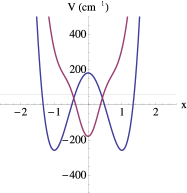
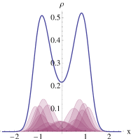
Figure 1: (a) Model double well potential(blue) and partner potential (purple). The energies of the tunneling doublets are indicated by the horizontal lines at $V=0\,{\rm cm}^{-1}$ and $V=59.32\,{\rm cm}^{-1}$ indicating the positions of the sub-barrier tunneling doublet. (b) Final ground state density (blue) superimposed over the Gaussians used in its expansion. (purple)

For a computational example, we take the double well potential to be of the form

$$V_{1}(x)=ax^{4}+bx^{2}+E_{o}.$$ (25)

with $a=438.9{\rm cm}^{-1}/(bohr^{2})$, $b=877.8{\rm cm}^{-1}/(bohr)^{4}$, and $E_{o}=-181.1{\rm cm}^{-1}$ which (for $m=m_{H}$ ) gives rise to exactly two states at below the barrier separating the two minima with a tunneling splitting of 59.32 ${\rm cm}^{-1}$ as computed using a discrete variable representation (DVR) approach.Light et al. (1985) For the calculations reported here, we used $n_{p}=1000$ sample points and $N=15$ Gaussians and in the expansion of $\rho_{T}(x)$ to converge the ground state. This converged the ground state to $1:10^{-8}$ in terms of the energy. This, in itself is encouraging since the accuracy of typical Monte Carlo evaluation would be $1/\sqrt{n_{p}}\approx 3\%$ in terms of the energy. Plots of $V_{1}$ and the converged ground state is shown in Fig. 1.

The partner potential $V_{2}=W^{2}+\hbar W^{\prime}/\sqrt{2m}$, can be constructed once we know the superpotential, $W(x)$. Here, we require an accurate evaluation of the ground state density and its first two log-derivatives. The advantage of our computational scheme is that one can evaluate these analytically for a given set of coefficients. In Fig. 1a we show the partner potential derived from the ground-state density. Where as the original $V_{1}$ potential exhibits the double well structure with minima near $x_{o}=\pm 1$ , the $V_{2}$ partner potential has a pronounced dip about $x=0$. Consequently, its ground-state should have a simple “gaussian”-like form peaked about the origin.

Once we determined an accurate representation of the partner potential, it is now a trivial matter to re-introduce the partner potential into the optimization routes. The ground state converges easily and is shown in Fig. 2a along with its gaussians. After 1000 CG steps, the converged energy is within 0.1% of the exact tunneling splitting for this model system. Again, this is an order of magnitude better than the $1/\sqrt{n_{p}}$ error associated with a simple Monte Carlo sampling. Furthermore, Fig. 2b shows $\psi_{1}^{(1)}\propto A^{\dagger}\psi_{0}^{(2)}$ computed using the converged $\rho_{0}^{(2)}$ density. As anticipated, it shows the proper symmetry and nodal position.

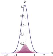
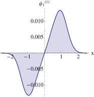
Figure 2: (a) Ground state density of the partner Hamiltonian $H_{2}$ (blue) superimposed over its individual Gaussian components. (b) Excited state $\psi_{1}^{(1)}$ derived from the ground state of the partner potential, $\psi_{o}^{(2)}$.

By symmetry, one expects the node to lie precisely at the origin. However, since we have not imposed any symmetry restriction or bias on our numerical method, the position of the node provides a sensitive test of the convergence of the trial density for $\rho_{0}^{(2)}$. In the example shown in Fig.3, the location of the node oscillates about the origin and appears to converge exponentially with number of CG steps. This is remarkably good considering that this is ultimately determined by the quality of the 3rd and 4th derivatives of $\rho_{o}^{(1)}$ since these appear when computing the conjugate gradient of $V_{2}$. We have tested this approach on a number of other one-dimensional bound-state problems with similar success.

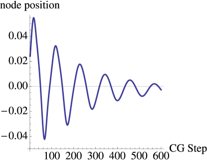
Figure 3: Location of excited state node for the last 600 CG steps.

V Extension to higher dimensions

Having demonstrated that the SUSY approach can be used to compute excitation energies and wave functions starting from a Monte Carlo approach, the immediate next step is to extend this to arbitrarily higher dimensions. To move beyond one dimensional SUSY, Ioffe and coworkers have explored the use of higher-order charge operators A.A.Andrianov et al. (1993); Andrianov et al. (1995); Cannata et al. (2002); Andrianov et al. (2002), and Kravchenko has explored the use of Clifford algebrasKravchenko (2005). Unfortunately, this is difficult to do in general. The reason being that the Riccati factorization of the one-dimensional Schrödinger equation does not extend easily to higher dimensions. One remedy is write the charge operators as vectors $\vec{q}=(+\vec{\partial}+\vec{W})$ and with $\vec{q}^{+}=(-\vec{\partial}+\vec{W})^{T}$ as the adjoint charge operator. The original Schrödinger operator is then constructed as an inner-product

$$H_{1}=\vec{q}^{+}\cdot\vec{q}.$$ (26)

Working through the vector product produces the Schrödinger equation

$$H_{1}\phi=(-\nabla^{2}+W^{2}-(\vec{\nabla}\cdot\vec{W}))\phi=0$$ (27)

and a Riccati equation of the form

$$U(x)=W^{2}-{\rm div}\vec{W}.$$ (28)

For a 2d harmonic oscillator, we would obtain a vector superpotential of the form

$$\vec{W}=-\frac{1}{\psi_{0}^{(1)}}{\rm grad}\psi_{0}^{(1)}=\left(x,y\right)=(W_{x},W_{y})$$ (29)

Let us look at the ${\rm div}\vec{W}$ part closer: If we us the form that $\vec{W}=-\vec{\nabla}\ln\psi$, then $-\vec{\nabla}\cdot\vec{\nabla}\ln\psi=-\nabla^{2}\ln\psi$ which for the 2D oscillator results in ${\rm div}\vec{W}=2$. Thus,

$$W^{2}-{\rm div}\vec{W}=(x^{2}+y^{2})-2$$ (30)

which agrees with the original symmetric harmonic potential. Now, we write the scaled partner potential as

$$U_{2}=W^{2}+{\rm div}\vec{W}=(x^{2}+y^{2})+2.$$ (31)

This is equivalent to the original potential shifted by a constant amount.

$$U_{2}=U_{1}+4.$$ (32)

The ground state in this potential would be have the same energy as the states of the original potential with quantum numbers $n+m=2$. Consequently, even with the this naïve factorization, one can in principle obtain excitation energies for higher dimensional systems, but there is no assurance that one can reproduce the entire spectrum of states.

The problem is neither Hamiltonian $H_{2}$ nor its associated potential $U_{2}$ is given correctly by the form implied by Eq. 27 and Eq. 31. Rather, the correct approach is to write the $H_{2}$ Hamiltonian as a tensor by taking the outer product of the charges $\overline{H}_{2}=\vec{q}\vec{q}^{+}$ rather than as a scaler $\vec{q}\cdot\vec{q}^{+}$. At first this seems unwieldy and unlikely to lead anywhere since the wave function solutions in the second sector are now vectors rather than scalers. However, rather than adding an undue complexity to the problem, it actually simplifies matters considerably. As we demonstrate in a forthcoming paper, this tensor factorization preserves the SUSY algebraic structure and produces excitation energies for any dimensional SUSY system. Moreover, this produces a scaler$\mapsto$ tensor $\mapsto$ scaler hierarchy as one moves to higher excitations.Kouri and Bittner

VI Discussion

In brief, we have used the ideas of SUSY quantum mechanics to obtain excitation energies and excited state wavefunctions within the context of a Monte Carlo scheme. This was accomplished without pre-specifying the location of nodes or restriction to a specific symmetry. While it is clear that one could continue to determine the complete spectrum of $H_{1}$, the real challenge is to extend this technique to higher dimensions. Furthermore, the extension to multi-Fermion systems may be accomplished through the use of the Gaussian Monte Carlo method in which any quantum state can be expressed as a real probability distribution. Corney and Drummond (2004); Assaad et al. (2005) We offer this paper as the starting point for stimulating interest in developing numerical techniques based upon SUSY quantum mechanics.