Medium-modified DGLAP evolution of fragmentation functions from large to small $\boldsymbol{x}$

S. Albino, B.A. Kniehl & R. Pérez-Ramos

II. Institut für Theoretische Physik, Universität Hamburg
Luruper Chaussee 149, D-22761 Hamburg, Germany

Abstract: The unified description of fragmentation function evolution from large to small $x$ which was developed for the vacuum in previous publications is now generalized to the medium, and is studied for the case in which the complete contribution from the largest class of soft gluon logarithms, the double logarithms, are accounted for and with the fixed order part calculated to leading order. In this approach it proves possible to choose the remaining degrees of freedom related to the medium such that the distribution of produced hadrons is suppressed at large momenta while the production of soft radiation-induced charged hadrons at small momenta is enhanced, in agreement with experiment. Just as for the vacuum, our approach does not require further assumptions concerning fragmentation and is more complete than previous computations of evolution in the medium.

Keywords: Perturbative quantum chromodynamics; DGLAP evolution; fragmentation functions; quark-gluon plasma

1 Introduction

The current description of the inclusive production of single hadrons in $e^{+}e^{-}$, $ep$ and hadron collision experiments is provided by the parton model of perturbative QCD (pQCD) involving vacuum fragmentation functions (FFs) $D_{a}^{h}(x,Q^{2})$ ($D$ is a vector containing all quark FFs $D_{q}$, all antiquark FFs $D_{\bar{q}}$ and the gluon FF $D_{g}$), each of which corresponds at lowest order to the probability for a parton $a$ produced in the vacuum at short distance $1/Q$ to form a jet that includes the hadron $h$ carrying a fraction $x$ of the longitudinal momentum of $a$. Different theoretical approximations to the $Q^{2}$ evolution have been derived depending on the kinematical region of $x$: fixed order (FO) calculations at intermediate and large $x$ and resummation to all orders of soft gluon logarithms (SGLs) at small $x$. In Ref. [1], an approach which unifies the double logarithmic approximation (DLA) at small $x$ and the leading order (LO) Dokshitzer-Gribov-Lipatov-Altarelli-Parisi (DGLAP) [2] evolution of FFs at large $x$ was introduced. This approach resums both SGLs and FO logarithms in a consistent way and is defined to any order, and thus allows for a determination of quark and gluon FFs over a wider range of the data than previously achieved. It was shown to describe well both the general features of the “hump-backed plateau” [3] at small $x$, without affecting the quality of the excellent FO description of the large-$x$ region.

In this paper we are concerned with the more general case of medium-modified FFs in heavy-ion collision experiments at all possible values of $x$. In contrast to fragmentation in a vacuum, the fragmenting partons in these reactions are believed to first propagate through a quark-gluon plasma (QGP), which affects the FF evolution. Indeed, recent experiments at the BNL Relativistic Heavy Ion Collider (RHIC) have revealed the phenomenon of a strong suppression of hadrons at high transverse momentum [4, 5], in contrast to the expectations of the parton model and the observations from proton-(anti)proton collisions, which supports the picture that hard partons going through dense matter suffer a significant energy loss prior to hadronization in the vacuum (for a recent review see Ref. [6]). Thus the study of medium-modified FFs may lead to a better understanding of the physical origin of the energy loss effect by serving as a QGP thermometer in the nuclear matter [7]. The study of parton energy loss and medium-modified observables would ideally require the re-construction of jets in heavy-ion collisions. Of course, the huge background makes this task highly delicate. Nevertheless, thanks in particular to important theoretical developments on the jet re-construction algorithms [8] in a high-multiplicity environment, future analyses at the LHC by ALICE [9] and CMS [10] look very promising.

Predictions for multiparticle production in such reactions at small $x$ can be carried out by using a QCD-inspired model for the effect of the medium on the single particle inclusive distribution inside high energy jets [3], the so-called “distorted hump-backed plateau”. For example, such a model was applied in Ref. [11] in the framework of the modified leading logarithmic approximation (MLLA) . In this model, soft emissions, which manifest themselves in the DGLAP splitting functions [2] at small $x$ as SGLs in general and as $1/x$ infra-red singularities at LO, are enhanced at LO by multiplication of a nuclear medium factor $N_{s}>1$. This enhancement can be interpreted as the phenomenological description of the experimentally observed softening of jet spectra in nucleus-nucleus collisions. From the theoretical point of view, the enhancement can be seen as arising from some effective lagrangian which would be suitable for processes in a dense nuclear environment.

If $x$ is too small, the $1/x$ rise of the LO splitting functions is not physically correct since the FO approach becomes invalid. In physical applications, the effect of the enhancement on the complete resummed contribution of double logarithms (DLs) to all orders, of which the $1/x$ term is only the LO contribution, must be calculated by applying this enhancement to an evolution equation suitable for small $x$, such as the double logarithm approximation (DLA) that follows from angular ordering (AO) [3], or the MLLA master equation as was done in Ref. [11].

In this paper, we extend the approach of Ref. [1] to the medium in order to have a formalism which is suitable from large- to small-$x$ values. This approach in the vacuum is more complete than the MLLA since it also incorporates the FO part of the splitting functions, which are important for describing the evolution at large $x$, and thus is more suitable for global fits. In particular, this approach allows for the use of small-$x$ data to add further constraints on FFs at large $x$ to those already provided by large-$x$ data. To apply this approach to the medium involves simply repeating the same steps but in the context of the medium: we resum the medium-modified DLs, being the largest SGLs, in the standard DGLAP evolution by using the medium-modified DLA, in order to improve the small-$x$ description of medium-modified evolution, while the effect of the medium on the FO part is imposed to ensure the correct description at large $x$. Just as for the vacuum, this approach can be extended to higher orders in the FO part and to higher classes of SGLs. Note that we do not impose momentum conservation, since partons can lose energy into the medium, which acts on the fragmenting partons as an external colour field.

The rest of the paper is organized as follows. In section 2, we discuss the modifications to the FO splitting functions due to medium effects. Using these results, we resum the DLs in section 3 using the DLA equation to obtain a DGLAP evolution valid from large to small $x$. Finally, in section 4 we present our conclusions. The medium-modified form of the MLLA is derived in appendix A.

2 Medium-modified fixed order DGLAP evolution equations

In both the vacuum and the medium, the DGLAP evolution takes the form

$$\frac{d}{d\ln Q^{2}}D(x,Q^{2})=\int_{x}^{1}\frac{dz}{z}P(z,a_{s}(Q^{2}))D\left(\frac{x}{z},Q^{2}\right),$$ (1)

where $P$ is the matrix of splitting functions. At large $x$, it is accurately calculated from the FO approach in perturbation theory, which yields a truncation of the series

$$P(x,a_{s})=\sum_{n=1}^{\infty}a_{s}^{n}P^{(n-1)}(x)$$ (2)

at some order in $a_{s}=\alpha_{s}/(2\pi)$, which has the LO $Q^{2}$ evolution $a_{s}(Q^{2})=1/(\beta_{0}\ln(Q^{2}/\Lambda_{QCD}^{2}))$, where $\beta_{0}=(11/6)C_{A}-(2/3)T_{R}n_{f}$ is the first coefficient of the beta function and $\Lambda_{QCD}$ is the asymptotic scale parameter of QCD. In Mellin space, defined as the integral transformation

$$F(\omega)=\int_{0}^{1}dx\,x^{\omega}F(x)$$ (3)

for any function $F(x)$, the convolution in Eq. (1) becomes the simple product

$$\frac{d}{d\ln Q^{2}}D(\omega,Q^{2})=P(\omega,a_{s}(Q^{2}))D(\omega,Q^{2}).$$ (4)

The Mellin transform is invertible, with the inversion given by

$$F(x)=\frac{1}{2\pi i}\int_{C}d\omega\,x^{-\omega-1}F(\omega),$$ (5)

where the integration contour $C$ in the complex $\omega$ plane is parallel to the imaginary axis and to the right of all singularities of the integrand $F(\omega)$. By using charge conjugation and SU($n_{f}$) flavour symmetry to decompose the DGLAP equation into 3 simpler types of equations, Eq. (4) can be solved analytically up to the desired order in $a_{s}$, making the calculation of evolved FFs via the inverse Mellin transform numerically more efficient than the direct integration of Eq. (1). These 3 types of equations are the DGLAP equations for the non-singlet and valence quark FFs in which $P$ is a 1$\times$1 matrix, and the DGLAP equation for $D=(D_{\Sigma},D_{g})$, where $P(x,a_{s})$ is the 2$\times$2 matrix which we write as

$$P=\left(\begin{array}[]{cc}P_{\Sigma\Sigma}&P_{\Sigma g}\\ P_{g\Sigma}&P_{gg}\end{array}\right).$$ (8)

We begin with a study of the medium modifications to the latter DGLAP equation. After multiple rescattering in a dense nuclear medium, a relativistic parton loses a significant fraction of its energy scale. In the soft multiple momentum transfer model of the medium [12], the singular terms $\propto 1/x$ (as $x\to 0$) and, by the LO symmetry of the parton splitting process for all $x\neq 1$ under $x\rightarrow 1-x$, also the singular terms $\propto 1/(1-x)$ (as $x\to 1$) are simply multiplied by a nuclear factor $N_{s}$ [11] such that soft emission is enhanced. Applying these modifications to the LO splitting functions in the vacuum [3, 2], the LO splitting functions in the medium using the notation of Eq. (2) become

$$P_{\Sigma g}^{(0)}(x)\!\! \!\!=\!\! \!\!4C_{F}\left(\frac{N_{s}}{x}+f_{\Sigma g}(x)\right),\quad P_{\Sigma\Sigma}^{(0)}(x)=2C_{F}\left(\left[\frac{N_{s}}{1-x}\right]_{+}+f_{\Sigma\Sigma}(x)\right),$$ (9)

$$P_{gg}^{(0)}(x)\!\! \!\!=\!\! \!\!2C_{A}\left(\frac{N_{s}}{x}+\left[\frac{N_{s}}{1-x}\right]_{+}+f_{gg}(x)\right),\quad P_{g\Sigma}^{(0)}(x)=n_{f}T_{R}f_{g\Sigma}(x),$$ (10)

where $C_{F}$ and $C_{A}$ are respectively the casimirs of the fundamental and adjoint representations of the QCD color gauge group $SU(3)_{c}$, $T_{R}=1/2$ and $n_{f}$ is the number of active (anti)quark flavours. The plus distribution applied to a function $F(x)$, written $[F(x)]_{+}$, is defined by

$$\int_{0}^{1}dx[F(x)]_{+}g(x)=\int_{0}^{1}dxF(x)\left[g(x)-g(1)\right]$$ (11)

for any function $g(x)$. The functions $f_{ab}(x)$ are regular in the limit $x\to 0$. In particular, the Borghini-Wiedemann choice [11] is recovered by choosing the $f_{ab}(x)$ to be equal to their vacuum forms $\left[f_{ab}(x)\right]_{N_{s}=1}$ given for $x\neq 1$ by

$$\left[f_{\Sigma g}(x)\right]_{N_{s}=1}\!\! \!\!=\!\! \!\!\frac{x}{2}-1,\quad\left[f_{\Sigma\Sigma}(x)\right]_{N_{s}=1}=-\frac{x}{2}-\frac{1}{2},$$ (12a)

$$\left[f_{gg}(x)\right]_{N_{s}=1}\!\! \!\!=\!\! \!\!x(1-x)-2,\quad\left[f_{g\Sigma}(x)\right]_{N_{s}=1}=x^{2}+(1-x)^{2}.$$ (12b)

(The delta functions at $x=1$ along the diagonal of the splitting functions can be determined by momentum conservation.)

However, the correct model for the medium is not known at present, therefore neither the value of $N_{s}$ nor the $f_{ab}(x)$ are known. We note that a more complete form for the medium-modified splitting functions $P(x,a_{s})$ may be derived from some effective lagrangian ${\cal L}_{med}\propto(F^{c}_{\mu\nu,med})^{2}$ in the medium.

The DGLAP evolution of the non-singlet and valence quark FFs is accurately described for large- to small-$x$ values when the splitting function is calculated in the FO approach, since it is free of SGLs to all orders. Furthermore, the splitting function behaves like $\sim 1/(1-x)$ to all orders. Therefore, the effect of the medium on the large-$x$ LO evolution of these FFs is incorporated simply by multiplying the $1/(1-x)$ singularities in the non-singlet and valence quark splitting functions by $N_{s}$, and replacing the rest of these functions by an unknown function which is non singular as $x\rightarrow 0,1$ (apart from possible delta functions at $x=1$).

In Mellin space,

$$P_{\Sigma g}^{(0)}(\omega)\!\! \!\!=\!\! \!\!4C_{F}\left(\frac{N_{s}}{\omega}+f_{\Sigma g}(\omega)\right),$$ (13)

$$P_{\Sigma\Sigma}^{(0)}(\omega)\!\! \!\!=\!\! \!\!2C_{F}\left(-N_{s}S_{1}(\omega)+f_{\Sigma\Sigma}(\omega)\right),$$ (14)

$$P_{gg}^{(0)}(\omega)\!\! \!\!=\!\! \!\!2C_{A}\left(\frac{N_{s}}{\omega}-N_{s}S_{1}(\omega)+f_{gg}(\omega)\right),$$ (15)

$$P_{g\Sigma}^{(0)}(\omega)\!\! \!\!=\!\! \!\!n_{f}T_{R}f_{g\Sigma}(\omega),$$ (16)

where the harmonic sum $S_{1}(\omega)=\sum_{n=1}^{\omega}1/n$ for integer $\omega$. The Mellin transform of the small-$x$ singularity $1/x$ is proportional to the small-$\omega$ singularity $1/\omega$ (note $S_{1}(0)=0$), while the Mellin transform of the large-$x$ singularity $1/(1-x)$ grows at large $|\omega|$ as $\ln\omega$ (because $S_{1}(\omega)\simeq\ln\omega$ here). Because $P_{\Sigma g}^{(0)}(\omega)$ and $P_{g\Sigma}^{(0)}(\omega)$ remain finite as $|\omega|$ approaches infinity, while

$$P_{aa}^{(0)}(\omega)\approx-2C_{a}N_{s}\ln\omega,\qquad\omega\gg 1,$$ (17)

where

$$C_{\Sigma}=C_{F},\,\,C_{g}=C_{A},$$ (18)

one finds, after using Eqs. (4) and (5), the following behavior of the quark singlet and gluon FFs at large $Q$:

$$D_{a}(x,Q^{2})\sim(1-x)^{-1+4C_{a}N_{s}\Delta\xi(a_{s}(Q^{2}))},\quad\Delta\xi(a_{s})=\frac{1}{2\beta_{0}}\ln a_{s}.$$ (19)

The non-singlet and valence quark FFs will exhibit the same behaviour with $C_{a}=C_{F}$. Therefore, FFs at large $x$ decrease when $N_{s}$ increases (provided that the exponent in Eq. (19) is positive, which is the case at large $Q$). Consequently, the production of hard hadrons gets restricted at large $x$ or, equivalently, in the large-$p_{T}$ region in particle production in heavy-ion collisions.

The small-$x$ behavior of FFs is controlled by the behavior of the splitting functions in Mellin space near $\omega=0$. In the next section we will show that, in this region, the approximate behavior of $D_{a}(x,Q^{2})$ as a function of $\ell=\ln(1/x)$ is given by

$$xD_{a}(x,Q^{2})\sim{\cal N}\exp\left[-\frac{1}{2\sigma^{2}}(\ell-\bar{\ell})^{2}\right],$$ (20)

where the average multiplicity increase is given by [13]

$${\cal N}\sim\exp\left(\frac{1}{\beta_{0}}\sqrt{\frac{4N_{s}C_{A}}{a_{s}(Q^{2})}}\right).$$ (21)

Hence the production of soft hadrons gets enhanced in the medium at small $x$.

3 Evolution equations from large to small $\boldsymbol{x}$

In the medium, the DLA-improved evolution equation for $D=(D_{\Sigma},D_{g})$, which was introduced for the vacuum in Ref. [1] and which is valid from large to small $x$, becomes

$$\frac{d}{d\ln Q^{2}}D(z,Q^{2})\!\! \!\!=\!\! \!\!\int_{z}^{1}\frac{dz^{\prime}}{z^{\prime}}\frac{2C_{A}N_{s}}{z^{\prime}}Az^{{}^{\prime}2\frac{d}{d\ln Q^{2}}}\left[a_{s}(Q^{2})D\left(\frac{z}{z^{\prime}},Q^{2}\right)\right]$$ (22)

$$\!\!+\!\! \!\!\int_{z}^{1}\frac{dz^{\prime}}{z^{\prime}}\bar{P}(z^{\prime},a_{s}(Q^{2}))D\left(\frac{z}{z^{\prime}},Q^{2}\right).$$

where the matrix $A$ is given by

$${A}=\left(\begin{array}[]{cc}0&\frac{2C_{F}}{C_{A}}\cr 0&1\end{array}\right).$$

Equation (22) is obtained by multiplying by $N_{s}$ the $1/x$ factor in the first term on the right hand side. At LO, the $1/(1-x)$ singularities in the function $\bar{P}$ must be similarly enhanced, as dictated by the soft multiple momentum transfer model of the medium. Setting $N_{s}=1$ in Eq. (22), we recover the DLA-improved vacuum evolution equation of Ref. [1]. Since $\bar{P}$ is free of DLs to all orders, Eq. (22) can be used to determine the complete DL contribution to $P$. We note that $\bar{P}$ contains other SGLs beyond LO, which are less significant than DLs but significant nonetheless, and the effect of the medium on these SGLs is not known.

By using the approach of Ref. [1], we will use Eq. (22) to obtain an evolution which is valid to DL accuracy at small $x$ and to LO accuracy at large $x$. This goal can be achieved by repeating precisely the steps of Ref. [1], which we briefly outline here: We use Eq. (3) to put Eq. (22) in Mellin space,

$$\left(\omega+2\frac{d}{d\ln Q^{2}}\right)\frac{d}{d\ln Q^{2}}D=2C_{A}N_{s}a_{s}AD+\left(\omega+2\frac{d}{d\ln Q^{2}}\right)\bar{P}D,$$ (23)

where we have set $D=D(\omega,Q^{2})$, $a_{s}=a_{s}(Q^{2})$ and $\bar{P}=\bar{P}(\omega,a_{s})$ for brevity. Substituting Eq. (4) into Eq. (23) and setting

$$P=P^{\rm DL}+P^{\line(2,1){12.5}{\rm DL}},$$ (24)

where $P^{\rm DL}$ represents the complete DL contribution to $P$ and the remainder $P^{\line(2,1){12.5}{\rm DL}}$ everything else, and then taking the leading term (see Refs. [1, 14] for a more detailed discussion), one gets the equation

$$2\left(P^{\text{DL}}\right)^{2}+\omega P^{\text{DL}}-2C_{A}N_{s}a_{s}A=0,$$ (25)

whose only solution consistent with perturbation theory is [1]

$$P^{\text{DL}}(\omega,a_{s})=\frac{A}{4}\left(-\omega+\sqrt{\omega^{2}+16C_{A}N_{s}a_{s}}\right),$$ (26)

which is the Mellin transform of

$$P^{\text{DL}}(x,a_{s})=\frac{A\sqrt{C_{A}N_{s}a_{s}}}{x\ln\frac{1}{x}}J_{1}\left(4\sqrt{C_{A}N_{s}a_{s}}\ln\frac{1}{x}\right),$$ (27)

where $J_{1}$ is the Bessel function of the first kind.

Our unified approach to medium-modified evolution in the case of DL accuracy at small $x$ and LO accuracy at large $x$ can now be formulated, as follows: The evolution is performed using Eq. (1) with $P$ approximated as in Eq. (24), where $P^{\rm DL}$ is given by Eq. (27) and $P^{\line(2,1){12.5}{\rm DL}}$ is set equal to the LO splitting function after its DLs have been subtracted to prevent double counting, viz.

$$P(\omega,a_{s})=P^{\rm DL}(\omega,a_{s})+a_{s}P^{\line(2,1){12.5}{\rm DL}(0)}(\omega),$$ (28)

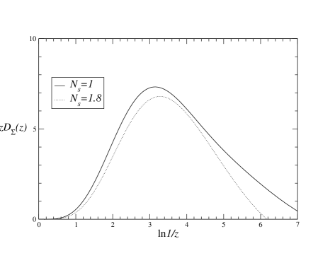
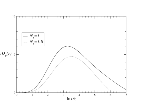
Figure 1: Quark singlet (left) and gluon (right) FFs evolved in the vacuum ($N_{s}=1$) and in the medium ($N_{s}=1.8$) from a factorization scale $Q=10$ to $100$ GeV and with the choice $f_{ab}=N_{s}\left[f_{ab}\right]_{N_{s}=1}$. At the initial scale, the choice $D_{g}=(C_{A}/(2C_{F}))D_{\Sigma}=N\exp[-c\ln^{2}z]x^{\alpha}(1-x)^{\beta}$ is made where, motivated by the results of Ref. [1], we have taken $N=1.6$, $c=0.35$, $\alpha=-2.63$ and $\beta=3$.

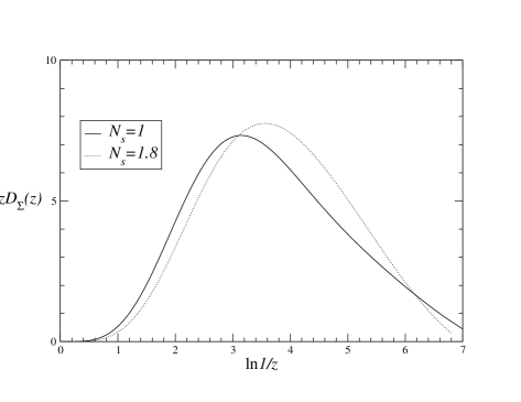
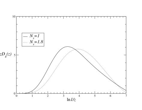
Figure 2: As in Fig. 1, but with $f_{ab}=\left[f_{ab}\right]_{N_{s}=1}$.

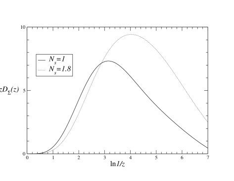
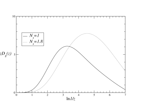
Figure 3: As in Fig. 1, but with $f_{ab}=0$.

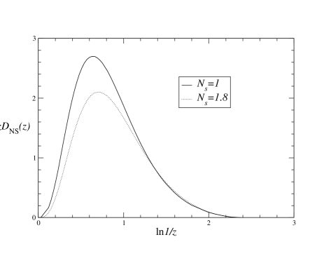
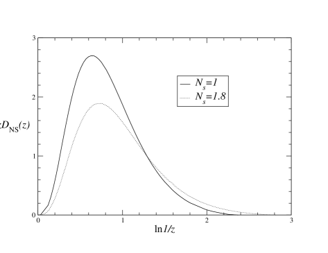
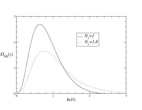
Figure 4: As in Figs. 1 (top left), 2 (top right) and 3 (bottom), but for the non-singlet quark FF with $N=500$, $c=0$, $\alpha=3$ and $\beta=3$.

where $a_{s}P^{\line(2,1){12.5}{\rm DL}(0)}(0)$ is the LO term in the expansion of $P^{\line(2,1){12.5}{\rm DL}}(\omega,a_{s})$ in $a_{s}$. Higher order terms in $P^{\line(2,1){12.5}{\rm DL}}(\omega,a_{s})$ may also be included, provided the SGLs contained within them are subtracted [1] (or resummed, which is not possible at present). In other words, the splitting functions in Mellin space are given by

$$P_{\Sigma g}^{(0)}(\omega)\!\! \!\!=\!\! \!\!\frac{C_{F}}{2C_{A}}\left(-\omega+\sqrt{\omega^{2}+16C_{A}N_{s}a_{s}}\right)+4C_{F}f_{\Sigma g}(\omega),$$

$$P_{\Sigma\Sigma}^{(0)}(\omega)\!\! \!\!=\!\! \!\!-2C_{F}N_{s}S_{1}(\omega)+2C_{F}f_{\Sigma\Sigma}(\omega),$$

$$P_{gg}^{(0)}(\omega)\!\! \!\!=\!\! \!\!\frac{1}{4}\left(-\omega+\sqrt{\omega^{2}+16C_{A}N_{s}a_{s}}\right)-2C_{A}N_{s}S_{1}(\omega)+2C_{A}f_{gg}(\omega),$$

$$P_{g\Sigma}^{(0)}(\omega)\!\! \!\!=\!\! \!\!n_{f}T_{R}f_{g\Sigma}(\omega).$$ (29)

The results in Eq. (3) are the main results of this paper.

In order to understand better the $f_{ab}$, we plot the evolved FFs in the vacuum and in the medium for different choices of them to see which give the most physically expected results, namely an enhancement of hadron production at small $x$ due to induced soft gluon radiation by the medium, and a suppression of this production at large $x$ due to parton energy loss in the medium. We choose a fragmentation scale of 100 GeV which is suitable for the LHC. To account for medium effects, we adopt the value $N_{s}=1.8$ from Ref. [11]. We choose the vacuum and medium FFs to be equal at 10 GeV, which is consistent with a finite-sized medium. In Fig. 1, we choose $f_{ab}=N_{s}\left[f_{ab}\right]_{N_{s}=1}$ for the evolution in the medium (we absorb the delta functions at $x=1$ into the definition of the $f_{ab}$ here and in what follows), i.e. the magnitudes of the $f_{ab}$ are chosen to be greater than their vacuum values. In Fig. 2, we choose the vacuum values exactly, $f_{ab}=\left[f_{ab}\right]_{N_{s}=1}$, while in Fig. 3 we set $f_{ab}=0$. Therefore, physically expected results can be obtained when the $f_{ab}$ are chosen to not increase with $N_{s}$. Note that for all choices of the $f_{ab}$ there is always a suppression at large $x$.

Finally, we show the non-singlet (or valence) quark evolution in Fig. 4. Such an FF gives a measure of the excess of e.g. charged over neutral kaon production [15], or of positively charged over negatively charged hadrons. In this case there are no soft gluon logarithms at small $x$, and therefore there is no Gaussian behaviour at small $x$, but rather an $x^{\alpha}$ behaviour, and the FO approach for the evolution is expected to be reliable from the largest- to smallest-$x$ values. Just as for the quark singlet and gluon FFs, we find that the medium induces a suppression at large $x$ and an enhancement at small $x$ provided that the $f_{ab}$ do not increase with $N_{s}$.

3.1 Small-$\boldsymbol{x}$ limit

We now derive the small-$x$ behaviour given by Eqs. (20) and (21). The medium modifications to the MLLA will be derived in appendix A as an extension to the results below. In the small-$x$ region we may neglect the second term in Eq. (28), i.e. we may take

$$P(\omega,a_{s})=P^{\rm DL}(\omega,a_{s}).$$ (30)

Then the solution to the gluon component of Eq. (43) reduces to the simple form

$$D_{g}(\omega,Q^{2})=E_{gg}(\omega,a_{s}(Q^{2}),a_{s}(Q_{0}^{2}))D_{g}(\omega,Q_{0}^{2})$$ (31)

with

$$E_{gg}(\omega,a_{s}(Q^{2}),a_{s}(Q_{0}^{2}))=\exp\left[\int_{Q_{0}}^{Q}d\ln Q^{\prime 2}P_{gg}(\omega,a_{s}(Q^{\prime 2}))\right],$$ (32)

where

$$P_{gg}(\omega,a_{s})\!\! \!\!=\!\! \!\!\frac{1}{4}\left(-\omega+\sqrt{\omega^{2}+16C_{A}N_{s}a_{s}}\right).$$ (33)

At small $x$, one can predict the shape and normalization of the medium-modified FFs using the same procedure as for the vacuum FFs in Ref. [16], where the expression for $\left[D_{a}(x,Q^{2})\right]_{N_{s}=1}$ was derived by writing the solution in the form of a distorted Gaussian,

$$xD_{g}(x,Q^{2})=\frac{{\cal N}}{\sigma\sqrt{2\pi}}\exp\left[\frac{1}{8}k-\frac{1}{2}s\delta-\frac{1}{4}(2+k)\delta^{2}+\frac{1}{6}s\delta^{3}+\frac{1}{24}k\delta^{4}\right].$$ (34)

In this expression, $\delta=(\ell-\bar{\ell})/\sigma$, ${\cal N}$ is the asymptotic average multiplicity inside a gluon jet (Eq. (21)), $\bar{l}$, $\sigma$, $s$ and $k$ are respectively the position of the peak, the dispersion, the skewness and the kurtosis of the distribution. They are given by

$$\bar{\ell} = K_{1},$$

$$\sigma = \sqrt{K_{2}},$$

$$s = \frac{K_{3}}{\sigma^{3}},$$

$$k = \frac{K_{4}}{\sigma^{4}},$$ (35)

where $K_{n}$ is the $n$th moment of $D_{g}$:

$$K_{n}(Q^{2})=\left(-\frac{d}{d\omega}\right)^{n}\ln[D_{g}(\omega,Q^{2})]_{\omega=0}.$$

The reason why Eq. (34) is valid around the position of the peak (i.e. for $\delta=O(1)$) is because the exponent is believed to be an expansion in $a_{s}$, and this is the case in the MLLA. We now determine the distorted Gaussian parameters as a function of $a_{s}$ and also $N_{s}$. The extension to the MLLA is given in appendix A. According to Eq. (31), the $K_{n}(Q^{2})$ evolve as

$$K_{n}(Q^{2})=\Delta K_{n}(a_{s}(Q^{2}),a_{s}(Q_{0}^{2}))+K_{n}(Q_{0}^{2}),$$ (36)

where $\Delta K_{n}(a_{s}(Q^{2}),a_{s}(Q_{0}^{2}))$ is the $n$th moment of $E_{gg}(\omega,a_{s}(Q^{2}),a_{s}(Q_{0}^{2}))$, given by

$$\Delta K_{n}(a_{s}(Q^{2}),a_{s}(Q_{0}^{2}))=\int_{Q_{0}}^{Q}d\ln Q^{\prime 2}\left(-\frac{d}{d\omega}\right)^{n}P_{gg}(\omega,a_{s}(Q^{\prime 2})).$$

We now make the approximation that any constants and $Q_{0}$-dependent terms in Eq. (36) can be neglected, which is valid for sufficiently large $Q$. Making use of Eq. (33), one finds

$$K_{1} = \frac{a_{s}^{-1}}{4\beta_{0}},$$

$$K_{2} = \frac{a_{s}^{-3/2}}{6\beta_{0}\sqrt{16C_{A}N_{s}}},$$

$$K_{3} = 0,$$

$$K_{4} = -\frac{3a_{s}^{-5/2}}{10\beta_{0}(16C_{A}N_{s})^{3/2}}.$$ (37)

Then from Eqs. (35) and (3.1), one finds

$$\bar{\ell} = \frac{a_{s}^{-1}}{4\beta_{0}},$$ (38a)

$$\sigma = \frac{a_{s}^{-3/4}}{\sqrt{6\beta_{0}}(16C_{A}N_{s})^{1/4}},$$ (38b)

$$s = 0,$$ (38c)

$$k = -\frac{54}{5}\beta_{0}\sqrt{\frac{a_{s}}{16C_{A}N_{s}}}.$$ (38d)

From these results, we find that the distribution around the position of the peak (i.e. $\delta=O(1)$) can be approximated by a distorted Gaussian, namely Eq. (20). The width (Eq. (38b)) and the kurtosis (Eq. (38d)) of this distorted Gaussian are suppressed in the limit $N_{s}\gg 1$ by $1/N_{s}^{\alpha}$, where $\alpha$ is a positive constant.

Setting $\omega=0$ in Eq. (33), one recovers the rate of the mean average multiplicity increase in a gluon jet with respect to $\ln Q^{2}$, i.e. the DLA medium-modified anomalous dimension of the multiplicity [13]:

$$P_{gg}(0,a_{s})=\sqrt{C_{A}N_{s}a_{s}},$$ (39)

in which case Eqs. (31) and (32) give Eq. (21) at large $Q$.

4 Conclusions

Our approach provides a general framework for the incorporation of medium effects into the DGLAP evolution of FFs from large to small $x$, which will be important for the description of single hadron production in heavy-ion collisions from high to low $p_{T}$. In particular, our approach allows the use of measurements of such observables at low $p_{T}$, e.g. from heavy-ion collisions at the LHC, to provide additional constraints on the medium-modified FFs to those constraints provided by large-$p_{T}$ data, and therefore could improve the ruling out of various models of the medium by improving the constraints on the unknown degrees of freedom.

Appendix A MLLA limit

The MLLA can be regarded as a simplification to the approach of Ref. [1] and of this paper, in which the main qualitative features of hadron production are preserved. We now use our approach to determine the form of the MLLA with medium effects taken into account. The MLLA is obtained by setting $\omega=0$ in the second term in Eq. (28), i.e. by taking

$$P(\omega,a_{s})=P^{\rm DL}(\omega,a_{s})+a_{s}P^{\line(2,1){12.5}{\rm DL}(0)}(0),$$ (40)

which for small $\omega$ is correct to terms of $O(\omega)$. In the case of the medium,

$$P^{\line(2,1){12.5}{\rm DL}(0)}(0)=\left(\begin{array}[]{cc}2C_{F}f_{\Sigma\Sigma}(0)&4C_{F}f_{\Sigma g}(0)\cr n_{f}T_{R}f_{g\Sigma}(0)&2C_{A}f_{gg}(0)\end{array}\right),$$ (41)

which corresponds to the hard SL corrections in the MLLA formalism [3]. Setting

$$D_{\Sigma}=\frac{2C_{F}}{C_{A}}D_{g},$$

the system in Eq. (23) with Eq. (41) reduces to a self-contained equation for $D_{g}$ and a coupled equation for $D_{\Sigma}$, constrained by the solution of $D_{g}$, which can be written in the form

$$\left(\!\!\omega+2\frac{d}{d\ln Q^{2}}\!\!\right)\!\frac{d}{d\ln Q^{2}}D_{\Sigma}\!\! \!\!=\!\! \!\!4C_{F}N_{s}a_{s}D_{g}\!\!+\!\!\left(\!4C_{F}f_{\Sigma g}(0)\!+\!\frac{2C_{F}}{C_{A}}f_{\Sigma\Sigma}(0)\!\right)\!\!\left(\!\!\omega+2\frac{d}{d\ln Q^{2}\!\!}\right)\!\!a_{s}D_{g},$$ (42)

$$\left(\!\!\omega+2\frac{d}{d\ln Q^{2}}\!\!\right)\!\frac{d}{d\ln Q^{2}}D_{g}\!\! \!\!=\!\! \!\!2C_{A}N_{s}a_{s}D_{g}-\frac{1}{2}a_{\text{med}}\left(\!\!\omega+2\frac{d}{d\ln Q^{2}}\!\!\right)a_{s}D_{g}.$$ (43)

In Ref. [11] the choice $N_{s}=1$ is made in $P^{\line(2,1){12.5}{\rm DL}(0)}(0)$, which is known:

$$[P^{\line(2,1){12.5}{\rm DL}(0)}(0)]_{N_{s}=1}=\left(\begin{array}[]{cc}0&-3C_{F}\cr\frac{2}{3}n_{f}T_{R}&-\frac{11}{6}C_{A}-\frac{2}{3}n_{f}T_{R}\end{array}\right),$$ (44)

and in $a_{\text{med}}$, which is also known:

$$[a_{\text{med}}]_{N_{s}=1}=a=\frac{11C_{A}}{3}+\frac{4n_{f}T_{R}}{3}\left(1-\frac{2C_{F}}{C_{A}}\right).$$

However, we will keep $N_{s}\neq 1$ in what follows in order to maintain generality. Using Eqs. (31) and (32), Eq. (43) after some straightforward algebraic operations becomes

$$(\omega+2P_{gg})P_{gg}-2C_{A}N_{s}a_{s}=-2\beta(a_{s})\frac{dP_{gg}}{da_{s}}-\frac{1}{2}a_{\text{med}}(\omega+2P_{gg})a_{s},$$ (45)

which provides the following solution correct to terms of single logarithmic order:

$$P_{gg}(\omega,a_{s})\!\! \!\!=\!\! \!\!\frac{1}{4}\left(-\omega+\sqrt{\omega^{2}+16C_{A}N_{s}a_{s}}\right)$$

$$\!\!+\!\! \!\!a_{s}\left[\beta_{0}\frac{4C_{A}N_{s}a_{s}}{\omega^{2}+16C_{A}N_{s}a_{s}}-\frac{1}{4}a_{\text{med}}\left(1+\frac{\omega}{\sqrt{\omega^{2}+16C_{A}N_{s}a_{s}}}\right)\right].$$

Setting $\omega=0$ in Eq. (A), one recovers the rate of the mean average multiplicity increase in a gluon jet with respect to $\ln Q^{2}$, i.e. the MLLA medium-modified anomalous dimension of the multiplicity [13]:

$$P_{gg}(0,a_{s})=\sqrt{C_{A}N_{s}a_{s}}+\frac{a_{s}}{4}\left(\beta_{0}-a_{\text{med}}\right).$$ (47)

The purpose of $\beta_{0}$ is to account for the running of the coupling constant $a_{s}$. Finally, the solution for $D_{\Sigma}$ at NLO in Mellin space can be derived from Eq. (42), once $D_{g}$ has been computed, and reads

$$D_{\Sigma}=\frac{2C_{F}}{C_{A}}\left\{1+\frac{1}{N_{s}}\left[\frac{1}{4C_{A}}a_{\text{med}}+f_{\Sigma g}(0)+\frac{C_{F}}{C_{A}}f_{\Sigma\Sigma}(0)\right]\left(\omega+2\frac{d}{d\ln Q^{2}}\right)\right\}D_{g}.$$ (48)

Since $\left(\omega+2\frac{d}{d\ln Q^{2}}\right)\simeq{\cal O}(\sqrt{N_{s}a_{s}})$, the second term on the right-hand side of Eq. (48) is of order ${\cal O}(\sqrt{a_{s}/N_{s}})$. For $N_{s}=1$, one recovers the result in the vacuum [17] with

$$\left[\frac{1}{4C_{A}}a_{\text{med}}+f_{\Sigma g}(0)+\frac{C_{F}}{C_{A}}f_{\Sigma\Sigma}(0)\right]_{N_{s}=1}=\frac{a}{4C_{A}}-\frac{3}{4}.$$

Making use of Eq. (A), one finds

$$K_{1} = \frac{a_{s}^{-1}}{4\beta_{0}}+\frac{a_{\text{med}}a_{s}^{-1/2}}{2\beta_{0}\sqrt{16C_{A}N_{s}}},$$

$$K_{2} = \frac{a_{s}^{-3/2}}{6\beta_{0}\sqrt{16C_{A}N_{s}}}-\frac{a_{s}^{-1}}{32C_{A}N_{s}},$$

$$K_{3} = -\frac{a_{\text{med}}a_{s}^{-3/2}}{2\beta_{0}(16C_{A}N_{s})^{3/2}},$$

$$K_{4} = -\frac{3a_{s}^{-5/2}}{10\beta_{0}(16C_{A}N_{s})^{3/2}}+\frac{3a_{s}^{-2}}{(16C_{A}N_{s})^{2}}.$$ (49)

Then from Eqs. (35) and (A), one finds

$${\cal N} = {\cal N}_{0}\exp\left[\frac{2}{\beta_{0}}\sqrt{\frac{C_{A}N_{s}}{a_{s}}}+\frac{1}{4\beta_{0}}\left(a_{\rm med}-\beta_{0}\right)\ln a_{s}\right]$$ (50a)

$$\bar{\ell} = \frac{a_{s}^{-1}}{4\beta_{0}}+\frac{a_{\text{med}}a_{s}^{-1/2}}{2\beta_{0}\sqrt{16C_{A}N_{s}}},$$ (50b)

$$\sigma = \frac{a_{s}^{-3/4}}{\sqrt{6\beta_{0}}(16C_{A}N_{s})^{1/4}}\left(1-\frac{3}{2}\beta_{0}\sqrt{\frac{a_{s}}{16C_{A}N_{s}}}\right),$$ (50c)

$$s = -3\sqrt{6\beta_{0}}\,a_{\text{med}}\left(\frac{a_{s}}{16C_{A}N_{s}}\right)^{3/4},$$ (50d)

$$k = -\frac{54}{5}\beta_{0}\sqrt{\frac{a_{s}}{16C_{A}N_{s}}}\left(1-4\beta_{0}\sqrt{\frac{a_{s}}{16C_{A}N_{s}}}\right),$$ (50e)

which coincide with the results in Ref. [16] in the limit $N_{s}=1$.

Assuming that $a_{\text{med}}$ rises slower than $N_{s}^{3/4}$, the skewness (Eq. (50d)), like the width (Eq. (50c)) and the kurtosis (Eq. (50e)), is suppressed in the limit $N_{s}\gg 1$. As found in subsection 3.1, the distribution close to the position of the peak can be approximated by a Gaussian shape. Finally, in Ref. [11], the choice $\left[a_{\text{med}}\right]_{N_{s}=1}=a$ is made, in which case the position of the peak approaches the asymptotic DLA value $\frac{a_{s}^{-1}}{4\beta_{0}}$ for large $N_{s}$.

References

• [1] S. Albino, B. A. Kniehl, G. Kramer, W. Ochs, Phys. Rev. Lett. 95 (2005) 232002 [hep-ph/0503170]; Phys. Rev. D 73 (2006) 054020 [hep-ph/0510319].
• [2] V. N. Gribov, L. N. Lipatov, Yad. Fiz. 15 (1972) 781 [Sov. J. Nucl. Phys. 15 (1972) 438]; G. Altarelli, G. Parisi, Nucl. Phys. B 126 (1977) 298; Yu. L. Dokshitser, Zh. Eksp. Teor. Fiz. 73 (1977) 1216; [Sov. Phys. JETP 46 (1977) 641].
• [3] Yu. L. Dokshitzer, V. A. Khoze, A. H. Mueller, S. I. Troyan, Basics of Perturbative QCD, Editions Frontières, Paris (1991).
• [4] K. Adcox et al. (PHENIX Collab.), Phys. Rev. Lett. 88 (2002) 022301 [nucl-ex/0109003]; S. S. Adler et al. (PHENIX Collab.), Phys. Rev. Lett. 91 (2003) 072301 [nucl-ex/0304022].
• [5] C. Adler et al. (STAR Collab.), Phys. Rev. Lett. 89 (2002) 202301 [nucl-ex/0206011].
• [6] R. Baier, D. Schiff, B. G. Zakharov, Ann. Rev. Nucl. Part. Sci. 50 (2000) 37 [hep-ph/0002198];
A. Kovner, U. A. Wiedemann, in Quark Gluon Plasma M. Gyulassy, I. Vitev, X.-N. Wang, B.-W. Zhang, nucl-th/0302077;
3, World Scientific, Singapore, hep-ph/0304151;
A. Majumder, J. Phys. G 34 (2007) S377 [nucl-th/0702066];
F. Arleo, hep-ph/08101193;
For a more recent review, see also S. Peigné, A. V. Smilga, hep-ph/08105702.
• [7] N. Armesto, L. Cunqueiro, C. A. Salgado, W. C. Xiang, JHEP 0802 (2008) 048 [arXiv:0710.3073 [hep-ph]].
• [8] M. Cacciari & G. P. Salam, Phys. Lett. B 641 (2006) 57 [hep-ph/0512210].
• [9] ALICE collaboration, B. Alessandro et al., J. Phys. G 32 (2006) 1295.
• [10] CMS collaboration, D. d’Enterria (Ed.) et al., J. Phys. G 34 (2007) 2307.
• [11] N. Borghini, U. A. Wiedemann, hep-ph/0506218; I. M. Dremin, O. S. Shadrin, J. Phys. G 32 (2006) 963; K. Zapp, G. Ingelman, J. Rathsman, J. Stachel, U. A. Wiedemann, arXiv:0804.3568 [hep-ph].
• [12] R. Baier, Y. L. Dokshitzer, A. H. Mueller, S. Peigne, D. Schiff, Nucl. Phys. B 484 (1997) 265 [arXiv:hep-ph/9608322]; C. A. Salgado, U. A. Wiedemann, Phys. Rev. D 68 (2003) 014008 [arXiv:hep-ph/0302184].
• [13] R. Perez-Ramos, arXiv:0811.2418 [hep-ph]; arXiv:0811.2934 [hep-ph].
• [14] S. Albino, arXiv:0810.4255 [hep-ph].
• [15] E. Christova, E. Leader, Phys. Rev. D 79 (2009) 014019 [arXiv:0809.0191 [hep-ph]].
• [16] C. P. Fong, B. R. Webber, Nucl. Phys. B 355 (1991) 54.
• [17] E. D. Malaza, B. R. Webber, Phys. Lett. B 149 (1984) 501; Nucl. Phys. B 267 (1986) 702.