Purity Swapping in the Jaynes-Cummings Model: Obtaining Perfect Interference Patterns from Totally Unpolarized Qubits

Abstract

We show the existence of dynamical purity swapping phenomena in the Jaynes-Cummings model. Moreover we show that purity swapping between a qubit and a generic quantum system is possible, provided they are coupled via non-unitary matrix elements interaction. We particularize to the case of a quantum optical Ramsey interferometer. We show that using purity swapping, a perfect interference pattern can be obtained at the output port of the interferometer even if we start from totally unpolarized sources. This feature is shown to be associated with the phenomena of recreation of the state vector at half of the revival time. In fact, we show that the Gea-Banacloche attractor is robust against degradation of the purity of the qubit input state. We also show that the Tsallis entropy $T_{2}$ is a useful entanglement monotone allowing one to relate directly entanglement with purity exchange in interacting systems. We conjecture an Araki-Lieb type inequality for $T_{2}$ that bounds the maximum interchange of purity between interacting systems.

I Introduction

The Jaynes-Cummings Model (JCM) is a paradigmatic description for many problems involving the interaction of spin-like two-level systems with single mode bosonic systems shore . Examples can be found in a large variety of systems, ranging from quantum dots coupled to optical or microwave fields wilson to circuit-QED, e.g., in a Cooper-pair box of a superconducting quantum interference device (SQUID) blais . Another well known example is cavity QED berman , covering systems like Rydberg atoms in microwave cavities Hagley97 or trapped ions cavity QED guth ; mundt . The inherent ability of the strong coupling regime of cavity-QED to coherently convert quantum states between material qubits and photon qubits opens the door to a large number of applications to quantum information processing (QIP) raimond .

Entanglement is a fundamental quantum non-local resource in QIP which lacks, however, of a complete quantification chuang . In this paper we will show that linear entropies $\mathcal{G}$ are a useful entanglement measure gallis96 that allows us to relate entanglement with the the interchange of purity between interacting systems. We conjecture footnote4 that the linear entropies satisfy the Araki-Lieb type inequality

$$|\mathcal{G_{A}}-\mathcal{G_{B}}|\leq\mathcal{G_{AB}}\leq\mathcal{G_{A}}+\mathcal{G_{B}},$$ (1)

for a composite system $\mathcal{AB}$. Eq. (1) is an important relation, since it bounds the possibility of a mutual transfer of purity between interacting $\mathcal{A}$ and $\mathcal{B}$ subsystems.

The aim of this paper is two fold. First, to study $\mathcal{G}$ as an entanglement measure for the JCM. This will lead us to a remarkable result: the existence of dynamical purity swapping in this system bounded by Eq. (1). We accompany this results with numerical simulations supporting the validity of Eq. (1) for the JCM. Second, to find a necessary condition for purity swapping in a general interaction between a qubit and a generic quantum system. To achieve this goal we will follow a recent interferometric approach Jesus04 ; Jesus07 , developed to keep track of which-way information (WWI) in duality experiments. This will allow us to answer the question: can we obtain a perfect interference pattern starting from a totally unpolarized source?

This paper is organized as follows. In Section II we will describe the Tsallis entropies as entanglement monotones. In Section III we study an interferometer coupled to unitary which-way markers (WWM). This will allow us to setup the notation and show that for the question posed in the previous paragraph the answer is negative. In section IV we show that this is no longer the case for non-unitary WWM. In Section V we particularize the formalism to a QORI. We end up with conclusions and a summary of the results.

II Tsallis entropies as entanglement monotones

The entanglement of the pure states of a bipartite $\mathcal{A},\,\mathcal{B}$ system is completely quantified by a unique measure popescu but only in a specific asymptotic limit. This measure is the entropy of entanglement bennett

$$E=S(\rho_{\mathcal{A}})=S(\rho_{\mathcal{B}}),$$ (2)

where $S(\rho)=-\textup{tr}\rho\log_{2}\rho$ is the Von Neumann entropy and $\rho_{\mathcal{A},\mathcal{B}}=\textup{tr}_{\mathcal{B},\mathcal{A}}\,\rho_{\mathcal{AB}}$ are the reduced density matrices of the $\mathcal{A}(\mathcal{B})$ subsystem obtained after partial tracing the overall state over the other $\mathcal{B}(\mathcal{A})$ subsystem. The entropy of entanglement satisfies the Araki-Lieb inequality araki-lieb

$$|\mathcal{S_{A}}-\mathcal{S_{B}}|\leq\mathcal{S_{AB}}\leq\mathcal{S_{A}}+\mathcal{S_{B}}.$$ (3)

Outside the asymptotic limit, or for mixed states, $E$ is no longer a good measure of entanglement. Here, there are a number of different measures of entanglement that have been proposed bennett2 . One of them are the entanglement monotones ($EM$) vidal2000 , which consist in any function of the quantum state non-increasing under LOCC (local operations and classical communication). An example of $EM$ are the $\alpha$-entropies wehrl

$$S_{\alpha}=\frac{1}{1-\alpha}\log_{2}\textup{tr}\rho^{\alpha},\;\;\;\alpha\,\epsilon\,[0,1].$$ (4)

It is also easy to show that the non-additive Tsallis q-entropies tsallis88

$$T_{q}=\frac{1}{q-1}\left(1-\textup{tr}\rho^{q}\right)$$ (5)

are also $EM$ measures for $q>0$. Note that the entropy of entanglement $E$ is recovered in the limit $\alpha\rightarrow 1$ and $q\rightarrow 1$, respectively. Tsallis $EM$ will prove an useful tool for analyzing the entanglement properties of our system. Concretely we will use $T_{2}$, which has a direct physical meaning, since it is directly related to the purity of the state $P=\textup{tr}\rho^{2}$. $T_{2}$ has been called the linear entropy gallis96

$$\mathcal{G}_{\mathcal{O}}=1-P_{\mathcal{O}},$$ (6)

where the subscript $\mathcal{O}=(\mathcal{A},\,\mathcal{B},\,\mathcal{AB})$ refers to the system under consideration. $\mathcal{G}_{\mathcal{AB}}$ satisfies the non-extensive property

$$\mathcal{G_{AB}}=\mathcal{G_{A}}+\mathcal{G_{B}}-\mathcal{G_{A}}\mathcal{G_{B}},$$ (7)

for the case of uncorrelated $\mathcal{A},\,\mathcal{B}$ subsystems tsallis88 ; raggio . Inserting Eq. (6) into (7), this property reduces to the factorization condition

$$P_{\mathcal{AB}}=P_{\mathcal{A}}P_{\mathcal{B}}$$ (8)

for the purity of a factorizable state $\rho_{\mathcal{AB}}=\rho_{\mathcal{A}}\otimes\rho_{\mathcal{B}}$. As a matter of fact, additivity is not an a-priori requirement for a good measure of entanglement vidal99 . Thus, we will use the linear entropy $\mathcal{G}=T_{2}$ as an $EM$. This will allow us to relate entanglement with purity exchange in interacting systems.

III Two-way interferometers with unitary WWM

Let’s consider the two-way interferometer showed in Fig. 1(a). Following Jesus04 , we describe the quanton degree of freedom as a two-level system. Its initial state is prepared as

$$\rho_{Q}^{(0)}=\frac{1}{2}\left(1+\bm{s}_{Q}^{(0)}\cdot\bm{\sigma}\right),$$ (9)

where $\bm{\sigma}=(\sigma_{x},\sigma_{y},\sigma_{z})$ are the usual Pauli spin operators and $\bm{s}_{Q}^{(0)}=(s_{Qx}^{(0)},s_{Qy}^{(0)},s_{Qz}^{(0)})$ is the Bloch vector of the quanton describing its initial polarization state. The norm of the Bloch vector comprises particle-like and wave-like information. In fact Englert96

$${|\bm{s}^{(0)}_{Q}|}^{2}={s_{Qx}^{(0)}}^{2}+\left({s_{Qy}^{(0)}}^{2}+{s_{Qz}^{(0)}}^{2}\right)=\mathcal{P}^{2}+\mathcal{V}_{0}^{2}={|\bm{s}^{(f)}_{Q}|}^{2},$$ (10)

where $\mathcal{V}_{0}$ is the visibility of the interference pattern at the output port of the interferometer and $\mathcal{P}=|\omega_{+}-\omega_{-}|=|{s}^{(0)}_{Qx}|$ footnote1 is the predictability of the alternative ways taken by the quanton. Here $\omega_{\pm}$ are the probabilities for the quanton taking the up or down ways after passage of the beam splitter. The norm of the Bloch vector is directly related to the purity of the state

$$P_{Q}=\text{tr}\,\rho_{Q}^{2}=\frac{1}{2}(1+|\bm{s}_{Q}|^{2}),$$ (11)

so $|\bm{s}_{Q}|$ is conserved at all times under unitary evolution, i.e., $|\bm{s}^{(0)}_{Q}|=|\bm{s}^{(f)}_{Q}|$ where $f$ stands for the final state of the quanton. This is no longer the case if a which-way-marker (WWM) is additionally inserted in order to acquire extra which-way information (WWI), in the guise of Fig. 1(b). Once the quanton passes through the WWM, it transforms the marker’s state as

$$\rho_{M}^{(0)}\rightarrow U_{\pm}^{{\dagger}}\,\rho_{M}^{(0)}\,U_{\pm}\equiv\rho_{M}^{(\pm)},$$ (12)

where $\rho_{M}^{(0)}$ is the initial state of the marker. $U_{+}$ and $U_{-}$ are unitary operators describing the action of the WWM. The fringe visibility is now given Englert96 by the expression

$$\mathcal{V}=|\mathcal{C}|\mathcal{V}_{0}\,,$$ (13)

where

$$\mathcal{C}\equiv\text{tr}_{M}\left\{U_{+}^{{\dagger}}\,\rho_{M}^{(0)}\,U_{-}\right\}$$ (14)

is a contrast factor, $0\leq|\mathcal{C}|\leq 1$. Thus, the visibility with WWM is always equal or lesser than $\mathcal{V}_{0}$. This implies a degradation of the norm of the Bloch vector, which is now given by Englert96

$${|\bm{s}^{(f)}_{Q}|}^{2}=\mathcal{P}^{2}+\mathcal{V}^{2},$$ (15)

Combining Eq. (6) with Eqs. (11) and (15) we obtain

$$\Delta P_{Q}=P^{(f)}_{Q}-P^{(0)}_{Q}=\frac{1}{2}\mathcal{V}^{2}_{0}\left(|\mathcal{C}|^{2}-1\right).$$ (16)

Thus, the purity of the quanton always decreases or stays equal as a result of the interaction with unitary WWM. According to Eq. (16), the purity is conserved ($|\mathcal{C}|=1$) in the absence of entanglement between quanton and WWM ($|U_{+}|=|U_{-}|$). Since the purity of the quanton never increases, starting with a totally unpolarized source ($|\bm{s}^{(0)}_{Q}|=0$) it is just impossible to obtain an interference pattern in any two-way interferometer coupled to any unitary WWM. This can be seen explicitly in Eq. (13), since $\mathcal{V}_{0}=\sqrt{|\bm{s}^{(0)}_{Qy}|^{2}+|\bm{s}^{(0)}_{Qz}|^{2}}=0$ in this case.

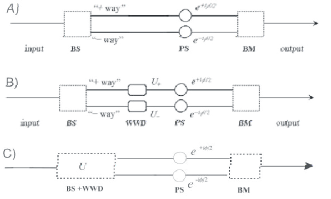
Figure 1: Schematic two-way interferometer setup, composed by: (a) A Beam splitter (BS), a Phase Shifter (PS) and a Beam Merger (BM). (b) The interferometer is supplemented with an additional quantum degree of freedom, the WWM, characterized by unitary $U_{\pm}$ evolution. (c) The unitary condition of $U_{\pm}$ is released to account for more general coupling to a WWM. Here, the evolution operator $U$ may exhibit non-unitary matrix elements.

IV Two-way interferometers with non-unitary WWM

Let us prepare the quanton initially in the state $s^{(0)}_{Q}=(0,0,s)$, where $-1\leq s\leq 1$ is the inversion footnote2 . Consider now the case plotted in Fig. 1(c). The state is given initially by $\rho^{(0)}=\rho_{Q}^{(0)}\otimes\rho_{M}^{(0)}$. The system evolves in time, $\rho^{(0)}\longrightarrow\rho^{(f)}=U^{\dagger}\rho^{(0)}U$ according to the unitary operator

$$U=\frac{1}{\sqrt{2}}\left(\begin{array}[]{cc}V_{++}&V_{+-}\\ -V_{-+}&V_{--}\end{array}\right),$$ (17)

where we have followed the notation given in Englert96b . Although $U$ is unitary, it might not be the case for its matrix elements separately. The particular case $V_{++}=V_{-+}=U_{+},\;V_{+-}=V_{--}=U_{-}$ recovers the situation described in Eq. (12).

The final state of the quanton, after application of all the transformation representing all the elements of the interferometer given in Fig. 1(c), is calculated in Jesus07 to be

$$\rho^{(f)}=\frac{1+s}{2}\;\rho^{(+)}+\frac{1-s}{2}\;\rho^{(-)},$$ (18)

with

$$\rho_{+}^{(f)}=\frac{1+\sigma_{x}}{4}V_{++}^{{\dagger}}\rho_{M}^{(0)}V_{++}+\frac{1-\sigma_{x}}{4}V_{+-}^{{\dagger}}\rho_{M}^{(0)}V_{+-}$$

$$-\frac{\sigma_{z}-i\sigma_{y}}{4}e^{-i\phi}V_{++}^{{\dagger}}\rho_{M}^{(0)}V_{+-}-\frac{\sigma_{z}+i\sigma_{y}}{4}e^{i\phi}V_{+-}^{{\dagger}}\rho_{M}^{(0)}V_{++},$$

and $\rho_{-}^{(f)}$ is obtained from $\rho_{+}^{(f)}$ through the changes $V_{++}\rightarrow-V_{-+},\;V_{+-}\rightarrow V_{--}$. Tracing over the cavity field degree of freedom, the final Bloch vector of the quanton can be calculated to be

$$S_{Qx}^{(f)} = w_{+}-w_{-}\,,$$

$$S_{Qy}^{(f)} = \Re e\left[\mathcal{C}e^{-i\phi}\right],$$

$$S_{Qz}^{(f)} = i\Im m\left[\mathcal{C}e^{-i\phi}\right],$$ (20)

where $\phi$ is the phase induced by the phase shifter. The contrast factor reads

$$\mathcal{C}=\frac{1+s}{2}\;\mathcal{C}_{\uparrow}+\frac{1-s}{2}\;\mathcal{C}_{\downarrow},$$ (21)

where

$$\mathcal{C}_{\uparrow} \equiv i\;\mbox{tr}_{D}\,\left\{V_{++}^{{\dagger}}\rho_{D}^{(0)}V_{+-}\right\}=i\left<V_{+-}V_{++}^{{\dagger}}\right>_{0},$$

$$\mathcal{C}_{\downarrow} \equiv -i\;\mbox{tr}_{D}\,\left\{V_{-+}^{{\dagger}}\rho_{D}^{(0)}V_{--}\right\}=-i\left<V_{--}V_{-+}^{{\dagger}}\right>_{0}.$$ (22)

The general form of $\mathcal{P}$ and $\mathcal{V}$ has also been calculated in Jesus07 . They read

$$\mathcal{P}=|\omega_{+}-\omega_{-}|=|s^{(f)}_{Qx}|,$$ (23)

with

$$w_{+} = \frac{1+s}{4}\;\left<V_{++}V_{++}^{{\dagger}}\right>_{0}+\frac{1-s}{4}\;\left<V_{-+}V_{-+}^{{\dagger}}\right>_{0},$$

$$w_{-} = \frac{1+s}{4}\;\left<V_{+-}V_{+-}^{{\dagger}}\right>_{0}+\frac{1-s}{4}\;\left<V_{--}V_{--}^{{\dagger}}\right>_{0}.$$ (24)

and

$$\mathcal{V}=|\mathcal{C}|\leq 1.$$ (25)

Note that $\mathcal{V}_{0}$ does not factorize now in the right hand side of Eq. (25) as it did in Eq. (13). This fact opens the door to he possibility of obtaining an interference pattern from an unpolarized source ($\mathcal{V}_{0}=0$) that will be explored in the next section. Combining Eqs. (20) and (25) we have

$$\mathcal{V}^{2}=|s^{(f)}_{Qy}|^{2}+|s^{(f)}_{Qz}|^{2}.$$ (26)

Summing Eqs. (26) and (23) we get

$$|s^{(f)}_{Q}|^{2}=\mathcal{V}^{2}+\mathcal{P}^{2}.$$ (27)

We find that Eq. (27) is a general result, valid even in the case of non-unitary WWM. The final state of the WWM can be calculated after tracing $\rho^{(f)}$ over the quanton’s degree of freedom. It reads Jesus07

$$\rho_{M}^{(f)}=\text{tr}_{Q}\,\rho^{(f)}=\omega_{+}\;\rho_{M}^{(+)}+\omega_{-}\;\rho^{(-)}_{M},$$ (28)

where

$$w_{+}\rho_{M}^{(+)} = \text{tr}_{Q}\left\{\frac{1+\sigma_{x}}{2}\;\rho^{(f)}\right\}$$

$$= \frac{1+s}{4}\;V_{++}^{{\dagger}}\rho_{D}^{o}V_{++}+\frac{1-s}{4}\;V_{-+}^{{\dagger}}\rho_{D}^{o}V_{-+},$$

$$w_{-}\rho_{M}^{(-)} = \text{tr}_{Q}\left\{\frac{1-\sigma_{x}}{2}\;\rho^{(f)}\right\}$$ (29)

$$= \frac{1+s}{4}\;V_{+-}^{{\dagger}}\rho_{D}^{o}V_{+-}+\frac{1-s}{4}\;V_{--}^{{\dagger}}\rho_{D}^{o}V_{--}$$

are the contributions associated to each way.

In order to analyze the exchange of entropy between quanton and WWM we make use of the $EM$ measures introduced in Eq. (6). The purity of the final WWM state can be calculated with the help of Eqs. (28) and (29) in the form

$$P_{M}=\text{tr}\rho_{M}^{2}=\frac{(1+s)^{2}}{16}\;\left[\left<V_{++}V_{++}^{{\dagger}}\right>_{0}^{2}+\left<V_{+-}V_{+-}^{{\dagger}}\right>_{0}^{2}\right.$$

$$\left.+2\left<V_{++}V_{+-}^{{\dagger}}\right>_{0}\left<V_{+-}V_{++}^{{\dagger}}\right>_{0}\right]$$

$$+\frac{(1-s)^{2}}{16}\;\left[\left<V_{-+}V_{-+}^{{\dagger}}\right>_{0}^{2}+\left<V_{--}V_{--}^{{\dagger}}\right>_{0}^{2}\right.$$

$$\left.+2\left<V_{-+}V_{--}^{{\dagger}}\right>_{0}\left<V_{--}V_{-+}^{{\dagger}}\right>_{0}\right]$$

$$+\frac{(1-s^{2})}{16}\;\left[2\left<V_{-+}V_{++}^{{\dagger}}\right>_{0}\left<V_{++}V_{-+}^{{\dagger}}\right>_{0}\right.$$

$$\left.+2\left<V_{--}V_{+-}^{{\dagger}}\right>_{0}\left<V_{+-}V_{--}^{{\dagger}}\right>_{0}\right.$$

$$\left.+2\left<V_{-+}V_{+-}^{{\dagger}}\right>_{0}\left<V_{+-}V_{-+}^{{\dagger}}\right>_{0}\right.$$

$$\left.+2\left<V_{++}V_{--}^{{\dagger}}\right>_{0}\left<V_{--}V_{++}^{{\dagger}}\right>_{0}\right]$$ (30)

For the quanton’s purity the calculation is much easier. Combining Eqs. (11) and (27), we have

$$P_{Q}=\frac{1}{2}(1+\mathcal{P}^{2}+\mathcal{V}^{2}).$$ (31)

V The Quantum Optical Ramsey interferometer

We particularize now the formalism described in the previous section to the case of a quantum optical Ramsey interferometer (QORI). This system has been extensively studied in the literature, both theoretically Englert96b ; JesusJulio04 ; Scully91 and experimentally newHaroche2001 ; Maitre97 ; Rauschenbeutel99 . The interaction hamiltonian given by the standard Jaynes-Cummings model (JCM) jcm

$$\mathcal{H}=\hbar\Omega\left(\sigma_{+}a+\sigma_{-}a^{\dagger}\right),$$ (32)

where $\sigma_{+}=|e\rangle\langle g|$ and $\sigma_{-}=|g\rangle\langle e|$ are the ladder operators for a two level atomic system composed by an excited $|e\rangle$ and a ground $|g\rangle$ state. These operators interact with a coupling strength $\Omega$ (the Rabi frequency of the atomic transition) with a microwave cavity field mode described by the bosonic $a,\,a^{\dagger}$ annihilation and creation operators. Thus, a low loss cavity resonator acts jointly as a which-way marker (WWM) and a beam splitter (BS) [see Fig. 1(c)]. Before entering the cavity, the atom is prepared, say, in the upper level $|e\rangle$ (case $s=1$). The atom interacts resonantly with the cavity field, adding a photon to its quantized cavity mode if a transition to the lower level $|g\rangle$ occurs. Due to the low-loss factor of the resonator, the cavity field can keep track of the way taken by the atom since it can store for long times the energy quantum liberated in the atomic transition kuhr . Thus, the same interaction both splits the beam and makes the two “ways” distinguishable. Next is the turn of the phase shifter (PS)—in the guise, for example, of an external pulse of electric field applied at the central stage of the interferometer. Finally, a classical microwave field at the port of the interferometer supplies the beam merger (BM), effecting a $\pi/2$ pulse after resonant interaction with the atom. The final state of the atom is measured by means of state-selective field ionization techniques at the output port of the interferometer. By varying the phase $\phi$ in successive repetitions of the experiment, a fringe pattern can be built up in the detected probability for the atom to wind up in one state or the other.

The evolution operators of Eq. (17) are given here by phoenix ,

$$V_{++} = \sqrt{2}\;\cos\left(\Omega\tau\sqrt{aa^{{\dagger}}}\right)$$

$$V_{+-} = -i\sqrt{2}\;\frac{\sin\left(\Omega\tau\sqrt{aa^{{\dagger}}}\right)}{\sqrt{aa^{{\dagger}}}}a$$

$$V_{-+} = -V_{+-}^{\dagger}$$

$$V_{--} = V_{++}^{\dagger}$$ (33)

where $\tau$ is the interaction time (the time of flight of the atom through the resonator).

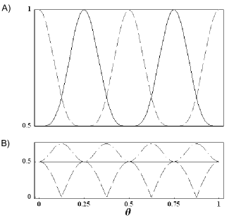
Figure 2: (a) $P_{Q}$ (solid curve) and $P_{M}$ (dashed curve). (b) Each one of the three terms in Eq. (34): $|\mathcal{G}_{Q}-\mathcal{G}_{M}|$ (dashed), $\mathcal{G}$ (solid) and $\mathcal{G}_{Q}+\mathcal{G}_{M}$ (dot-dashed). Both plots are shown as functions of the vacuum Rabi phase $\theta$ for $\overline{n}_{o}=0$ and $s=0$.

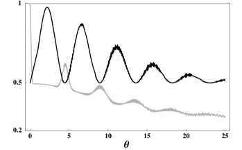
Figure 3: $P_{Q}$ (black curve) and $P_{M}$ (grey curve) as functions of the vacuum Rabi phase $\theta$ for $\overline{n}_{o}=20$ and $s=0$.

Consider now the cavity field prepared in the vacuum state so that the mean photon number is $\overline{n}_{0}=0$. The results for the purity of both subsystems (Eqs. (30) and (31)) are shown in Fig. 2 versus the normalized Rabi phase $\theta=\Omega\tau/{2\pi}$. Fig. 2(a) displays the dynamical process of purity swapping sudarshan . Here, the Bloch vector of the quanton oscillates in lenght in counterphase with the purity of the cavity field. As seen in the plot, both systems interchange purity periodically, with a period $T=\pi/\Omega$. This interchange is bounded by an Araki-Lieb type inequality as can be seen in Fig. 2(b) where the inequality

$$|\mathcal{G}_{Q}-\mathcal{G}_{M}|\leq\mathcal{G}\leq\mathcal{G}_{Q}+\mathcal{G}_{M}$$ (34)

is satisfied at all times. Moreover, we have numerically confirmed that Eq. (34) is satisfied for a dense grid of values of $(s,\,\overline{n}_{0},\,\theta)$ footnote5 . This result supports the conjecture given in Eq. (1). Note in Fig. 2(b) that the points of maximal purity interchange makes Eq. (34) an equality. The oscillations shown in Fig. 2(a) are similar to those found in sudarshan for a pair of qubits coupled by a nonlocal interaction.

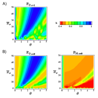
Figure 4: Contour plots of $P_{Q}$ and $P_{M}$ as functions of the cavity field’s intensity $\overline{n}_{0}$ and the vacuum Rabi phase $\theta$. Plots are shown for two different initial preparations of the quanton’s state. (a) The plot on first line belongs to pure state preparation ($s=1$). (b) The remaining two plots belong to a totally mixed state preparation ($s=0$).

But, what happens when we inject to the cavity field more and more photons? In a typical experimental situation, the cavity field is prepared in a coherent state with a large $\overline{n}_{0}$ raimond . We find that purity swapping is still obtained. The oscillations become damped and more irregular, since the dynamics mixes different phases stemming from different photon manifolds. The $P_{M}$ envelope decreases with $\theta$, indicating that more photon manifolds get entangled as the number of Rabi floppings increases. This is shown in Fig. 3 where $P_{Q,M}$ are plotted for $s=0$ and $\overline{n}_{0}=20$. What we see here are manifestations of the collapses and revivals of the JCM Gea90 . The first plateau in $P_{M}$ corresponds to the collapse region ($\mathcal{P}\rightarrow 0$). In these zones, $P_{Q}$ follows the behavior of the visibility $\mathcal{V}$. We show this explicitely in Fig. 4, where $P_{Q,M}$ is plotted for different preparations of $\overline{n}_{0}$ and $\theta$.

On one hand, Fig. 4(a) shows results for initial pure state preparation of the quanton ($s=1$). Here $P_{Q}=P_{M}$. We can understand this effect in terms the Araki-Lieb inequality given in Eq. (34). After Eq. (7) we have $\mathcal{G}^{(0)}=0$. The purity is conserved under unitary $U$ global evolution, so $\mathcal{G}^{(f)}=0$. According to Eq. (34), $\mathcal{G}_{Q}=\mathcal{G}_{M}$ at all times. Apart from Eq. (34), this property can also be derived from the general properties of $EM$. In fact, not only the entropy of entanglement but all $EM$ for pure states are symmetric under the exchange of parties vidal2000 . Another main feature of Fig. 4 can be easily related to the properties of $EM$. In fact, for every $EM$ measure vidal2000

$$EM(\rho)\geq 0.$$ (35)

For a separable state $\rho_{QM}$, $EM(\rho_{QM})=0$. This is what occurs at the $P_{Q}\rightarrow 1$ zone of Fig. 4(a). The dynamics decouples $\rho_{Q}$ and $\rho_{M}$ asymptotically in the recreation zone defined by the relation

$$\theta_{R}=\sqrt{\overline{n}_{0}}.$$ (36)

Here Eq. (7) is satisfied and reduces to $\mathcal{G}_{Q,M}=0$, so $P_{Q}=P_{M}\rightarrow 1$. The linear entropy properties as an $EM$ accounts for the recreation of state vector phenomena for $s=1$ found by Gea-Banacloche Gea90 .

On the other hand, new results are shown in Fig. 4(b) for the case of a initial totally unpolarized quanton state (s=0). Remarkably, we obtain here as well an asymptotically recreation of the state vector $P_{Q}\rightarrow 1$ in the first recreation zone. This is apparent comparing the plots for ${P_{Q}}_{s=1}$ and ${P_{Q}}_{s=0}$ in Fig. 4(a) and Fig. 4(b). Here, it can be seen that many revival zones wash out in the lower plot. However, the recreation of the state vector in the first zone $\theta_{R}$ is robust against degradation of the initial purity of the quanton, given by $s$ (i.e., $P_{Q}^{(0)}=\frac{1}{2}(1+s^{2})$). This is one of the main results of the paper.

This results contrast the unitary WWM case, where $P_{Q}^{(0)}=0$ implies $P_{Q}^{(f)}=0$ at all times (see Eq. (16)). Contrary to this, we obtain here that the JCM interaction can result in a significant increase of the visibility of a totally unpolarized quanton. This can be seen in the right plot of Fig. 5(b), where the visibility for $s=0$ is explicitly plotted in the same fashion as Fig. 4. The blue zone gives a wide region for experimentalists willing to obtain perfect interference patterns starting from totally unpolarized sources. We can understand this phenomena by recalling again Eq. (34). According to Eq. (7), $\mathcal{G}_{Q}^{(0)}=\mathcal{G}^{(0)}>0$, since we start now with a mixed quanton’s state. Eq. (34) allows a net transfer of entropy build up from the quanton to the cavity field. $P_{Q}\simeq 1$ can arise at the expenses of maximally increasing the entropy of the cavity field. This can be seen comparing $P_{Q}$ and $P_{M}$ in Fig. 4(b). The quanton gets pure $P^{(0)}_{Q}=1/2\longrightarrow P^{(f)}_{Q}=1$ at the expense of a reciprocal increase of the entropy of the interacting system $P^{(0)}_{M}=1\longrightarrow P^{(f)}_{M}=1/2$. This maximal purity swapping is consistent with the Araki-Lieb bounds of Eq. (34). In fact, they are not only consistent but demanded by it. In order to see this, let us insert Eqs. (6) and (8) into Eq. (34) for $s=0$. We have

$$|P_{M}-P_{Q}|\leq\frac{1}{2}\leq 2-P_{M}-P_{Q}.$$ (37)

Eq. (37) sets up the bounds of purity exchange between the systems. This bounds can be observed in the results given in Figs. (2-4). These are strong bounds and provide useful information. For instance as $P_{Q}\rightarrow 1$, it is easy to show that Eq. (37) demands $P_{M}\rightarrow 1/2$.

Both subsystems decouple in the recreation zone asymptotically with $\overline{n}_{0}$ for all values of $s$. The mutual information

$$\mathcal{I}=\mathcal{G}_{Q}+\mathcal{G}_{M}-\mathcal{G}_{Q}\mathcal{G}_{M}-\mathcal{G}$$ (38)

is plotted in Fig. 5. It can be seen that for $s=0$ less entanglement and wider zones of decoupling are obtained in comparison to $s=1$. It can also be noticed in Fig. 5(b) that even if we start from a totally mixed quanton state, an appreciable amount of entanglement can build up at long times for low values of $\overline{n}_{0}$.

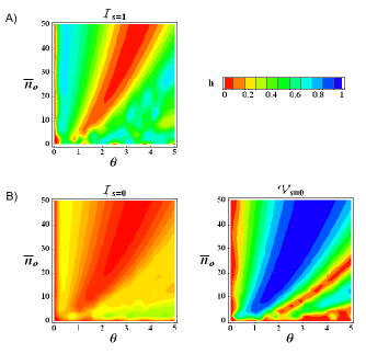
Figure 5: Mutual information of the combined system and fringe visibility as functions of the cavity field’s intensity $\overline{n}_{o}$ and the vacuum Rabi phase $\theta$. Plots are shown for two different initial preparations of the quanton’s state: (a) pure and (b) totally unpolarized.

Finally, we connect our results with the robustness of the Gea attractor. Julio Gea-Banacloche Gea90 studied the $s=1$ case. At the beginning of its evolution, the quanton becomes rapidly unpolarized (collapse region), but right after the quanton evolves to the form of the pure state attractor

$$\left|\Psi\right\rangle_{Q}^{attr}=\frac{1}{\sqrt{2}}(\left|e\right\rangle+\,i\,e^{i\alpha}\left|g\right\rangle),$$ (39)

where $\alpha$ is the phase of the cavity field. The above attractor state arises at the half of the revival time leading to the recreation of the state vector. As was demonstrated in Gea90 , the state of any initial totally polarized atom ($s=1$ case) will evolve to the attractor state, regardless of any other atomic initial conditions.

Now, we show that the Gea-Banacloche attractor state is reached also for any initial purity of the state. Towards this goal we calculate the state just after the beam splitter. We can undo the action of the beam merger by taking the transformation on Eqs. (IV)

$$\sigma_{x}\rightarrow\sigma_{z},\;\;\sigma_{z}\rightarrow-\sigma_{x}.$$ (40)

With these transformations, taking $\phi=0$ and taking the trace of the resulting total state over the WWM’s degree of freedom we obtain the quanton’s state just after the beam splitter

$$\rho_{Q}^{BS}=\frac{1}{2}\left(1-i\sigma_{x}\Im m\left[\mathcal{C}\right]+\sigma_{y}\Re e\left[\mathcal{C}\right]+\sigma_{z}\mathcal{P}\right),$$ (41)

where $\mathcal{P}$ and $\mathcal{C}$ were already defined in Eqs. (10) and (21). Now we particularize the above state to the recreation zone given by Eq. (36). As seen in Fig. 4(b), here $\mathcal{V}\rightarrow 1$. Thus $\mathcal{P}\rightarrow 0$, since $\mathcal{V}^{2}+\mathcal{P}^{2}\leq 1$. Therefore, using Eq. (25) it is easy to show that in the recreation zone Eq. (41) tends to Eq. (39), once $\alpha$ is defined as the phase of the complex contrast factor $\mathcal{C}$ footnote6 . The quanton state evolves to the pure state Gea-Banacloche attractor, gaining purity at the expense of increasing the entropy on the cavity field, which gets decoupled from the quanton in the process. Note that in this calculation we did not particularize at anytime for any initial quanton’s state. Thus, we have generalized the result from Gea90 and demonstrated that the Gea-Banacloche attractor is robust against all quanton’s initial conditions, including degradation of the purity of the quanton.

VI Conclusions

In conclusion, we have shown the existence of dynamical purity swapping in the JCM. The dynamic itself purifies the qubit at the expense of degrading the purity of the cavity field. Moreover, we have shown that a qubit can exhibit dynamical purity swapping with a generic quantum system, provided they coupled via a non-unitary matrix elements interaction [in the sense of Eq. (17)]. We have been able to obtain such general necessary condition for purity swapping thanks to an interferometric approach, allowing us to connect purity degradation with which-way marking. Then we have analyzed in detail the particular case of the JCM, since it describes a large variety of systems. It also serves as a cornerstone for experimental quantum information, communication and computing. In fact, the observation of this phenomena is perfectly attainable with current technology newHaroche2001 . We have shown that the Gea-Banacloche attractor is robust against degradation of the initial purity of the quanton. Any initially totally unpolarized qubit will evolve to the pure state Gea-Banacloche attractor after interacting with the cavity field the time required by Eq. (36). Thus, we can use the collapses and revivals phenomena of the JCM for dynamical purification of qubits. Since the field’s phase $\alpha$ in Eq. (39) is an externally controllable parameter, this phenomena can also be used for quantum preparation of pure superposition states starting from totally mixed states. This demonstrates in addition the possibility of a remarkable phenomena: the arising of a perfect visibility interference pattern starting from a totally unpolarized source of qubits. Finally, we show that the Tsallis entropy $T_{2}$ is a useful entanglement monotone ($EM$) allowing one to relate entanglement with purity swapping. Many features of the phenomena have been shown to derive from the algebraic properties of $EM$.

- (1) B. W. Shore and P. L. Knight, J. Mod. Opt. 40, 1195-1238 (1993).
- (2) I. Wilson-Rae and A. Imamoglu, Phys. Rev. B 65 235311 (2002); G. S. Solomon, M. Pelton and Y. Yamamoto, Phys. Rev. Lett. 86, 3903 (2001).
- (3) A. Blais, R.-S. Huang, A. Wallraff, S. M. Girvin and R. J. Schoelkopf, Phys. Rev. A 69, 062320 (2004).
- (4) P. Berman, ”Cavity Quantum Electrodynamics”, Academic Press, Boston, MA (1994).
- (5) E. Hagley et al., Phys. Rev. Lett. 79, 1 (1997); A. Rauschenbeutel, P. Bertet, S. Osnaghi, G. Nogues, M. Brune, J. M. Raimond and S. Haroche, Phys. Rev. A 64, 050301 (R) (2001).
- (6) G. R. Guthohrlein, M. Keller, K. Hayasaka, W. Lange, and H. Walther, Nature 414, 49 (2001).
- (7) A. B. Mundt, A. Kreuter, C. Becher, D. Leibfried, J. Eschner, F. Schmidt-Kaler, and R. Blatt, Phys. Rev. Lett. 89, 103001 (2002).
- (8) J. M. Raimond, M. Brune, and S. Haroche, Rev. Mod. Phys. 73, 565 (2001).
- (9) M. A. Nielsen and I. L. Chuang, ”Quantum Computation and Quantum Information”, Cambridge University Press (2000).
- (10) M.R. Gallis, Phys. Rev. A 53, 655 (1996).
- (11) To our knowledge, this inequality has not yet been proved.
- (12) J. Martinez-Linares and D.A. Harmin, Phys. Rev. A69, 062109 (2004).
- (13) J. Martinez-Linares, Phys. Rev. A75, 052112 (2007).
- (14) S. Popescu and D. Rohrlich, Phy. Rev. A 56, R3319 (1997).
- (15) C.H. Bennett, G. Brassard, S. Popescu, B. Schumacher, J.A. Smolin and W.K. Wootters, Phys. Rev. Lett. 76, 722 (1996). C.H. Bennett, H.J. Bernstein, S. Popescu, and B. Schumacher, Phys. Rev. A 53, 2046 (1996).
- (16) H. Araki, E. Lieb. Commun. Math. Phys. 18, 160-170 (1970).
- (17) C.H. Bennett, D.P.DiVincenzo, J.A. Smolin, and W.K. Wootters, Phys. Rev. A 54, 3824 (1996); G. Vidal and J. I. Cirac, Phys. Rev. Lett. 86, 5803 (2001); V. Vedral, Rev. Mod. Phys. 74, 197 (2002); G. Vidal and R. Tarrach, Phys. Rev. A 59, 141 (1999).
- (18) G. Vidal, J. Mod. Opt. 47, 355 (2000).
- (19) A. Wehrl, Rev. Mod. Phys. 50, 221 (1978).
- (20) C. Tsallis, J. Stat. Phys. 52, 479 487 (1988).
- (21) G.A. Raggio, J. Math. Phys. 36, 4785 4791 (1995).
- (22) G. Vidal, Phys. Rev. Lett. 83, 1046 (1999).
- (23) B.-G. Englert, Phys. Rev. Lett. 77, 2154 (1996).
- (24) Starting with a balanced beam splitter, the only source of assymetry comes from a non-zero .
- (25) As noted in Englert96b , there is no need to consider more generic Bloch vector, since this just amounts to a redefinition of the operators in Eq. (17).
- (26) B.-G. Englert, Acta Phys. Slov. 46, 249 (1996).
- (27) J. Martinez-Linares and J. Vargas-Medina. Journal of Optics B: Quantum and Semiclassical Optics. 6 S560-S565 (2004).
- (28) This resonant scheme was initially proposed in M. O. Scully, B.-G. Englert, and H. Walther, Nature 351, 111 (1991).
- (29) P. Bertet et al., Nature 411, 166 (2001).
- (30) X. Maître et al., Phys. Rev. Lett. 79, 769 (1997).
- (31) A. Rauschenbeutel et al., Phys. Rev. Lett. 83, 5166 (1999).
- (32) E. T. Jaynes, F. W. Cummings, Proc. IEEE 51, 89 (1963).
- (33) Up to 100 Rabi floppings, as can be seen in: S. Kuhr, S. Gleyzes, C. Guerlin, J. Bernu, U. B. Hoff, S. Del glise, S. Osnaghi, M. Brune, J. M. Raimond, S. Haroche, E. Jacques, P. Bosland and B. Visentin, quant-ph/0612138v2.
- (34) S. J. D. Phoenix and P. L. Knight, Ann. Phys. (N. Y.) 186, 381 (1998).
- (35) C. A. Rodriguez, A. Shaji and E. C. G. Sudarshan, quant-phys/0504051v4.
- (36) We have checked Eq. (34) over 1600 points in the interval , .
- (37) J. Gea-Banacloche, Phys. Rev. Lett. 65, 3385 (1990); Phys. Rev. A 44, 5913 (1991).
- (38) In fact, according to Eqs. (22) and (33) can be shown to be the phase of the cavity field.