Abstract

We study the capabilities of future electron-positron Linear Colliders, with centre-of-mass energy at the TeV scale, in accessing the parameter space of a $Z^{\prime}$ boson within the minimal $B-L$ model. In such a model, wherein the Standard Model gauge group is augmented by a broken $U(1)_{B-L}$ symmetry – with $B(L)$ being the baryon(lepton) number – the emerging $Z^{\prime}$ mass is expected to be in the above energy range. We carry out a detailed comparison between the discovery regions mapped over a two-dimensional configuration space ($Z^{\prime}$ mass and coupling) at the Large Hadron Collider and possible future Linear Colliders for the case of di-muon production. As known in the literature for other $Z^{\prime}$ models, we confirm that leptonic machines, as compared to the CERN hadronic accelerator, display an additional potential in discovering a $B-L$ $Z^{\prime}$ boson as well as in allowing one to study its properties at a level of precision well beyond that of any of the existing colliders.

1 Introduction

The $B-L$ (baryon number minus lepton number) symmetry plays an important role in various physics scenarios beyond the Standard Model (SM). Firstly, the gauged $U(1)_{B-L}$ symmetry group is contained in a Grand Unified Theory (GUT) described by a $SO(10)$ group [1]. Secondly, the scale of the $B-L$ symmetry breaking is related to the mass scale of the heavy right-handed Majorana neutrino mass terms providing the well-known see-saw mechanism [2] of light neutrino mass generation. Thirdly, the $B-L$ symmetry and the scale of its breaking are tightly connected to the baryogenesis mechanism through leptogenesis [3] via sphaleron interactions preserving $B-L$.

The minimal $B-L$ low-energy extension of the SM consists of a further $U(1)_{B-L}$ gauge group, three right-handed neutrinos and an additional Higgs boson generated through the $U(1)_{B-L}$ symmetry breaking. It is important to note that in this model the ${B-L}$ breaking can take place at the TeV scale, i.e. far below that of any GUT. This $B-L$ scenario therefore has interesting implications at the Large Hadron Collider (LHC), including new clean signatures from $Z^{\prime}$, Higgs bosons and heavy neutrinos [4]–[5].

In the present paper we study the phenomenology related to the $Z^{\prime}$ sector of the minimal $B-L$ extension of the SM at the new generation of $e^{+}e^{-}$ Linear Colliders (LCs) [6]. We consider the $e^{+}e^{-}\to\mu^{+}\mu^{-}$ channel as a representative process in order to study new signatures pertaining to the $B-L$ model.

As it is well known (see, e.g., Refs. [7] and [8]), the LC environment is one of the most suitable for $Z^{\prime}$ physics, for two main reasons. First, if a $Z^{\prime}$ is found at the LHC, it could be the case that the underlying model is hard to identify at the hadronic machine; in contrast, the clean experimental environment of a LC is the ideal framework to establish the $Z^{\prime}$ line-shape (i.e. its mass and width) and to measure its couplings, thereby identifying the model and the observed spin$-1$ boson [9]. Second, we will also show that there exists further scope for a LC operating at TeV energies: specifically, to discover a $Z^{\prime}$ boson over regions of the $B-L$ parameter space which cannot be probed at all at the LHC, either directly through a resonance (when $\sqrt{s}_{e^{+}e^{-}}\geq M_{Z^{\prime}}$) or indirectly through interference effects (when $\sqrt{s}_{e^{+}e^{-}}<M_{Z^{\prime}}$). In both instances, a LC proves to be more powerful than the LHC in accessing the region of small $Z^{\prime}$ couplings.

This work is organised as follows. In the next section we describe the model. In Sect. 3 we illustrate the computational techniques adopted. In Sect. 4 we present our numerical results. The conclusions are in Sect. 5.

2 The model

The model under study is the so-called “pure” or “minimal” $B-L$ model (see [4] for conventions and references) since it has vanishing mixing between the two $U(1)_{Y}$ and $U(1)_{B-L}$ groups. In the rest of this paper we refer to this model simply as the “$B-L$ model”. In this model the classical gauge invariant Lagrangian, obeying the $SU(3)_{C}\times SU(2)_{L}\times U(1)_{Y}\times U(1)_{B-L}$ gauge symmetry, can be decomposed as:

$$\mathscr{L}=\mathscr{L}_{YM}+\mathscr{L}_{s}+\mathscr{L}_{f}+\mathscr{L}_{Y}\,.$$ (1)

The non-Abelian field strengths in $\mathscr{L}_{YM}$ are the same as in the SM whereas the Abelian ones can be written as follows:

$$\mathscr{L}^{\rm Abel}_{YM}=-\frac{1}{4}F^{\mu\nu}F_{\mu\nu}-\frac{1}{4}F^{\prime\mu\nu}F^{\prime}_{\mu\nu}\,,$$ (2)

where

$$F_{\mu\nu} = \partial_{\mu}B_{\nu}-\partial_{\nu}B_{\mu}\,,$$ (3)

$$F^{\prime}_{\mu\nu} = \partial_{\mu}B^{\prime}_{\nu}-\partial_{\nu}B^{\prime}_{\mu}\,.$$ (4)

In this field basis, the covariant derivative is:

$$D_{\mu}\equiv\partial_{\mu}+ig_{S}T^{\alpha}G_{\mu}^{\phantom{o}\alpha}+igT^{a}W_{\mu}^{\phantom{o}a}+ig_{1}YB_{\mu}+i(\widetilde{g}Y+g_{1}^{\prime}Y_{B-L})B^{\prime}_{\mu}\,.$$ (5)

The “pure” or “minimal” $B-L$ model is defined by the condition $\widetilde{g}=0$, that implies no mixing between the $Z^{\prime}$ and the SM-$Z$ gauge bosons.

The fermionic Lagrangian (where $k$ is the generation index) is given by

$$\mathscr{L}_{f} = \sum_{k=1}^{3}\Big{(}i\overline{q_{kL}}\gamma_{\mu}D^{\mu}q_{kL}+i\overline{u_{kR}}\gamma_{\mu}D^{\mu}u_{kR}+i\overline{d_{kR}}\gamma_{\mu}D^{\mu}d_{kR}+$$ (6)

$$+i\overline{l_{kL}}\gamma_{\mu}D^{\mu}l_{kL}+i\overline{e_{kR}}\gamma_{\mu}D^{\mu}e_{kR}+i\overline{\nu_{kR}}\gamma_{\mu}D^{\mu}\nu_{kR}\Big{)}\,,$$

where the fields’ charges are the usual SM and $B-L$ ones (in particular, $B-L=1/3$ for quarks and $-1$ for leptons). The $B-L$ charge assignments of the fields as well as the introduction of new fermionic right-handed heavy neutrinos ($\nu_{R}$) and scalar Higgs ($\chi$, charged $+2$ under $B-L$) fields are designed to eliminate the triangular $B-L$ gauge anomalies and to ensure the gauge invariance of the theory (see eq. (9)), respectively. Therefore, the $B-L$ gauge extension of the SM group broken at the EW scale does necessarily require at least one new scalar field and three new fermionic fields which are charged with respect to the $B-L$ group.

The scalar Lagrangian is:

$$\mathscr{L}_{s}=\left(D^{\mu}H\right)^{\dagger}D_{\mu}H+\left(D^{\mu}\chi\right)^{\dagger}D_{\mu}\chi-V(H,\chi)\,,$$ (7)

with the scalar potential given by

$$V(H,\chi)=m^{2}H^{\dagger}H+\mu^{2}\mid\chi\mid^{2}+\lambda_{1}(H^{\dagger}H)^{2}+\lambda_{2}\mid\chi\mid^{4}+\lambda_{3}H^{\dagger}H\mid\chi\mid^{2}\,,$$ (8)

where $H$ and $\chi$ are the complex scalar Higgs doublet and singlet fields, respectively.

Finally, the Yukawa interactions are:

$$\mathscr{L}_{Y} = -y^{d}_{jk}\overline{q_{jL}}d_{kR}H-y^{u}_{jk}\overline{q_{jL}}u_{kR}\widetilde{H}-y^{e}_{jk}\overline{l_{jL}}e_{kR}H$$ (9)

$$-y^{\nu}_{jk}\overline{l_{jL}}\nu_{kR}\widetilde{H}-y^{M}_{jk}\overline{(\nu_{R})^{c}_{j}}\nu_{kR}\chi+{\rm h.c.}\,,$$

where $\tilde{H}=i\sigma^{2}H^{*}$ and $i,j,k$ take the values $1$ to $3$, where the last term is the Majorana contribution and the others the usual Dirac ones.

3 Calculation

The study we present in this paper has been performed with the help of the CalcHEP package [10], in which the model under discussion had been previously implemented via the LanHEP tool [11], as already discussed in [4].

A feature specific to LCs is the presence of Initial State Radiation (ISR) and Beamstrahlung. For the former, CalcHEP [12] implements the Jadach, Skrzypek and Ward expressions of Ref. [13]. Regarding the latter, we adopted the parameterisation specified for the International Linear Collider (ILC) project in [9]:

Horizontal beam size (nm) $$= 640,$$

Vertical beam size (nm) $$= 5.7,$$

Bunch length (mm) $$= 0.300,$$

Number of particles in the bunch (N) $$= 2\times 10^{10}.$$ (10)

There exists a certain subtlety in the comparison of the LHC and LC discovery potentials of a $Z^{\prime}$ boson. This comparison is not straightforward and ought to be performed carefully [14]–[15]. First of all, we need to compare consistent temporal collections of data. On the one hand, luminosities are different at the two kind of machines and so are supposed to be the running schedules. Besides, in this work, we also consider the fact that, while at the LHC we will have essentially a fixed beam energy technology, at LCs one can afford the possibility of beam energy scans. In this connection, while comparing the scope of the two, we have assumed 100 fb^-1 for the LHC throughout and 500(10) fb^-1 for LCs running at fixed energy (in energy scanning mode). On the other hand, data samples will be collected differently, chiefly, acceptance and selection procedures will be different. In this connection, we have assumed standard acceptance cuts (on muons) at the LHC and a typical LC,

$${\rm LHC:}\qquad p_{T}^{\mu} > 10~{}{\rm GeV},\qquad|\eta^{\mu}|<2.5,$$ (11)

$${\rm LC:}\qquad E^{\mu} > 10~{}{\rm GeV},\qquad|\cos\theta^{\mu}|<0.95.$$ (12)

Then, for both signal and background, we apply the following cut on the di-muon invariant mass, $M_{\mu\mu}$:

$${\rm LHC:}\qquad|M_{\mu\mu}-M_{Z^{\prime}}| < \mbox{max}\left(3\Gamma_{Z^{\prime}},\;\left(0.03\sqrt{\frac{M_{Z^{\prime}}}{\rm GeV}}+0.005\frac{M_{Z^{\prime}}}{\rm GeV}\right){\rm GeV}\;\right),$$ (13)

$${\rm LC:}\qquad|M_{\mu\mu}-M_{Z^{\prime}}| < \mbox{max}\left(3\Gamma_{Z^{\prime}},\;0.15\sqrt{\frac{M_{Z^{\prime}}}{\rm GeV}}{\rm GeV}\;\right),$$ (14)

that is, a half window as large as either three times the width of the $Z^{\prime}$-boson or the di-muon mass resolution, whichever the largest.

In our analysis we implement a suitable definition of signal significance, applicable to both the LHC and LC contexts, which we have done as follows. In the region where the number of both signal ($s$) and background ($b$) events is large enough (bigger than 20), we use a definition of significance based on Gaussian statistics, ${\sigma}\equiv{\it s}/{\sqrt{b}}$. Otherwise, in case of lower statistics, we exploited the Bityukov algorithm [18], which basically uses the Poisson ‘true’ distribution instead of the approximated Gaussian one. Hereafter, to ‘Observation’ it will correspond the condition $\sigma\geq 3$ and to ‘Discovery’ $\sigma\geq 5$.

Finally, as in [4], in the LHC case we used CTEQ6L [19], with $Q^{2}=M_{Z^{\prime}}^{2}$, as default Parton Distribution Functions (PDFs).

4 Results

Hereafter, we assume that the heavy neutrinos and Higgs states of the model have masses as in [4]. This choice of the parameters only affects the $Z^{\prime}$ width, in fact minimally (a few percents), so that our conclusions will be unchanged by it. Regarding the possible phenomenology of the new neutrino states, the relatively small cross sections involving the production of the latter require very high luminosity to become important, especially for very small values of the couplings, hence beyond the scope of the present paper. Concerning the Higgs sector, we are currently in the process of defining the accessible parameter space (subject to experimental and theoretical constraints) ameanable to phenomenological analysis [20]. The Higgs mass choices made here are then meant to be illustrative of the case in which the Higgs sector of the model impinges marginally on $Z^{\prime}$ phenomenology.

4.1 Experimental limits on $Z^{\prime}$ masses and couplings in $B-L$

Before proceeding to our signal-to-background analysis, we ought to define the parameter space of the $B-L$ model sector, compliant with current experimental constraints. Some stringent ‘indirect’ limits on the $Z^{\prime}$ mass-to-coupling ratio can be extracted from precision data (obtained at LEP and SLC), where the use of a four-fermion interaction already gives rather accurate results [21]. Despite this approach is well established, it is worth to note that more sophisticated techniques could change such bounds. However, in the course of our analysis, we will be constraining ourselves to regions of masses and couplings that are immune from such constraints, as they lie well beyond the LEP and SLC limits (as well illustrated in some of our plots). Since the approximation used for the extraction of such limits is therefore irrelevant, we decided to quote and adopt here the more conservative result obtained by [22]:

$$\frac{M_{Z^{\prime}}}{g^{\prime}_{1}}\geq 7\;\rm{TeV}\,$$ (15)

(which is not significantly lowered in the analysis of [21]: where $M_{Z^{\prime}}/g^{\prime}_{1}\geq 6$ TeV is quoted). The most constraining ‘direct’ bounds come from Run 2 at Tevatron, chiefly from $q\overline{q}\rightarrow\mu^{+}\mu^{-}$ analyses. For definiteness, we take the CDF analysis of Ref. [23] using $2.3\,\mbox{fb}^{-1}$ of data, which sets lower limits for $Z^{\prime}$ masses coming from several scenarios (e.g., a SM-like $Z^{\prime}$ and some $E_{6}$ string-inspired $Z^{\prime}$ models), but not for the $B-L$ case. Nonetheless, by rescaling the SM-like $Z^{\prime}$ coupling, we get for our $B-L$ setup, at $95\%$ C.L., the lower bounds displayed in Tab. 1.

$g_{1}^{\prime}$	$M_{Z^{\prime}}$ (GeV)
0.065	600
0.075	680
0.090	740
0.1	800
0.2	960
0.5	1140

Table 1: Lower bounds on the $Z^{\prime}$ mass for selected $g_{1}^{\prime}$ values in our $B-L$ model, at $95\%$ C.L., by rescaling the SM-like $Z^{\prime}$ coupling of Ref. [23].

4.2 The LHC and LC potential in detecting $Z^{\prime}$ bosons in $B-L$

We start the presentation of our results by showing Fig. 1, which demonstrates the LHC and ILC discovery potential of a $Z^{\prime}$ boson over the $M_{Z^{\prime}}$-$g_{1}^{\prime}$ plane. Here, we define the signal as di-muon production via $Z^{\prime}$ exchange together with its interferences with the SM (i.e., $\gamma$ and $Z$ exchange) sub-processes whereas as background we take the SM di-muon production via $\gamma$ and $Z$ exchange. Both signal and background are then limited to the detector acceptance volumes and $M_{\mu\mu}$ invariant mass window described in the previous section. In Fig. 1a we considered a LC collecting data at the fixed energy of $\sqrt{s_{e^{+}e^{-}}}=3$ TeV. As one can clearly see, for $M_{Z^{\prime}}>800$ GeV, the LC potential to explore the $M_{Z^{\prime}}$-$g_{1}^{\prime}$ parameter space goes beyond the LHC reach. For example, for $M_{Z^{\prime}}=1$ TeV, the LHC can discover a $Z^{\prime}$ if $g^{\prime}\approx 0.007$ while a LC can achieve this for $g^{\prime}\approx 0.005$. The difference is even more drastic for larger $Z^{\prime}$ masses as one can see from Tab. 2: a LC can discover a $Z^{\prime}$ with a $2$ TeV mass for a $g_{1}^{\prime}$ coupling which is a factor 8 smaller than the one for which the same mass $Z^{\prime}$ can be discovered at the LHC.

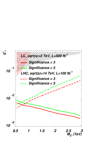
(a)

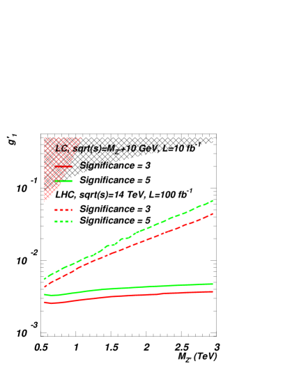
(b)

Figure 1: Significance contour levels plotted against $g_{1}^{\prime}$ and $M_{Z^{\prime}}$ both at the LHC for $L=100\;{\rm fb}^{-1}$ ($\sqrt{s_{pp}}=14$ TeV, dotted line) and (1a) a LC for $L=500\;{\rm fb}^{-1}$, $\sqrt{s_{e^{+}e^{-}}}=3$ TeV plus (1b) a LC for $L=10\;{\rm fb}^{-1}$, $\sqrt{s_{e^{+}e^{-}}}=M_{Z^{\prime}}+10$ GeV, both in continuous line. The shaded areas correspond to the region of parameter space excluded experimentally, in accordance with eq. (15) (LEP bounds, in black) and Tab. 1 (Tevatron bounds, in red).

$M_{Z^{\prime}}$ (TeV)	$g_{1}^{\prime}$
	LHC	LC ($\sqrt{s}=3$ TeV)	LC ($\sqrt{s}=M_{Z^{\prime}}+10$ GeV)
1.0	0.0071	0.0050	0.0026
1.5	0.011	0.0040	0.0032
2.0	0.018	0.0028	0.0034
2.5	0.028	0.0022	0.0035

Table 2: Minimum $g_{1}^{\prime}$ value accessible at the LHC and a LC for selected $M_{Z^{\prime}}$ values in our $B-L$ model. At the LHC we assume $L=100\;{\rm fb}^{-1}$ whereas for a LC we take $L=500\;{\rm fb}^{-1}$ at fixed energy and $L=10\;{\rm fb}^{-1}$ in energy scanning mode.

In case of the energy scan approach, when the LC energy is set to $\sqrt{s_{e^{+}e^{-}}}=M_{Z^{\prime}}+10$ GeV (assuming $10\mbox{ fb}^{-1}$ of luminosity for each step), the parameter space can be probed even further for $M_{Z^{\prime}}<1.75$ TeV, as shown in Fig. 1b. For example, for $M_{Z^{\prime}}=1$ TeV, $g_{1}^{\prime}$ couplings can be probed down to the $2.6\times 10^{-3}$, following a $Z^{\prime}$ discovery. Furthermore, one can see that the parameter space corresponding to the mass interval $500~{}{\rm GeV}~{}<M_{Z^{\prime}}<1$ TeV, which the LHC covers better as compared to a LC with fixed energy, can be accessed well beyond the LHC reach with a LC in energy scan regime. Altogether then, both an ILC, $\sqrt{s_{e^{+}e^{-}}}\leq 1$ TeV) [24] and a Compact Linear Collider (CLIC, $\sqrt{s_{e^{+}e^{-}}}\leq 3$ TeV) [25] design may be able (over suitable regions of $B-L$ parameter space) to outperform the LHC.

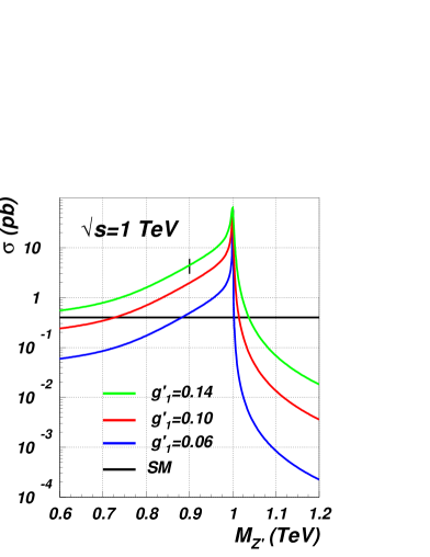
(a)

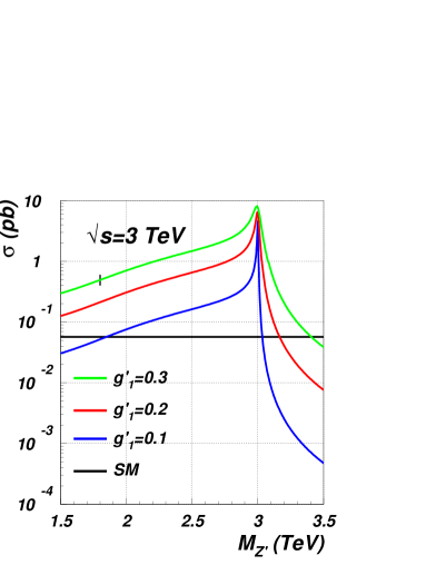
(b)

Figure 2: Cross section for the process $e^{+}e^{-}\rightarrow X\to\mu^{+}\mu^{-}$ for the signal ($X=Z^{\prime}$) and the SM background ($X=\gamma,Z$, independent from $M_{Z^{\prime}}$) plotted against $M_{Z^{\prime}}$ at (2a) a LC with $\sqrt{s_{e^{+}e^{-}}}=1$ TeV and (2b) a LC with $\sqrt{s_{e^{+}e^{-}}}=3$ TeV. (The black vertical bar refers to the mass and coupling combinations excluded by experimental data, to the left of it.)

Figs. 2a–2b present the general pattern of the $Z^{\prime}$ production cross section in comparison to the SM background as a function of $M_{Z^{\prime}}$, for two fixed values of $\sqrt{s_{e^{+}e^{-}}}$, in such configurations that the $Z^{\prime}$ resonance can be either within or beyond the LC reach for on-shell production. The typical enhancement of the signal at the peak (now defined as the $Z^{\prime}$ sub-channel only) is either two orders of magnitude above the background (again defined as $\gamma,Z$ sub-channel only) for $\sqrt{s}=1$ TeV and $g^{\prime}_{1}>0.05$ or three orders of magnitude above the background for $\sqrt{s}=3$ TeV and $g^{\prime}_{1}>0.1$. This enhancement can onset (depending on the value of $g_{1}^{\prime}$, hence of $\Gamma_{Z^{\prime}}$) several hundreds of GeV before the resonant mass and falls sharply as soon as the $Z^{\prime}$ mass exceeds the collider energy.

Similar effects can be appreciated in Figs. 3a–3b, where the $Z^{\prime}$ mass is now held fixed at two values and the LC energy is finely scanned around the resonance.

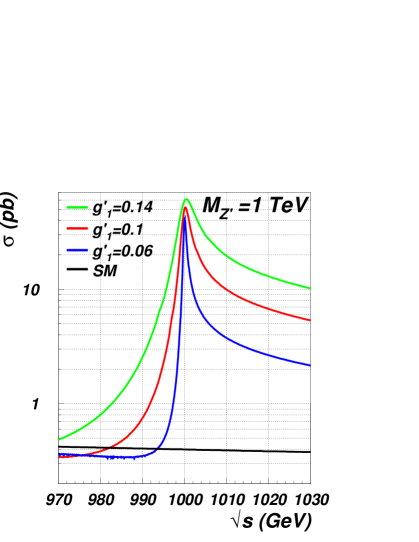
(a)

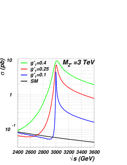
(b)

Figure 3: Cross section for the process $e^{+}e^{-}\rightarrow X\to\mu^{+}\mu^{-}$ cross section for the signal ($X=\gamma,Z,Z^{\prime}$) and the SM background ($X=\gamma,Z$) plotted against $\sqrt{s_{e^{+}e^{-}}}$ (notice here the GeV scale) at a LC, for (3a) fixed $M_{Z^{\prime}}=1$ TeV and (3b) fixed $M_{Z^{\prime}}=3$ TeV.

In these last two plots, one can neatly appreciate the effects of the ISR, implying that the maximum cross section (i.e., the one at the $Z^{\prime}$ peak) is actually achieved for LC energy values higher than the $Z^{\prime}$ mass. Notice that this energy shift is proportional to the the $Z^{\prime}$ width (i.e., the larger the stronger the $g^{\prime}_{1}$ coupling) and is an example of the radiative return mechanism, whereby ISR effectively modulates $\sqrt{s_{e^{+}e^{-}}}$ over a wide mass range (below the maximum, the machine energy itself), so that, even at a fixed LC energy, one can reconstruct the $e^{+}e^{-}\to\mu^{+}\mu^{-}$ line shape by simply plotting the di-muon invariant mass distribution, $M_{\mu\mu}$: see Fig. 4 (for an illustrative combination of $\sqrt{s_{e^{+}e^{-}}}$, $M_{Z^{\prime}}$ and $g^{\prime}_{1}$’s).

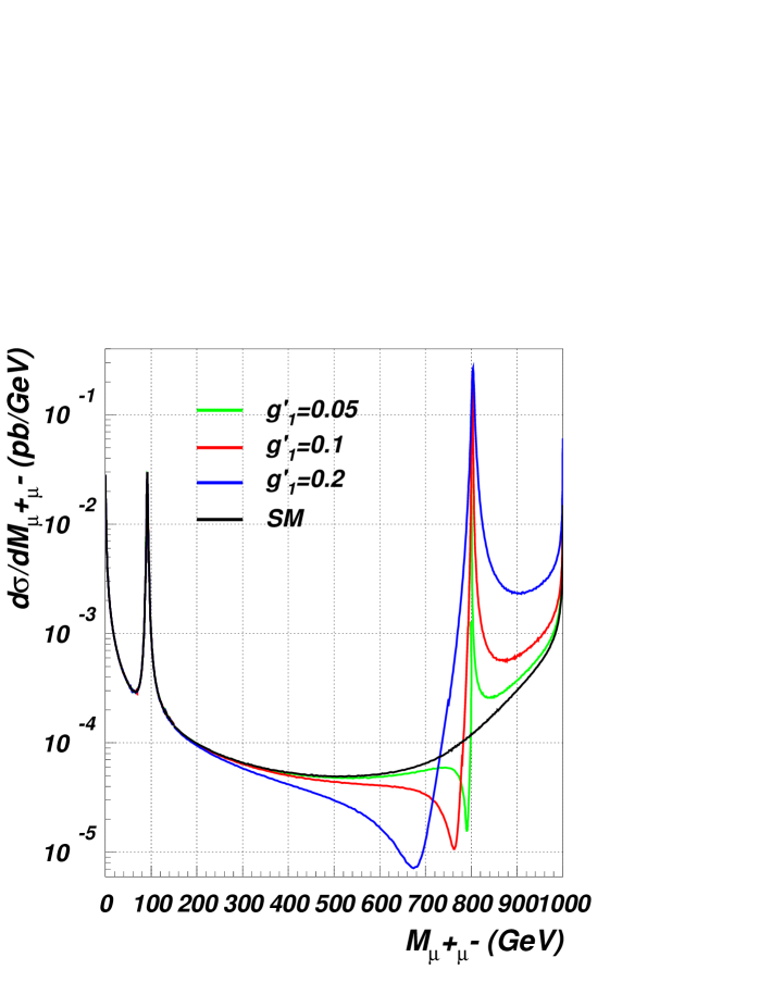
Figure 4: $\frac{d\sigma}{dM_{\mu\mu}}(e^{+}e^{-}\rightarrow\gamma,Z,Z^{\prime}\to\mu^{+}\mu^{-}$), for $\sqrt{s_{e^{+}e^{-}}}=1$ TeV, $M_{Z^{\prime}}=800$ GeV and $g_{1}^{\prime}=0.05,~{}0.1$ and $0.2$. (Notice that the latter value is shown just for sake of illustration, although already excluded by ref. [22], see eq. 15).

While the potential of future LCs in detecting $Z^{\prime}$ bosons of the $B-L$ model is well established whenever $\sqrt{s_{e^{+}e^{-}}}\geq M_{Z^{\prime}}$, we would like to remark here upon the fact that, even when $\sqrt{s_{e^{+}e^{-}}}<M_{Z^{\prime}}$, there is considerable scope to establish the presence of the additional gauge boson, through the interference effects that do arise between the $Z^{\prime}$ and SM sub-processes ($Z$ and photon exchange). Even when the $Z^{\prime}$ resonance is beyond the kinematic reach of the LC, significant deviations are nonetheless visible in the di-muon line shape of the $B-L$ scenario considered, with respect to the the SM case. This is well illustrated in Figs. 5a–5b for the case of $\sqrt{s_{e^{+}e^{-}}}$ held fixed and $M_{Z^{\prime}}$ variable (in terms of absolute rates) and in Figs. 6a–6b for the case of $M_{Z^{\prime}}$ held fixed and $\sqrt{s_{e^{+}e^{-}}}$ variable (in terms of relative rates). Notice that in the studies presented in Figs. 5a–5b we have applied a useful kinematical cut $M_{\mu\mu}>200$ GeV, aimed at eliminating the production of a SM $Z$-boson due to the radiative return mechanism as well as enhancing the aforementioned interference effects.

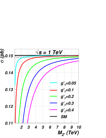
(a)

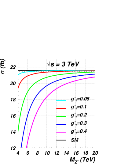
(b)

Figure 5: Cross section for the process $e^{+}e^{-}\rightarrow\gamma,Z,Z^{\prime}\to\mu^{+}\mu^{-}$ plotted against $M_{Z^{\prime}}$, for (5a) $\sqrt{s_{e^{+}e^{-}}}=1$ TeV and (5b) $\sqrt{s_{e^{+}e^{-}}}=3$ TeV. Notice that we have implemented here the cut $M_{\mu\mu}>200$ GeV. The shading corresponds to a 1% deviation from the SM hypothesis.

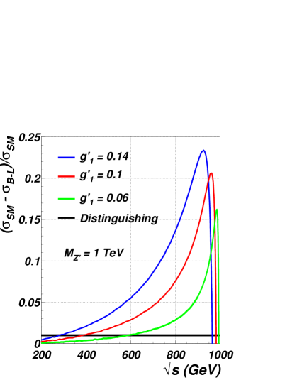
(a)

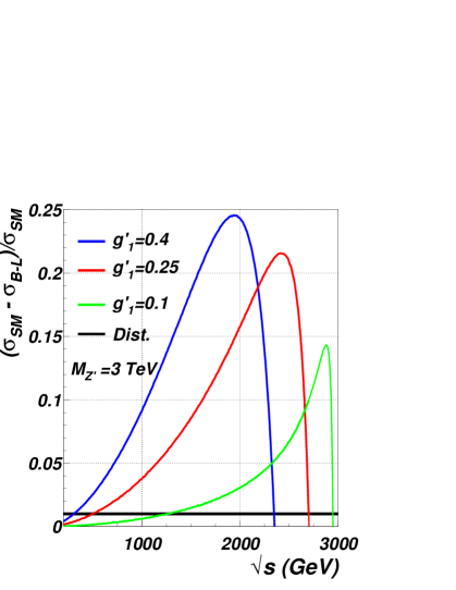
(b)

Figure 6: The relative difference for the cross section of the process $e^{+}e^{-}\rightarrow\mu^{+}\mu^{-}$ between the $B-L$ scenario and the SM plotted against $\sqrt{s_{e^{+}e^{-}}}$, for (6a) $M_{Z^{\prime}}=1$ TeV and (6b) $M_{Z^{\prime}}=3$ TeV. The horizontal line corresponds to a 1% deviation from the SM hypothesis.

Incidentally, also notice that such strong interference effects do not onset in the case of the LHC, as it can clearly be seen from Fig. 7, owing to smearing due to the PDFs.

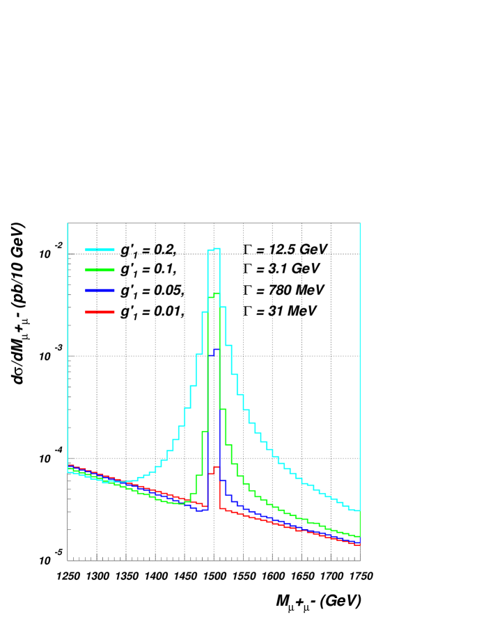
Figure 7: $\frac{d\sigma}{dM_{\mu\mu}}(pp\rightarrow\mu^{+}\mu^{-})$ in the $B-L$ model at the LHC ($\sqrt{s_{pp}}=14$ TeV), with $M_{Z^{\prime}}=1.5$ TeV, using a 10 GeV binning.

In Figs. 5a–5b and Figs. 6a–6b we have assumed and indicated a $1\%$ uncertainty band on the SM predictions (which is quite conservative). Under the assumption that SM di-muon production will be known with a 1% accuracy we would like to illustrate how the LHC $3\sigma$ observation potential of a heavy $Z^{\prime}$ (Fig. 8) is comparable to a LC indirect sensitivity to the presence of a $Z^{\prime}$, even beyond the kinematic reach of the machine. This is shown in Tab. 3, which clearly shows that a CLIC type LC will be (indirectly) sensitive to much heavier $Z^{\prime}$ bosons than the LHC. For example, for $g^{\prime}_{1}=0.1$, such a machine would be sensitive to a $Z^{\prime}$ with mass up to 10 TeV whilst the LHC can observe a $Z^{\prime}$ with mass below 4 TeV (for the same coupling). Even a LC with $\sqrt{s_{e^{+}e^{-}}}=1$ TeV (a typical ILC energy) will be indirectly sensitive to larger $M_{Z^{\prime}}$ values that the LHC, for large enough values of the $g^{\prime}$ coupling. For example, such a machine will be sensitive to a $Z^{\prime}$ with mass up to $7.5$ TeV for $g^{\prime}_{1}=0.2$ whilst the LHC would be able to observe a ${Z^{\prime}}$ only below $4.7$ TeV or so (again, for the same coupling).

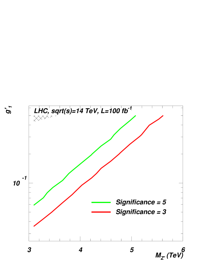
Figure 8: Significance contour levels plotted against $g_{1}^{\prime}$ and $M_{Z^{\prime}}$ at the LHC for $L=100\;{\rm fb}^{-1}$ ($\sqrt{s_{pp}}=14$ TeV, $M_{Z^{\prime}}\geq 3$ TeV). The shaded area corresponds to the region of parameter space excluded experimentally, in accordance with eq. (15).

$g_{1}^{\prime}$	$M_{Z^{\prime}}$ (TeV)
	LHC ($3\sigma$ observation)	LC ($\sqrt{s}=1$ TeV, 1% level)	LC ($\sqrt{s}=3$ TeV, $1\%$ level)
0.05	3.4	2.2	5.5
0.1	4.1	3.8	10
0.2	4.7	7.5	19.5

Table 3: Maximum $M_{Z^{\prime}}$ value accessible at the LHC and a LC for selected $g^{\prime}_{1}$ values in our $B-L$ model. At the LHC we assume $L=100\;{\rm fb}^{-1}$.

One interesting possibility opened up by such a strong dependence of the $e^{+}e^{-}\to\mu^{+}\mu^{-}$ process in the $B-L$ scenario on interferences (up to a 25% effect judging from, e.g., Fig. 6) is to see whether this potentially gives unique and direct access to measuring the $g^{\prime}_{1}$ coupling. In fact, notice that in the case of $Z^{\prime}$ studies on or near the resonance (i.e., when $\sqrt{s_{e^{+}e^{-}}}\approx M_{Z^{\prime}}$), the $B-L$ rates are strongly dependent on $\Gamma_{Z^{\prime}}$ (hence on all couplings entering any possible $Z^{\prime}$ channel, that is, not only $\mu^{+}\mu^{-}$). Instead, when $\sqrt{s_{e^{+}e^{-}}}\ll M_{Z^{\prime}}$ and $|\sqrt{s_{e^{+}e^{-}}}-M_{Z^{\prime}}|\gg\Gamma_{Z^{\prime}}$, one may expect that the role of the $Z^{\prime}$ width in such interference effects is minor, the latter being mainly driven by the strength of $g^{\prime}_{1}$. We prove this to be the case in Fig. 9, where we have artificially varied the $Z^{\prime}$ width by a factor of $10$ in each set of $M_{Z^{\prime}}$ and $g^{\prime}_{1}$ values chosen: the dashed line (corresponding to $\Gamma_{Z^{\prime}}=100$ GeV) always coincides with the solid one (corresponding to $\Gamma_{Z^{\prime}}=10$ GeV). Therefore, it is clear that the dependence on $\Gamma_{Z^{\prime}}$ is negligible (the more so the larger the difference $|\sqrt{s_{e^{+}e^{-}}}-M_{Z^{\prime}}|$) whereas the one on either $M_{Z^{\prime}}$ or $g^{\prime}_{1}$ is always significant. Hence, in presence of a known value for $M_{Z^{\prime}}$ (e.g., from a LHC analysis), one could extract $g_{1}^{\prime}$ from a fit to the line shape. In fact, the same method, to access this coupling, could be exploited at future LCs independently of LHC inputs, as interference effects of the same size also appear when $\sqrt{s_{e^{+}e^{-}}}>M_{Z^{\prime}}$: see again Fig. 4.

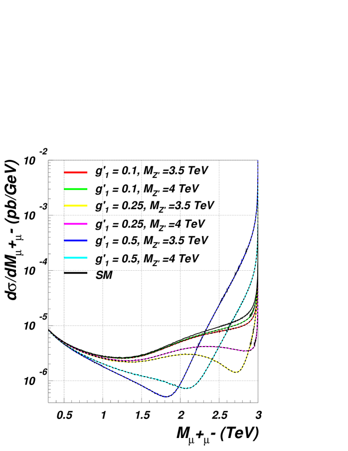
Figure 9: $\frac{d\sigma}{dM_{\mu\mu}}(e^{+}e^{-}\rightarrow\mu^{+}\mu^{-})$ in the $B-L$ model, for several combinations of $M_{Z^{\prime}}$ and $g_{1}^{\prime}$, treating $\Gamma_{Z^{\prime}}$ as an independent parameter: $10$ GeV for colored solid lines, $100$ GeV for black dashed ones. Here, $\sqrt{s_{e^{+}e^{-}}}=3$ TeV.

5 Conclusions

In summary, we have demonstrated the unique potential of future $e^{+}e^{-}$ LCs in discovering $Z^{\prime}$ bosons produced resonantly via the $e^{+}e^{-}\to\mu^{+}\mu^{-}$ process within the minimal $U(1)_{B-L}$ extension of the SM. The scope in this respect of future LCs operating in the TeV range can be well beyond the reach of the LHC, in line with what had already been assessed in the literature concerning generic $Z^{\prime}$ scenarios.

We have also presented the indirect sensitivity of LCs to a $Z^{\prime}$ below its production threshold, assuming a 1% combined uncertainty on the $e^{+}e^{-}\to\mu^{+}\mu^{-}$ production cross section. For example, for $\sqrt{s_{e^{+}e^{-}}}=1(3)$ TeV, one can access $Z^{\prime}$ masses up to 2.2(5.5) TeV for $g_{1}^{\prime}=0.05$. If the value of this coupling is four times larger, an ILC(CLIC) setup would be respectively sensitive to the range $M_{Z^{\prime}}\leq$ 10(20) TeV.

Furthermore, in either kinematic configuration (i.e, for LCs with centre-of-mass energy below or above the $Z^{\prime}$ mass), it may be possible to access both the mass and (leptonic) couplings of the $Z^{\prime}$, thereby constraining the underlying model, in parameter space regions allowed by experimental contraints (see Sect. 4.1).

These results have been obtained by exploiting parton level analyses based on exact matrix element calculations appropriately accounting for the finite width and all interference effects in the $e^{+}e^{-}\to\mu^{+}\mu^{-}$ channel. We have also taken into account beam-shtrahlung effects as well as general detector acceptance geometry. Finally, we would like to notice that, even if our model can be fully determined by a direct detection and a line shape analysis of the $Z^{\prime}$ resonance, in case of model checking or indirect observation throughout interference effects, the need of additional studies could arise. In this connection, there is further room to explore the LC potential to study $Z^{\prime}$ physics by exploiting beam polarisation and/or asymmetries in the cross section, which will be reported on separately [20].

References

- [1] W. Buchmuller, C. Greub and P. Minkowski, Phys. Lett. B 267 (1991) 395.
- [2] P. Minkowski, Phys. Lett. B 67 (1977) 421; M. Gell-Mann, P. Ramond and R. Slansky, in Supergravity, eds. P. Van Nieuwenhuizen and D. Freedman (North-Holland, Amsterdam, ), p. ; T. Yanagida, in Proceedings of the Workshop on the Unified Theory and the Baryon Number in the Universe, eds. O. Sawadaand and A. Sugamoto (KEK, Tsukuba, ), p. ; S.L. Glashow, in Quarks and Leptons, eds. M.Lèvy et al. (Plenum, New York ), p. ; R.N. Mohapatra and G. Senjanović, Phys. Rev. Lett. 44 () .
- [3] M. Fukugita and T. Yanagida, Phys. Lett. B 174 (1986) 45.
- [4] L. Basso, A. Belyaev, S. Moretti and C. H. Shepherd-Themistocleous, arXiv: 0812.4313 [hep-ph].
- [5] K. Huitu, S. Khalil, H. Okada and S.K. Rai, Phys. Rev. Lett. 101 (2008) 181802; W. Emam and S. Khalil, Eur. Phys. J. C 522 (2007) 625.
- [6] K. Abe et al., [The ACFA Linear Collider Working Group], arXiv:hep-ph/0109166; T. Abe et al., [The American Linear Collider Working Group], arXiv:hep-ex/0106055; arXiv:hep-ex/0106056; arXiv:hep-ex/0106057; arXiv:hep-ex/0106058; E. Accomando et al. [ECFA/DESY LC Physics Working Group], Phys. Rept. 299 (1998) 1; J.A. Aguilar-Saavedra et al., [The ECFA/DESY LC Physics Working Group], arXiv:hep-ph/0106315; K. Ackermann et al., preprint DESY-PROC-2004-01, DESY-04-123, DESY-04-123G.
- [7] T. G. Rizzo, In the Proceedings of 1996 DPF / DPB Summer Study on New Directions for High-Energy Physics (Snowmass 96), Snowmass, Colorado, 25 Jun - 12 Jul 1996, pp NEW136 [arXiv:hep-ph/9612440].
- [8] See, e.g.: J. Hewett and T. G. Rizzo, Phys. Rept. 183 (1989) 193 (and references therein); A. Leike, Phys. Rept. 317 (1999) 143 (and references therein); M. Cvetic and P. Langacker, hep-ph/9707451; A. Djouadi, A. Leike, T. Riemann, D. Schaile and C. Verzegnassi, Z. Phys. C 56 (1992) 289; V. Barger et al., Phys. Rev. D 33 (1986) 1912; T.G. Rizzo, Phys. Rev. D 34 (1986) 1438; F. del Aguila, E. Laermann and P.M. Zerwas, Nucl. Phys. B 297 (1988) 1; W. Buchmuller and C. Greub, Nucl. Phys. B 363 (1991) 345.
- [9] J. Brau et al. [ILC Collaboration], arXiv:0712.1950 [physics.acc-ph].
- [10] A. Pukhov, arXiv:hep-ph/0412191.
- [11] A.V. Semenov, arXiv:hep-ph/9608488.
- [12] See: http://www.ifh.de/pukhov/calchep.html.
- [13] S. Jadach and B. Ward, Comp. Phys. Commun. 56 (1990) 351; S. Jadach and M. Skrzypek, Z. Phys. C 49 (1991) 577.
- [14] J. A. Aguilar-Saavedra et al., Eur. Phys. J. C 46 (2006) 43.
- [15] G. Weiglein et al. [LHC/LC Study Group], Phys. Rept. 426 (2006) 47.
- [16] G. L. Bayatian et al. [CMS Collaboration], preprint CERN-LHCC-2006-001, CMS-TDR-008-1.
- [17] T. Behnke et al. [ILC Collaboration], arXiv:0712.2356 [physics.ins-det].
- [18] S. I. Bityukov and N. V. Krasnikov, Nucl. Instr. and Meth. A452 (2000) 518.
- [19] See: http://durpdg.dur.ac.uk/hepdata/pdf.html.
- [20] L. Basso, A. Belyaev, S. Moretti and G. M. Pruna, work in progress.
- [21] M. Carena, A. Daleo, B.A. Dobrescu and T.M.P. Tait, Phys. Rev. D 70 (2004) 093009.
- [22] G. Cacciapaglia, C. Csaki, G. Marandella and A. Strumia, Phys. Rev. D 74 (2006) 033011.
- [23] T. Aaltonen et al. [CDF Collaboration], Phys. Rev. Lett. 102, 091805 (2009)
- [24] A. Djouadi, J. Lykken, K. Monig, Y. Okada, M. J. Oreglia and S. Yamashita, arXiv:0709.1893 [hep-ph].
- [25] G. Guignard (editor) [The CLIC Study Team], preprint CERN-2000-008 (2000).