Sersic galaxy with Sersic halo models of early-type galaxies: a tool for N-body simulations

Abstract

We present spherical, non-rotating, isotropic models of early-type galaxies with stellar and dark-matter components both described by deprojected Sersic density profiles, and prove that they represent physically admissible stable systems. Using empirical correlations and recent results of N-body simulations, all the free parameters of the models are expressed as functions of one single quantity: the total (B-band) luminosity of the stellar component.

We analyze how to perform discrete N-body realizations of Sersic models. To this end, an optimal smoothing length is derived, defined as the softening parameter minimizing the error on the gravitational potential for the deprojected Sersic model. It is shown to depend on the Sersic index $n$ and on the number of particles of the N-body realization.

A software code allowing the computations of the relevant quantities of one- and two-component Sersic models is provided. Both the code and the results of the present work are primarily intended as tools to perform N-body simulations of early-type galaxies, where the structural non-homology of these systems (i.e. the variation of the shape parameter along the galaxy sequence) might be taken into account.

1. Introduction

Merging of red-sequence galaxies might be an important channel for the formation of massive early-type galaxies (ETGs). Such dry mergers have been observed to take place and have an impact on the population of ETGs at both low (up to $z\sim 0.3$; Whitaker & van Dokkum 2008, Masjedi, Hogg & Blanton 2008), and intermediate redshift, in cluster and field environments (van Dokkum et al., 1999; van Dokkum, 2005; Tran et al., 2005; Bell et al., 2006). A further evidence comes from the fact that the stellar mass on the red sequence has been found to be nearly doubled from $z\sim 1$ (Zucca et al., 2006; Bell et al., 2004) on, implying that at least some red galaxies must be formed from merging systems that are either very dusty or gas-poor (Faber et al., 2005). K-band selected samples also revealed a substantial population of old, passively evolving, massive ETGs already in place at $1<z<2$, with luminosity and stellar mass functions evolving only weakly up to $z\sim 0.8-1$ (Cimatti et al., 2002; Bundy et al., 2006; Cimatti, Daddi & Renzini, 2006).
From the theoretical viewpoint, dry mergers are also expected to play a major role. Using semi-analytical models, Khochfar & Burkert (2003) found that a large fraction of present-day ETGs are indeed formed by merging bulge-dominated systems and that the fraction of spheroidal mergers increases with luminosity, with massive ETGs being formed by nearly dissipationless events. As shown by De Lucia et al. (2006), more massive ETGs are expected to be built up of several stellar pieces, with the number of effective stellar progenitors increasing up to five for the most massive galaxies. On the other hand, hydro-dynamical simulations have also shown that accretion of smaller disk-dominated galaxies (in the mass ratio of 1:10) could also have an important role in the evolution of massive ETGs, explaining the presence of the tidal debris observed at $z\sim 0$ (Feldmann, Mayer & Carollo, 2008).

To constrain the role of dry mergers in galaxy formation, it is of importance to perform merging simulations of spheroidal systems, comparing the properties of merger remnants to observations. So far, merging simulations of ETGs have been mostly used to constrain the origin of the empirical correlations among galaxy’s observed quantities, such as the Faber-Jackson (Faber & Jackson, 1976, hereafter $FJ$), the Kormendy (Kormendy, 1977, hereafter KR), and the Fundamental Plane (Djorgovski & Davis, 1987, hereafter FP) relations. The impact of dry merging has been investigated in several works (e.g. Capelato, de Carvalho & Carlberg 1995; Dantas et al. 2003; Evstigneeva et al. 2004; Nipoti, Londrillo & Ciotti 2003). They have all agreed that dissipationless merging is able to move galaxies along the FP. But it is not clear if dry mergers are also able to preserve other observed correlations (Boylan-Kolchin, Chung-Pei & Eliot, 2006). For instance,  Nipoti, Londrillo & Ciotti (2003) found that the products of repeated merging of gas-free galaxies are characterized by an unrealistically large effective radius and a mass-independent velocity dispersion, while Evstigneeva et al. (2004) found that only the merging of massive galaxies, that lie on the KR, leads to end-products that still follow that relation.
 In previous works, merging simulations have been performed by means of ETG’s models where the stellar component is described by simple analytic density laws, such as the King or the Hernquist profiles. This approach implicitly neglects one key observational feature: the structural non-homology of the ETG population (Graham & Colless, 1997). It is well established that the observed light profiles of ETGs deviate from a pure $r^{1/4}$ law, being better described by the Sersic (1968) model (Caon, Capaccioli & D’Onofrio, 1993; D’Onofrio, Capaccioli & Caon, 1994; Graham et al., 1996). The Sersic index (shape parameter), $n$, measuring the steepness of the light profile, changes systematically along the galaxy sequence, the more luminous galaxies having higher $n$. Moreover, the shape parameter also correlates with other observed properties of ETGs, such as the effective parameters and the central velocity dispersion (Graham, 2002), as expected in view of the correlation of $n$ with the luminosity. Different values of $n$ correspond to physical systems that differ significantly in their phase-space density structure, with higher Sersic indices describing galaxies whose light profile is significantly more concentrated toward the center, with an extended low surface brightness halo. Thus, merging systems with different $n$’s might lead to a different evolution of the phase-space density of merging remnants with respect to that of “homologous” King/Hernquist models. For what concerns dark matter haloes, previous simulations have usually adopted either the Navarro-Frenk-White (NFW) profile (Navarro, Frenk & White, 1995) or the Hernquist (1990) profile. However, as shown by  Merritt et al. (2005) and  Merritt et al. (2006) (hereafter MGM06), galaxy- and cluster-sized halos are actually better described by using either the Einasto’s model (Einasto, 1968) or the Prugniel & Simien model (Prugniel & Simien, 1997) rather than a NFW-like profile (Navarro, Frenk & White, 1995). The Einasto’s model is identical in functional form to the Sersic model, but is used to describe the deprojected (rather than the projected) density profile, while the Prugniel & Simien model is an analytic approximation to the deprojected Sersic profile.  Merritt et al. (2005) (hereafter MNL05) and MGM06 found that the deprojected Sersic model (i.e. the Prugniel & Simien model) provides a better fit to the projected mass density profile of simulated dark-matter halos, with a Sersic index value of $n\sim 3$ for galaxy-sized dark-matter halos.

Hence, the deprojected Sersic model seems able to describe both the stellar and dark matter components of ETGs. Driven by that, we present here new simple models of ETGs, where both components follow the deprojected Sersic law. Hereafter, we refer to these models as double Sersic ($S^{2}$) models. The models describe spherical, non-rotating, isotropic systems, and are intended as a tool to perform N-body simulations of ETGs. In a companion contribution (Coppola et al. 2009b, in preparation), we use the $S^{2}$ models to investigate how dissipation-less (major and minor) mergers affect the structural properties of ETGs, such as the shape of their light profile and their stellar population gradients. The present paper aims at: (i) describing the main characteristics of the $S^{2}$ models, by deriving the corresponding potential-density pair and distribution function (Sec. 2), and discussing their physical consistency and stability (Sec. 3); (ii) describing how to perform discrete N-body realization of the models, by adopting an optimal gravitational smoothing length for simulation codes (Sec. 4); (iii) giving a set of recipes to fix all the free model parameters (Sec. 5); (iv) providing the software code to compute dynamical/structural properties of both the one- and two-component Sersic models. Summary and discussion are drawn in Sec. 6.

2. The double Sersic ($S^{2}$) model

2.1. The deprojected Sersic model

The surface brightness profile of ETGs, $I(R)$, is accurately described by the Sersic law (Capaccioli, Caon & D’Onofrio, 1992; Caon, Capaccioli & D’Onofrio, 1993; D’Onofrio, Capaccioli & Caon, 1994):

$$I(R;n)=I_{0}\exp\left[-b\,(R/R_{e_{L}})^{1/n}\right]\;,$$ (1)

where $I_{0}$ is the central surface brightness, $R$ is the (equivalent) projected distance to the galaxy center, $n$ is the Sersic index (shape parameter), and $b$ is a function of $n$, defined in such a way that $R_{e_{L}}$ is the effective (half-light) radius of the galaxy (Ciotti, 1991, 1999). The quantity $b$ is approximated at better than 1$\%$ by the relation $b\sim exp\left[0.6950+\ln(n)-0.1789/n\right]$ (Lima Neto, Gerbal & Márquez, 1999).

For a spherical system, under the assumption that the stellar mass-to-light ratio, ${M}_{{}_{L}}/L$, does not change with radius, the spatial mass density profile of the stellar component, $\rho_{{}_{L}}$, is obtained by solving the Abel integral equation (Binney & Tremaine 1988),

$$\rho_{{}_{L}}(r)=-\frac{1}{\pi}\frac{{M}_{{}_{L}}}{L}\int_{r}^{\infty}\frac{dI}{dR}\,\frac{dR}{\sqrt{R^{2}-r^{2}}}$$ (2)

where $r$ is the distance to the galaxy center. Setting $u=r/R$ and inserting Eq. 1 into the Abel equation, one obtains the following expression:

$$\rho_{{}_{L}}(r;n) = \rho_{0_{L}}\;\widetilde{\rho}(x;n)=$$ (3)

$$\rho_{0_{L}}\frac{b}{\pi n}x^{\frac{1}{n}-1}\int_{0}^{1}\frac{u^{-1/n}\,\exp[-bx^{1/n}u^{-1/n}]\;du}{\sqrt{1-u^{2}}},\;$$

where $x=r/R_{e_{L}}$ is the distance to the galaxy center in units of $R_{e_{L}}$, $\widetilde{\rho}(x;n)$ is the dimensionless deprojected density profile, and $\rho_{0_{L}}={M}_{{}_{L}}/R_{e_{L}}^{3}\cdot b^{2n}/(2\pi n\,\Gamma(2n))$ is the scaling factor of the stellar density profile. Here, $\Gamma$ denotes the complete gamma function, and the expression of $\rho_{0_{L}}$ is obtained by using eq. 4 of Ciotti (1999), which gives the total luminosity of the Sersic model as a function of $I_{0}$, $R_{e_{L}}$, and $n$. From Eq. 3, one obtains the mass profile:

$${M}_{{}_{L}}(r;n) = {M}_{0_{L}}\widetilde{M}(x;n)=$$ (4)

$$M_{0_{L}} \frac{4}{b^{2n}}\int_{0}^{1}\frac{u^{2}}{(1-u^{2})^{1/2}}\;\gamma\left[2n+1,b\left(\frac{x}{u}\right)^{1/n}\right]du,\;$$

where $\widetilde{M}$ is the dimensionless mass profile, and ${M}_{0_{L}}={M}_{{}_{L}}b^{2n}/(2\pi n\,\Gamma(2n))$ is the scaling factor of ${M}_{{}_{L}}(r)$. From the Laplace equation, one finds the following expression for the gravitational potential:

$$\varphi_{{}_{L}}(r;n) = \varphi_{0_{L}}\,\widetilde{\varphi}(x;n)=-\varphi_{0_{L}}\frac{{\widetilde{M}}(x;n)}{x}+$$ (5)

$$- \varphi_{0_{L}}\frac{4}{b^{n}}\int_{0}^{1}u(1-u^{2})^{-\frac{1}{2}}\gamma\left(n+1,b\left(\frac{x}{u}\right)^{\frac{1}{n}}\right)du,\;$$

where $\widetilde{\varphi}(x;n)$ is the dimensionless gravitational potential, and $\varphi_{0_{L}}={G{M}_{{}_{L}}}/{R_{e_{L}}}$ is the corresponding scaling factor. As shown in Secs. 2.2 and 2.3, the above equations provide the essential ingredients to construct the $S^{2}$ models.

We notice that, due to the existence of radial gradients in stellar population properties (such as age and metallicity) of ETGs (e.g. Peletier et al. 1990), the assumption of a constant mass-to-light ratio (${M}_{{}_{L}}/L(r)=const.$) might not actually reflect the physical properties of early-type systems. As discussed in Sec. 6, considering the observational results on age and metallicity gradients in ETGs, the ${M}_{{}_{L}}/L$ is expected to vary significantly with galaxy radius (up to $\sim 50\%$) at optical wavebands (B-band). However, the variation is significantly reduced, becoming consistent with zero within observational uncertainties, at Near-Infrared (NIR) wavebands. According to that, we implicitly assume here that the parameters $R_{e_{L}}$ and $n$, entering the normalization factors of the potential–density pair of the $S^{2}$ models, are those describing the NIR profile of ETGs. In Sec. 4, we describe how to derive the free parameters of the $S^{2}$ models according to this assumption.

The deprojection of the Sersic law has been already presented in several works (Ciotti 1991; Prugniel & Simien 1997; Mazure & Capelato 2002; Terzić & Graham 2005). Following  Mellier & Mathiez (1987),  Prugniel & Simien (1997) provided an analytical approximation to the spatial density profile of the $R^{1/n}$ model (Eq. 3). Lima Neto, Gerbal & Márquez (1999) showed that the Prugniel & Simien approximation reproduces the deprojected Sersic profile with an accuracy better than 5$\%$, in the radial range of $10^{-2}$ to $10^{3}R_{e_{L}}$, for Sersic indices between $n\sim 0.5$ and $n\sim 10$. The Prugniel & Simien model has been also adopted by Terzić & Graham (2005) to present one-component Sersic models of ETGs with power-law cores. Exact solutions to the deprojection of the $R^{1/n}$ model have been provided by Mazure & Capelato (2002), in terms of the so-called Meijer G functions, while Ciotti (1991) presented exact numerical expressions for the mass, gravitational potential, and central velocity dispersion of the one-component Sersic model. In the present work, we report a concise reference to the integral equations that define the density-potential pair, the mass profile and the distribution function of the deprojected Sersic law. All the quantities characterizing the Sersic model can be numerically computed by using a set of publicly available Fortran programs (see App. A).

2.2. The dark matter Sersic model

MNL05 and MGM06 found that the deprojected Sersic law provides a better fit to the density profile of dark matter halos than the NFW law. MNL05 found that a Sersic index value of $n=3.00\pm 0.17$ is required to fit the profile of galaxy-sized halos. On the other hand, MGM06 fitted the Prugniel & Simien model to the density profiles of galaxy-sized halos, finding a best-fitting value of $n\sim 3.59\pm 0.65$. Considering the lower uncertainty of the MNL05 estimate, we describe the dark matter component of the models with a deprojected Sersic model having $n=3$. The corresponding density-potential pair and mass profile are then obtained from the equations:

$$\rho_{{}_{D}}(r) = \frac{\mu}{x_{{}_{D}}^{3}}\;\rho_{0_{L}}\;\widetilde{\rho}\left(\frac{x}{x_{{}_{D}}};n=3\right)$$ (6)

$${M}_{{}_{D}}(r) = \mu\;{M}_{0_{L}}\;\widetilde{M}\left(\frac{x}{x_{{}_{D}}};n=3\right)$$ (7)

$$\varphi_{{}_{D}}(r) = \frac{\mu}{x_{{}_{D}}}\;\varphi_{0_{L}}\;\widetilde{\varphi}\left(\frac{x}{x_{{}_{D}}};n=3\right),$$ (8)

where the dimensionless density-potential pair ($\widetilde{\rho}$, $\widetilde{\varphi}$) and the dimensionless mass profile $\widetilde{M}$ are obtained by setting $n=3$ in Eqs. 3, 4 and 5, respectively. Here, we have denoted as $\mu={{M}_{{}_{D}}}/{{M}_{{}_{L}}}$ the ratio of the total halo mass, ${M}_{{}_{D}}$, to the total stellar mass ${M}_{{}_{L}}$, and $x_{{}_{D}}={R_{e_{D}}}/{R_{e_{L}}}$ the ratio of the (projected) effective radii of the dark matter and stellar components.

We notice that although we fix here the shape parameter value of the dark-matter component, the $S^{2}$ models could be directly generalized to the case where the Sersic index of the halo component changes with its mass . Such a dependece is somewhat suggested by the results of MNL05 and MGM06, who found that cluster-sized halos ($M_{{}_{D}}\sim 10^{15}M_{\odot}$) are better described with Sersic index values of $2.38\pm 0.25$ and $\sim 2.89\pm 0.49$, respectively, these values being systematically smaller than those obtained for galaxy-sized halos. However, one should notice that, when fitting dwarf-sized dark matter halos ($M_{{}_{D}}\sim 10^{10}M_{\odot}$), MNL05 found a best-fitting Sersic index value of $3.11\pm 0.05$, which is fully consistent with that of $3.00\pm 0.17$ found for galaxy-sized halos ($M_{{}_{D}}\sim 10^{12}M_{\odot}$). Hence, current results seem to suggest a very similar Sersic index value of $\sim 3$ for galaxy-sized halos of different masses, supporting our assumption of a fixed $n$ value.

2.3. Density-potential pair and Distribution Function

The total mass density profile is obtained by adding up the profiles of the stellar and dark matter components:

$$\rho(r)=\rho_{{}_{L}}\!+\!\rho_{{}_{D}}=\rho_{0_{L}}\left[\;\widetilde{\rho}(x;n)+\frac{\mu}{x_{{}_{D}}^{3}}\;\widetilde{\rho}\left(\frac{x}{x_{{}_{D}}};3\right)\right].$$ (9)

From the linearity of the Laplace equation, the total gravitational potential is equal to $\varphi(r)=\varphi_{{}_{L}}\!+\!\varphi_{{}_{D}}$, where $\varphi_{{}_{L}}$ and $\varphi_{{}_{D}}$ are obtained from Eqs. 5 and 8. A similar expression can also be obtained for the mass profile, combining Eqs. 4 and 7. We note that the global density-potential pair and the mass profile are completely defined from five parameters, which are the dimensional quantities ${M}_{{}_{L}}$ and $R_{e_{L}}$, and the dimension-less parameters $x_{{}_{D}}$, $\mu$, and $n$.

The distribution function of a stationary, spherical, isotropic system depends only on the binding energy $E$ and is uniquely defined by the density-potential pair through the Eddington formula  (Binney & Tremaine 1988):

$$f(\mathcal{E})=\frac{1}{\sqrt{8}\pi^{2}}\left[\int_{0}^{\mathcal{E}}\frac{d^{2}\rho}{d\Psi^{2}}\frac{d\Psi}{\sqrt{\mathcal{E}-\Psi}}+\frac{1}{\sqrt{\mathcal{E}}}\left(\frac{d\rho}{d\Psi}\right)_{\Psi=0}\right]\;,$$ (10)

where $\Psi(r)\equiv-\varphi(r)+\varphi_{0}$ and $\mathcal{E}\equiv-E+\varphi_{0}$ is the relative binding energy, with $\varphi_{0}$ being a suitably defined constant (see Binney & Tremaine, 1988). For the $S^{2}$ models, the global potential and density profiles are proportional to the dimensional factors $\varphi_{0_{L}}$ (see Eqs. 5 and 8) and $\rho_{0_{L}}$ (see Eqs. 3 and 6). Hence, using Eq. B1 in App. B, one finds that, unless of a scaling factor depending on $M_{{}_{L}}$ and $R_{e_{L}}$, the $f(\mathcal{E})$ is determined by the three dimension-less parameters $x_{{}_{D}}$, $\mu$, and $n$. As for the case of single Sersic models (Ciotti, 1991), one can show that the second term on the right side of Eq. 10 is always equal to zero for all possible values of $x_{{}_{D}}$, $\mu$, and $n$. In fact, one can write $(d\rho/d\Psi)_{\Psi=0}=\lim_{r\rightarrow\infty}(d\rho/dr)(dr/d\Psi)$. For $r\rightarrow\infty$, the first derivative of the gravitational potential decreases as $r^{-2}$, while the first derivative of the density decreases exponentially (see eq. 8 of Ciotti 1991), implying that $\lim_{r\rightarrow\infty}(d\rho/dr)(dr/d\Psi)=0$. In App. B, we report in detail how to calculate the distribution function by expressing the function $\frac{d^{2}\rho}{d\Psi^{2}}$ in terms of the first and second derivatives of $\widetilde{\rho}$, the gravitational potential $\widetilde{\varphi}$, and the mass profile of the dark matter and stellar components.

3. Physical consistency and stability

The Eddington inversion does not guarantee that the distribution function is a physically admissible stationary solution of the Boltzmann equation. To this effect, for a given density-potential pair, one has to show that $f(\mathcal{E})$ is non-negative for all positive values of the relative binding energy. As shown by Ciotti (1991), one-component spherical, non-rotating, isotropic Sersic models are always physically admissible, while in the anisotropic case, a minimum anisotropy radius exists for the model to be admissible, with this radius depending on the Sersic index $n$ (Ciotti & Lanzoni, 1997).

The distribution function of the $S^{2}$ models is computed by numerical integration of the Eddington formula, as described in App. B. Fig. 1 plots the $f(\mathcal{E})$ for different values of the free parameters $n$, $\mu$ and $x_{{}_{D}}$. The value of $\mu$ is varied in the range of zero – no dark matter halo – to a value of $10^{6}$, where the stellar component is negligible and the system is completely dark matter dominated. We consider values of $x_{{}_{D}}$ from $0.1$ to $10^{2}$, corresponding to the two extreme cases where the dark matter component is either more concentrated or significantly more extended than the luminous one. For all combinations of $x_{{}_{D}}$ and $\mu$, different values of $n$ are plotted. We find that for positive values of the relative binding energy the condition $f(\mathcal{E})\geq 0$ is always fulfilled, implying that the $S^{2}$ models are physically admissible.

To analyze the stability of the two-component Sersic models, following Ciotti (1991), we study the sign of the first derivative of the distribution function. According to Antonov’s theorem (see Binney & Tremaine, 1988, pag. 306), if $\frac{df}{d\varepsilon}\geq 0$, the system is stable against both radial and non-radial perturbations. As shown in App. B, a necessary condition for $\frac{df}{d\varepsilon}\geq 0$ is given by:

$$g(r;n,\mu,x_{{}_{D}})=-\left[\frac{d^{2}\rho}{dr^{2}}\left(\frac{d\Psi}{dr}\right)-\frac{d\rho}{dr}\frac{d^{2}\Psi}{dr^{2}}\right]\geq 0\,.$$ (11)

For the two-component Sersic models, $g(r)$ is derived numerically as described in App. B. Fig. 2 plots $g(r)$ as a function of $r$ for the same sets of $n$, $\mu$, and $x_{{}_{D}}$ values as in Fig. 1. The condition $g(r)\geq 0$ is always verified, proving the stability of $S^{2}$ models.

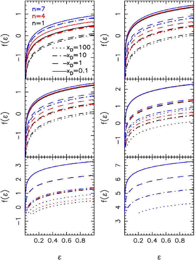
Figure 1.— Physical consistency of the $S^{2}$ models. The logarithm of the distribution function $f$ is plotted as a function of the relative binding energy $\mathcal{E}$. The panels correspond to different values of the halo to stellar mass ratio, $\mu$. From left to right and top to bottom, the panels correspond to $\mu=0,0.1,1,10,10^{2},10{{}^{6}}$. For each plot, as shown in the upper-left panel, curves with different colors correspond to different values of the Sersic index, while different line types denote different values of the ratio, $x_{{}_{D}}$, between the effective radii of the halo and stellar components. The $f(\varepsilon)$ has been computed by adopting natural units, where $M_{{}_{L}}=1$, $R_{e_{L}}=1$, and the gravitational constant was set to one.

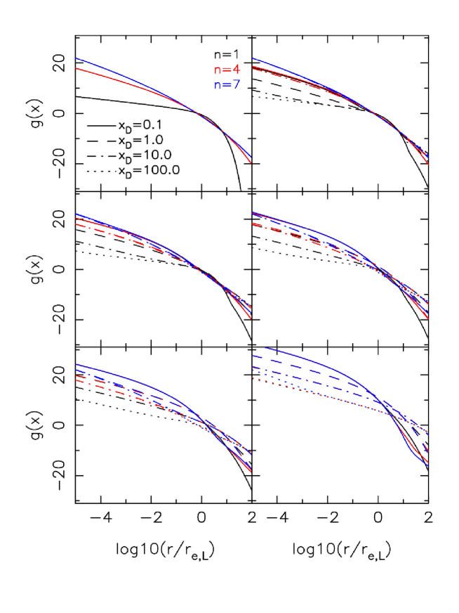
Figure 2.— Stability of the $S^{2}$ models. The logarithm of the quantity $g(r)$ (see Eq. 11) is plotted as a function of the logarithm of the dimensionless radius $r/r_{e,{L}}$. Colors and line types are the same as in Fig. 1. From left to right and top to bottom, the panels correspond to $\mu=0,0.1,1,10,10^{2},10{{}^{6}}$. Natural units have been adopted as for Fig. 1.

4. Physical scales

There are five free parameters that completely characterize the $S^{2}$ model, i.e. the mass of the stellar component, ${M}_{{}_{L}}$, its effective radius, $R_{e_{L}}$, the Sersic index of the stellar component, $n$, the mass of the dark matter halo, ${M}_{{}_{D}}$, and the corresponding effective radius, $R_{e_{D}}$. Alternatively, one can use the dimensional quantities, ${M}_{{}_{L}}$ and $R_{e_{L}}$, and the dimension-less parameters $x_{{}_{D}}$, $\mu$, and $n$ defined in Sec. 2.2. Here, we describe some recipes to express all the free parameters as a function of one single quantity, the absolute luminosity of the stellar component. This procedure is intended as an handy tool to use the $S^{2}$ models in merging simulations of ETGs. We refer to absolute magnitudes in the B band, $M_{B}$, since most of the relations we use in the following are expressed in that band. In the following, magnitudes are expressed with respect to the Vega system.

The quantity $R_{e_{L}}$ is related to the total luminosity by the Kormendy relation (Kormendy, 1977; Capaccioli, Caon & D’Onofrio, 1992):

$$\log R_{e_{L,B}}=\alpha\langle\!\mu\!\rangle_{e}+\beta\;.$$ (12)

where $R_{e_{L,B}}$ is the galaxy effective radius in the B-band and $\langle\!\mu\!\rangle_{e}$ is the mean effective surface brigthness inside $R_{e_{L,B}}$. Expressing $R_{e_{L,B}}$ in units of kpc, one has

$$\langle\!\mu\!\rangle_{e}=-5\log(R_{e_{L}})-M_{B}+25+2.5\log(6^{8}/(2\pi)).$$ (13)

As discovered by Capaccioli, Caon & D’Onofrio (1992) and Graham & Guzmán (2003), ETGs follow two different trends in the $R_{e}$–$\langle\!\mu\!\rangle_{e}$ plane, according to their luminosity. The separation between the two families of bright and ordinary ellipticals occurs between $M_{B}=-19$ and $M_{B}=-20$. We adopt here a separation value of $-20$. By a linear fit of the data in figure 9 of Graham & Guzmán (2003), we obtain $\alpha\sim 0.35$ and $\beta\sim-6.75$ for the bright galaxies ($M_{B}<-20$) and $\alpha=-0.02$ and $\beta=0.45$ for the ordinary ellipticals ($M_{B}>-20$). The latter value of $\alpha$ is consistent with that of $0.34\pm 0.01$ found by La Barbera et al. (2003b), who showed that the Kormendy relation of bright ETGs does not change significantly with redshift up to redshift $z\sim 0.6$ and that the intrisic scatter of the relation amount to $0.4\pm 0.03$ in $\langle\!\mu\!\rangle_{e}$ (i.e. $\sim 0.14$ dex in $R_{e_{L,B}}$). In order to derive the Near-Infrared effective radius $R_{e_{L}}$, we use Eq. 12 to compute $R_{e_{L,B}}$ from $M_{B}$, and then transform $R_{e_{L,B}}$ into $R_{e_{L}}$. To this aim, we consider that ETGs have on average a radial color gradient of about $-0.2$ in $B-K$, and that their internal color gradients are observed not to change significantly with galaxy luminosity (see Peletier, Valentijn, & Jameson 1990; Peletier et al. 1990). Following Sparks & Jörgensen (1993), the above value of the color gradient implies that the effective radius of ETGs decreases by $\sim 20\%$ from $B$ to $K$ band. Thus, we derive $R_{e_{L}}$ from the relation

$$R_{e_{L}}=0.8R_{e_{L,B}}\;.$$ (14)

The Sersic parameter, $n$, of the stellar component depends on luminosity through the magnitude-Sersic index relation (Caon, Capaccioli & D’Onofrio, 1993). Trujillo et al. (2004) presented this relation for a sample of $200$ ellipticals at redshift $z\sim 0$. A linear fit to the data in their figure 1 gives 

$$\log n_{B}=-0.1219\cdot M_{B}-1.6829,$$ (15)

where $n_{B}$ is the Sersic index of ETGs in the B-band. The Sersic index is not expected to change significantly from optical to NIR wavebands. For instance, as found by La Barbera et al. (2008), ETGs have on average $\log(n_{r}/n_{K})=-0.007\pm 0.009$, where $n_{r}$ and $n_{K}$ denote the r- and K-band Sersic indices. Hence, we set $n=n_{B}$, and use Eq. 15 to derive also the NIR Sersic index of the stellar component.

To express $R_{e_{D}}$ as a function of $M_{B}$, we use the finding that dark matter halos follow a relation between the half–mass radius, $R_{e_{D}}$, and the average projected surface mass-density inside that radius, $\langle\mu\rangle_{e_{D}}$, similar to the Kormendy relation of galaxies (Graham et al. 2006; hereafter GMM06). This result was obtained from GMM06 for a sample of galaxy-sized dark-matter halos as massive as $10^{12}M_{\odot}$. We note that GMM06 derived the quantities $R_{e_{D}}$ and $\langle\mu\rangle_{e_{D}}$ by fitting the projected halo density profile with the Prugniel-Simien model (Prugniel & Simien, 1997), i.e. the same kind of profile as adopted here for the dark matter component of the $S^{2}$ models . We write

$$\log R_{e_{D}}=\delta\cdot\langle\mu\rangle_{e_{D}}+\zeta.$$ (16)

For systems more massive than $10^{10}$ $M_{\odot}$, GMM06 report a slope of $\delta\sim 1/3$. This mass range corresponds to $\log R_{e_{D}}>0.4$ (see fig. 1b of GMM06). Performing a linear fit to the data in figure 2a of GMM06, we obtain $\zeta\sim 10/3$, with $R_{e_{D}}$ being expressed in units of kpc.

Then, we derive the mass of the dark-matter and stellar components as a function of the B-band magnitude, using the recent results obtained from Cappellari et al. (2006) (hereafter CAP06) for elliptical and lenticular galaxies in the SAURON project (Bacon et al., 2001). From the relation between dynamical mass-to-light ratio in $I-$band and total mass of CAP06 (see their eq. 9), one obtains:

$${M}_{e_{L}}+{M}_{e_{D}}=1.175\cdot 10^{0.1317-0.528\cdot M_{B}}\;.$$ (17)

where ${M}_{e_{L}}$ and ${M}_{e_{D}}$ denote the masses of the stellar and dark matter components within $R_{e_{L}}$. This relation provides the total dynamical mass with an accuracy of $\sim 30\%$. Following Fukugita, Shimasaku & Ichikawa (1995), we derive Eq. 17 by assuming a typical $B\!-\!I$ color term  for elliptical galaxies of $2.23$ and the B- and I-band magnitudes of the Sun to be $5.51$ and $4.08$, respectively. Under the assumption of a radially constant $M_{{}_{L}}/L$ ratio, one has ${M}_{{}_{L}}=2{M}_{e_{L}}$. According to CAP06, ${M}_{e_{L}}$ is about $0.16$dex smaller  than the dynamical mass within $R_{e_{L}}$, i.e. ${M}_{e_{L}}\sim 0.6918\left({M}_{e_{L}}+{M}_{e_{D}}\right)$. Thus, from Eq. 17, one obtains:

$${M}_{e_{L}}=0.81286\cdot 10^{0.1317-0.528\cdot M_{B}}\;,$$ (18)

and

$${M}_{e_{D}}=0.36214\cdot 10^{0.1317-0.528\cdot M_{B}}\;.$$ (19)

In order to relate ${M}_{e_{D}}$ to ${M}_{{}_{D}}$, we use the analytic expression for the projected luminosity profile of the Sersic model (see eq. 2 of Ciotti 1999). Since the dark-matter component is described by a Sersic model having $n=3$, we can write:

$$M_{e_{D}}=M_{{}_{D}}\cdot\gamma\left(6,b_{3}\cdot\left(\frac{R_{e_{L}}}{R_{e_{D}}}\right)^{1/3}\right)$$ (20)

where $\gamma$ denotes the normalized incomplete gamma function , and $b_{3}=5.6631$. The quantity $b_{3}$ is computed by setting $n=3$ in the analytic approximation of $b$ reported in Sec. 2.1. From Eqs. 18 and Eq. 19, one obtains:

$$M_{{}_{D}}=\frac{0.36214\cdot 10^{0.1317-0.528\cdot M_{B}}}{\gamma\left(6,b_{3}\cdot\left(\frac{R_{e_{L}}}{R_{e_{D}}}\right)^{1/3}\right)}\;.$$ (21)

In practice, for a given $M_{B}$, $R_{e_{L}}$ is computed from Eqs. 12 and 14, and the quantities $R_{e_{D}}$ and $M_{{}_{D}}$ are derived by solving simultaneouly Eqs. 21 and 16. This is equivalent to solve the non-linear equation

$$7.1077+\frac{\zeta}{2.5\delta}+0.528M_{B}+\log\left[\gamma\left(6,b_{3}\cdot\left(\frac{R_{e_{L}}}{R_{e_{D}}}\right)^{1/3}\right)\right]+\frac{5\delta-1}{2.5\delta}\log(R_{e_{D}})=0$$ (22)

with respect to $R_{e_{D}}$. We denote the first member of this equation as $\theta(R_{e_{D}})$. As an example, Fig. 3 plots $\theta(R_{e_{D}})$ as a function of $R_{e_{D}}$, for the case $M_{B}=-21$. The figure shows that Eq. 22 has in general two distinct solutions, corresponding to the points where the horizontal dashed line in the figure crosses the curve. One has a small-halo solution with $R_{e_{D}}<R_{e_{L}}$ (and $M_{e_{D}}<M_{e_{L}}$), and a large-halo case, whereby the dark-matter component is larger and more massive than the stellar one. In the small-halo case, the $M_{e_{D}}$ value is four (eight) times smaller than $M_{e_{L}}$ for $M_{B}=-22$ ($-20$), while $R_{e_{D}}$ is three (ten) times smaller than $R_{e_{L}}$. This would imply that almost all the dark matter in ETGs should be enclosed within one $R_{e_{L}}$, in disagreement with dynamical, X-Ray, and weak lensing studies (Matsushita et al., 1998; Wilson et al., 2001; Gerhard et al., 2001). Therefore, we consider here only the large-halo solutions of Eq. 22. We notice that Eq. 16 applies to the case of massive galaxy-sized halos ($M_{{}_{D}}\sim 10^{12}$), which might be appropriate only for bright galaxies ($M_{B}<-20$). For galaxies fainter than $M_{B}=-20$, we fix  the ratio of dark to stellar effective radius to the value obtained for $M_{B}=-20$ and then derive the total dark-matter mass from Eq. 21.

Figure 3.— Derivation of the effective radius of the dark matter component for a galaxy with $M_{B}=-21$. The $R_{e_{D}}$ is derived by solving the equation $\theta(R_{e_{D}})=0$ (Eq. 22). The horizontal dashed line marks the value of $\theta(R_{e_{D}})=0$, while the vertical dashed line shows the effective radius $R_{e_{L}}$ of the stellar component. The points of intersection between the horizontal line and the curve denote the values of $R_{e_{D}}$ which are consistent with our procedure. We consider only the large-halo solution (right part of the plot), with $R_{e_{D}}\!>\!R_{e_{L}}$ (see the text).

To summarize, we use the Kormendy and the luminosity–Sersic index relations to express $R_{e_{L}}$ and $n$ as a function of $M_{B}$. Then, by using Eq. 18 and solving Eq. 22, we also express ${M}_{{}_{D}}$, $R_{e_{D}}$, and ${M}_{{}_{L}}$ as a function of $M_{B}$. In Tab. 1, as an example, we show the values of the five free parameters of the $S^{2}$ models that are obtained from the above procedure in six cases equally spanning the magnitude range of $-22$ to $-17$. In general, the procedure leads to have galaxy models where the dark matter component is less massive and less extended in lower luminosity systems. On the other hand, the relative amount of dark matter within $R_{e_{L}}$ does not depend on galaxy luminosity, in agreement with the finding of CAP06 (see Eqs. 18 and 19 above).

We remark that the above procedure derives the free parameters of the $S^{2}$ models by using the observed properties of early-type systems at $z\sim 0$. Hence, one possible caveat when applying the above procedure to merging simulations is that such properties might not necessarly be the same for the high-redshift progenitors of ETGs. Moreover, one should consider that most of the observed relations (such as the Kormendy and the luminosity-size relations) of ETGs have significant intrinsic dispersion (see the values reported above), implying a dispersion, at a given magnitude, also in the parameter’s values reported in Tab. 1.

$M_{{}_{B}}$	${M}_{{}_{L}}$	$R_{e_{L}}$	${M}_{{}_{D}}$	$R_{e_{D}}$	$n$	${M}_{e_{D}}$
	($10^{10}$ $M_{\odot}$)	(kpc)	($10^{10}$ $M_{\odot}$)	(kpc)		$(10^{10}$ $M_{\odot}$)
(1)	(2)	(3)	(4)	(5)	(6)	(7)
-22	90.94	14.84	267.20	108.60	10.0	20.25
-21	26.96	5.07	199.74	75.50	7.5	6.00
-20	7.99	1.73	133.26	45.50	5.7	1.78
-19	2.37	0.90	39.53	23.79	4.3	0.53
-18	0.70	0.87	11.72	22.81	3.2	0.16
-17	0.21	0.83	3.47	21.88	2.5	0.05

Table 1Derivation of the free parameters of the double Sersic models as a function of luminosity. The columns are: (1) $B-$band magnitude, $M_{B}$, of the stellar component, (2) total stellar mass, ${M}_{{}_{L}}$, (3) effective radius of the stellar component, $R_{e_{L}}$, (4) total mass of the dark matter halo, ${M}_{{}_{D}}$, (5) effective radius of the dark matter component, $R_{e_{D}}$, (6) Sersic index $n$, and (7) mass of the dark matter halo within $R_{e_{L}}$.

5. Optimal softening length

Performing discrete realizations of galaxy models requires that a given gravitational softening parameter, $\epsilon$, is adopted. The value of $\epsilon$ should depend on the number of particles, $N$, defining the mass and spatial resolution of the simulation. Here, we discuss how to set $\epsilon$ and $N$ for the Sersic models.

5.1. The optimal smoothing length

Usually, the value of $\epsilon$ is chosen with some ad hoc prescription. One fixes the total number of particles in the simulation (which is limited from the available CPU resources) and then assigns the $\epsilon$ in order to achieve the desired spatial resolution. Merritt (1996) (hereafter MER96) showed that the softening length of an N-body system can be chosen in an objective (optimum) way by minimizing the average error in the gravitational force computation over the whole space. Following a similar approach, we assign $\epsilon$ by minimizing the average error in the computation of the gravitational potential. We consider here the spline softening kernel of Monaghan & Lattanzio (1985), which is implemented into the simulation code Gadget-2 (Springel, 2005). Hereafter, we express $\epsilon$ in units of the effective radius, $R_{e_{L}}$.
We start by considering the case of single Sersic models. For a given Sersic index, $n$, and a given number of particles, $N$, we generate several realizations of the deprojected Sersic model. For a given realization, we calculate the softened gravitational potential at the position of each particle and the corresponding true gravitational potential (Eq. 5). Then, the rms of the relative absolute differences between the softened and true potential, $\Delta\phi/\phi$, is computed over all the particles. We average the value of $\Delta\phi/\phi$ over 100 realizations. Fig. 4 shows how the mean value of $\Delta\phi/\phi$ changes as a function of $\epsilon$. As example, the figure plots the case of a de Vaucouleurs model ($n=4$) for two different values of $N$.

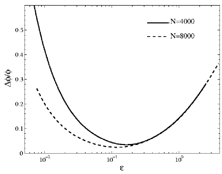
Figure 4.— Mean value of the relative error on the gravitational potential as a function of the softenin length, $\epsilon$, for a Sersic model with $n=4$. As shown in the upper-right corner of the plot, the dashed and solid curves correspond to discrete realizations with a different number of particles, $N$.

In both cases, there is a minimum in $\Delta\phi/\phi$. Following an argument similar to that of MER96, the existence of a minimum can be explained as follows. For low $\epsilon$, the error is dominated by the differences between the point-like Newtonian potential of each particle and the true gravitational potential. Increasing $\epsilon$, these differences become smaller and $\Delta\phi/\phi$ decreases. For large $\epsilon$, the discrete potential is smoothed on a scale larger than the typical interparticle separation  and the discrete potential is overly smoothed with respect to the true gravitational potential. Increasing $\epsilon$, this large-scale smoothing becomes more and more important, and the value of $\Delta\phi/\phi$ increases as well. For a given number of particles, we define the position of the minimum as the optimal smoothing length, $\epsilon_{o}$. Increasing the number of particles, the typical interparticle separation, $d_{N}$, decreases, and thus the optimal smoothing is obtained for smaller $\epsilon$. Fig. 5 plots $\epsilon_{o}$ as a function of $N$ for different values of the Sersic index. The optimal softening length turns out to decrease as either $n$ or $N$ increase. This is due to the fact that, in both cases, the typical particle separation, $d_{N}$, decreases. In particular, when $n$ increases, the mass profile of the model is more concentrated in the center and, at fixed $N$, $d_{N}$ is smaller. As shown in Fig. 5, the trend of $\epsilon_{o}$ vs. $N$ can be accurately modeled by a power law, $\epsilon_{o}=\beta N^{-\alpha}$, where both $\alpha$ and $\beta$ depend on the value of $n$. The value of $\alpha$ changes from $\sim 0.28$ for $n=1$ to $\sim 0.54$ for $n=7$. For $n\leq 2$, the shape of the Sersic profile is flatter than for higher values of $n$, and the $\epsilon_{o}$ is essentially proportional to the mean interparticle separation, with $\epsilon_{o}\propto N^{-1/3}$. For a de Vaucouleurs profile ($n=4$), the value of $\alpha$ is $\sim 0.4$, in agreement with that of $0.44$ found by MER96 for the Hernquist model. For higher $n$, the Sersic profile becomes more and more peaked in the center and the value of $\alpha$ deviates more and more from the simple $\alpha\sim 1/3$ expectation. Fig. 6 shows how the mean relative error on the potential, $\Delta\phi/\phi$, depends on the number of particles and the Sersic index when adopting the optimal smoothing parameter. For a given Sersic model, the error decreases with $N$ following the power-law $\Delta\phi/\phi\propto N^{-1/2}$, in agreement with what found by MER96 for the Hernquist model. For a given $N$, the error is larger for higher Sersic index. Hence, if a given accuracy in the computation of the gravitational potential has to be achieved, for higher $n$ a larger number of particles has to be adopted.

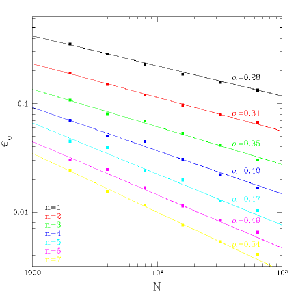
Figure 5.— Dependence of the optimal softening length of one-component models, $\epsilon_{0}$, on the number of particles, $N$, for different values of the Sersic index, $n$. Different colors correspond to different values of $n$ as shown in the lower-left corner of the plot. Solid lines plot the best-fitted power laws to the trends of $\epsilon_{o}$ vs. $N$ (see the text). The exponent $\alpha$ of each fitted power-law is reported on the top–right of the corresponding line.

Figure 6.— The relative error on the gravitational potential, $\Delta\phi/\phi$, is plotted as a function of the number of particles, $N$, for three one-component Sersic models having $n=1$ (dashed line), $n=4$ (solid line) and $n=7$ (dotted line), respectively. The gray line shows the power-law fit, $\Delta\phi/\phi\propto N^{-1/2}$, to the points for $n=4$.

5.2. Models in isolation

To perform discrete realizations of the $S^{2}$ models, one can adopt different softening lengths for the stellar and dark matter components, according to the optimal definition given above. However, these softening parameters represent an optimal choice only for one-component Sersic models, and we are not guaranteed that they provide also an accurate choice for the two-component models. To verify that the optimal prescription for $\epsilon$ gives sensible results even in the case of two-component models, we compared the evolution of double and single Sersic models in isolation. As example, we consider here (1) a one-component model with ${M}_{{}_{L}}\sim 27\cdot 10^{10}$ $M_{\odot}$ and $R_{e_{L}}\sim 5$ kpc, and (2) an $S^{2}$ model whose parameters are the same as those reported in Tab. 1 for the case $M_{B}=-21$. Model (1) is obtained by considering only the stellar component of model (2). To evolve the models in isolation, we adopt $50000$ particles of luminous matter in both cases and $75000$ particles of dark matter for model (2). Looking at Fig. 6, we see that adopting the optimal smoothing parameter for these values of $N$ allows an accuracy better than $10\%$ on the gravitational potential to be achieved. The simulations were ran over $5$ Gyrs with the simulation code Gadget-2, using a Beowulf system with thirty-two AMD-Opteron 244 processors. As initial conditions, we created discrete realizations of the models by computing their density profile and distribution function with the set of Fortran codes that are made publicly available (see App. A). The softening parameters were chosen according to Fig. 5. For the stellar component, we adopt $\epsilon_{o}=0.013$ kpc, while for the dark matter component we set $\epsilon_{o}=0.053$ kpc.
Fig. 7 (upper panel) plots the relative absolute variation of the total energy of both systems, $|\Delta E/E_{0}|$, as a function of time, where $E_{0}$ is the total initial energy of the simulation. Apart from a small and slow secular drift, one can see that for both models the total energy of the system is preserved, with a value of $|\Delta E/E_{0}|$ smaller than $\sim 8\%$ after $5$ Gyrs. Fig. 7 (lower panel) also shows the evolution of the virial ratio, $|2T/W|$, where $T$ and $W$ are the total kinetic and potential energy of the system, as a function of time. For both the single and $S^{2}$ models, the deviations from the virial equilibrium, $2T/W=1$, are small, amounting to at most $\sim 0.7\%$ in modulus after $5$ Gyrs.

Figure 7.— Variations in total energy and virial ratio as a function of time. Triangles and circles correspond to one- and two-component models, respectively (see the text). Notice that the deviations from conservation of total energy ($|\Delta E/E_{0}|=0$) and the virial equilibrium ($|2T/W|=1$) are small for both models.

Fig. 8 plots, for the one-component model, the radial profiles in mass, velocity dispersion, and anisotropy at $T=0$ Gyrs (left panels), and the relative variations of these profiles after the model has been evolved for $5$ Gyrs (right panels). The profiles are plotted in a radial range of $r_{min}=3\epsilon_{o}$ to $r_{max}=5R_{e_{L}}$. The value of $r_{min}$ is chosen in order to avoid the inner region of the model which is affected by the smoothing in the gravitational potential. The maximum radius, $r_{max}$, is set to a sensible value where one can compare the model to the observed profiles of ETGs. The simulation shows that the profile in mass is preserved within a few percentages over the whole radial extent. The velocity dispersion and the anisotropy profile are also preserved within $\sim 10\%$. Fig. 9 plots the same profiles as in Fig. 8 for the stellar component of model (2). Remarkably, all the profiles are preserved even in this case within $\sim 10\%$ over at least $5$ Gyrs. The same result was obtained when considering the properties of the dark-matter component of model (2), and for all the $S^{2}$ models whose parameters are listed in Tab. 1.

Figure 8.— Evolution in mass, velocity dispersion, and anisotropy profiles of single Sersic models. We plot the case of the model (1) described in the text. Left panels plot the mass (top), velocity dispersion (middle) and anisotropy (bottom) profiles of the model at $T=0$ Gyr. The right panels show the relative absolute radial variation of the profiles after $T=5$ Gyrs. For each value of the spatial radius $r$, the variation is computed with respect to the initial value at that radius. We note that the variations from $|2T/W|=1$ are small for both models.

Figure 9.— Same as Fig. 8 for the luminous component of $S^{2}$ models. The case of model (2) is shown (see the text).

6. Summary and Discussion

We have presented models of ETGs consisting of a stellar component and a dark matter halo that follow the deprojected Sersic law. The models describe non-rotating, isotropic, spherical systems, whose density–potential pair is derived under the assumption that the stellar mass-to-light ($M_{{}_{L}}/L$) ratio of galaxies does not depend on radius.

As mentioned in Sec. 2.1, the constant $M_{{}_{L}}/L$ assumption might not reflect the real physical properties of ETGs. Galaxies are observed to have internal color gradients, reflecting variations of stellar population properties (such as age and metallicity) from the galaxy center to the outskirts (e.g. Peletier, Valentijn, & Jameson 1990). It has been shown that (i) color gradients are mainly driven by a mean metallicity gradient in the range of $\nabla_{Z}=-0.2$ to $\nabla_{Z}=-0.3$, with an uncertainty of $\sim 0.1$; and that (ii) a small positive age gradient of $\nabla_{t}\sim 0.1$ is also consistent with observations (see e.g. Peletier et al. 1990; Saglia et al. 2000; Idiart, Michard & de Freitas Pacheco 2002; La Barbera et al. 2003a; Tamura & Ohta 2003). Here, we denote as $\nabla_{Z}$ and $\nabla_{t}$ the logarithmic variations of metallicity and age per decade in galaxy radius. From the theoretical viewpoint, age gradients are expected to arise in the formation of ETGs by gas-rich mergers, where early-type remnants are better described by a two-component stellar profile, with the two components having different ages (Hopkins, Cox, & Hernquist, 2008). We can use the above values of $\nabla_{Z}$ and $\nabla_{t}$ to infer the corresponding radial variations of $M_{{}_{L}}/L$. Using single stellar populations models from Bruzual & Charlot (2003) with a Scalo IMF and an age of $12$Gyr , one obtains that a metallicity gradient of $\nabla_{Z}=-0.2$ ($-0.3$) corresponds to a variation of $34\%$ ($51\%$) in the B-band $M_{{}_{L}}/L$ per decade of galaxy radius. This variation largely decreases in K-band, where the inferred variation of $M_{{}_{L}}/L$ amounts to $\sim 15\%$ ($24\%)$. Considering a positive age gradient of $0.1$dex, the $M_{{}_{L}}/L$ variation would further decrease to about $7\%$ ($10\%$) in K-band, while the above uncertainty on color gradients would translate to an error of about one third in the estimated $M_{{}_{L}}/L$ percentages. We conclude that, provided one adopts the K-band light profile of ETGs to infer the underlying distribution of stellar matter, the assumption of a constant $M_{{}_{L}}/L$ is empirically well motivated.

For what concerns the other assumptions underlying the $S^{2}$ models, one should notice that ETGs actually span a wider range of kinematical and structural properties than that considered here. For instance, the $S^{2}$ models populate the origin of the anisotropy ($v/\sigma$ vs. ellipticity) diagram, while ETGs populate different regions of it. In order to explore the corresponding effect on dry-merging simulations, some studies have realized merging simulations where the progenitors are obtained by either dissipationless (Naab, Khochfar, & Burkert, 2006) or dissipational (Cox et al., 2006; Robertson et al., 2006) merging of disk systems. This re-merger approach has the main advantage that progenitors span a wide range of ETG properties, such as $v/\sigma$, ellipticty, and isophotal shape. Though neglecting these aspects, the $S^{2}$ models have the main advantage of allowing one to explore a key observational feature: the wide range of profile shapes observed in early-type systems (Caon, Capaccioli & D’Onofrio, 1993). Moreover, re-merging of $S^{2}$ would likely allow one to further enlarge the range of kinematic and isophotal properties of merging progenitors.

The free parameters of the two components of $S^{2}$ models are assigned in order to match the observed properties of ETGs as well as recent results of N-body simulations of galaxy-sized dark matter halos. We report a concise reference to the basic integral equations that define the density-potential pair and the distribution function of the deprojected Sersic law, showing how these equations can be used to define the $S^{2}$ models. We show that for all possible values of the free parameters of the models, the total distribution function is always non-negative defined, implying that the models are physically admissible solutions of the collisionless Boltzmann equation. Moreover, the first derivative of the total distribution function is always non-negative defined, implying that the models are stable against radial and non-radial perturbations. For a given Sersic model, we present an objective prescription to adopt an optimal smoothing length of discrete model realizations. The optimal smoothing length is defined as the softening parameter that minimizes the error on the gravitational potential of the system, and depends on the Sersic index $n$ as well as on the number of particles of the simulation. The power-law relations that describe these trends are reported, with the aim of providing a prescription to create discrete realizations of $S^{2}$ systems, whose discrete gravitational potential closely matches the true model potential. As a caveat, when using such a prescription for merging simulations, one should notice that the optimal smoothing length for the progenitors might not necessarely concide with the optimal softening for the merging remnants, depending on the structural properties (i.e. the Sersic index) of the merging end-products. This issue can be addresses by exploring the effect of changing the number of particle, and the corresponding smoothing length, of the colliding systems.

We provide the Fortran code that allows one to calculate all the properties of single and double Sersic models. The code together with the recipes for computing the optimal softening scale are intended as general tools to perform merging simulations of early-type galaxies, whereby the structural non-homology of these systems (i.e. the variation of the shape parameter along the galaxy sequence) might be taken into account. In a companion contribution (Coppola et al. 2009b, in preparation), we use the $S^{2}$ models to investigate how dissipation-less (major and minor) mergers affect the structural properties of ETGs, such as the shape of their light profile and their stellar population gradients.

Appendix A Fortran codes

The properties of both the single and double Sersic models are computed by a set of FORTRAN routines. All the Fortran codes are made publicly available . For the one-component models, the code allows the user to calculate the density, mass, and gravitational potential profiles (by a numerical integration of Eqs. 3, 4, and 5), as well as the distribution function (App. B). Other quantities, such as the total potential and gravitational energy of the system, its spatial and projected velocity dispersion profiles, are also computed by specific Fortran routines. For the double Sersic model, since the computation of the density-potential pair is time-demanding, we proceed as follows.

• For a given value of the Sersic index $n$, that characterizes the luminous component of the model, we calculate the dimension-less mass, density, potential and the first and second derivatives of the density profile over a grid in the dimension-less spatial radius $x$. The same computation is done for the Sersic index of the dark matter component, $n=3$ (Sec. 2.3).

• The total density-potential pair and the distribution function are then obtained by interpolating the above radial profiles. To this effect, the values of the parameters $\mu$ and $x_{{D}}$ of the model have to be provided (Sec. 2.3).

The software to perform this interpolation procedure is also provided.

Appendix B Distribution function of the double Sersic model

In order to apply the Eddington inversion (Eq. 10), one has to calculate the function $\frac{d^{2}\rho}{d\Psi^{2}}$, where $\rho$ is the spatial density profile and $\Psi\equiv-\varphi+\varphi_{0}$ is the rescaled gravitational potential (see Sec. 2.3). We start from the following identity:

$$\frac{d^{2}\rho}{d\Psi^{2}} = \frac{d^{2}\rho}{dr^{2}}\left(\frac{d\Psi}{dr}\right)^{-2}-\frac{d\rho}{dr}\left(\frac{d\Psi}{dr}\right)^{-3}\frac{d^{2}\Psi}{dr^{2}}.$$ (B1)

Then, using the fact that $\rho(r)=\rho_{{}_{L}}+\rho_{{}_{D}}$ and $\varphi(r)=\varphi_{{}_{L}}+\varphi_{{}_{D}}$, one obtains the following expression:

$$\left[\frac{d^{2}\rho}{dr^{2}}\left(\frac{d\varphi}{dr}\right)-\left(\frac{d\rho}{dr}\right)\frac{d^{2}\varphi}{dr^{2}}\right]=\left[\frac{d^{2}\rho_{{}_{D}}}{dr^{2}}\frac{d\varphi_{{}_{D}}}{dr}-\frac{d\rho_{{}_{D}}}{dr}\frac{d^{2}\varphi_{{}_{D}}}{dr^{2}}\right]+$$

$$\left[\frac{d^{2}\rho_{{}_{L}}}{dr^{2}}\frac{d\varphi_{{}_{L}}}{dr}-\frac{d\rho_{{}_{L}}}{dr}\frac{d^{2}\varphi_{{}_{L}}}{dr^{2}}\right]-\left[\frac{d\rho_{{}_{L}}}{dr}\frac{d^{2}\varphi_{{}_{D}}}{dr^{2}}-\frac{d\rho_{{}_{D}}}{dr}\frac{d^{2}\varphi_{{}_{L}}}{dr^{2}}\right]\;.$$ (B2)

The first and second derivatives of $\rho_{{}_{L}}$ and $\rho_{{}_{D}}$ can be derived by numerically differentiating Eqs. 3 and 6. The derivatives of the gravitational potential and the density profile can be obtained from the expression of the gravitational potential and the mass profile of the stellar and dark matter components, using the following identities:

$$\frac{d\varphi_{{}_{L}}}{dr}=\frac{G{M}_{{}_{L}}}{R_{e_{L}}^{2}}\frac{\widetilde{M}(x)}{x^{2}}|_{x=r/R_{e_{L}}}\;,$$ (B3)

$$\frac{d\varphi_{{}_{D}}}{dr}=\frac{G{M}_{{}_{L}}}{R_{e_{L}}^{2}}\frac{\mu}{x_{{}_{D}}^{2}}\frac{\widetilde{M}(x/x_{{}_{D}})}{(x/x_{{}_{D}})^{2}}|_{x=r/R_{e_{L}}}\;,$$ (B4)

$$\frac{d^{2}\varphi_{{}_{L}}}{dr^{2}}=4\pi G\frac{{M}_{{}_{L}}}{R_{e_{L}}^{3}}\frac{b^{2n}}{2\pi n\Gamma(2n)}\widetilde{\varphi}_{{}_{L}}(x)-\frac{2}{R_{e_{L}}}\frac{1}{x}\frac{d\varphi_{{}_{L}}}{dr}\;,$$ (B5)

$$\frac{d^{2}\varphi_{{}_{D}}}{dr^{2}}=G\frac{{M}_{{}_{L}}}{R_{e_{L}}^{3}}\frac{\mu}{x_{{}_{D}}^{3}}\left[\frac{2b^{2m}}{m\Gamma(2m)}\widetilde{\varphi}_{D}(x/x_{{}_{D}})-\frac{2M(x/x_{{}_{D}})}{(x/x_{{}_{D}})^{3}}\right]\;,$$ (B6)

$$\frac{d\rho_{{}_{L}}}{dr}=\frac{{M}_{{}_{L}}}{R_{e_{L}}^{4}}\frac{b^{2n}}{2\pi n\Gamma(2n)}\frac{d\widetilde{\rho}}{dx}|_{x=r/R_{e_{L}}}\;,$$ (B7)

$$\frac{d\rho_{{}_{D}}}{dr}=\frac{{M}_{{}_{L}}}{R_{e_{L}}^{4}}\frac{\mu}{x_{{}_{D}}^{4}}\frac{b^{2m}}{2\pi m\Gamma(2m)}\frac{d\widetilde{\rho}}{dx}|_{x=x/x_{{}_{D}}}\;,$$ (B8)

$$\frac{d^{2}\rho_{{}_{L}}}{dr^{2}}=\frac{{M}_{{}_{L}}}{R_{e_{L}}^{5}}\frac{b^{2n}}{2\pi n\Gamma(2n)}\frac{d^{2}\widetilde{\rho}}{dx^{2}}|_{x=r/R_{e_{L}}}$$ (B9)

and

$$\frac{d^{2}\rho_{{}_{D}}}{dr^{2}}=\frac{{M}_{{}_{L}}}{R_{e_{L}}^{5}}\frac{\mu}{x_{{}_{D}}^{5}}\frac{b^{2m}}{2\pi m\Gamma(2m)}\frac{d^{2}\widetilde{\rho}}{dx^{2}}|_{x=x/x_{{}_{D}}}\;,$$ (B10)

These equations show that the $f(\mathcal{E})$ is completely defined by the first and second derivatives of the density profile, the gravitational potential and the mass profiles of the two Sersic components. In order to calculate $f(\mathcal{E})$, we derive numerically the functions $\widetilde{\rho}$, $\frac{d\widetilde{\rho}}{dr}$, $\frac{d^{2}\widetilde{\rho}}{dr^{2}}$, $\widetilde{\phi}$, and $\widetilde{M}$, and then, using Eq. B, we evaluate Eq. 10.

To prove the stability of the double Sersic models, one has to prove the condition $\frac{df}{d\varepsilon}\geq 0$ (see Sec. 3). From the Eddington formula, a necessary condition is $\frac{d^{2}\rho}{d\Psi^{2}}\geq 0$. From Eq. B1, this condition can be written as

$$\frac{d^{2}\rho}{dr^{2}}\left(\frac{d\Psi}{dr}\right)^{-2}-\frac{d\rho}{dr}\left(\frac{d\Psi}{dr}\right)^{-3}\cdot\frac{d^{2}\Psi}{dr^{2}} = \left(\frac{d\Psi}{dr}\right)^{-3}\left[\frac{d^{2}\rho}{dr^{2}}\left(\frac{d\Psi}{dr}\right)-\left(\frac{d\rho}{dr}\right)\frac{d^{2}\Psi}{dr^{2}}\right]\geq 0\;.$$ (B11)

Since $\frac{d\Psi}{dr}$ is negative (i.e. the gravitational potential is a monotonically increasing function of $r$), the previous condition is equivalent to :

$$g(r;n,\mu,x_{{}_{D}})=-\left[\frac{d^{2}\rho}{dr^{2}}\left(\frac{d\Psi}{dr}\right)-\left(\frac{d\rho}{dr}\right)\frac{d^{2}\Psi}{dr^{2}}\right]\geq 0\;,$$ (B12)

as stated in Sec. 2.3.

References

- Bacon et al. (2001) Bacon, R., et al. 2001, MNRAS, 326, 23
- Bell et al. (2004) Bell, E. F., et al. 2004, ApJ, 608, 752
- Bell et al. (2006) Bell, E. F., et al. 2006, ApJ, 640, 241
- Binney & Tremaine (1988) Binney, J., & Tremaine, S. 1987, Galactic Dynamics, Princeton University Press, Chicago
- Boylan-Kolchin, Chung-Pei & Eliot (2006) Boylan-Kolchin, M., Chung-Pei, M., & Eliot, Q. 2006, MNRAS, 369, 1081
- Bruzual & Charlot (2003) Bruzual, G., & Charlot, S. 2003, MNRAS, 344, 1000 (BC03)
- Bundy et al. (2006) Bundy, K., et al. 2006, ApJ, 651, 120
- Caon, Capaccioli & D’Onofrio (1993) Caon, N., Capaccioli, M., & D’Onofrio, M. 1993, MNRAS, 265, 1013
- Capaccioli, Caon & D’Onofrio (1992) Capaccioli, M., Caon, N., & D’Onofrio, M. 1992, MNRAS, 259, 323
- Capelato, de Carvalho & Carlberg (1995) Capelato, H. V., de Carvalho, R. R., & Carlberg, R. G. 1995, ApJ, 451, 525
- Cappellari et al. (2006) Cappellari, M., et al. 2006, MNRAS, 366, 1126
- Cimatti et al. (2002) Cimatti, A., et al. 2002, A&A, 381, L68
- Cimatti, Daddi & Renzini (2006) Cimatti, A., Daddi, E., & Renzini, A. 2006, A&A, 453, 29
- Ciotti (1991) Ciotti, L. 1991, A&A, 249, 99
- Ciotti & Lanzoni (1997) Ciotti, L., & Lanzoni, B. 1997, A&A, 321, 724
- Ciotti (1999) Ciotti, L. 1999, ApJ, 520, 574
- Ciotti, Lanzoni & Volonteri (2007) Ciotti, L., Lanzoni, B., & Volonteri, M. 2007, ApJ, 658, 65
- Cox et al. (2006) Cox, T.J., et al. 2006, ApJ, 650, 791
- Dantas et al. (2003) Dantas, C. C., et al. 2003, MNRAS, 340, 398
- De Lucia et al. (2006) De Lucia, G., et al. 2006, MNRAS, 366, 499
- de Vaucouleurs (1948) de Vaucouleurs, G. 1948, Annales d’Astrophysique, 11, 247
- Djorgovski & Davis (1987) Djorgovski, S., & Davis, M. 1987, ApJ, 313, 59
- D’Onofrio, Capaccioli & Caon (1994) D’Onofrio, M., Capaccioli, M., & Caon, N. 1994, MNRAS, 271, 523
- Einasto (1968) Einasto, J. 1968, Publications of the Tartuskoj Astrofizica Observatory, 36, 396
- Evstigneeva et al. (2004) Evstigneeva, E. A., et al. 2004, MNRAS, 349, 1052
- Faber & Jackson (1976) Faber, S. M., & Jackson, R. E. 1976, ApJ, 204, 668
- Faber et al. (2005) Faber, S. M., et al 2005, Bulletin of the American Astronomical Society, 37, 1298
- Feldmann, Mayer & Carollo (2008) Feldmann, R., Mayer, L., & Carollo, C.M. 2008, ApJ684, 1062
- Fukugita, Shimasaku & Ichikawa (1995) Fukugita, M., Shimasaku, K., & Ichikawa, T. 1995, PASP, 107, 945
- Gerhard et al. (2001) Gerhard, O., et al. 2001, AJ, 121, 1936
- Graham et al. (1996) Graham, A., et al. 1996, ApJ, 465, 534
- Graham & Colless (1997) Graham, A., & Colless, M. 1997, MNRAS, 287, 221
- Graham (2002) Graham, A. W. 2002, MNRAS, 334, 859
- Graham & Guzmán (2003) Graham, A. W., & Guzmán, R. 2003, AJ, 125, 2936
- Graham et al. (2006) Graham, A. W.,et al. 2006, AJ, 132, 2711
- Hernquist (1990) Hernquist, L. 1990, ApJ, 356, 359
- Hopkins, Cox, & Hernquist (2008) Hopkins, P. F., Cox, T. J., & Hernquist, L. 2008, ApJ, 679, 156
- Idiart, Michard & de Freitas Pacheco (2002) Idiart, T.P., Michard, R., & de Freitas Pacheco, J.A. 2002, å, 383, 30
- Khochfar & Burkert (2003) Khochfar, S., & Burkert, A. 2003, ApJ, 597, L117
- King (1962) King, I. 1962, AJ, 67, 471
- Kormendy (1977) Kormendy, J. 1977, ApJ, 218, 333
- La Barbera et al. (2003a) La Barbera, F., et al. 2003, å, 409, 21
- La Barbera et al. (2003b) La Barbera, F., et al. 2003, ApJ, 595, 127
- La Barbera et al. (2008) La Barbera, F., et al. 2008, ApJ, 689, 913
- Lima Neto, Gerbal & Márquez (1999) Lima Neto, G.B, Gerbal, D., & Márquez, I. 1999, MNRAS, 309, 481
- Masjedi, Hogg & Blanton (2008) Masjedi, M., Hogg, D. W., & Blanton, M. R. 2008, ApJ, 679, 260
- Matsushita et al. (1998) Matsushita, K., et al. 1998, ApJ, 499, 13
- Mazure & Capelato (2002) Mazure, A., & Capelato, H. V. 2002, A&A, 383, 384
- Mellier & Mathiez (1987) Mellier, Y., & Mathez, G. 1987, å, 175, 1
- Merritt (1996) Merritt, D. 1996, AJ, 111, 2462 (MER96)
- Merritt et al. (2005) Merritt, D., et al. 2005, AJ, 624, L85 (MNL05)
- Merritt et al. (2006) Merritt, D., et al. 2006, AJ, 132, 2685
- Monaghan & Lattanzio (1985) Monaghan, J.J., & Lattanzio, J.C., 1985, å, 149, 135
- Navarro, Frenk & White (1995) Navarro, J. F., Frenk, C. S., & White, S. D. M. 1995, MNRAS, 275, 56
- Naab, Khochfar, & Burkert (2006) Naab, T., Khochfar, S., & Burkert, A. 2006, ApJ, 636, 81
- Nipoti, Londrillo & Ciotti (2003) Nipoti, C., Londrillo, P., & Ciotti, L. 2003, MNRAS, 342, 501
- Peletier et al. (1990) Peletier, R. F., et al. 1990, AJ, 100, 1091 (PDI90)
- Peletier, Valentijn, & Jameson (1990) Peletier, R. F., Valentijn, E.A., and Jameson, R.F. 1990, å, 233, 62
- Prugniel & Simien (1997) Prugniel, P., & Simien, F. 1997, A&A, 321, 111
- Robertson et al. (2006) Robertson, B. et al. 2006, ApJ, 645, 986
- Saglia et al. (2000) Saglia, R.P., et al. 2000, å, 360, 911
- Scodeggio (2001) Scodeggio, M. 2001, AJ, 121, 2413
- Sersic (1968) Sersic, J. L. 1968, Cordoba, Argentina: Observatorio Astronomico, 1968,
- Sparks & Jörgensen (1993) Sparks, W.B., & Jörgensen, I. 1993, AJ, 105, 5
- Springel (2005) Springel, V., 2005, MNRAS, 364, 1105
- Tamura & Ohta (2003) Tamura, N., & Ohta, K., 2003, AJ, 126, 596
- Terzić & Graham (2005) Terzic, B., & Graham, A.W. 2005, MNRAS, 362, 197
- Tran et al. (2005) Tran, K.-V. H.,et al. 2005, ApJ, 627, L25
- Trujillo et al. (2004) Trujillo, I., Burkert, A., & Bell, E. F. 2004, ApJ, 600, L39
- van Dokkum et al. (1999) van Dokkum, P. G., et al. 1999, ApJ, 520, L95
- van Dokkum (2005) van Dokkum, P. G. 2005, AJ, 130, 2647
- Visvanathan & Sandage (1977) Visvanathan, N., & Sandage, A. 1977, ApJ, 216, 214
- Whitaker & van Dokkum (2008) Whitaker, K. E., & van Dokkum, P. G. 2008, ApJ, 676, L105
- Wilson et al. (2001) Wilson, G., et al. 2001, ApJ, 555, 572
- Zucca et al. (2006) Zucca, E., et al. 2006, A&A, 455, 879