Constant entropy sampling and release waves of shock compressions

Abstract

We present or recall several equilibrium methods that allow to compute isentropic processes, either during the compression or the release of the material. These methods are applied to compute the isentropic release of a shocked monoatomic liquid at high pressure and temperature. Moreover, equilibrium results of isentropic release are compared to the direct nonequilibrium simulation of the same process. We show that due to the viscosity of the liquid but also to nonequilibrium effects, the release of the system is not strictly isentropic.

I Introduction

The exploration of the thermodynamic behavior of materials under extreme conditions usually follows two paths corresponding to two experimental devices: isothermal compressions and shock compressions. Isothermal compressions are performed with diamond anvil cell (DAC) techniques, and are used to compress materials up to very high pressures, although with limited temperatures. On the other hand, shock compression experiments investigate the high-pressure/high temperature regions through the propagation of dynamic shock waves in the system. Nevertheless, the thermodynamic domain available using shock experiments remains limited to the so-called Hugoniot curve, which is, by definition, the collection of thermodynamic states which can be reached from a system at fixed initial conditions, with shocks of increasing strengths. Such a constraint arises from the fact that the system is assumed to satisfy Euler’s fluid equations (i.e inviscid Navier-Stokes equations), and physically meaningful shocks therefore have to fulfill the Rankine-Hugoniot conditions, which relate the thermodynamic parameters of the fluid at rest, and the thermodynamic parameters of the shocked material. Another constraint is that shock waves are adiabatic, therefore leading to very large temperature increases in the material, which limits its compressibility. The equations of state (EOS) used to predict the material’s behavior at the extreme conditions encountered are often simple extrapolations of EOS fitted on available data, i.e. shock data and DAC data. It then appeared interesting to enlarge the experimental domain of investigation of materials behavior using dynamic compression set-ups, and particularly isentropic compressions. Several experimental set-ups allow to load a pressure ramp in a material. The first one is the high pulsed power (of which the sandia Z machine and the High Explosive Pulsed PowerTasker et al. (2003, 2005) at LANL are good examples). The second one consists in using an impactor with a varying density along one direction, as proposed initially at the AIP - SWCM conference.Lyzenga and Ahrens (1981) A successful technique is to stack slices of different materials, leading to the so-called PILLOW impactors at Sandia,Barker (1983) MIVAR impactors in France,Perez (1988) and more recently the FGM (Functionaly Graded Materials) impactors at LLNL,Nguyen et al. (2006) allowing a real design of a thermodynamic path as a succession of shock and release waves. The last one concerns experiments of Barnes’ type where the compression is the consequence of the isentropic release of another material, as for example detonation products.Barnes et al. (1974); Tsypkin et al. (1975)

Experiments involving isentropic compression are of great interest to reach high compression states, or in geophysic applications to reach states representative of the earth’s core. Experiments involving a precise evaluation of release waves in materials need also general numerical methods to compute the states reached by isentropic pocesses.

Up to now, simulations involving shock processes are rather well developed due to the simplicity of the Hugoniot equations. Those studies are performed within the framework of statistical physics, see Refs. Frenkel and Smit, 2002; Allen and Tildesley, 1987 for reference textbooks on molecular simulation, and Ref. Holian and Lomdahl, 1998 for reference works on nonequilibrium simulation of shock waves. Any state lying on the Hugoniot can be reached from the reference state by searching for a given compression the temperature for which the pressure and the total energy of the system satisfies the Hugoniot relation. The search can be implemented in very efficient manners.Maillet et al. (2000); Maillet and Stoltz (2009); Bourasseau et al. (2007) Those methods are now adapted to classical molecular dynamics and Monte Carlo, as well as quantum molecular dynamics.Bernard and Maillet (2002)

Such an easy method does not exist for isentropic processes. In this paper, we present or recall several equilibrium methods which allow to follow isentropic paths, both for classical or quantum molecular dynamics simulations. We contrast these methods in terms of their precisions, rigor and computational requirements. We compare the results obtained from equilibrium simulations with release waves observed in nonequilibrium molecular dynamics. The comparison between equilibrium and nonequilibrium methods therefore measures how isentropic the expansion of the system is. It is expected that release waves of a perfect non-viscous fluid are isentropic. For simple monoatomic fluids such as argon, it is often assumed that the release is isentropic, and viscosity effects are neglected. Our results show that even in this simple case, the release is not strictly isentropic and some corrections have to be taken into account. As a by-product of our study, we also explore more precisely the relationship between the Hugoniot and the isentrope curves, from a numercial viewpoint, but also giving a statistical physics proof of the coincidence of the curves for small compressions (see Appendix B).

Organization of the paper

The paper is organized as follows. In Section II, we present the nonequilibrium method used to simulate rarefaction waves, while some equilibrium methods for constant entropy sampling are recalled in Section III - details of the practical implementaion of the thermodynamic integration and precisions on the isentropic integration are given in Appendix A and C respectively). In Section IV, a comparison of numerical results obtained in the case of release waves in argon is performed, and we discuss whether release waves are isentropic.

II Nonequilibrium simulations

II.1 Microscopic description of physical systems

We first recall how a system is described at the microscopic level using statistical mechanics.Balian (2007) Statistical physics is a theory which allows to compute thermodynamic (macroscopic) properties of a system knowing the microscopic interactions between its constitutive elements.

Consider a microscopic system composed of $N$ particles, confined in a simulation box $\mathcal{D}=[0,L_{x}]\times[0,L_{y}]\times[0,L_{z}]$. The volume of the domain is denoted by $V=|\mathcal{D}|=L_{x}L_{y}L_{z}$. The system is characterized by the positions $q=(q_{1},\dots,q_{N})$ and momenta $p=(p_{1},\dots,p_{N})$ of the particles, which have masses $m_{i}$, and interact through a potential energy function $U$. The phase-space $\Omega$ is the collection of all possible microscopic configurations $(q,p)$ of the system.

The central quantity describing the system is the Hamiltonian

$$H(q,p)=\sum_{i=1}^{N}\frac{p_{i}^{2}}{2m_{i}}+U(q_{1},\dots,q_{N}),$$ (1)

which gives the energy of a given microscopic configuration $(q,p)$. Average thermodynamic properties of the system can be computed as averages of functions of the microscopic variables $O(q,p)$ (the so-called observables) with respect to the canonical measure at a temperature $T$, for a given simulation box:

$$\mathcal{O}=\langle O\rangle_{V,T}=\int_{\Omega}O(q,p)\,\pi_{V,T}(q,p)\,dq\,dp.$$ (2)

The canonical measure associated with the Hamiltonian (1) weights microscopic states according to their energies using a Boltzmann weight:Balian (2007)

$$\pi_{V,T}(q,p)=\frac{1}{Z_{V,T}}\textrm{e}^{-\beta H(q,p)},\qquad\beta^{-1}=k_{\rm B}T,$$ (3)

where $k_{\rm B}$ is the Boltzmann constant, and the partition function $Z_{V,T}$ is a normalization factor so that (3) is indeed a probability measure:

$$Z_{V,T}=\int_{\Omega}\textrm{e}^{-\beta H(q,p)}\,dq\,dp.$$ (4)

We have indicated explicitly the dependence of the canonical measure (3) and the partition function (4) on the temperature $T$ and the volume $V$ since these will be the parameters allowed to vary in the sequel.

II.2 Nonequilibrium simulation of release waves

Similarly to what has been proposed for the simulation of shock waves,Holian and Lomdahl (1998) isentropic compressions or releases can be simulated directly using Non-Equilibrium Molecular Dynamics (NEMD). A straightforward numerical set-up to this end is simply to throw a low speed piston towards the sample (creating a weak shock), and then accelerating the piston in time. Except this external forcing, the system evolves according to the standard hamiltonian dynamics

$$\left\{\begin{array}[]{ccl}\dot{q}_{i}&=&\displaystyle\frac{p_{i}}{m_{i}},\\[10.0pt] \dot{p}_{i}&=&\displaystyle-\nabla_{q_{i}}U(q),\end{array}\right.$$ (5)

which is integrated in time with the Verlet scheme.Verlet (1967) A linear compression ramp would be obtained in the case where the acceleration is constant in time.

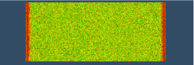
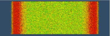
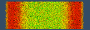
To obtain release waves, a shock wave can be loaded in a sample; when this shock wave is reflected when interacting with a free surface, it transforms into a release wave, supposedly isentropic. In this study, we start the release from an equilibrated state obtained from a preliminary canonical simulation, using three dimensional periodic boundary conditions. When the system is equilibrated, the periodic boundary conditions are removed in the $x$ direction. Two release waves are then created at the two free surfaces, and they propagate in opposite directions towards the center of the box. This process is illustrated in Figure 1.

From the simulation data presented in Figure 1, profiles of thermodynamic quantities (average densities, (kinetic) temperatures and pressures) can be extracted and averaged over thin slices. Moreover, the two release waves being symmetric, their related profiles can be averaged. A superposition of the profiles, taken at different times but projected back in the same thermodynamic diagram, is then obtained and averaged over, leading to a single profile.

The accuracy of the computation increases with the system size: an increase in the size of the transverse directions decreases the uncertainties on the slice averages (thanks to a thermodynamic limit), and an increase in the longitudinal direction allows to accumulate more profiles in time, therefore reducing statistical errors.

III Equilibrium methods for constant entropy sampling

We present in this section three methods to compute the collection of all states (in terms of their temperature, volume and pressure) which have the same entropy as some reference state. These methods therefore allow to draw a curve in the $(V,T)$ diagram (or in the $(P,T)$ or $(P,V)$ diagrams), called the isentrope, and will be used as benchmark methods in Section IV to check whether release waves computed by NEMD simulations are indeed isentropic or not. We emphasize that, altough presented for the computation of isentropic releases, all the methods described in this section may also be used to determine isentropic compressions. We also recall a fourth method, used to obtain the entropy of a system once the entropy of some reference state (such as the perfect gas) is fixed. The computational cost of the latter method as well as its low accuracy for dense states prevented us from applying it to enough points to obtain an entire isentrope curve, and we therefore limited its use to a consistency check on the results obtained with the other methods.

III.1 Thermodynamic integration

The entropy of the system varies when the simulation conditions are changed. Here, we consider that the states visited by the release wave are a succession of local equilibrium states, which can be described within the canonical ensemble as given by statistical physics. Therefore, the state of the system is defined by two parameters, its volume (equivalently, the density) and its temperature.

III.1.1 Variables indexing the variations.

Consider a general transformation in which both the volume accessible to the system (equivalently, the density) and the temperature are varied. We restrict ourselves to variations of the domain in one spatial direction only, to model the anisotropic behavior of release waves. Assuming that the state of the system at rest can be described by some cubic simulation box with periodic boundary conditions, the volume under compression may be indexed by a variable $\lambda_{1}$, so that the associated simulation domain $\mathcal{D}(\lambda_{1})=[0,(1+\lambda_{1})L_{x}]\times[0,L]^{2}$ has a volume

$$V(\lambda_{1})=(1+\lambda_{1})L_{x}L^{2}.$$

Notice that we consider $L_{x}\not=L$ since we may start from a uniaxially compressed state. The temperature variations are indexed by a parameter $\lambda_{2}$:

$$T(\lambda_{2})=(1+\lambda_{2}\delta T)T,$$

for some reference temperature $T$ and a given relative temperature variation $\delta T$, the temperature variation being therefore $\Delta T=T\delta T$. The reference inverse temperature is still $\beta^{-1}=k_{\rm B}T$. The particular case where only the temperature is changed (while the volume is kept constant) corresponds to $\lambda_{1}$ constant, while isothermal transformations are characterized by $\lambda_{2}$ remaining constant. Expansions correspond to $\lambda_{1}>0$.

III.1.2 Parametrization of the isentrope curve.

The isentrope is the locus of the points in the $(\lambda_{1},\lambda_{2})$ space such that the entropy normalized by the Boltzmann factor

$$\frac{\mathcal{S}}{k_{\rm B}}=\frac{\mathcal{U}-\mathcal{F}}{k_{\rm B}T}$$ (6)

is constant, $\mathcal{F}$ denoting the free energy of the system, and $\mathcal{U}$ its energy. This thermodynamic relation can be converted into an equivalent formula in the framework of statistical physics, which is much more convenient from a computational viewpoint:

$$\mathcal{U}\equiv\mathcal{U}(T,V)=\langle H\rangle_{V,T},$$

where the canonical average is defined in Eq. (2), and

$$\mathcal{F}\equiv\mathcal{F}(T,V)=-k_{\rm B}T\ln\int_{\Omega}{\rm e}^{-\beta H(q,p)}\,dq\,dp.$$

We start from some reference state described by the parameters $(\lambda_{1},\lambda_{2})=(0,0)$. The statistical physics reformulation of the requirement that (6) be constant is then

$${\mathcal{S}}(\lambda_{1},\lambda_{2})-{\mathcal{S}}(0,0) = \frac{1}{k_{\rm B}T(\lambda_{2})}\langle H\rangle_{V(\lambda_{1}),T(\lambda_{2})}-\frac{1}{k_{\rm B}T(0)}\langle H\rangle_{V(0),T(0)}$$

$$+\ln\left(\frac{\displaystyle\int_{\Omega(\lambda_{1})}{\mathrm{e}}^{-H(q,p)/k_{\rm B}T(\lambda_{2})}\,dq\,dp}{\displaystyle\int_{\Omega(0)}{\mathrm{e}}^{-H(q,p)/k_{\rm B}T(0)}\,dq\,dp}\right)=0.$$

In this expression, the phase-space $\Omega(\lambda_{1})$ is the collection of all possible microscopic configurations of the system associated with a domain ${\mathcal{D}}(\lambda_{1})$ of volume $V(\lambda_{1})$.

III.1.3 Numerical implementation

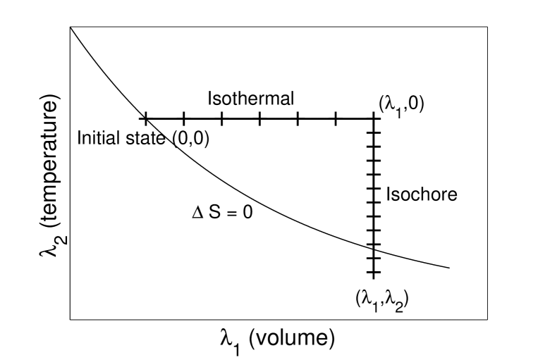
To determine the isentrope curve, we compute the entropy variation along a given path in $(\lambda_{1},\lambda_{2})$ space going through the reference initial state, and search for the point such that the entropy difference with this state is 0. A simple choice is illustrated in Fig. 2. It consists in performing

1. an isothermal rarefaction, going from the initial compressed state $(0,0)$ to an intermediate state $(\lambda_{1},0)$ with $\lambda_{1}\geq 0$;

2. in a second step, an isochore cooling, going from the intermediate state $(\lambda_{1},0)$ to some final state $(\lambda_{1},\lambda_{2})$, resorting to a maximal temperature difference $\lambda_{2}\Delta T<0$ large enough.

The idea is that, in general, the first part of the transformation increases the entropy of the system (since more space becomes available for the particles), while the entropy decreases in the second part (since the temperature decreases). Of course, more general paths, with joint variations of $\lambda_{1}$ and $\lambda_{2}$, could be considered.

The energies $\langle H\rangle_{V(\lambda_{1}),T(\lambda_{2})}$ are computed using standard sampling strategies, while the remainder in the expression of ${\mathcal{S}}(\lambda_{1},\lambda_{2})-{\mathcal{S}}(0,0)$, a ratio of partition functions, is estimated using standard techniques for free-energy calculations. This is detailed in Appendix A.

We emphasize that this procedure is time consuming since it requires many equilibrium samplings to obtain one point on the curve. It is however exact (up to statistical errors and discretization errors in the integrals defining $A$), and can be straightforwardly parallelized since the equilibrium samplings required are independent.

III.2 Successive hugoniostat simulations

The variations of macroscopic quantities across a shock interface are governed by the Rankine-Hugoniot relations, which relate the jumps of the quantities under investigation (pressure, density, velocities) to the velocity of the shock front. The third Rankine-Hugoniot conservation law for the Euler equation governing the hydrodynamic evolution of the fluid reads (macroscopic quantities are denoted by curly letters)

$$\mathcal{H}=\mathcal{U}-\mathcal{U}_{0}-\frac{1}{2}(\mathcal{P}+\mathcal{P}_{0})(V_{0}-V)=0.$$ (7)

In this expression, $\mathcal{U}$ is the internal energy of the fluid, $\mathcal{P}$ its pressure, and $V$ its volume. The subscript $0$ refers to the initial state (the pole), the other quantities are evaluated at a state obtained from some shock compression, after equilibration. The Hugoniot curve corresponds to all the possible states satisfying (7). In practice, the collection of these states may be computed by nonequilibrium simulations with shocks of different strengths, inducing various compressions.

Alternatively, small equilibrium simulations may be used, relying on the statistical physics reformulation of the Hugoniot relation:

$${\mathcal{H}}(\lambda_{1},\lambda_{2})-{\mathcal{H}}(0,0) = \langle H\rangle_{V(\lambda_{1}),T(\lambda_{2})}-\langle H\rangle_{V(0),T(0)}$$ (8)

$$+\frac{\lambda_{1}}{2}V(0)\left(\langle P_{xx}\rangle_{V(\lambda_{1}),T(\lambda_{2})}+\langle P_{xx}\rangle_{V(0),T(0)}\right)=0.$$

The $xx$ component of the pressure tensor is, for a simulation domain of volume $V(\lambda_{1})$,

$$P_{xx}(q,p)=\frac{1}{V(\lambda_{1})}\sum_{i=1}^{N}\frac{p_{i,x}^{2}}{m_{i}}-q_{i,x}\,\partial_{q_{i,x}}U(q).$$ (9)

For a given variation of the volume for instance (indexed by $\lambda_{1}$), the variation $\lambda_{2}T\delta T$ of the temperature is sought for, using for instance the techniques described in Refs. Maillet et al., 2000; Maillet and Stoltz, 2009.

The Hugoniot curve does not have a priori any relationship with the isentrope curve. However, it can be shown that the entropy variation along the Hugoniot curve is negligible up to terms of order three in the volume variable; the Hugoniot and the isentropic curves are osculatory. We present in Appendix B two proofs, the standard proof based on thermodynamic relations, and a new proof fully relying on a statistical physics reformulation.

The good agreement between the Hugoniot and the isentrope for small compressions and/or expansions can be used to compute the isentropic curve as a succession of weak shocks or weak releases, this approximation getting more accurate as the shock compressions are weakened. The only parameter left in this method is the relative volume change $\delta V/V=\lambda_{1}^{n+1}-\lambda_{1}^{n}$ during the instantaneous compressions or releases. We used the Hugoniostat methodMaillet et al. (2000); Maillet and Stoltz (2009) to compute a sequence of states $(\lambda_{1}^{n},\lambda_{2}^{n})$ such that $\mathcal{H}(\lambda_{1}^{n+1},\lambda_{2}^{n+1})=\mathcal{H}(\lambda_{1}^{n},\lambda_{2}^{n})$, the corresponding thermodynamic properties at these states being obtained as a by-product of the simulation.

III.3 Isentropic integration

Another way to perform thermodynamic integration along an isentropic path has been proposed by Desjarlais.Desjarlais The method relies on the equilibrium evaluation of $\displaystyle\frac{\partial{\mathcal{P}}}{\partial{\mathcal{U}}}$ (see Eq. (11) below). It could be applied to a system where the pressure is not isotropic upon replacing the pressure observable by the $xx$ component of the pressure tensor.

The total differential of the entropy can be written as:

$$d{\mathcal{S}}=\frac{\partial{\mathcal{S}}}{\partial T}\bigg{|}_{V}dT+\frac{\partial{\mathcal{S}}}{\partial V}\bigg{|}_{T}dV.$$ (10)

For constant entropy processes,

$$\frac{\partial{\mathcal{S}}}{\partial T}\bigg{|}_{V}=\frac{1}{T}\frac{\partial{\mathcal{U}}}{\partial T}\bigg{|}_{V}=-\frac{\partial{\mathcal{P}}}{\partial T}\bigg{|}_{V},\qquad\frac{\partial{\mathcal{S}}}{\partial V}\bigg{|}_{T}=\frac{\partial{\mathcal{P}}}{\partial T}\bigg{|}_{V},$$

so that, along the isentrope,

$$\frac{dT}{T}=-\frac{\displaystyle\frac{\partial{\mathcal{P}}}{\partial T}\bigg{|}_{V}}{\displaystyle\frac{\partial{\mathcal{U}}}{\partial T}\bigg{|}_{V}}\,dV=-\frac{\partial{\mathcal{P}}}{\partial{\mathcal{U}}}\bigg{|}_{V}dV.$$

This equation can be integrated as

$$\frac{T_{2}}{T_{1}}=\exp\left(-\int_{V_{1}}^{V_{2}}{\frac{\partial{\mathcal{P}}}{\partial{\mathcal{U}}}\bigg{|}_{V}dV}\right),$$ (11)

giving the temperature $T_{2}$ at which the system at volume $V_{2}$ has the same entropy as the system in the reference state $(T_{1},{\mathcal{P}}_{1})$. This formula is evaluated in practice by discretizing the integral appearing in the exponential, and approximating the integrand using standard canonical sampling procedues. We refer to Appendix C for more precisions.

III.4 Evaluation of the entropy based on the chemical potential

This technique, which can be used only for systems in a fluid phase, follows the classical methodology of computing the free energy $\mathcal{F}$ of a system starting from the thermodynamic relation:Kofke and Cummings (1997)

$$\mathcal{F}={\mathcal{U}}-T{\mathcal{S}}=N\mu-{\mathcal{P}}V,$$ (12)

where $\mu$ is the chemical potential, defined in the canonical ensemble as

$$\mu=\frac{\partial\mathcal{F}}{\partial N}.$$ (13)

In the case of a canonical simulation, all thermodynamic quantities are functions of the volume and the temperature, so that

$${\mathcal{S}}=\frac{{\mathcal{U}}(T,V)+N\mu(T,V)-{\mathcal{P}}(T,V)V}{T}.$$ (14)

This expression allows to compute the absolute entropy of the system provided the chemical potential is known,Smith et al. (2006) the average pressure and energy being computed using standard sampling techniques. The chemical potential is estimated using the Widom insertion method.

IV Numerical results for release waves

We compare in this section the results for the different techniques presented in Sections II and III, for a release in a Lennard-Jones system (argon). The aim is to assess whether the release is indeed isentropic, and also to demonstrate that approximate equilibrium computations for small systems (successive Hugoniostat, isentropic integration) can approximate the isentrope curve obtained from the more rigourous and costly thermodynamic integration technique.

IV.1 Numerical parameters

IV.1.1 Initial state.

We consider argon in an initial shocked state, located on the Hugoniot curve for a compression such that $L_{x}=cL$ with $c=0.65$, and corresponding to $T=1758$ K and $P=1.7\times 10^{10}$ Pa. At these thermodynamic conditions, the system is in a liquid state. The interactions within noble gas atoms are well-described by a Lennard-Jones potential:

$$V(q_{1},\dots,q_{N})=\sum_{1\leq i<j\leq N}v(|q_{i}-q_{j}|),\qquad v(r)=4\varepsilon\left(\left(\frac{\sigma}{r}\right)^{12}-\left(\frac{\sigma}{r}\right)^{6}\right).$$

In the case of Argon, $\varepsilon/k_{\rm B}=120$ K and $\sigma=3.405$ Å. The cut-off radius for the Lennard-Jones interaction is here $r_{\rm cut}=2.5\sigma$.

IV.1.2 Nonequilibrium simulations.

In order to reach this initial state before performing the NEMD release, a preliminary hugoniostat simulation is run for a system of $50\times 50\times 500$ unit cells, using periodic boundary conditions. Then, the boundary conditions in the longitudinal direction are removed, and the system evolves according to the Hamiltonian dynamics. Profiles of thermodynamic quantities are computed every 0.25 ps for the post-processing procedure described at the end of Section II.2.

IV.1.3 Equilibrium simulations

Equilibrium computations have been performed with a system composed of $N=4000$ atoms, starting in a FCC crystal geometry before melting, using periodic boundary conditions in all directions.

Thermodynamic integration.

As shown in Section III.1, the search of states having the same entropy can be performed using thermodynamic integration, which amounts to performing many equilibrium simulations. The canonical sampling for a given set of parameters $(\lambda_{1},\lambda_{2})$ is done with a Langevin dynamics for $N_{\rm steps}=2^{17}$ time steps, with $\Delta t=2\times 10^{-15}$ s, and a friction coefficient $\gamma=10^{13}$ s^-1.

First, the entropy variation along the isothermal release is computed, with canonical samplings along the path $(0,0)\to(0,\lambda_{1})$ with $\lambda_{1}=0.54$ (using $M+1=15$ states). Then, for each compression of interest, the isochore cooling is performed using temperature steps $\Delta T=-25$ K for expansions $\lambda_{1}\leq 0.25$, and $\Delta T=-50$ K for states $\lambda_{1}\geq 0.25$ (these paths can be restated in terms of $\lambda_{2}\in[0,1]$ upon considering a temperature modification $\Delta T$ depending on the compression). The numerical integration for computing the value of $A$ is finally performed using the trapezoidal rule.

Error estimates on the canonical samplings are obtained with block averaging.Flyvberg and Petersen (1989) In all the cases considered, the statistical error (as measured using the 95% confidence interval associated with the variance computed from block-averaging) is inferior to 1%. Therefore, the entropy difference is computed within 1% errors. For fixed $\lambda_{1}$, the state $\lambda_{2}$ such that ${\mathcal{S}}(\lambda_{1},\lambda_{2})$ is constant is then known with an error depending on the local value of the partial derivative of ${\mathcal{S}}$ with respect to $\lambda_{2}$. This error can immediately be reformulated as an error on the estimated temperature. The error on the computed pressure is the error arising from the error on the state $\lambda_{2}$, plus the sampling error. It is found to be at most 2%.

Successive Hugoniostat.

Successive Hugoniostat simulations have been performed with a Langevin version of the Hugoniostat method (see Eq. (11) in Ref. Maillet and Stoltz, 2008, with the parameters $\xi=10^{12}$ s^-1 and $\nu=10^{12}$ s^-1). Trajectories of $N_{\rm steps}=50,000$ timesteps at each compression are considered, with a timestep $\Delta t=5\times 10^{-16}$ s. The relative volume change $\delta V/V_{0}$ from one point on the curve to another is set to 0.01.

Isentropic integration.

See Appendix C.

Entropy evaluation.

The test particle insertion method used to evaluate the chemical potential requires many more iterations than the other equilibrium techniques. In the same framework as for isentropic integration (see Appendix C), $N_{\rm steps}=5\times 10^{8}$ iterations were needed to obtain a satisfactory convergence. The statistical error on the calculated entropy (as measured using the 95% confidence interval associated with the variance computed from block-averaging) is estimated to be inferior to 1.2 %.

IV.2 Discussion of the numerical results

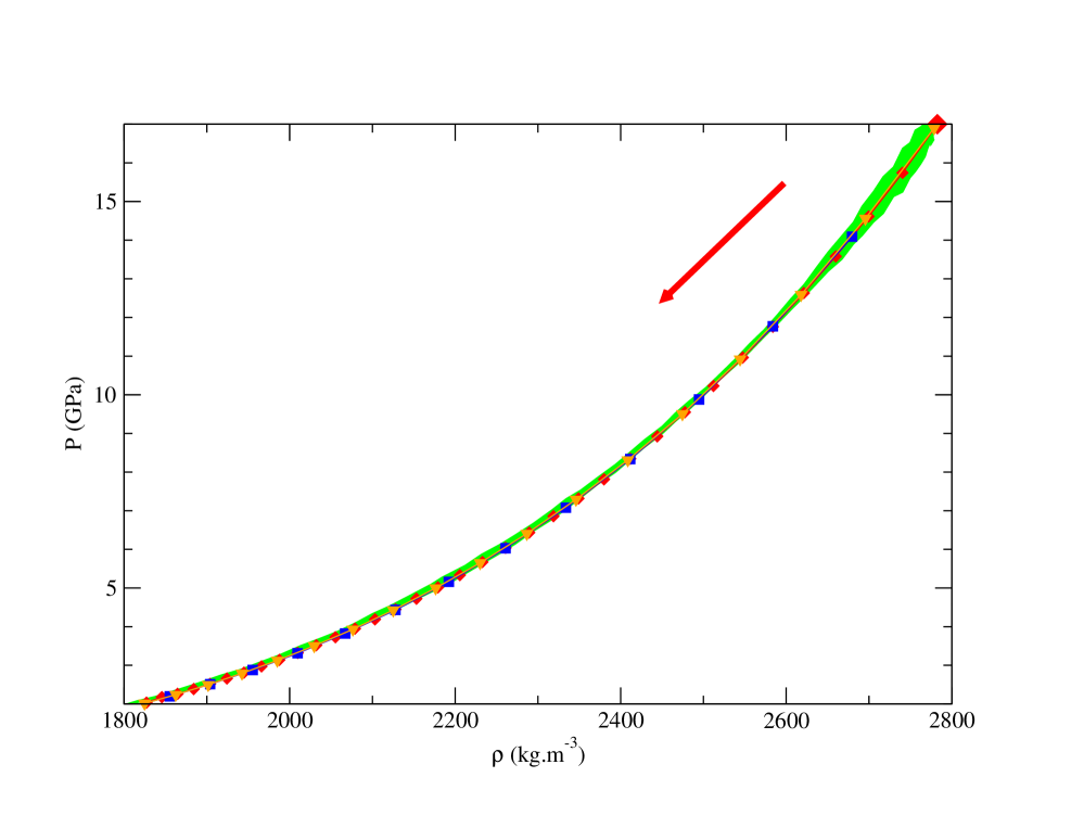
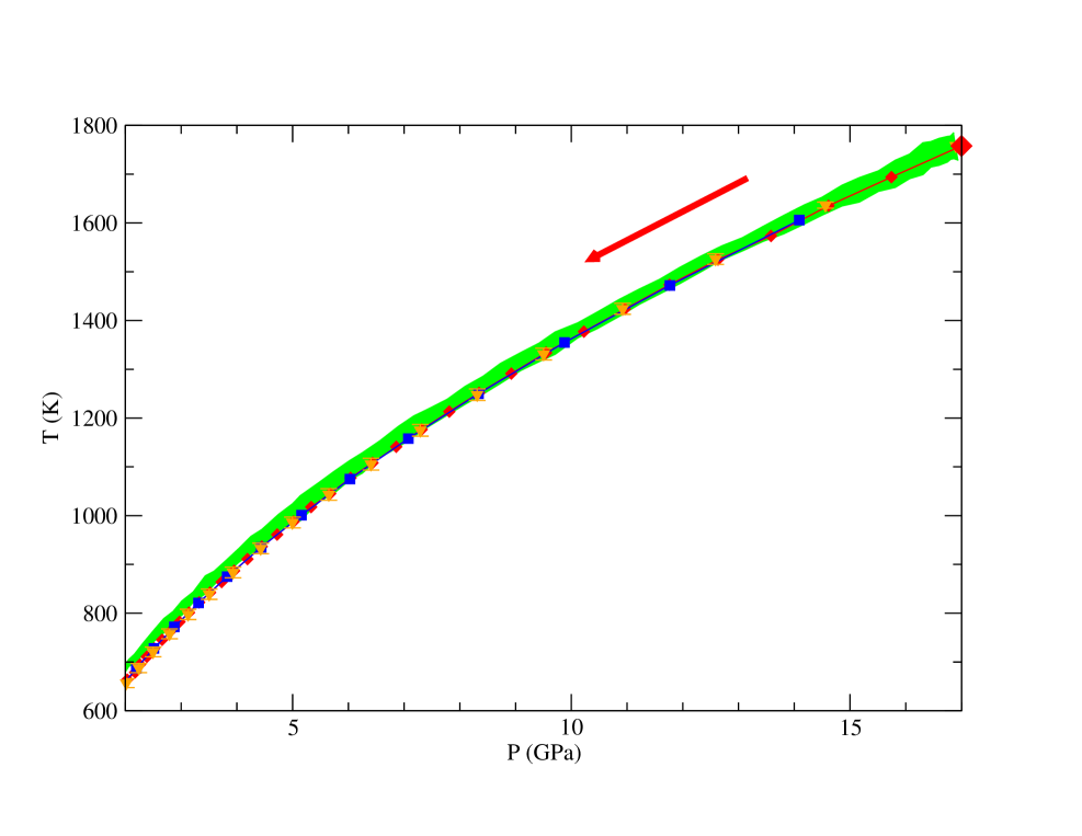
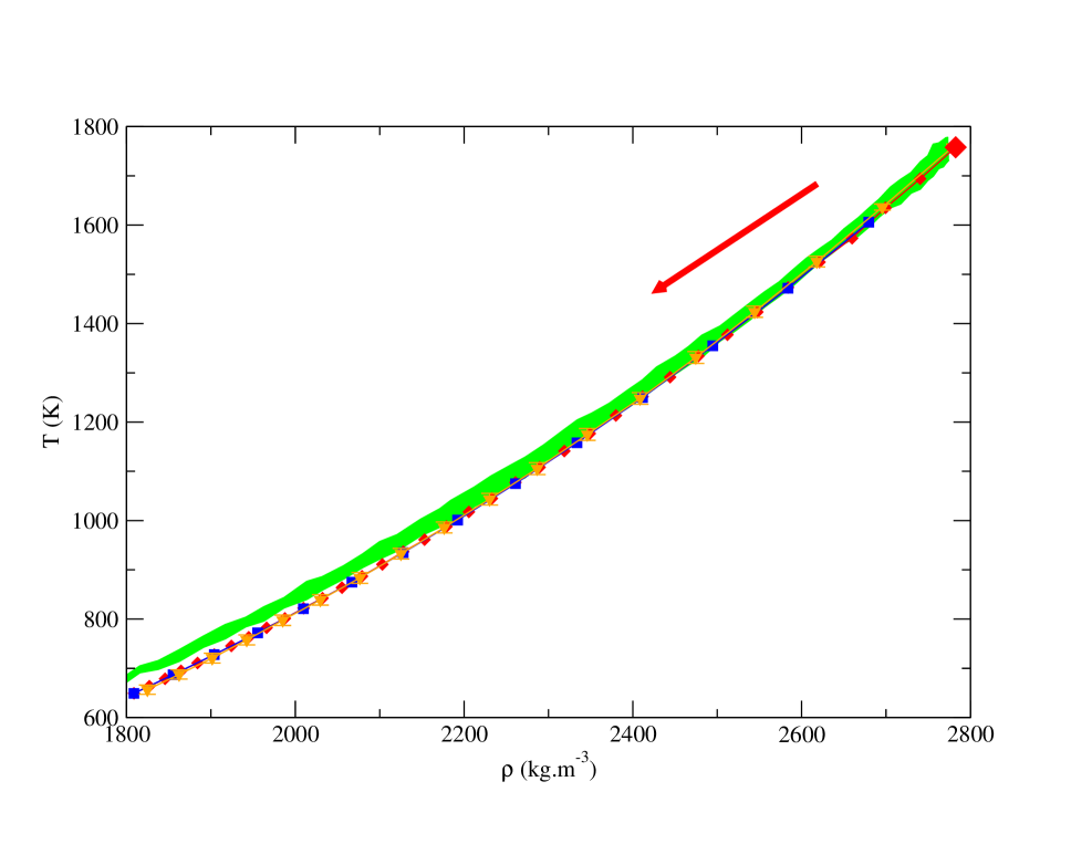
Release waves are presented in Figures 3-5 in three different diagrams, $(P,\rho)$,$(P,T)$ and $(T,\rho)$. It can clearly be seen that the results coming from the three equilibrium techniques of isentropic simulations are very close. This shows that provided the relative volume change parameter is carefully chosen in either the successive hugoniostat method or the isentropic integration, the propagating error remains at a low level; these methods can then be as accurate as the more rigorous and costly method of thermodynamic integration. Moreover, evaluating the chemical potential, we have computed absolute value of the entropy at three densities, $\rho=2780$ kg.m^-3, $\rho=2190$ kg.m^-3, and $\rho=1806$ kg.m^-3. The corresponding values, $83.2\pm 0.95$ J.mol^-1, $83.1\pm 0.42$ J.mol^-1, $83.2\pm 0.18$ J.mol^-1, confirm that the entropy is indeed constant (within the error bars) on the calculated curve, validating once again the different methods.

The comparison with the results of the expansion of the liquid using nonequilibrium MD is also fruitful. The overall agreement is fair enough, which means that release waves are indeed almost isentropic. However, it can be noticed that the temperature is not predicted correctly. While the different curves look very similar in a ($P,\rho$) diagrams, some discrepancies appear in the ($T,P$) diagram, which are even more obvious in the ($T,\rho$) diagram. Indeed, for the latter diagram, the observed temperatures around the final density are greater than the error bars. The thermodynamic path followed by the system during its release exhibits systematically a higher temperature than the one of an isentropic process. This means that the release of a monoatomic liquid is not strictly isentropic, as is sometimes expected or assumed.

Recall however that a release is expected to be isentropic only for non-turbulent flows of non-viscous fluids. In the case considered here, the fluid has a finite, non zero viscosity, and therefore dissipates energy under the form of heat. As a consequence, the temperature should be higher than for an isentropic release. A tentative of evaluation of this effect is presented below. On the Hugoniot curve, viscous effects can be introduced in the Hugoniot relationFickett and Davis (1979) by means of the ”viscous pressure” $\pi$ as

$$\frac{1}{2}\pi(\mathcal{V}_{0}-\mathcal{V})=\mathcal{U}-\mathcal{U}_{0}-\frac{1}{2}(\mathcal{P}+\mathcal{P}_{0})(V_{0}-V),$$ (15)

where $\pi$ is defined as

$$\pi=-\nu\frac{du}{dx},$$ (16)

$\nu$ being the fluid viscosity and $\displaystyle\frac{du}{dx}$ the velocity gradient. Taking the viscosity of the argon fluid at $T=700$ K and $P=1$ GPa (the most extremes conditions of available thermodynamic tables), and considering an average velocity gradient (taken during the fluid release), we find a temperature elevation of a few Kelvins. Considering that the pressure is much higher in our simulation, and therefore that the viscosity should be also greater, the actual temperature increase due to the finite viscosity should rather be of the order of a few tens of Kelvins, which is consistent with what can be observed in our numerical results.

Finally, a purely nonequilibrium effect has been observed during the NEMD simulations, that also leads to a temperature increase in the system. Indeed, gradients of thermodynamic and kinematic quantities are large at the first stages of the release, when the hot and dense material is in contact with void. The thermodynamic path followed by the system at those early stages of the simulation does not correspond to the thermodynamic path followed when the release has reached its self-similarity regime. Some equilibration time is needed for some steady-state regime to be reached. We evaluated this time to be around 5 picoseconds.

V Conclusion

We have presented or recalled several equilibrium methods to compute isentropic processes in the high pressure regime, either for compressions or releases. These methods, although very different in nature, lead to similar results when applied to the release of a monoatomic liquid.

We have then compared release waves computed with these equilibrium methods with the nonequilibrium simulation of the release process. The results show that the release is almost, but not strictly isentropic, the system’s temperature being systematically greater than the one of the isentropic process. This is the consequence of two effects. First, the fluid actually has a finite viscosity and therefore dissipates heat, leading to a temperature increase. To our knowledge, this is the first time that this effect has been quantified rigorously using molecular dynamics simulations. Moreover, the thermodynamic path followed by the system during its release takes some time to reach a converged profile. We anticipate that these effects will be enhanced in the case of a more complex fluid, for example in the case of a the release of detonation product. Therefore, the assumption that release waves are isentropic should be carefully verified in each case.

Appendix A Practical implementation of the thermodynamic integration

A.1 Reformulation of the problem in a fixed geometry

From a computational viewpoint, it is more convenient to work with a fixed simulation domain. For instance, the unperturbed domain $V(0)$ may be used to fix the geometry of the system. The volume variations are then rephrased as variations in the interaction scale between the particles in the direction of compression or release. In the same vein, the temperature may be kept constant, upon rescaling the interactions strengh by a factor depending on the temperature variation. Introducing the rescaled potential energy for a configuration $q=(x,y,z)$:

$$U_{\lambda_{1},\lambda_{2}}(q)=\frac{1}{1+\lambda_{2}\delta T}U((1+\lambda_{1})x,y,z).$$

and the associated Hamiltonian

$$H_{\lambda_{1},\lambda_{2}}(q,p)=U_{\lambda_{1}}(q)+\frac{1}{1+\lambda_{2}\delta T}\sum_{i=1}^{N}\frac{p_{i}^{2}}{2m_{i}},$$

canonical averages for a volume $V(\lambda_{1})$ at a temperature $T(\lambda_{2})$ can be reformulated as canonical averages in terms of the rescaled Hamiltonian $H_{\lambda_{1},\lambda_{2}}$ at the reference state at volume $V(0)$ and temperature $T(0)$. More precisely,

$$\langle H\rangle_{V(\lambda_{1}),T(\lambda_{2})}=\frac{3N}{2}k_{\rm B}T(\lambda_{2})+(1+\lambda_{2}\delta T)\langle\langle U_{\lambda_{1},\lambda_{2}}\rangle\rangle_{\lambda_{1},\lambda_{2}},$$

where

$$\langle\langle f\rangle\rangle_{\lambda_{1},\lambda_{2}}=\frac{\displaystyle\int_{\Omega(0)}f(q,p)\,{\mathrm{e}}^{-H_{\lambda_{1},\lambda_{2}}(q,p)/k_{\rm B}T(0)}\,dq\,dp}{\displaystyle\int_{\Omega(0)}{\mathrm{e}}^{-H_{\lambda_{1},\lambda_{2}}(q,p)/k_{\rm B}T(0)}\,dq\,dp}.$$

It is then easily seen that

$${\mathcal{S}}(\lambda_{1},\lambda_{2})-{\mathcal{S}}(0,0) = \frac{3N}{2}\ln(1+\lambda_{2}\delta T)+N\ln(1+\lambda_{1})$$

$$+\beta\left[\langle\langle U_{\lambda_{1},\lambda_{2}}\rangle\rangle_{\lambda_{1},\lambda_{2}}-\langle\langle U_{0,0}\rangle\rangle_{0,0}\right]$$

$$+A(\lambda_{1},\lambda_{2}),$$

with

$$A(\lambda_{1},\lambda_{2})=\ln\left(\frac{\displaystyle\int_{V(0)^{N}}{\mathrm{e}}^{-\beta U_{\lambda_{1},\lambda_{2}}(q)}\,dq}{\displaystyle\int_{V(0)^{N}}{\mathrm{e}}^{-\beta U_{0,0}(q)}\,dq}\right).$$

In the above expression of the entropy difference, the first line is the ideal gas contribution to the entropy difference. As a consistency check, we can verify that the entropy increases when the volume or the temperature is increased, as expected. The terms on the second and third lines in Eq. (A.1) are the “excess” contributions associated with the potential interaction energy.

A.2 Numerical evaluation of the different terms

To estimate ${\mathcal{S}}$, two quantities are required:

1. averages $\langle\langle\cdot\rangle\rangle_{\lambda_{1},\lambda_{2}}$ with respect to the Hamiltonian $H_{\lambda_{1},\lambda_{2}}$ are computed using standard sampling techniques such as a Langevin dynamics at an inverse temperature $\beta$, implemented using the so-called BBK algorithm.Brünger et al. (1984) Of course, many other sampling techniques could be used to estimate this canonical average, in particular Nosé-Hoover dynamicsNosé (1984); Hoover (1985) or Metropolis-Hastings schemesMetropolis et al. (1953); Hastings (1970) (see Ref. Cancès et al., 2007 for a mathematical review on sampling methods in the context of molecular simulation);

2. the term $A(\lambda_{1},\lambda_{2})$ requires more care in its estimation. Since this term is a ratio of partition functions, standard techniques used for the computation of free energy differences may be used. We resorted to thermodynamic integration,Kirkwood (1935) in which case the function is rewritten as the integral of some canonical averages:

   $$A(\lambda_{1},\lambda_{2})=\int_{0}^{\lambda_{1}}\frac{\partial A}{\partial_{\lambda_{1}}}(x,0)\,dx+\int_{0}^{\lambda_{2}}\frac{\partial A}{\partial_{\lambda_{2}}}(\lambda_{1},x)\,dx,$$

   with

   $$\frac{\partial A}{\partial\lambda_{2}}(\lambda_{1},\lambda_{2})=\beta\,\frac{\delta T}{1+\lambda_{2}\delta T}\,\langle\langle U_{\lambda_{1},\lambda_{2}}\rangle\rangle_{\lambda_{1},\lambda_{2}},$$ (18)

   and

   $$\frac{\partial A}{\partial\lambda_{1}}(\lambda_{1},\lambda_{2})=\big{\langle}\big{\langle}\,x\cdot\nabla_{x}U((1+\lambda_{1})x,y,z)\,\big{\rangle}\big{\rangle}_{\lambda_{1},\lambda_{2}}.$$ (19)

In conclusion, the numerical procedure consists in first estimating the derivatives of the function $A$ and the average potential energy, for as many points as required on the thermodynamic path chosen. Approximations of ${\mathcal{S}}$ can then be obtained thanks to (A.1), after a numerical integration to obtain $A$. The entropy difference along the path is then plotted, and fixing the volume change $\lambda_{1}$, the temperature variation is chosen such that the entropy difference is 0. This determines $\lambda_{2}$ as a function of $\lambda_{1}$.

Appendix B Relationship between the Hugoniot and the isentrope curves at the pole

We present in this Appendix two proofs of the fact that the isentrope curve and the Hugoniot agree at order 3 in the volume change. The first one is a standard thermodynamic proof, but the second one, based on statistical physics relations, is new to the best of our knowledge.

B.1 Standard thermodynamic proof

For the sake of completeness, we reproduce here the proof of Ref. Thouvenin, 1997. From the thermodynamic relation $Td{\mathcal{S}}=d{\mathcal{U}}+{\mathcal{P}}\,dV$ and from the Hugoniot relation ${\mathcal{U}}={\mathcal{U}}_{0}+\frac{1}{2}({\mathcal{P}}+{\mathcal{P}}_{0})(V_{0}-V)$, the entropy variation along the Hugoniot curve can be computed. One derivation leads to

$$T\left(\frac{d{\mathcal{S}}}{dV}\right)_{\rm Hug}={\mathcal{P}}+\left(\frac{d{\mathcal{U}}}{dV}\right)_{\rm Hug}=\frac{1}{2}({\mathcal{P}}-{\mathcal{P}}_{0})+\frac{1}{2}(V_{0}-V)\left(\frac{d{\mathcal{P}}}{dV}\right)_{\rm Hug}.$$ (20)

A second derivation gives

$$T\frac{d^{2}{\mathcal{S}}_{\rm Hug}}{dV^{2}}+\frac{d{\mathcal{S}}_{\rm Hug}}{dV}\frac{dT_{\rm Hug}}{dV}=\frac{1}{2}(V_{0}-V)\frac{d^{2}{\mathcal{P}}_{\rm Hug}}{dV^{2}}.$$ (21)

With a final derivation,

$$T\frac{d^{3}{\mathcal{S}}_{\rm Hug}}{dV^{3}}+2\frac{d^{2}{\mathcal{S}}_{\rm Hug}}{dV^{2}}\frac{dT_{\rm Hug}}{dV}+\frac{d{\mathcal{S}}_{\rm Hug}}{dV}\frac{d^{2}T_{\rm Hug}}{dV^{2}}=-\frac{1}{2}\frac{d^{2}{\mathcal{P}}_{\rm Hug}}{dV^{2}}+\frac{1}{2}(V_{0}-V)\frac{d^{3}{\mathcal{P}}_{\rm Hug}}{dV^{3}}.$$ (22)

At the initial state (denoted with a subscript 0), that is, in the limit $V\to V_{0}$, it holds:

$$\left(\frac{d{\mathcal{S}}_{\rm Hug}}{dV}\right)_{0} = 0,$$

$$\left(\frac{d^{2}{\mathcal{S}}_{\rm Hug}}{dV^{2}}\right)_{0} = 0,$$

$$T_{0}\left(\frac{d^{3}{\mathcal{S}}_{\rm Hug}}{dV^{3}}\right)_{0} = -\frac{1}{2}\left(\frac{d^{2}{\mathcal{P}}}{dV^{2}}\right)_{0}\not=0.$$

The entropy variation along the Hugoniot curve is therefore of order three in volume, and the Hugoniot and the isentropic curves are osculatory.

B.2 A statistical physics derivation

Without loss of generality (and for notational simplicity), we may set ${\mathcal{H}}(0,0)={\mathcal{S}}(0,0)=0$ since we are only interested in differences of $\mathcal{F}$ and $\mathcal{S}$.

B.2.1 Some useful relations.

The derivatives of the function $A$ are useful for comparing the Hugoniot and the isentrope relations. The average $xx$ component of the pressure tensor for the volume $V(\lambda_{1})$ and the temperature $T(\lambda_{2})$ is obtained by averaging the observable

$$P_{xx}(q,p)=\frac{1}{V(\lambda_{1})}\left(Nk_{\rm B}T(\lambda_{2})-x\cdot\nabla_{x}U(q)\right).$$

Therefore,

$$\langle P_{xx}\rangle_{V(\lambda_{1}),T(\lambda_{2})} = \frac{N}{(1+\lambda_{1})V(0)}\,k_{\rm B}T(\lambda_{2})-\frac{1}{V(\lambda_{1})}\frac{\displaystyle\int_{V(\lambda_{1})^{N}}x\cdot\nabla_{x}U(q)\,{\mathrm{e}}^{-U(q)/k_{\rm B}T(\lambda_{2})}\,dq}{\displaystyle\int_{V(\lambda_{1})^{N}}{\mathrm{e}}^{-U(q)/k_{\rm B}T(\lambda_{2})}\,dq}$$

$$= \frac{N}{\beta V(0)}\,\frac{1+\lambda_{2}\delta T}{1+\lambda_{1}}-\frac{1+\lambda_{1}}{V(\lambda_{1})}\frac{\displaystyle\int_{V(0)^{N}}x\cdot\nabla_{x}U((1+\lambda_{1})x,y,z)\,{\mathrm{e}}^{-\beta U_{\lambda_{1},\lambda_{2}}(q)}\,dq}{\displaystyle\int_{V(0)^{N}}{\mathrm{e}}^{-\beta U_{\lambda_{1},\lambda_{2}}}}.$$

This shows that, using (19),

$$\langle P_{xx}\rangle_{V(\lambda_{1}),T(\lambda_{2})}=\frac{N}{\beta V(0)}\,\frac{1+\lambda_{2}\delta T}{1+\lambda_{1}}+\frac{1+\lambda_{2}\delta T}{\beta V(0)}\frac{\partial A}{\partial_{\lambda_{1}}}(\lambda_{1},\lambda_{2}).$$

B.2.2 Hugoniot curve.

With the above computations, it is easily seen that the Hugoniot relation (8) can be restated as

$$\beta{\mathcal{H}}(\lambda_{1},\lambda_{2}) = \frac{3N}{2}\lambda_{2}\delta T+\beta\left[(1+\lambda_{2}\delta T)\langle\langle U_{\lambda_{1},\lambda_{2}}\rangle\rangle_{\lambda_{1},\lambda_{2}}-\langle\langle U_{0,0}\rangle\rangle_{0,0}\right]$$

$$+\frac{N\lambda_{1}}{2}\left(\frac{1+\lambda_{2}\delta T}{1+\lambda_{1}}+1\right)+\frac{\lambda_{1}}{2}\left(\frac{\partial A}{\partial_{\lambda_{1}}}(0,0)+(1+\lambda_{2}\delta T)\frac{\partial A}{\partial_{\lambda_{1}}}(\lambda_{1},\lambda_{2})\right).$$

B.2.3 Comparison between the Hugoniot and the isentrope.

We now Taylor expand the difference $\beta{\mathcal{H}}(\lambda_{1},\lambda_{2})-{\mathcal{S}}(\lambda_{1},\lambda_{2})$ up to the third order, i.e. neglecting a remainder term $r(\lambda_{1},\lambda_{2})$ which is such that $|r(\lambda_{1},\lambda_{2})|\leq C(|\lambda_{1}|+\lambda_{2}|)^{3}$. We denote such remainders by ${\mathrm{O}}(\lambda^{3})$ in the sequel. It holds

$$\beta{\mathcal{H}}(\lambda_{1},\lambda_{2})-{\mathcal{S}}(\lambda_{1},\lambda_{2}) = \frac{3N}{2}(\lambda_{2}\delta T-\ln(1+\lambda_{2}\delta T))+N\left(\frac{\lambda_{1}}{2}\left(1+\frac{1}{1+\lambda_{1}}\right)-\ln(1+\lambda_{1})\right)$$

$$+\lambda_{1}\lambda_{2}\frac{\delta T}{2}\left(\frac{N}{1+\lambda_{1}}+\frac{\partial A}{\partial_{\lambda_{1}}}(\lambda_{1},\lambda_{2})\right)+\beta\lambda_{2}\delta T\langle\langle U_{\lambda_{1},\lambda_{2}}\rangle\rangle_{\lambda_{1},\lambda_{2}}$$

$$+\frac{\lambda_{1}}{2}\left(\frac{\partial A}{\partial_{\lambda_{1}}}(0,0)+\frac{\partial A}{\partial_{\lambda_{1}}}(\lambda_{1},\lambda_{2})\right)-A(\lambda_{1},\lambda_{2}).$$

Introducing the notation

$$A_{i}=\frac{\partial A}{\partial_{\lambda_{i}}}(0,0),\qquad A_{ij}=\frac{\partial^{2}A}{\partial_{\lambda_{i}}\partial_{\lambda_{j}}}(0,0),$$

the Taylor expansions of the function $A$ and its first derivatives at an arbitrary state $(\lambda_{1},\lambda_{2})$ read (using $A(0,0)=0$):

$$A(\lambda_{1},\lambda_{2})=\lambda_{1}A_{1}+\lambda_{2}A_{2}+\frac{\lambda_{1}^{2}}{2}A_{11}+\lambda_{1}\lambda_{2}A_{12}+\frac{\lambda_{2}^{2}}{2}A_{22}+{\mathrm{O}}(\lambda^{3}),$$

$$\frac{\partial A}{\partial_{\lambda_{i}}}(\lambda_{1},\lambda_{2})=A_{i}+\lambda_{1}A_{i1}+\lambda_{2}A_{i2}+{\mathrm{O}}(\lambda^{2}).$$

With these Taylor expansions and the relation (18), it is straightforward to show that

$$\beta{\mathcal{H}}(\lambda_{1},\lambda_{2})-{\mathcal{S}}(\lambda_{1},\lambda_{2}) = \frac{3N}{4}\lambda^{2}_{2}\delta T^{2}+\lambda_{1}\lambda_{2}\frac{\delta T}{2}\left(N+A_{1}\right)+\lambda_{2}(1+\lambda_{2}\delta T)\frac{\partial A}{\partial_{\lambda_{2}}}(\lambda_{1},\lambda_{2})$$

$$= \frac{\lambda_{2}\delta T}{2}\left[\lambda_{1}\left(N+A_{1}+\frac{A_{12}}{\delta T}\right)+\lambda_{2}\left(\frac{3N}{2}\delta T+2A_{2}+\frac{A_{22}}{\delta T}\right)\right]+{\mathrm{O}}(\lambda^{3}).$$

Using (18), the derivatives of the entropy differences can be computed:

$$\frac{\partial{\mathcal{S}}}{\partial\lambda_{1}}(\lambda_{1},\lambda_{2})=\frac{N}{1+\lambda_{1}}+\frac{\partial A}{\partial\lambda_{1}}(\lambda_{1},\lambda_{2})+\frac{1+\lambda_{2}\delta T}{\delta T}\frac{\partial^{2}A}{\partial\lambda_{1}\partial\lambda_{2}}(\lambda_{1},\lambda_{2}),$$

$$\frac{\partial{\mathcal{S}}}{\partial\lambda_{2}}(\lambda_{1},\lambda_{2})=\frac{3N\delta T}{2(1+\lambda_{2}\delta T)}+2\frac{\partial A}{\partial\lambda_{2}}(\lambda_{1},\lambda_{2})+\frac{1+\lambda_{2}\delta T}{\delta T}\frac{\partial^{2}A}{\partial^{2}\lambda_{2}}(\lambda_{1},\lambda_{2}).$$

This shows that

$$\beta{\mathcal{H}}(\lambda_{1},\lambda_{2})-{\mathcal{S}}(\lambda_{1},\lambda_{2})=\frac{\lambda_{2}\delta T}{2}\left(\lambda_{1}\frac{\partial{\mathcal{S}}}{\partial\lambda_{1}}(0,0)+\lambda_{2}\frac{\partial{\mathcal{S}}}{\partial\lambda_{2}}(0,0)\right)+{\mathrm{O}}(\lambda^{3}),$$ (23)

so that, since

$${\mathcal{S}}(\lambda_{1},\lambda_{2})={\mathcal{S}}(0,0)+\lambda_{1}\frac{\partial{\mathcal{S}}}{\partial\lambda_{1}}(0,0)+\lambda_{2}\frac{\partial{\mathcal{S}}}{\partial\lambda_{2}}(0,0)+{\mathrm{O}}(\lambda^{2}),$$

and ${\mathcal{S}}(0,0)=0$, it holds

$$\beta{\mathcal{H}}(\lambda_{1},\lambda_{2})-\left(1+\frac{\lambda_{2}\delta T}{2}\right){\mathcal{S}}(\lambda_{1},\lambda_{2})={\mathrm{O}}(\lambda^{3}).$$ (24)

This relation shows immediately that ${\mathcal{H}}(\lambda_{1},\lambda_{2})={\mathrm{O}}(\lambda^{3})$ on the isentrope, and so, the initial slopes of the curves, and their first derivatives, coincide.

Appendix C Precisions on the isentropic integration

Several numerical schemes may be used to integrate (11). The simplest one consists in approximating the integral appearing in the exponential factor with a Riemman formula using the value of the integrated function on the left side of the interval:

$$T_{2}\simeq T_{1}\exp\left(-\frac{\partial{\mathcal{P}}}{\partial{\mathcal{U}}}\bigg{|}_{V_{1}}(V_{2}-V_{1})\right).$$ (25)

Of course, higher order integration methods could be used.

It remains to decide how to compute the derivative $\displaystyle\frac{\partial{\mathcal{P}}}{\partial{\mathcal{U}}}\bigg{|}_{V_{1}}$. Finite differences may be used to this end, but this would require at least two very carefully converged simulations with volumes $V_{1}\pm\Delta V$. It seems more appealing to compute the partial derivative using standard fluctuations formulas:Lagache et al. (2001); Bourasseau et al. (2007)

$$\frac{\partial{\mathcal{U}}}{\partial T}\bigg{|}_{V_{1}}=C_{v}(V_{1},T_{1})=\frac{3}{2}Nk_{\rm B}+\frac{1}{k_{\rm B}T_{1}2}\left(\left\langle U^{2}\right\rangle_{V_{1},T_{1}}-\left\langle U\right\rangle^{2}_{V_{1},T_{1}}\right),$$ (26)

and

$$\frac{\partial{\mathcal{P}}}{\partial T}\bigg{|}_{V_{1}}=\frac{Nk_{\rm B}}{V_{1}}+\frac{1}{k_{\rm B}T_{1}^{2}}\left(\left\langle PH\right\rangle_{V_{1},T_{1}}-\left\langle P\right\rangle_{V_{1},T_{1}}\left\langle H\right\rangle_{V_{1},T_{1}}\right),$$ (27)

where $C_{v}(V_{1},T_{1})$ is the specific heat at constant volume, and the pressure observable for a simulation domain of volume $V_{1}$ reads

$$P(q,p)=\frac{1}{3V_{1}}\sum_{i=1}^{N}\frac{p_{i}^{2}}{m_{i}}-q_{i}\cdot\nabla_{q_{i}}U(q).$$ (28)

The partial derivative $\partial{\mathcal{P}}/\partial{\mathcal{U}}$ can then be evaluated in a single simulation at $(N,V_{1},T_{1})$ using (26)-(27).

The numerical implementation of this method is done as follows. The partial derivative of the pressure with respect to the energy is first computed with a Monte Carlo simulation for the given initial conditions $(N,V_{1},T_{1})$. The temperature $T_{2}$ is then evaluated from Eq. (25). The partial derivative is next computed at volume $V_{2}$ to predict the next temperature. Proceeding incrementally, the whole isentrope curve can be constructed.

The numerical results presented in this work have been obtained by performing canonical samplings with a Metropolis algorithm, using the Monte-Carlo Gibbs code. Partial derivatives have been computed in the NVT ensemble. The convergence of simple thermodynamic averages was generally obtained after $N_{\rm steps}=10^{7}$ iterations, but derivative properties (related to the covariance of some observables) required about $N_{\rm steps}=10^{8}$ iterations for a satisfactory convergence. Error estimates on the canonical samplings have been obtained with block averaging,Flyvberg and Petersen (1989) and the error propagation estimated along the integration scheme has been computed using standard propagation rules. In all the cases considered, the statistical error (as measured using the 95% confidence interval associated with the variance computed from block-averaging) on the predicted temperature on the isentrope curve is inferior to 1.5 %.

Caption list:

Figure 1: (a) (color online) Non-Equilibrium Molecular Dynamics of isentropic release waves. The four pictures represent snapshots of the system during the release process, the expansion proceeding in the longitudinal $x$ direction. Atoms are colored according to their potential energies (scaling corresponding to $-1.38\times 10^{-20}$ J for blue up to $7.55\times 10^{-20}$ J for red).

Figure 1: (b) (color online) Density profiles taken at different times of the simulation (from blue to red as time increases).

Figure 2: Path in the $(\lambda_{1},\lambda_{2})$ space used to compute states with the same entropy as the initial state. Each cross represents some equilibrium canonical sampling along the thermodynamic path. First, the isothermal expansion is performed (horizontal line in the diagram), starting from the initial state $(0,0)$, until the required density is reached. The entropy of the state $(\lambda_{1},0)$ is $S_{\rm init}+\Delta S_{\rm expansion}$. Then, an isochore cooling is performed ($\lambda_{1}$ is kept fixed; vertical line in the diagram), until the entropy difference during this process is the opposite of the entropy variation found in the expansion part. The final state $(\lambda_{1},\lambda_{2})$, located at the intersection of the curve $\Delta S=0$ and the vertical line, has then the same entropy as the initial state.

Figure 3: (color online) Isentropic release in a ($P,\rho$) diagram. Symbols represent results from equilibrium methods, red diamonds for the successive hugoniostat, blue squares for the thermodynamic integration and yellow triangles for the entropy integration. NEMD results are plotted in green, the width of the so-obtained tube corresponding to the error bars. The arrow indicates the path followed during the release.

Figure 4: (color online) Isentropic release in a ($T,P$) diagram. The symbols are the same as in Figure 3. Notice that there is slight deviation of the NEMD results for the lowest temperatures.

Figure 5: (color online) Isentropic release in a ($T,\rho$) diagram. The symbols are the same as in Figure 3. There is a noticeable deviation of the NEMD results for the lowest temperatures.

Figure 1:

(a)

Fig 1: (b)

Figure 2:

Figure 3:

Figure 4:

Figure 5:

References

- Tasker et al. (2003) D. Tasker, J.H.Goforth, H. Oona, J. King, D. Herrera, and D. Torres (2003), In proceedings of the AIP conference Shock Compression and Condensed Matter, Portland, Oregon.
- Tasker et al. (2005) D. Tasker, J. Goforth, H. Oona, P. Rigg, D. Koller, J. King, D. Herrera, D. Torres, F. Sena, F. Abeyta, et al. (2005), In proceedings of the AIP conference Shock Compression and Condensed Matter, Baltimore, Maryland.
- Lyzenga and Ahrens (1981) G. Lyzenga and T. Ahrens (1981), In proceedings of the AIP conference Shock Compression and Condensed Matter, Menlo Park, California.
- Barker (1983) L. Barker (1983), In proceedings of the AIP conference Shock Compression and Condensed Matter, Santa Fe, New Mexico.
- Perez (1988) M. Perez, J. Phys. Colloque C3 49, 713 (1988).
- Nguyen et al. (2006) J. Nguyen, D. Orlikowski, F. Streitz, N. Holmes, and J. Moriarty, J. Appl. Phys. 100, 023508 (2006).
- Barnes et al. (1974) J. Barnes, P. Blewett, R. McQueen, K. Meyer, and D. Venable, J. Appl. Phys. 45, 727 (1974).
- Tsypkin et al. (1975) V. Tsypkin, V. Mineev, A. Ivanov, V. Svidinskii, and B. Rozhdestvenskii, Sov. Phys. Tech. Phys. 20, 387 (1975).
- Frenkel and Smit (2002) D. Frenkel and B. Smit, Understanding Molecular Simulation - From Algorithms to Applications (Academic Press, 2002).
- Allen and Tildesley (1987) M. Allen and D. Tildesley, Computer Simulation of Liquids (Oxford University Press, Oxford, 1987).
- Holian and Lomdahl (1998) B. Holian and P. Lomdahl, Science 280, 2085 (1998).
- Maillet et al. (2000) J.-B. Maillet, M. Mareschal, L. Soulard, R. Ravelo, P. S. Lomdahl, T. C. Germann, and B. L. Holian, Phys. Rev. E 63, 016121 (2000).
- Maillet and Stoltz (2009) J.-B. Maillet and G. Stoltz, Applied Mathematics Research Express 2008, abn004 (2009).
- Bourasseau et al. (2007) E. Bourasseau, V. Dubois, N. Desbiens, and J.-B. Maillet, J. Chem. Phys. 127, 084513 (2007).
- Bernard and Maillet (2002) S. Bernard and J.-B. Maillet, Phys. Rev. B. 66, 012103 (2002).
- Balian (2007) R. Balian, From Microphysics to Macrophysics. Methods and Applications of Statistical Physics, vol. I - II (Springer, 2007).
- Verlet (1967) L. Verlet, Phys. Rev. 159, 98 (1967).
- (18) M. Desjarlais, Workshop on accelerator-driven warm dense matter, 2006.
- Kofke and Cummings (1997) D. Kofke and P. Cummings, Mol. Phys. 92, 973 (1997).
- Smith et al. (2006) W. Smith, M. Lísal, and I. Nezbeda, Chem. Phys. Lett. 426, 436 (2006).
- Flyvberg and Petersen (1989) H. Flyvberg and H. G. Petersen, J. Chem. Phys. 91, 461 (1989).
- Maillet and Stoltz (2008) J.-B. Maillet and G. Stoltz, arXiv preprint 0807.0558 (2008).
- Fickett and Davis (1979) W. Fickett and W. Davis, Detonation (dover publication, 1979).
- Brünger et al. (1984) A. Brünger, C. L. Brooks, and M. Karplus, Chem. Phys. Lett. 105, 495 (1984).
- Nosé (1984) S. Nosé, J. Chem. Phys. 81, 511 (1984).
- Hoover (1985) W. G. Hoover, Phys. Rev. A 31, 1695 (1985).
- Metropolis et al. (1953) N. Metropolis, A. W. Rosenbluth, M. N. Rosenbluth, A. H. Teller, and E. Teller, J. Chem. Phys. 21, 1087 (1953).
- Hastings (1970) W. K. Hastings, Biometrika 57, 97 (1970).
- Cancès et al. (2007) E. Cancès, F. Legoll, and G. Stoltz, Math. Model. Numer. Anal. 41, 351 (2007).
- Kirkwood (1935) J. G. Kirkwood, J. Chem. Phys. 3, 300 (1935).
- Thouvenin (1997) J. Thouvenin, Détonique (CEA, 1997).
- Lagache et al. (2001) M. Lagache, P. Ungerer, A. Boutin, and A. Fuchs, Phys. Chem. Chem. Phys. 3, 4333 (2001).