Statefinder diagnostic in a torsion cosmology
Abstract
We apply the statefinder diagnostic to the torsion cosmology, in which an accounting for the accelerated universe is considered in term of a Riemann-Cartan geometry: dynamic scalar torsion. We find that there are some typical characteristic of the evolution of statefinder parameters for the torsion cosmology that can be distinguished from the other cosmological models. Furthermore, we also show that statefinder diagnostic has a direct bearing on the critical points. The statefinder diagnostic divides the torsion parameter into differential ranges, which is in keeping with the requirement of dynamical analysis. In addition, we fit the scalar torsion model to ESSENCE supernovae data and give the best fit values of the model parameters.
pacs:
98.80.-k, 98.80.Es1 Introduction
The current observations, such as SNeIa (Supernovae type Ia), CMB (Cosmic Microwave Background) and large scale structure, converge on the fact that a spatially homogeneous and gravitationally repulsive energy component, referred as dark energy, accounts for about % of the energy density of universe. Some heuristic models that roughly describe the observable consequences of dark energy were proposed in recent years, a number of them stemming from a certain physics [1] and the others being purely phenomenological [2]. Dark energy can even behave as a phantom and effectively violate the weak energy condition[3].
In various cosmological models, fundamental quantities are either geometrical (if they are constructed from a spacetime geometry directly) or physical (if they depend upon physical fields). Physical quantities are certainly model-dependent, while geometrical quantites are more universal. About thirty years ago, the bouncing cosmological model with torsion was suggested in Ref.[4], but the torsion was imagined as playing role only at high densities in the early universe. Goenner et al. made a general survey of the torsion cosmology [5], in which the equations for all the PGT (Poincaré Gauge Theory of gravity) cases were discussed although they only solved in detail a few particular cases. Recently some authors have begun to study torsion as a possible reason of the accelerating universe [6]. Nester and collaborators [7] consider an accounting for the accelerated universe in term of a Riemann-Cartan geometry: dynamic scalar torsion. They explore the possibility that the dynamic PGT connection, reflecting the nature of dynamic PGT torsion, provides the accelerating force. With the usual assumptions of homogeneity and isotropy in cosmology and specific cases of the suitable parameters and initial conditions, they find that torsion field could play a role of dark energy.
One of the motivation was to avoid singularities in the initial investigations of torsion cosmology [8]. However, it soon was found that non-linear torsion effects were more likely to produce stronger singularities [9]. The non-linear effects turn out to play a key role for the outstanding present day mystery: the accelerated universe. In the various PGT, the connection dynamics decomposed into six modes with certain spin and parity: , , . Some investigations showed that may well be the only acceptable dynamic PGT torsion modes [10]. The pseudoscalar mode is naturally driven by the intrinsic spin of elementary fermions, therefore it naturally interacts with such sources. Consequently, it is generally thought that axial torsion must be small and have small effects at the late time of cosmological evolution. This is a major reason why one does not focus on this mode at the late time. On the other hand, the scalar mode does not interact in any direct obvious fashion with any known type of matter [11], therefore one can imagine it as having significant magnitude and yet not being conspicuously noticed. Furthermore, there is a critical non-zero value for the affine scalar curvature since mode can interact indirectly through the non-linear equations. The homogeneity and isotropy of cosmology have received strong confirmation from modern observations, which greatly restrict the possible types of non-vanishing fields. Under the assumption of homogeneity and isotropy, mode has only a time component and it can be specified as the gradient of a time-dependent function. Therefore, the cosmological models with the scalar mode offer a situation where dynamic torsion may lead to observable effect at late time. We emphasize again that one does not focus on the early universe, where one could indeed expect large effects (though their signature would have to be separated from other large effects), and substitutionally asks about traces of torsion effects at the late time of cosmological evolution [7].
Obviously, the fine-tuning problem is one of the most important issues for the torsion cosmology [7]. And a good model should limit the fine-tuning as much as possible. The dynamical attractor of the cosmological system has been employed to make the later time behaviors of the model insensitive to the initial condition of the field and thus alleviates the fine-tuning problem [12]. Furthermore, Nester et al [7] have shown that the Hubble parameter and have an oscillatory form for the scalar torsion cosmology.
The traditional geometrical parameters, i.e., the Hubble parameter and the deceleration parameter , are two elegant choices to describe the expansion state of universe but they can not distinguish various accelerating mechanism uniquely, because a quite number of models may just correspond to the same current values of and . However, Sahni, Saini, Starobinsky and Alam [13] have introduced the statefinder pair : , . It is obviously a natural next step beyond and . Fortunately, as is shown in the literatures [14, 15], the statefinder parameters which are also geometrical diagnostics, are able to differentiate a series of cosmological models successfully. Using the discussion of statefinder parameters in the scalar torsion cosmology, we explain easily why the present field equations modify the expansion of the universe only at late time. If the evolving trajectory of statefinder have a decelerating phase () at early time, then we can understand why the expansion of the universe until remains unchanged in the scalar torsion models.
In this paper, we apply the statefinder diagnostics to the torsion cosmology. We find that there are some characteristics of statefinder parameters for the torsion cosmology that can be distinguished from the other cosmological models. The statefinder diagnostics show that the universe naturally has an accelerating expansion at low redshifts (late time) and a decelerating expansion at high redshifts (early time). Therefore, scalar torsion cosmology can avoid some of the problems which occur in other models. Especially, the effect of torsion can make the expansion rate oscillate when torsion parameter or . Whether the universe has properties which are easier to explain within the scalar torsion context is a remarkable possibility demanding further exploration. The oscillatory feature of Hubble parameter had earlier been reported for the braneworld cosmology [16] and the quasi-steady state cosmology [17]. We show that statefinder diagnostic has a direct bearing on the critical points of the dynamical system. One of the most interesting characteristic of the trajectories is that there are loop and curves with the shape of tadpole in the case of the torsion parameter . In this case, we fit the scalar torsion model to current type Ia supernova data and find it is consistent with the observations. Furthermore, we analyze preliminarily the relevance for realistic observation of the found statefinder parameters.
2 The equations of motion
PGT [18] has been regarded as an interesting alternative to general relativity because of its gauge structure and geometric properties. PGT based on a Riemann-Cartan geometry, allows for dynamic torsion in addition to curvature. The affine connection of the Riemann-Cartan geometry is
| (2.1) |
where is the Levi-Civita connection and is the torsion tensor. Meantime, the Ricci curvature and scalar curvature can be written as
| (2.2) | |||||
| (2.3) |
where and are the Riemannian Ricci curvature and scalar curvature, respectively, and is the covariant derivative with the Levi-Civita connection (For a detailed discussion see Ref. [7].). Theoretical analysis of PGT led us to consider tendentiously dynamic ”scalar mode”. In this case, the restricted expression of the torsion can be written as [7]
| (2.4) |
where the vector is the trace of the torsion. Then, the Ricci curvature and scalar curvature can be expressed as
| (2.5) | |||||
| (2.6) |
The gravitational Lagrangian density for the scalar mode is
| (2.7) |
where and is a torsion parameter. Consider that the parameter is associated with quadratic scalar curvature term , so that should be positive [7]. Therefore, the field equations of the scalar mode are
| (2.8) | |||
| (2.9) |
where is the source energy-momentum tensor and is the contribution of the scalar torsion mode to the effective total energy-momentum tensor:
| (2.10) | |||||
Since current observations favor a flat universe, we will work in the spatially flat Robertson-Walker metric , where is the scalar factor. This engenders the Riemannian Ricci curvature and scalar curvature:
| (2.11) | |||
| (2.12) | |||
| (2.13) |
where is the scalar factor, and is the Hubble parameter. The torsion should also be only time dependent, therefore one can let ( is the torsion field) and the spatial parts vanish. The corresponding equations of motion in the matter-dominated era are as follows
| (2.14) | |||||
| (2.15) | |||||
| (2.16) |
where and the energy density of matter component
| (2.17) |
One can scale the variables and the parameters as
| (2.18) |
where is the present value of Hubble parameter and is the Planck length. Under the transform (2.18), Eqs. (2.14)-(2.16) remain unchanged. After transform, new variables , , and , and new parameters , , and are all dimensionless. Obviously, the Newtonian limit requires .
For the case of scalar torsion mode, the effective energy-momentum tensor can be represented as
| (2.19) | |||||
| (2.20) |
and the off-diagonal terms vanish. The effective energy density
| (2.21) |
which is deduced from general relativity. is an effective pressure, and the effective equation of state is
| (2.22) |
which is induced by the dynamic torsion.
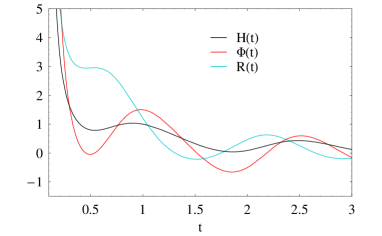
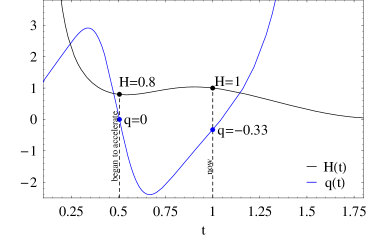
In the case of , Nester et al showed that the scalar mode can contribute an oscillating aspect to the expansion rate of the universe [7]. This oscillatory nature can be illustrated in Fig. 1 where we have chosen , , , , and set the current time . According to scaling (2.18), the present value of the Hubble parameter is unity. Obviously, is damped-oscillating at late time and is negative today, which means the expansion of the universe is currently accelerating. The value of turns from positive to negative when the time is around , which is the epoch the universe began to accelerate.
However, the above result is dependent on the choice of initial data and the values of the parameters. Then, the scalar torsion cosmology is unsuited to solving the fine-tuning problem in the case of . In the following sections, we’ll investigate the statefinder and give the dynamics analysis for all ranges of the parameter .
3 Statefinder diagnostic
For the spatially flat CDM model the statefinder parameters correspond to a fixed point while for the standard cold dark matter model (SCDM) containing no radiation. Since the torsion cosmology have used the dynamic scalar torsion (a geometry quantity in the Riemann-Cartan spacetime), the torsion accelerating mechanism is bound to exhibit an essential distinction in contrast with various dark energy models. Therefore, its statefinder diagnostic is sure to reveal differential feature. Let us now study the torsion cosmological model in detail. Using Eqs. (2.14)-(2.17), we have the deceleration parameter
| (3.1) |
and the statefinder parameters
| (3.2) |
and
| (3.3) |
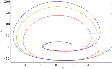
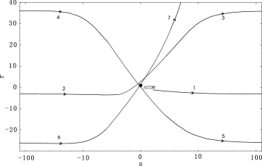
In the following we will discuss the statefinder for four differential ranges of the torsion parameter , respectively. Firstly, we consider the time evolution of the statefinder pairs and in the case of . In Fig. 2, we plot evolution trajectories in the and planes, where we have chosen and . We see easily that cosmic expansion alternates between deceleration and acceleration in the evolving trajectories of plane, and the amplitude becomes larger and larger as increase of time. The trajectories in the plane is quite complicated, so we mark its sequence by the ordinal number. Every odd number curve evolves from finite to infinite, but even number curve evolves from infinite to finite. These are quasi-periodic behaviors which corresponds to the numerical solution of Ref. [7]. Noticeably, the trajectories will never pass CDM point .
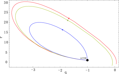
Secondly, we discuss the time evolution of the statefinder pairs and for the case of . We plot evolving trajectories in Fig. 3, where we have chosen and . We see clearly that the cosmic acceleration is guaranteed by the dynamic scalar torsion in the evolving trajectories of plane, and the curves will converge into CDM point. The evolving trajectories go through a climbing-up stage first, then get into a rolling-down stage in the plane. Lastly, trajectories tend to CDM point . Furthermore, the only one forms a loop that starts from then evolves back to , and others show in the shape of tadpole.

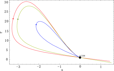
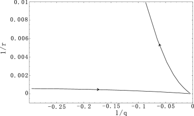
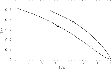
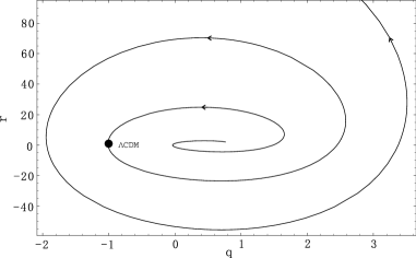
Thirdly, we discuss the time evolution of the trajectories for the case of . We plot evolving trajectories in Fig. 4, where we have chosen and . Obviously, the cosmic acceleration can happen since deceleration parameter is negative. , and become larger and larger first, then less and less as the cosmic time increase.
Finally, we consider the time evolution of the statefinder pairs and in the case of . In Fig. 5, we plot evolving trajectories in the and planes, where we have chosen and . We find easily that the evolving trajectories analogous to the case of except trajectories pass the CDM point.
To sum up, it is very interesting to see that the scalar torsion naturally provide the accelerating force in the universe for any torsion parameter . However, it is dependent on torsion parameters that there is a decelerating () expansion before an accelerating () expansion. The statefinder diagnostics show that the universe naturally has an accelerating expansion at low redshifts (late time) and a decelerating expansion at high redshifts (early time) for the cases of and . Obviously, scalar torsion cosmology can avoid some of the problems which occur in other models. If we refuse the possibility of non-positivity of the kinetic energy, we will employ normal assumption, i. e., . In this case, the effect of torsion can make the expansion rate oscillate. With suitable adjustments of the torsion parameters, it is possible to change the quasi-period of the expansion rate as well as its amplitudes. It is worth noting that the true values of the statefinder parameters of the universe should be determined in model-independent way. In principle, can be extracted from some future astronomical observations, especially the SNAP-type experiment.
Why there are new features for the statefinder diagnostic of torsion cosmology? Why the torsion parameter is divided into differential ranges by the statefinder diagnostic? Answer is very simple. In fact, the statefinder diagnostic has a direct bearing on the attractor of cosmological dynamics. Therefore, we will discuss the dynamic analysis in next section.
4 Dynamics analysis
Eqs. (2.14)-(2.16) is an autonomous system, so we can use the qualitative method of ordinary differential equations. Critical points are always exact constant solutions in the context of autonomous dynamical systems. These points are often the extreme points of the orbits and therefore describe the asymptotic behavior. If the solutions interpolate between critical points they can be divided into a heteroclinic orbit and a homoclinic orbit (a closed loop). The heteroclinic orbit connects two different critical points and homoclinic orbit is an orbit connecting a critical point to itself. In the dynamical analysis of cosmology, the heteroclinic orbit is more interesting [19]. If the numerical calculation is associated with the critical points, then we will find all kinds of heteroclinic orbits.
According to equations (2.14)-(2.16), we can obtain the critical points and study the stability of these points. Substituting linear perturbations , and near the critical points into three independent equations, to the first orders in the perturbations, gives the evolution of the linear perturbations, from which we could yield three eigenvalues. Stability requires the real part of all eigenvalues to be negative. There are five critical points of the system as follows
where , and . The corresponding eigenvalues of the critical points (i)-(v) are
| (4.2) |
Using Eq. (LABEL:criticalpoints), we find that there is only a critical point in the case of . From Eq. (4.2), the corresponding eigenvalue is , so is an asymptotically stable focus. If we consider the linearized equations, then Eqs. (2.14)-(2.16) are reduced to
| (4.3) |
The linearized system (4.3) has an exact periodic solution
| (4.4) |
where , , and , and are initial values. Obviously, is a critical line of center for the linearized Eqs. (4.4). In other words, there are only exact periodic solutions for the linearized system, but there are quasi-periodic solutions near the focus for the coupled nonlinear equations. This property of quasi-periodic also appears in the statefinder diagnostic with the case of .
| critical points | property | stability | |
|---|---|---|---|
| (i) | saddle | unstable | |
| (ii) | positive attractor | -1 | stable |
| (iii) | negative attractor | -1 | unstable |
| (iv) | saddle | -1 | unstable |
| (v) | saddle | -1 | unstable |
| critical points | property | stability | |
|---|---|---|---|
| (i) | focus | stable | |
| (ii) | saddle | -1 | unstable |
| (iii) | saddle | -1 | unstable |
| (iv) | saddle | -1 | unstable |
| (v) | saddle | -1 | unstable |
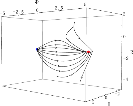
In the case of , the critical point (ii) is a late time de Sitter attractor and (iii) is a negative attractor. The properties of the critical points are shown in table 1. The de Sitter attractor indicates that torsion cosmology is an elegant scheme and the scalar torsion mode is an interesting geometric quantity for physics. In the dynamical analysis of cosmology, the heteroclinic orbit is more interesting. Using numerical calculation, we plot the heteroclinic orbit connects the critical point case (iii) to case (ii) in Fig. 6. This heteroclinic orbit is just corresponding to the loop in Fig. 3, which is from CDM point to CDM point. Furthermore, the trajectories with the shape of tadpole correspond to saddles.
In the case of , there is only an unstable saddle where the effective equation of state tends to . Therefore, the trajectories in Fig. 4 show that , and become larger and larger, then less and less as time increases.
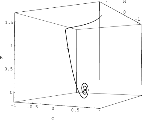
In the case of , the properties of the critical points are shown in table 2. The trajectories correspond to the stable focus (see Fig. 6) and unstable saddles with . Therefore, the trajectories pass through the CDM point.
5 Fit the torsion parameters to supernovae date
In Ref.[7], the authors have compared the numerical values of the torsion model with the observational data, in which they fixed the initial values , and , and torsion parameters and . In this section, we fixed the initial value, then fit the torsion parameters to current type Ia supernovae data.
The scalar torsion cosmology predict a specific form of the Hubble parameter as a function of redshifts in terms of two parameters and when we chose initial values. Using the relation between and the comoving distance (where is the redshift of light emission)
| (5.1) |
and the light ray geodesic equation in a flat universe where is the scale factor.
In general, the approach towards determining the expansion history is to assume an arbitrary ansatz for which is not necessarily physically motivated but is specially designed to give a good fit to the data for . Given a particular cosmological model for where are model parameters, the maximum likelihood technique can be used to determine the best fit values of parameters as well as the goodness of the fit of the model to the data. The technique can be summarized as follows: The observational data consist of apparent magnitudes and redshifts with their corresponding errors and . These errors are assumed to be gaussian and uncorrelated. Each apparent magnitude is related to the corresponding luminosity distance by
| (5.2) |
where is the absolute magnitude. For the distant SNeIa, one can directly observe their apparent magnitude and redshift , because the absolute magnitude of them is assumed to be constant, i.e., the supernovae are standard candles. Obviously, the luminosity distance is the ‘meeting point’ between the observed apparent magnitude and the theoretical prediction . Usually, one define distance modulus and express it in terms of the dimensionless ‘Hubble-constant free’ luminosity distance defined by as
| (5.3) |
where the zero offset depends on (or ) as
| (5.4) |
The theoretically predicted value in the context of a given model can be described by [20]
| (5.5) |
Therefore, the best fit values for the torsion parameters () of the model are found by minimizing the quantity
| (5.6) |
Since the nuisance parameter is model-independent, its value from a specific good fit can be used as consistency test of the data [21] and one can choose a priori value of it (equivalently, the value of dimensionless Hubble parameter ) or marginalize over it thus obtaining
| (5.7) |
where
| (5.8) |
| (5.9) |
and
| (5.10) |
In the latter approach, instead of minimizing , one can minimize which is independent of .
The Eqs. (2.8-2.10) can be solved explicitly by a series in the form
| (5.11) |
where and
| (5.12) | |||
Using the general relation between Hubble parameter and the redshift , can be written as a function of
| (5.13) |
However, the convergence radius of the series (5.11) is , so we can use the expansion directly in the case of the redshift being . By the numerical calculation, we find that corresponds to for the valuses of parameters and in the Fig. 9. For the case of , we should use a direct analytic continuation. Weierstrass [22] had built the whole theory of analytic functions from the concept of power series. Given a point (), the function has a Taylor expansion
| (5.14) |
where the coefficients is still expressed as Eq. (5) and can be decided by Eq. (5.11). The new series defines an analytic function which is said to be obtained from by direct analytic continuation. This process can be repeated any number of times. In the general case we have to consider a succession of power series , ,…,, each of which is a direct analytic continuation of the preceding one. By using this method we have the evolution of Hubble parameter . Furthermore, we have the function from Eq. (5.13). In fact, we need only to consider the case of for the ESSENCE supernovae data.
We now apply the above described maximum likelihood method using the ESSENCE supernovae data which is one of the reliable published data set consisting of 192 SNeIa (). Beside the 162 data points given in table 9 of Ref. [23], which contains 60 ESSENCE SNeIa, 57 SNLS SNeIa and 45 nearby SNeIa, we add 30 SNeIa detected at by the Hubble Space Telescope [24] as in Ref.[25].
In table 3, we show the best fit of torsion parameters at different initial values of and .
| 0.25 | 0.35 | -0.10 | 1.44 |
| 0.20 | 0.34 | -0.08 | 1.80 |
| 0.15 | 0.34 | -0.06 | 2.40 |
| 0.10 | 0.33 | -0.04 | 3.60 |
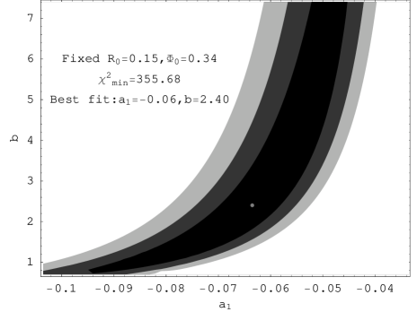
In Fig. 9, contours with 68.3%, 95.4% and 99.7% confidence level are plotted, in which we take a marginalization over the model-independent parameter . The best fit as showed in the figure corresponds to and , and the minimum value of . For , one can get and the best fit . Therefore, it’s easy to know that is consistent at the level with the best fits of scalar torsion cosmology. In Fig. 8, we show a comparison of the ESSENCE supernovae data along with the theoretically predicted curves in the context of scalar torsion and . We can see that the scalar torsion model(, , , ) gives a close curve behavior to the one from (). Clearly, the allowed ranges of the parameters and favor the case of if we chose and .


6 Conclusion and discussion
We have studied the statefinder diagnostic to the torsion cosmology, in which an accounting for the accelerated universe is considered in term of a Riemann-Cartan geometry: dynamic scalar torsion. We have shown that statefinder diagnostic has a direct bearing on the critical points. The statefinder diagnostic divides the torsion parameter into four ranges, which is in keeping with the requirement of dynamical analysis. Therefore, the statefinder diagnostic can be used to an exceedingly general category of models including several for which the notion of equation of state is not directly applicable. The statefinder diagnostic has the advantage over the dynamical analysis at the simplicity, but the latter can provide more information.
The most interesting characteristic of the trajectories is that there is a loop in the case of . This behavior corresponds to the heteroclinic orbit connecting the negative attractor and de Sitter attractor. The trajectories with the shape of tadpole show that they pass through the CDM fixed point along the time evolution, then the statefinder pairs are going along with a loop and they will pass through the CDM fixed point again in the future. It is worth noting that there exists closed loop in the Ref. [14], but there is no closed loop which contains the CDM fixed point. These behaviors indicate that torsion cosmology is an elegant scheme and the scalar torsion mode is an interesting geometric quantity for physics. Furthermore, the quasi-periodic feature of trajectories in the cases of or shows that the numerical solutions in Ref. [7] are not periodic, but are quasi-periodic near the focus for the coupled nonlinear equations.
We fixed only the initial values, then fitted the torsion parameters to current SNeIa dataset. We find that the scalar torsion naturally explain the accelerating expansion of the universe for any torsion parameter . However, it is dependent and that there is a decelerating expansion before an accelerating expansion. The statefinder diagnostics show that the universe naturally have an accelerating expansion at late time and a decelerating expansion at early time for the case of and . If we refuse the possibility of non-positivity of the kinetic energy, we have to employ normal assumption (). Under this assumption, the effect of torsion can make the expansion rate oscillate. Furthermore, with suitable adjustments of the torsion parameters and initial value, it is possible to change the quasi-period of expansion rate as well as its amplitudes. In order to have a quantitative understanding of the scalar torsion cosmology, the matter density , the effective mass density , and the quantity are important. This scenario bears a strong resemblance to the braneworld cosmology in a very different context by Sahni, Shtanov and Viznyuk [26]. The parameters in the torsion cosmology and in the CDM cosmology can nevertheless be quite different. Therefore, at high redshift, the torsion cosmology asymptotically expands like a matter-dominated universe with the value of inferred from the observations of the local matter density. At low redshift, the torsion model behaves like CDM but with a renormalized value of . The difference between and is dependent on the present value of statefinder parameters . A more detailed estimate, however, lies beyond the scope of the present paper, and we will study it in a future work. Finally, and should be extracted from some future astronomical observations in principle, especially the SNAP-type experiments.
Acknowledgments
This work is supported by National Science Foundation of China grant No. 10847153 and No. 10671128.
References
References
-
[1]
Sahni V and Starobinsky A 2000 Int. J. Mod. Phys.
D9 373 [astro-ph/9904398]
Peebles P J E and Ratra B 2003 Rev. Mod. Phys. 75 559 [astro-ph/0207347]
Padmanabhan T 2003 Phys. Rept. 380 235 [hep-th/0212290]
Copeland E J, Sami M and Tsujikawa S 2006 Int. J. Mod. Phys. D15 1753 [hep-th/0603057]
Sahni V and Starobinsky A 2006 Int. J. Mod. Phys. D15 2105 [astro-ph/0610026] -
[2]
Endo M and Fukui T 1977 Gen. Rel. Grav. 8
833
Overduin J M and Cooperstock F I 1998 Phys. Rev. D58 043506 [astro-ph/9805260]
Hao J G and Li X Z 2005 Phys. Lett. B606 7 [astro-ph/0404154]
Liu D J and Li X Z 2005 Phys. Lett. B611 8 [astro-ph/0501596]
Beesham A 1993 Phys. Rev D48 3539 -
[3]
Caldwell R R 2002 Phys. Lett. B545 23 [astro-ph/9908168]
Sahni V and Shtanov Yu 2003 JCAP 11 014 [astro-ph/0202346]
Hao J G and Li X Z 2003 Phys. Rev. D67 107303 [gr-qc/0302100]
Liu D J and Li X Z 2003 Phys. Rev. D68 067301 [hep-th/0307239]
Li X Z and Hao J G 2004 Phys. Rev. D69 107303 [hep-th/0303093]
Hao J G and Li X Z 2003 Phys. Rev. D68 083514 [hep-th/0306033] - [4] Kerlick G D 1976 Ann. Phys. 99 127
- [5] Goenner H and Müller-Hoissen F 1984 Class. Quant. Grav. 1 651
-
[6]
Capozziello S, Carloni S and Troisi A 2003 Recent
Res. Dev. Astron. Astrophys. 1 625 [astro-ph/0303041]
Boehmer C G and Burnett J 2008 Phys. Rev. D78 104001 [arXiv:0809.0469 [gr-qc]]
Boehmer C G 2005 Acta Phys. Polon. B36 2841 [gr-qc/0506033]
Mielke E W and Romero E S 2006 Phys. Rev. D73 043521
Minkevich A V, Garkin A S and Kudin V I 2007 Class. Quant. Grav. 24 5835 [arXiv:0706.1157 [gr-qc] -
[7]
Shie K F, Nester J M and Yo H J 2008 Phys. Rev.
D78 023522 [arXiv:0805.3834 [gr-qc]]
Yo H J and Nester J M 2007 Mod. Phys. Lett. A22 2057 [astro-ph/0612738]
Li X Z, Sun C B and Xi P 2009 Phys. Rev. D79 027301 [arXiv:0903.3088 [gr-qc]] - [8] Kopczyński W 1972 Phys. Lett. A39 219
- [9] Nester J M and Isenberg J A 1977 Phys. Rev. D15 2078
-
[10]
Hecht R D, Nester J M and Zhytnikov V V 1996 Phys.
Lett. A222 37
Yo H J and Nester J M 1999 Int. J. Mod. Phys. D8 459 [gr-qc/9902032] - [11] Shapiro I L 2002 Phys. Rep. 357 113 [hep-th/0103093]
- [12] Hao J G and Li X Z 2004 Phys. Rev. D70 043529 [astro-ph/0309746]
- [13] Sahni V, Saini T D, Starobinsky A A and Alam U 2003 JETP Lett. 77 201 [astro-ph/0201498]
- [14] Alam U, Sahni V and Saini T D and Starobinsky A A 2003 Mon. Not. Roy. Astron. Soc. 344 1057 [astro-ph/0303009]
-
[15]
Zhang X 2007 JCAP 0703 007 [gr-qc/0611084]
Chang B, Liu H, Xu L, Zhang C and Ping Y 2007 JCAP 0701 016 [astro-ph/0612616]
Liu D J and Liu W Z 2008 Phys. Rev. D77 027301 [arXiv:0711.4854 [astro-ph]] - [16] Tretyakov P, Toporensky A, Shtanov Y and Sahni V 2006 Class. Quant. Grav. 23 3259 [gr-qc/0510104]
- [17] Hoyel F, Burbidge G and Narlikar J V 1993 Astrophys. J. 410 437 [astro-ph/9412045]
- [18] Hehl F W, McCrea J D, Mielke E W and Neeman Y 1995 Phys. Rept. 258 1 [gr-qc/9402012]
- [19] Li X Z, Zhao Y B and Sun C B 2005 Class. Quant. Grav. 22 3759 [astro-ph/0508019]
-
[20]
Starobinsky A A 1998 JETP Lett. 68 757 [astro-ph/9810431]
Liu D J, Sun C B and Li X Z 2006 Phys. Lett. B634 442 [astro-ph/0512355] - [21] Choudury T R and Padmanabhan T 2005 Astron. Astrophys. 429 807 [astro-ph/0311622]
- [22] Ahlfors V 1979 Complex analysis (New York: McGraw Hill)
- [23] Wood-Vasey W M et al. 2007 Astrophys. J 666 694 [astro-ph/0701041]
- [24] Riess A G et al. 2007 Astrophys. J 659 98 [astro-ph/0611572]
- [25] Davis T M et al. 2007 Astrophys. J 666 716 [astro-ph/0701510]
- [26] Sahni V, Shtanov Y and Viznyuk A 2005 J. Cosmol. Astropart. Phys. 0512 005 [astro-ph/0505004]