Rejuvenating the matter power spectrum: restoring information with a logarithmic density mapping

Abstract

We find that nonlinearities in the dark-matter power spectrum are dramatically smaller if the density field first undergoes a logarithmic mapping. In the Millennium simulation, this procedure gives a power spectrum with a shape hardly departing from the linear power spectrum for $k\lesssim 1$ $h$ Mpc^-1 at all redshifts. Also, this procedure unveils pristine Fisher information on a range of scales reaching a factor of 2-3 smaller than in the standard power spectrum, yielding 10 times more cumulative signal-to-noise at $z=0$.

1. Introduction

The clustering of galaxies on extragalactic scales is a fundamental cosmological observable. But most cosmological analysis of galaxy power spectra has been confined to the largest, linear scales, with wavenumber $k\lesssim 0.2$ $h$ Mpc^-1 (e.g., Pope et al., 2004; Tegmark et al., 2006). This is because various effects obscure cosmological information on nonlinear scales: scale-dependent bias between the observable galaxies and the theoretically more straightforward dark-matter distribution; redshift distortions from peculiar velocities; and the fact that currently, N-body simulations are necessary to model the matter power spectrum accurately on nonlinear scales.

In principle, these effects can be modeled, but recently, another effect has been investigated that further discourages prospectors looking on translinear scales, 0.2 $h$ Mpc^-1 $\lesssim k\lesssim$ 0.8 $h$ Mpc^-1, for cosmological information. Translinear scales are not fully linear, but they are larger than the characteristic scales of halos. Naïvely then, one expects the nonlinearities there to be weak, but the power spectrum variance and covariance are surprisingly large (Meiksin & White, 1999; Scoccimarro et al., 1999; Cooray & Hu, 2001). This makes the gain in cosmological parameter Fisher information modest if an analysis of the large-scale power spectrum is extended to include translinear scales (Rimes & Hamilton, 2005, 2006; Neyrinck et al., 2006; Neyrinck & Szapudi, 2007; Lee & Pen, 2008; Takahashi et al., 2009). At least in a halo model (e.g., Cooray & Sheth, 2002) of large-scale structure, this effect comes from cosmic variance in the halo population: a chance preponderance of large halos in a survey increases the power spectrum disproportionately on translinear scales (Neyrinck et al., 2006).

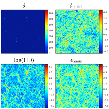
Figure 1 shows a slice of the Millennium Simulation density field (MS; Springel et al., 2005). The bottom panels show $\log(1+\delta)$, as well as a Gaussianized $\delta_{\rm Gauss}$, in which the ranking of cell densities is preserved, but they are mapped to a Gaussian probability density function (PDF). (‘log’ denotes the natural logarithm.) The bottom panels show more structure than the $\delta$ panel, which is why simulation visualizations often use logarithmic color tables. Figure 2 shows the high non-Gaussianity of the $\delta$ PDF compared to the $\log(1+\delta)$ PDF.

Figure 1.— Dark matter density in a slice 2 $h^{-1}$ Mpc thick and 250 $h^{-1}$ Mpc on a side in the Millennium simulation. $\delta$ is the overdensity at $z=0$. $\delta_{\rm init}$ is at $z=127$, scaled to have the same minimum as $\log(1+\delta)$, the natural logarithm of the density at $z=0$. The Gaussianized density $\delta_{\rm Gauss}$, at $z=0$, preserves the ranking of cell densities but imposes a Gaussian PDF with ${\rm Var}(\delta_{\rm Gauss})={\rm Var}[\log(1+\delta)]$. Particular structures at $z=0$ and $z=127$ disagree because of drift as the simulation progresses. See http://skysrv.pha.jhu.edu/~neyrinck/sonifylss.html for sounds representing these panels. The similarity in the sounds (except $\delta$’s) suggests a similarity in their power spectra.

Figure 2.— PDF’s of $\delta$ and $\log(1+\delta)$ measured in $2$- $h^{-1}$ Mpc cells in the Millennium simulation at $z=0$. Each distribution has been calibrated to have standard deviation 1.

All that is visible in the $\delta$ panel is a handful of discrete peaks (halos). This suggests why the standard power spectrum, $P_{\delta}$, is so sensitive to fluctuations in the halo population, and also suggests why the halo model successfully describes $P_{\delta}$. The other panels contain obvious filamentary structure, which we suspect the halo model would have more difficulty describing.

There are several reasons to use the log transform, despite the slight non-lognormality of the density PDF (Colombi, 1994). The lognormal distribution is simple; its use in galaxy number density PDF’s dates back to Hubble (1934). The log transform is easily reversible, and thus preserves pixel-by-pixel information. Coles & Jones (1991) showed that a lognormal density PDF emerges if peculiar velocities are assumed to grow according to linear theory, and showed that a lognormal density PDF can explain many features observed in our Universe.

In Schrödinger perturbation theory (SPT; Szapudi & Kaiser, 2003), $A=\log(1+\delta)/2$ is a natural density variable. In determining the variance of $\delta$, tree-level SPT in $A$ captures most of the higher-order loop corrections in standard perturbation theory. This suggests that the power spectrum of the log-mapped density could pull in information from higher-order statistics of $\delta$.

Another motivation for using the log transform is to make the power spectrum more suited to describe the density field. The power spectrum contains all the cosmological information in the Gaussian initial conditions; all higher moments are zero. The density field is statistically invariant under translations and rotations at all epochs. Initially, there is also a symmetry between underdense and overdense regions, related to the initial Gaussianity of the density PDF. At late times, this symmetry is broken, and high overdensities receive perhaps undue weight in measurement of the power spectrum. In this paper, we test the hypothesis that restoring the Gaussianity of the density PDF restores some information to the power spectrum.

2. Power spectrum nonlinearities

We measure nonlinearities in power spectra of the log-density ($P_{\log(1+\delta)}$) and the Gaussianized overdensity ($P_{\rm Gauss}$) using the dark-matter density field from the 500  $h^{-1}$ Mpc $\Lambda$CDM Millennium simulation (MS). We use publicly available time snapshots of the density measured with a nearest-grid-point (NGP) method on a 256³ grid. On this mesh, the shot noise is negligible; there is a mean of 600 and minimum of 6 particles per grid cell.

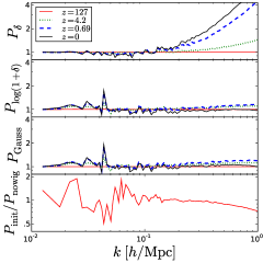
Figure 3 compares the distortion gravitational evolution imparts to various power spectra in the MS. We show the ratio of each power spectrum to the initial-conditions ($z=127$) power spectrum, dividing by factors to line up the power spectra in the lowest-$k$ bin. Also shown are the fluctuations of the initial power spectrum with the same binning, dividing by the no-wiggle power spectrum of Eisenstein & Hu (1998). We do not correct for the NGP pixel window function; for example, this causes the small-scale downturn in the bottom panel. We cut the plot slightly before the Nyquist wavenumber ($k=1.6$ $h$ Mpc^-1), but effects from the NGP assignment may persist at the smallest scales plotted. However, these effects should be mild for the ratios of two similar power spectra, i.e. in the $P_{\log(1+\delta)}$ and $P_{\rm Gauss}$ panels.

Figure 3.— The top 3 panels show the ratios of $P_{\delta}$, $P_{\log(1+\delta)}$, and $P_{\rm Gauss}$ to the initial power spectrum at various redshifts of the Millennium simulation. We apply a multiplicative factor to each curve to line up the power spectra in the lowest-$k$ bin. The bottom panel shows the level of fluctuation in the initial power spectrum using the same bins, relative to a no-wiggle power spectrum.

Both $P_{\log(1+\delta)}$ and $P_{\rm Gauss}$ experience minimal nonlinearities compared to the standard power spectrum $P_{\delta}$, to the extent that we conjecture that they trace the linear power spectrum itself well into the nonlinear regime. Possibly, a different transformation than a logarithm could give a better estimator of the linear power spectrum, but the similarity of $P_{\log(1+\delta)}$ and $P_{\rm Gauss}$ to each other suggests that $P_{\log(1+\delta)}$ is close to optimal already.

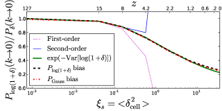
As structure develops, a multiplicative bias grows between $P_{\log(1+\delta)}$ and $P_{\delta}$ on large scales, shown in Figure 4 for several redshifts of the MS. This bias depends on the variance of cell densities, and thus on the cell size used to sample the density field.

Figure 4.— The large-scale biases $P_{\log(1+\delta)}$/$P_{\delta}$ and $P_{\rm Gauss}$/$P_{\delta}$ in the Millennium simulation sampled on a $256^{3}$ grid at various redshifts, measured using the lowest-$k$ bin. Also shown are a few analytic approximations, as given in the Appendix. The result in Eq. (1) traces each bias almost perfectly through $\left\langle{\delta_{\rm cell}^{2}}\right\rangle\approx 7$.

In the Appendix, we estimate the large-scale bias between $P_{\log(1+\delta)}$ and $P_{\delta}$ analytically, both perturbatively (assuming small fluctuations) and non-perturbatively (assuming a lognormal density PDF). Figure 4 shows the performance of these bias approximations. The non-perturbative result,

$$\lim_{k\to 0}\frac{P_{\log(1+\delta)}(k)}{P_{\delta}(k)}=e^{-{\rm Var}[\log(1+\delta_{\rm cell})]},$$ (1)

works almost perfectly through $\left\langle{\delta_{\rm cell}^{2}}\right\rangle\approx 7$. For the MS at this cell size, this occurs at $z=1.2$. At lower $z$, presumably, the density becomes insufficiently lognormal for the calculation to work perfectly. The perturbative results, given in the Appendix, work for $\left\langle{\delta_{\rm cell}^{2}}\right\rangle\ll 1$, as expected. We use perturbation theory (e.g., Bernardeau et al., 2002) on a linear power spectrum from camb (Lewis et al., 2000) to calculate the cumulants in the Appendix. The radius of the top-hat filter we used is that of a sphere with the volume of a grid cell. The bias is almost identical for $P_{\rm Gauss}$, if ${\rm Var}(\delta_{\rm Gauss})$ is set to ${\rm Var}[\log(1+\delta)]$.

3. Information content

We compare the information contents of $P_{\log(1+\delta)}$ and $P_{\delta}$ using the signal-to-noise (S/N; Takahashi et al., 2009), the Fisher information (Fisher, 1935; Tegmark et al., 1997) about the mean of a power spectrum itself. The S/N in a power spectrum over a range of bins $\mathcal{R}$ is defined as

$$F(\mathcal{R})=\sum_{i,j\in\mathcal{R}}(\textbf{{C}}_{\mathcal{R}}^{-1})_{ij}.$$ (2)

$\textbf{{C}}_{\mathcal{R}}$ is the covariance matrix of the power spectrum in bins, $C_{ij}=\left\langle{(P_{i}-\bar{P_{i}})(P_{j}-\bar{P_{j}})}\right\rangle/(\bar{P_{i}}\bar{P_{j}})$, not to be confused with the cumulants in the Appendix. Fisher information usually references a set of cosmological parameters, but an analysis of how $P_{\log(1+\delta)}$ varies with cosmological parameters is beyond the scope of this paper.

To measure the covariance matrices, we subject the MS to 248 different large-wavelength sinusoidal weightings that estimate the covariance in a single cubic simulation (Hamilton et al., 2006). This includes higher-order weightings than the 52 they recommend, reducing the noise somewhat, but increasing the minimum usable $k\in\mathcal{R}$. For $\bar{P_{i}}$, we use the power spectrum of the unweighted density. For $P_{\log(1+\delta)}$, we apply the weightings to $\log(1+\delta)-\left\langle{\log(1+\delta)}\right\rangle$, subtracting off the mean because the weightings can cause a spike in the power spectrum if the mean is nonzero.

Figure 5.— A comparison of the signal-to-noise for different power spectra at $z=0$, 1.2 and 127. Solid, dashed, and dotted curves show S/N in $P_{\delta}$, $P_{\log(1+\delta)}$, and $P_{\rm Gauss}$. The bold black curves use a degraded $128^{3}$ (from $256^{3}$) grid. At left, S/N are at $z=0$; the right panel also shows S/N at $z=1.2$. The $P_{\delta,\,{\rm global}\,\bar{\rho}}$ curve shows S/N for $P_{\delta}$ if the global instead of local mean density is used to estimate $\delta$ for each weighting.

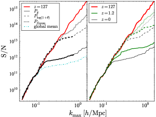
Figure 5 shows S/N for various power spectra. The smallest $k\in\mathcal{R}$ is fixed at the smallest $k$ not directly affected by weightings, and we vary the maximum $k_{\rm max}$. On linear scales, S/N $\propto k_{\rm max}^{3}$, proportional to the number of modes. We plot the S/N to the Nyquist wavenumber, because results for a downgraded $128^{3}$ grid were nearly identical to the $256^{3}$ results up to the $128^{3}$ Nyquist wavenumber. Still, features at $k_{\rm max}\approx 1$ $h$ Mpc^-1 should be interpreted cautiously. For $P_{\delta,\,{\rm global}\,\bar{\rho}}$, the mean density $\bar{\rho}$ used in $\delta=\rho/\bar{\rho}-1$ is the global mean of the simulation, while for $P_{\delta}$, the ‘local’ mean density is used, i.e. $\left\langle{\rho({\mbox{\boldmath$r$}})w({\mbox{\boldmath$r$}})^{2}}\right\rangle$, where $w({\mbox{\boldmath$r$}})$ is one of the 248 weighting functions. Using the local mean actually boosts the S/N somewhat in $P_{\delta}$, because generally, denser regions have higher translinear power.

The S/N in $P_{\log(1+\delta)}$ continues to grow with $k_{\rm max}^{3}$ for an extra factor of 2-3 beyond where the S/N in $P_{\delta}$ turns over, giving a factor of $\sim 10$ S/N increase on small scales. The S/N in $P_{\rm Gauss}$ reaches a factor of 2 even higher. The global vs. local mean-density issue does not apply to $P_{\rm Gauss}$ and $P_{\log(1+\delta)}$.

4. Conclusion

We find that the power spectrum of the log of the matter density, $P_{\log(1+\delta)}$, and the power spectrum of $\delta$ after Gaussianizing its PDF, $P_{\rm Gauss}$, suffer dramatically smaller nonlinearities than the standard matter power spectrum $P_{\delta}$ on translinear scales at all redshifts tested. This is true for both the mean of the power spectrum and its covariance, as we measure from the high-resolution Millennium simulation (MS). Not only do $P_{\log(1+\delta)}$ and $P_{\rm Gauss}$ seem to trace the linear power spectrum to nearly $k=1$ $h$ Mpc^-1, but they respectively contain factors of 10 and 20 higher signal-to-noise than $P_{\delta}$ at $z=0$.

To constrain cosmology, it is necessary to study how $P_{\log(1+\delta)}$ varies with cosmological parameters. Much current large-scale-structure research is focused on baryon acoustic oscillations (BAO’s), so a major issue to investigate is the degree of BAO attenuation in $P_{\log(1+\delta)}$. The MS by itself is too small to provide an adequate answer to this question. BAO detection would likely benefit from the lack of nonlinearities in $P_{\log(1+\delta)}$ on BAO scales, although the BAO’s in $P_{\log(1+\delta)}$ might experience some smearing as in $P_{\delta}$. These results are also encouraging for non-BAO large-scale-structure cosmology, since they imply a significantly larger range of scales over which the linear power spectrum can be accessed.

It is also necessary to investigate the effects of redshift space distortions, shot noise, and galaxy bias on $P_{\log(1+\delta)}$. Shot noise could be a significant issue in realistic surveys because accurately constructing the $\log(1+\delta)$ and $\delta_{\rm Gauss}$ fields requires knowledge of the density even in voids. It could be that $P_{\log(1+\delta)}$ has low sensitivity to the accuracy of densities estimated in voids, but it is likely that adaptive density kernels or tessellation methods (e.g., van de Weygaert & Schaap, 2009) will be needed to achieve substantial information gains with $P_{\log(1+\delta)}$ over $P_{\delta}$. The issue of galaxy bias could actually be a positive feature of $P_{\log(1+\delta)}$ even on linear scales, since at least in the limit of large $\delta\approx\delta+1$, $P_{\log(1+\delta)}$ is insensitive to linear galaxy bias. Although $P_{\rm Gauss}$ outperforms $P_{\log(1+\delta)}$ in our idealized simulation, it remains to be seen what the optimal transform is in the face of shot noise and other observational issues.

It is reassuring to find that at least in principle, much information that gravity seemed to have unfairly stripped from the matter power spectrum on translinear scales is retrievable with a simple transformation on the density field. A log transform could also prove useful for other statistics, such as estimators of primordial non-Gaussianity from large-scale structure.

Appendix A Analytic estimates of the log-density power spectrum bias

The power spectrum $P_{A}$ of the log-density $A=\log(1+\delta)$ [for simplicity, $A$ is twice the quantity defined by Szapudi & Kaiser (2003)] is generally biased on large scales relative to the standard $P_{\delta}$. We can calculate the moments of the $A$ field with brute-force perturbation theory for small $\delta$, and express them in terms of the connected moments of $\delta$.

Since $A$ is not a zero-mean field, we start with the mean for completeness. Expanding the logarithm:

$$\left\langle{A}\right\rangle=\left\langle{\delta-\frac{\delta^{2}}{2}+\frac{\delta^{3}}{3}-\frac{\delta^{4}}{4}\pm\ldots}\right\rangle=\frac{\xi_{s}}{2}+\frac{S_{3}\xi_{s}^{2}}{3}+\frac{3\xi_{s}^{2}}{4}+{\cal O}(\xi_{s}^{3}),$$ (A1)

where $\xi_{s}$ is the average of the correlation function within grid cells (i.e. the variance of cell densities). The main subtlety of the calculation is to take into account the connectedness of the moments (e.g., Szapudi, 2009, for detailed explanation). The skewness $S_{3}$ and the cumulants $C_{N,M}$ (below) are defined by $S_{3}=\frac{\left\langle{\delta^{3}}\right\rangle_{\rm c}}{\left\langle{\delta^{2}}\right\rangle^{2}}$ and $C_{N,M}=\frac{\left\langle{\delta_{1}^{N}\delta_{2}^{M}}\right\rangle_{\rm c}}{\left\langle{\delta_{1}\delta_{2}}\right\rangle\left\langle{\delta^{2}}\right\rangle^{M+N-2}}$.

The calculation of $\left\langle{A_{1}A_{2}}\right\rangle$ is analogous to the above. Expanding the logarithm, and expressing the results in terms of connected moments:

$$\left\langle{A_{1}A_{2}}\right\rangle=\frac{\xi_{s}^{2}}{4}+\xi_{\ell}\left[1+\xi_{s}\left(2-C_{1,2}\right)+\xi_{s}^{2}\left(7-2S_{3}-4C_{1,2}+\frac{2C_{1,3}}{3}+\frac{C_{2,2}}{4}\right)\right]+{\cal O}(\xi_{s}^{3}).$$ (A2)

The DC term $\xi_{s}^{2}/4$ affects the two-point correlation function, but not the power spectrum. The large-scale power spectrum bias is the coefficient of $\xi_{\ell}$, the large-scale correlation function subtracting off contributions from $\xi_{s}$.

For the non-perturbative calculation, we introduce $D=A-\left\langle{A}\right\rangle$. $\left\langle{\delta}\right\rangle=0$, so $\left\langle{e^{D+\left\langle{A}\right\rangle}}\right\rangle=1$. Using the connected moment theorem (Wilf, 1994; Szalay, 1988; Szapudi & Szalay, 1993), and assuming $D$ to be Gaussian, making all of its higher-than-second-order connected moments vanish, we obtain

$$1+\xi_{\ell}=\left\langle{e^{D_{1}}e^{D_{2}}}\right\rangle=e^{\left\langle{D_{1}D_{2}}\right\rangle+\left\langle{D^{2}}\right\rangle}.$$ (A3)

Using $\exp{\left\langle{D_{1}D_{2}}\right\rangle}\simeq 1+\left\langle{D_{1}D_{2}}\right\rangle$, and Fourier transforming, yields the non-perturbative shift of $\exp{\left\langle{D^{2}}\right\rangle}$ in Eq. (1).

References

- Bernardeau et al. (2002) Bernardeau, F., Colombi, S., Gaztañaga, E., & Scoccimarro, R. 2002, Phys. Rep., 367, 1
- Coles & Jones (1991) Coles, P., & Jones, B. 1991, MNRAS, 248, 1
- Colombi (1994) Colombi, S. 1994, ApJ, 435, 536
- Cooray & Hu (2001) Cooray, A., & Hu, W. 2001, ApJ, 554, 56
- Cooray & Sheth (2002) Cooray, A., & Sheth, R. 2002, Phys. Rep., 372, 1, arXiv:astro-ph/0206508
- Eisenstein & Hu (1998) Eisenstein, D. J., & Hu, W. 1998, ApJ, 496, 605
- Fisher (1935) Fisher, R. A. 1935, J. Roy. Stat. Soc., 98, 39
- Hamilton et al. (2006) Hamilton, A. J. S., Rimes, C. D., & Scoccimarro, R. 2006, MNRAS, 371, 1188
- Hubble (1934) Hubble, E. 1934, ApJ, 79, 8
- Lee & Pen (2008) Lee, J., & Pen, U.-L. 2008, ApJ, 686, L1
- Lewis et al. (2000) Lewis, A., Challinor, A., & Lasenby, A. 2000, ApJ, 538, 473, http://www.camb.info/
- Meiksin & White (1999) Meiksin, A., & White, M. 1999, MNRAS, 308, 1179
- Neyrinck & Szapudi (2007) Neyrinck, M. C., & Szapudi, I. 2007, MNRAS, 375, L51
- Neyrinck et al. (2006) Neyrinck, M. C., Szapudi, I., & Rimes, C. D. 2006, MNRAS, 370, L66
- Pope et al. (2004) Pope, A. C. et al. 2004, ApJ, 607, 655
- Rimes & Hamilton (2005) Rimes, C. D., & Hamilton, A. J. S. 2005, MNRAS, 360, L82
- Rimes & Hamilton (2006) ——. 2006, MNRAS, 371, 1205
- Scoccimarro et al. (1999) Scoccimarro, R., Zaldarriaga, M., & Hui, L. 1999, ApJ, 527, 1
- Springel et al. (2005) Springel, V. et al. 2005, Nature, 435, 629
- Szalay (1988) Szalay, A. S. 1988, ApJ, 333, 21
- Szapudi (2009) Szapudi, I. 2009, in Lecture Notes in Physics, Vol. 665, Data Analysis in Cosmology, ed. V. Martínez, E. Saar, E. Martínez-Gonzáles, & M.-J. Pons-Bordería (Berlin: Springer), 457–489, arXiv:astro-ph/0505391
- Szapudi & Kaiser (2003) Szapudi, I., & Kaiser, N. 2003, ApJ, 583, L1
- Szapudi & Szalay (1993) Szapudi, I., & Szalay, A. S. 1993, ApJ, 408, 43
- Takahashi et al. (2009) Takahashi, R. et al. 2009, ApJ, sumbitted, arXiv:0902.0371
- Tegmark et al. (2006) Tegmark, M. et al. 2006, Phys. Rev. D, 74, 123507
- Tegmark et al. (1997) Tegmark, M., Taylor, A. N., & Heavens, A. F. 1997, ApJ, 480, 22
- van de Weygaert & Schaap (2009) van de Weygaert, R., & Schaap, W. 2009, in Lecture Notes in Physics, Vol. 665, Data Analysis in Cosmology, ed. V. Martínez, E. Saar, E. Martínez-Gonzáles, & M.-J. Pons-Bordería (Berlin: Springer), 291–413, arXiv:0708.1441
-
Wilf (1994)
Wilf, H. S. 1994, generatingfunctionology, 2nd edn. (Academic Press),
http://www.math.upenn.edu/~wilf/DownldGF.html