Gamma-ray background anisotropy from galactic dark matter substructure
Abstract
Dark matter annihilation in galactic substructure would imprint characteristic angular signatures on the all-sky map of the diffuse gamma-ray background. We study the gamma-ray background anisotropy due to the subhalos and discuss detectability at Fermi Gamma-ray Space Telescope. In contrast to earlier work that relies on simulated all-sky maps, we derive analytic formulae that enable to directly compute the angular power spectrum, given parameters of subhalos such as mass function and radial profile of gamma-ray luminosity. As our fiducial subhalo models, we adopt mass spectrum, subhalos radial distribution suppressed towards the galactic center, and luminosity profile of each subhalo dominated by its smooth component. We find that, for multipole regime corresponding to , the angular power spectrum is dominated by a noise-like term, with suppression due to internal structure of relevant subhalos. If the mass spectrum extends down to Earth-mass scale, then the subhalos would be detected in the anisotropy with Fermi at angular scales of 10∘, if their contribution to the gamma-ray background is larger than 20%. If the minimum mass is around , on the other hand, the relevant angular scale for detection is 1∘, and the anisotropy detection requires that the subhalo contribution to the gamma-ray background intensity is only 4%. These can be achieved with a modest boost for particle physics parameters. We also find that the anisotropy analysis could be a more sensitive probe for the subhalos than individual detection. We also study dependence on model parameters, where we reach the similar conclusions for all the models investigated. The analytic approach should be very useful when Fermi data are analyzed and the obtained angular power spectrum is interpreted in terms of subhalo models.
pacs:
95.35.+d, 95.85.Pw, 98.35.Gi, 98.70.VcI Introduction
Modern astrophysical and cosmological measurements strongly support existence of nonbaryonic dark matter. Although the true identity of dark matter is unknown observationally and experimentally, there are several well-motivated particle-physics models that provide a candidate particle for dark matter. Weakly interacting massive particles (WIMPs) such as supersymmetric neutralinos are perhaps the most popular candidate Jungman1996 ; Hooper2007a . As they interact with themselves as well as standard-model particles, many experiments are being carried out to look for signatures of scattering of WIMPs off nuclei in underground detectors and of self-annihilation of WIMP particles in dark matter halos Bertone2005 .
Recently launched Fermi Gamma-ray Space Telescope Atwood2009 features promising capability to detect gamma rays from WIMP annihilation in the right energy range Baltz2008 . In addition, recent numerical simulations find that dark matter in a host halo is distributed in clumpy substructure (subhalos) Moore1999 ; Klypin1999 ; Diemand2005 ; Diemand2006 whose masses range quite widely, potentially down to Earth mass Hofmann2001 ; Green2005 ; Loeb2005 ; Profumo2006 ; Bertschinger2006 . This feature is encouraging because annihilation probability is proportional to density squared, and thus the significant clumpiness boosts the gamma-ray yields. Several avenues have been proposed for Fermi to look for annihilation gamma rays: galactic center Berezinsky1994 ; Bergstrom1998 ; Cesarini2004 ; Fornengo2004 ; Dodelson2008 , relatively massive substructure often associated with dwarf galaxies Bergstrom1999 ; Calcaneo-Roldan2000 ; Tasitsiomi2002 ; Stoehr2003 ; Evans2004 ; Aloisio2004 ; Koushiappas2004 ; Diemand2007a ; Strigari2008 ; Pieri2008 ; Kuhlen2008 ; Martinez2009 , proper motions of nearby small subhalos Koushiappas2006 ; Ando2008 , diffuse gamma-ray background Bergstrom2001 ; Ullio2002 ; Taylor2003 ; Elsaesser2005 ; Ando2005 ; Oda2005 ; Horiuchi2006 , etc.
There is an increasing interest in statistical analysis of the all-sky map of the gamma-ray background obtained with Fermi in the near future. References Ando2006 ; Ando2007a computed angular power spectrum of the gamma-ray background from annihilation in extragalactic dark matter halos, and showed that the signature would be different from that of ordinary astrophysical sources (see also, Refs. Cuoco2007 ; Cuoco2008 ; Zhang2008 ; Taoso2008 ). The same approach has been applied to signals from substructure in the galactic halo Siegal-Gaskins2008 ; Fornasa2009 . This is indeed important, because the galactic substructure typically gives a larger contribution to the diffuse gamma-ray background than extragalactic halos do Fornasa2009 ; Hooper2007b ; Yuksel2007 . In Refs. Siegal-Gaskins2008 ; Fornasa2009 , first the all-sky gamma-ray map was simulated from sets of subhalo models, and then the map was analyzed to obtain the angular power spectrum. In addition, one-point probability distribution function of the gamma-ray flux has also been studied Lee2008 ; Dodelson2009 .
In this paper, we revisit the gamma-ray background anisotropy from dark matter annihilation in the galactic subhalos. In contrast to the earlier works Siegal-Gaskins2008 ; Fornasa2009 that heavily relied on mock gamma-ray maps generated from subhalo models, we develop an analytic approach to compute the angular power spectrum directly. This way, we are able to calculate the angular power spectrum easily and more quickly, if we specify some input parameters and characteristics of galactic subhalos. This would be in particular useful when we have results of actual Fermi data analysis, and try to give physical interpretation for them.
We find that the angular power spectrum is divided into two parts: one depending on (ensemble-averaged) distribution of subhalos in a host (“two-subhalo” term, ), and the other depending on the emissivity profile of single subhalos as well as the number of subhalos significantly contributing to the background intensity (“one-subhalo” term, ). The latter would be shot noise if the subhalos were completely point sources, but Fermi will be able to see deviations from the shot noise due to the angular extension of the relevant subhalos. Using the latest subhalo models following recent numerical simulations, we give predictions for the angular power spectrum, and show that the multipole range would be a favorable window for anisotropy detection. We also discuss the detectability of the angular power spectrum from subhalos with Fermi, which turns out to be promising, potentially better than the detection of subhalos as identified gamma-ray sources.
This paper is organized as follows. In Sec. II, we give formulation for angular power spectrum as well as mean intensity of the gamma-ray background. These formulae derived are applied to several subhalo models in the subsequent sections. In Sec. III, we study a simple case in which all the subhalos are assumed to be a point-like gamma-ray emitters. The case of extended subhalos is addressed in Sec. IV, where we also discuss detectability with Fermi. We close this paper by discussing the results in Sec. V and by giving concluding remarks in Sec. VI.
II Formulation
II.1 Relevant quantities of subhalos
We assume that a fraction of the mass of the galactic halo is in the form of subhalos, and is distributed as a smooth halo. For the density profile of the Milky-Way dark matter halo, we adopt a spherically symmetric Navarro-Frenk-White (NFW) profile Navarro1997 :
| (1) |
where is the galactocentric radius, and are the scale radius and scale density of the Milky-Way halo, respectively. This profile extends up to a virial radius , and an enclosed mass within this radius is defined as a virial mass . We use the following values for these parameters: kpc, kpc-3, kpc, and Klypin2002 .
As subhalo number density per unit mass range, we define a subhalo mass function, , and upper and lower limits of the function by and , respectively. Numerical simulations imply that the shape of mass distribution follows typically a power law, which is close to , i.e., the same amount of subhalo masses per decade Ghigna2000 ; DeLucia2004 ; Gao2004 ; Shaw2007 ; Diemand2007b . We also assume that there is a one-to-one relation between subhalo masses and luminosities , and therefore, the luminosity function is written as . The upper and lower limits on the luminosity function are then given by and , respectively. After integrating the mass (luminosity) function over mass (luminosity), we obtain the number density of subhalos .
We assume that each subhalo has extended, isotropic emissivity profile around its center (we call this “seed” position), , with the profile function normalized so that it gives unity after volume integration. We also define the Fourier transform of : , where is the wave number.
II.2 Gamma-ray intensity from subhalos
We label positions of seed of a subhalo by , and its luminosity and mass by and , respectively. With these definitions, the gamma-ray intensity towards a direction is given by the line-of-sight integration () of the emissivity:
| (2) | |||||
for one realization of the universe, where is the -dimensional delta function. Throughout this paper, we define the intensity as a number of gamma-ray photons per unit area, time, and solid angle, and the luminosity as a number of photons emitted per unit time. We also assume GeV as a targeted gamma-ray energy.
We now take ensemble average over infinite number of realizations of the universe. The discrete source distribution then becomes continuous function; i.e.,
| (3) |
where the bracket represents the ensemble average. Using these in Eq. (2), an ensemble-averaged intensity is
| (4) | |||||
We further assume that spatial extension of each subhalo is much smaller than a scale on which subhalo distribution significantly changes. With this reasonable assumption, we could take the luminosity function out of the volume integral by taking , since it is a slowly varying function of . As the integration of over simply becomes unity, the ensemble average of intensity is
| (5) |
where we specified upper and lower limits of the integrals. Galactocentric radius corresponding to (appearing as index of luminosity function) is obtained through the relation: , where kpc is the galactocentric radius of the solar system and is the angle between and the direction to the galactic center. We obtain the lower limit of the -integral by the detection criterion with the flux sensitivity of Fermi (typically cm-2 s-1 for photons that we consider). By setting this, we do not add contributions from subhalos bright enough to be identified as individual sources. The upper limit corresponds to through the relation .
By further averaging over directions , we obtain a mean gamma-ray intensity
| (6) | |||||
where we represent quantities averaged over by putting a horizontal line on top of them, and is the solid angle of the sky over which the averages are taken. In the second equality, we approximate , as ; since is now independent of , we could perform the angle average of before integrating over and .
The expected number of subhalos that would be detected as individual sources from is then
| (7) |
as we count sources close enough to give a flux larger than ; i.e., .
II.3 Angular power spectrum of gamma-ray background from subhalos
We decompose the gamma-ray intensity map with spherical harmonics:
| (8) |
Therefore (dimensionless) expansion coefficients are obtained from the intensity map through the inverse relation,
| (9) | |||||
where , and the second equality holds except for monopole (i.e., for ).
From Eq. (9), we have, for ,
| (10) | |||||
where . Thus, we want to evaluate , which now through Eq. (2) depends on
Since and represent positions of the subhalo seeds, the first term correlates positions and luminosities of two distinct subhalos (two-subhalo term). Here is the intrinsic two-point correlation function of the subhalo seeds. This two-subhalo term corresponds to a “one-halo term” of the halo model Seljak2000 , which is proportional to and gives dominant contribution to the galaxy power spectrum at scales smaller than the virial radius of halos. Although in the halo model one often discusses galaxy power spectrum and stands for the total number of galaxies in the host halo, exactly the same argument can be applied to the subhalo power spectrum, and therefore, is regarded as number of subhalos instead. The correlation function is related to via , and numerical simulations show that is very close to 1, if the host is massive enough to contain large number of galaxies (subhalos), Kravtsov2004 ; Zentner2005 , the case we consider here. The second term of Eq. (LABEL:eq:one_and_two-subhalo_terms), on the other hand, represents the case of one identical halo where and (one-subhalo term). Therefore, one-subhalo and two-subhalo terms of are
| (12) | |||||
| (13) |
We work on to further simplify Eq. (12). First, we again take the luminosity function out of -integral with the index , as its change on subhalo scales is moderate. Then, we take Fourier transforms of : . With this, -integral gives the delta function that collapses one of the -integrals, leaving a common wave number. Finally, we use the small-separation approximation (e.g., Peebles1980 ), where we take , , , , and instead of , , , and ; these quantities are related via , , and . This small-angle approximation is valid because, for one-subhalo term, we correlate two points in identical subhalos, and their angular diameter is very small, thus . We now have
| (14) | |||||
Angular power spectrum is given by
| (15) |
Using Eq. (10) as well as a relation between spherical harmonics and Legendre polynomials, i.e., Eq. (46.7) of Ref. Peebles1980 , we have
| (16) | |||||
In the second equality, we used an approximation valid for small and large ’s, where is the Legendre polynomials and is the Bessel function of zeroth order. In the last equality, angle integral between and was recovered (see, e.g., Ref. Peebles1980 ). This approximation is again particularly good for small angular scales (large ’s), where the one-subhalo term would dominate. Now, it is possible to simplify the -integral of ; with Eq. (14), its relevant part is
| (17) | |||||
where in the first equality, we decomposed the wave number by the components parallel and perpendicular to , i.e., , and used .
To summarize, combining Eq. (16) with Eqs. (14) and (17) for the one-subhalo term, and with Eq. (13) for the two-subhalo term, the angular power spectrum of gamma-ray background from galactic subhalos is
| (18) | |||||
| (19) | |||||
| (20) | |||||
where in Eq. (19), we again performed solid-angle integral first, and used angle-averaged luminosity function in the integrand. We do not try to further simplify Eq. (20), as the two-subhalo term would be more important at large angular scales (as shown below), where the small-angle approximation is no longer valid.
III Results for point-like subhalos
In this and subsequent sections, we apply the formulae for angular power spectrum derived in the previous section to several subhalo models. Here, first, we consider simple models in which we regard all the subhalos as gamma-ray point sources, i.e., . Its Fourier transform is therefore , independently of wave number and mass. Then the one-subhalo term of the angular power spectrum [Eq. (19)] is independent of multipole , and reduces to the Poisson (shot) noise.
III.1 Models
Following results of recent numerical simulations, we adopt the power-law mass function, , and assume that mass distribution is independent of subhalo positions in the host; i.e.,
| (21) |
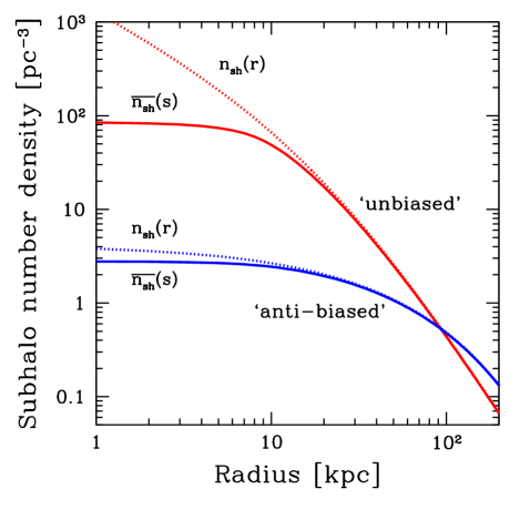
where we assumed and typical value for is about 2. For the subhalo number density , we adopt two different models. One is an “unbiased” model where the subhalo distribution follows the NFW density profile of the parent halo, . The other is an “anti-biased” model where the distribution is flatter than NFW profile and features a central core. For this model, we adopt the Einasto profile Einasto1969 , with parameters and , where is a radius within which the average density is 200 times the critical density (see Appendix A). The latter model takes into account the effect of gravitational tidal disruption of subhalos that is stronger and reduces the number of subhalos towards the central regions of the halo, and indeed is more likely to be the case according to numerical simulations Springel2008a (see also Refs. Nagai2005 ; Wetzel2008 ). Concrete expressions for for each case are summarized in Appendix A. Figure 1 shows the subhalo number densities , for both the unbiased and anti-biased distributions (dotted curves).
Figure 1 also shows the angle-averaged number density (solid). Note that unlike that is a function of galactocentric radius , is a function of distance from Earth . We adopt the same sky region over which we take the average as in Ref. Sreekumar1998 , where the analysis of the isotropic diffuse gamma-ray background was performed for the Energetic Gamma-Ray Experimental Telescope (EGRET); i.e., the galactic center ( and , where and are the galactic latitude and longitude, respectively) as well as the galactic plane () are masked, for which . As the galactic center is masked, is fairly flat within 10 kpc, beyond which it reaches regions where the density drops more rapidly , and it eventually becomes almost the same as .
We assume positive correlation between gamma-ray luminosity and mass, (). Then, the luminosity function is obtained by , which yields
| (22) |
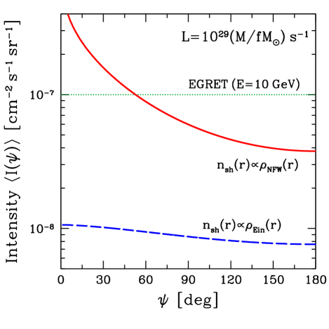
The absolute value of the luminosity, e.g., , can be kept arbitrary, because we are here interested in intensity fluctuation divided by the mean intensity, where the absolute value cancel out.111There is also an implicit dependence on it through the lower limit of -integral, , but it is very weak. Still we comment that in order to make the mean intensity as large as the observed value around 10 GeV with EGRET Sreekumar1998 , has to be no smaller than 10 s-1 if for the unbiased model Ando2008 ; Lee2008 ; for anti-biased model, on the other hand, this value has to be 7 times larger. In Fig. 2, we show as a function of , in the case of s-1 () for both the unbiased (solid) and anti-biased (dashed) models. For comparison, we also show the gamma-ray background intensity measured with EGRET for 10-GeV photons (dotted) Sreekumar1998 . The number of detectable subhalos and angle-averaged mean intensities for these models are , cm-2 s-1 sr-1 for the unbiased, and , cm-2 s-1 sr-1 for the anti-biased distribution.
III.2 Angular power spectrum
We now move on to the angular power spectrum, starting with the two-subhalo term [Eq. (20)], which would dominate for large angular scales. To evaluate , we use HEALPix222http://healpix.jpl.nasa.gov package Gorski2005 to generate and analyze the gamma-ray map, for which we used parameters and that correspond to pixel size of , small enough compared with angular resolution of Fermi, 0.1∘ for a 10-GeV photon. The resulting has a highly oscillatory feature as a function of , so we average over logarithmic bin for a given .
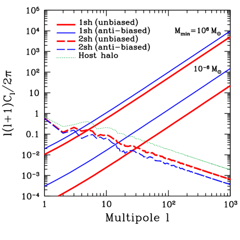
In Fig. 3, we show , for both the unbiased and anti-biased models (dashed curves), assuming . As expected, it becomes anisotropic for large angular scales and small multipole ranges. At smaller angular scales, where , the two-subhalo term becomes less important compared with the one-subhalo (Poisson) term for which as we see below. Therefore, in general, the two-subhalo term can be safely neglected for small angular scales. The difference between the unbiased and anti-biased distributions is not very large, a factor of two larger for the former. We also confirmed that the dependence on a chosen mask is weak.
There is also contribution to the gamma-ray background from a smoothly distributed dark matter component. Its emissivity profile is then proportional to as annihilation is a two-body process. The angular power spectrum from this smooth component can be also evaluated with Eq. (20), but by using line-of-sight integral of for , rather than of or as we see in, e.g., Eq. (5). Figure 3 also shows the angular power spectrum from the host-halo component (dotted). The tendency is the same as the two-subhalo terms, with amplitudes further larger by a factor of 3 than the unbiased subhalo distribution. Note that in this case, the mean intensity is evaluated assuming that only the smooth halo gives contribution to the gamma-ray background (i.e., no substructure). If we consider both the subhalos and smooth halo, the amplitude is reduced depending on contribution to the mean intensity from each component (see Sec. IV.2).
We now discuss the one-subhalo term . If all the subhalos are regarded as point sources, , becomes independent of , , where the Poisson-noise (shot or white-noise) term is given by
| (23) |
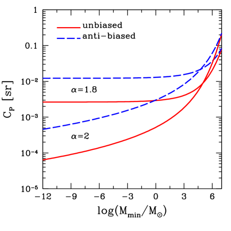
Its integrand depends on subhalo number density , whereas in the denominator appears and each depends on the subhalo density. Thus, roughly speaking, is inversely proportional to number of subhalos that give significant contribution to the mean intensity. In Fig. 3, we also show for the unbiased (thick-red) and anti-biased (thin-blue) distributions. By fixing the parameters , , and , we compare results for and . In the case of larger , the mean intensity is dominated by bright (massive), relatively rare subhalos. On the other hand, in the case of small , one includes fainter subhalos, which increases effective number of sources that contribute to the mean intensity and thus reduces . This trend is clearly seen in Fig. 3 and consistent with the earlier report in Ref. Siegal-Gaskins2008 . In Fig. 4, we plot as a function of for the unbiased and anti-biased distributions and for and 1.8. Here we rescaled such that contribution to it from the mass range of – is 0.125; by this, for instance, we get (0.15) for (1.8) and . When the luminosity function is biased towards high-luminosity range as in the case of , including smaller subhalos has less significant impact on the mean intensity. Therefore, the angular power spectrum is fairly flat for in this case.
IV Results for extended subhalo models
IV.1 Subhalo models
We move on to evaluating the angular power spectrum with more realistic models where angular extension of the gamma-ray intensity profile for each subhalo is taken into account. The models we use are the same as those given in Sec. III.1 except for the source extension as well as the luminosity-mass relation that then affects the luminosity function.
As the subhalos are in gravitational potential well of the host, they are subject to tidal disruption, and therefore, their outer regions are stripped away. The inner regions, on the other hand, are more resilient against such an effect. Hence it would be a good approximation to assume that the subhalo density profile is given by a truncated NFW profile:
| (24) |
where is a cutoff radius and this is typically much smaller than the virial radius. This has been studied extensively in Ref. Kazantzidis2004 (see also Refs. Stoehr2002 ; Hayashi2003 ; Penarrubia2008 ).
The gamma-ray luminosity is then given by
| (25) | |||||
where is thermally averaged annihilation cross section times relative velocity, is WIMP mass, and is number of gamma-ray photons emitted per annihilation. In the second equality we define
where we normalize each parameter with typical values often taken in the literature, and cm3 s-1 GeV-2. The value of is closely related to the relic density of dark matter as it determines the abundance of dark matter particles having survived pair annihilation in the early universe. For the supersymmetric neutralino, whose mass is around 100 GeV, cm3 s-1 is the canonical value Jungman1996 , while a wide range of parameter space is still allowed Bertone2005 . To obtain , we used the result of Ref. Bergstrom2001 , where the gamma-ray spectrum as a result of hadronization and decay of has been fitted with a simple formula. We also introduce additional boost factor due to internal structure in the subhalo (see below).
The luminosity also depends on the volume integral of the subhalo density squared , which is rewritten in terms of mass , scale radius , and “concentration” parameter of subhalos.333We note that concentration parameter is conventionally defined as a ratio of virial radius and scale radius. Here, we use the same terminology also for a different, albeit similar, quantity . Both and are functions of subhalo mass. In order to obtain values of these quantities for a given mass, we adopt scaling relations among various quantities found in the recent numerical simulations of Ref. Springel2008a . More specifically, we adopt the following empirical relations between , and : and , where is the maximum rotation velocity of the subhalo, is the radius at which the rotation curve hits the maximum, and is the Hubble constant. We here postulate that for most of the subhalos investigated in Ref. Springel2008a the density profile is well approximated by NFW within (i.e., ) and it is indeed the case for a sample of subhalos shown in Fig. 22 of Ref. Springel2008a . Therefore, we can use the relations between and for the NFW profile, and , to obtain and as a function of subhalo mass . Then finally, to get the cutoff radius , we require that the volume integral of Eq. (24) equals to . We find that the concentration parameter is a decreasing function of , but still larger than 2.163 (i.e., ) even at the resolution limit of the simulation, , confirming that this procedure gives consistent values for , , and . These empirical relations do not hold at lower mass regions. Therefore, we adopt two different approaches, one simply extrapolating the same relations down to Earth-mass scale , and the other assuming there is no contribution from subhalos less massive than .
Recent numerical simulations also tend to imply presence of internal structure within subhalos, i.e., “sub-subhalos.” If we include these sub-subhalos, both the subhalo luminosity and its spatial profile will change. For the former, it will give additional boost , for which we adopt (2) for (1.9 and 1.8) as it is weakly dependent on subhalo masses Kuhlen2008 . Hence, this effect on the angular power spectrum is expected to be rather minor. For the latter, on the other hand, the effect would be more prominent. If the luminosity is dominated by a sub-subhalo component, it would change the smooth density-squared intensity profile to the clumpy one that is close to proportionality with the density, i.e., . Although tidal disruption is likely to convert the sub-subhalo component into the smooth subhalo component without much changing luminosity from the latter Springel2008b , we still adopt this model regarding it as an extreme possibility. The Fourier transforms of the emissivity profile for both cases are summarized in Appendix B.
Considering all of the recent development summarized above, we here adopt as our fiducial subhalo model the following characteristics: (i) power-law mass function Springel2008a with maximum mass of ; (ii) anti-biased subhalo distribution in the galactic halo, ; (iii) scale radius and concentration parameter for subhalos as a function of mass obtained from the empirical relations in Ref. Springel2008a ; (iv) subhalo luminosity obtained with canonical values of the particle-physics parameters, , and the additional subhalo boost of ; and (v) emissivity profile of each subhalo dominated by its smooth component, . We refer to this fiducial set of parameters as the model “A.” However, we still do not know if the phenomenological relations visited in (iii) above as well as the mass function still hold at the mass scales smaller than the current resolution limit. Therefore, we adopt two minimum mass scales: for the model A1 and for the model A2. In Sec. IV.2, we extensively discuss the angular power spectrum for these fiducial models, and in Sec. IV.3 we study dependence of results on chosen models and parameter values.
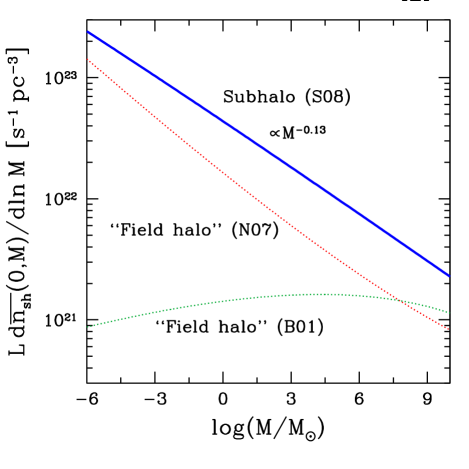
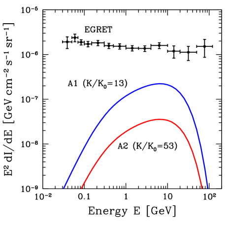
Before closing this subsection, in Fig. 5, we show the luminosity-weighted mass function, at obtained for the fiducial models. This quantity tells us which mass range contributes to the gamma-ray intensity the most [see Eq. (6)]. The fiducial subhalo model is labeled as S08 according to the reference on which this model is based (Ref. Springel2008a ), and this function is well fitted by the scaling (). Therefore, the smaller subhalos give more important contribution to the mean intensity. In the same figure, we also show results based on other mass-concentration relations given in Refs. Bullock2001 (B01; see also Refs. Kuhlen2005 ; Maccio2007 ) and Neto2007 (N07). These are, however, for field halos that are not fell in potential well of another larger halo, and hence, their mass is virial mass and the concentration parameter is defined as the ratio of virial radius and scale radius as conventionally done. These models shown in Fig. 5 thus tell us what the luminosity-weighted mass function would be if there were no tidal forces acting on subhalos. Note also that these concentration models are calibrated at even larger scales, such as of galaxies and galaxy clusters, and the results shown here is based on even more violent extrapolation. Nevertheless, it is shown that the subhalos are more luminous than the field halos of equal mass, and this difference might be as large as two orders of magnitude. Qualitatively, this difference can be explained as follows. Tidal force strips the outer region of subhalos away, but the central region is more strongly bound. This will reduce the mass of the subhalos significantly but hardly affect the gamma-ray luminosity that is proportional to the density squared. Finally, in Fig. 6, we show energy spectrum of the mean intensity for the models A1 and A2, compared with the EGRET data Sreekumar1998 . These subhalo models are boosted by a factor of (A1) and 53 (A2), with which associated anisotropies would be detected (see discussion in the next subsection).
IV.2 Results for the fiducial model and detectability with Fermi
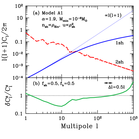
In Fig. 7(a), we show for the fiducial model A1. The two-subhalo term [Eq. (20) with ] is much smaller than the one-subhalo term [Eq. (19)] for large multipole ranges. For comparison, we also show the Poisson noise [Eq. (23)] evaluated for the same model, which would be realized if all the subhalos were to be gamma-ray point sources. As expected, the power spectrum is more suppressed at smaller angular scales (higher multipoles) compared with the noise-like spectrum. This means that internal structure of the subhalos should be probed with this analysis.
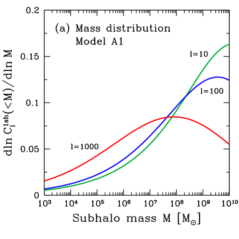
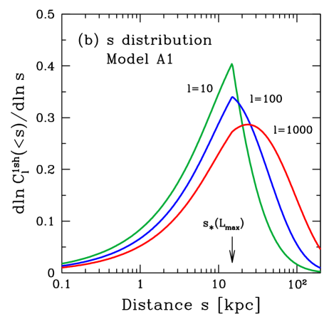
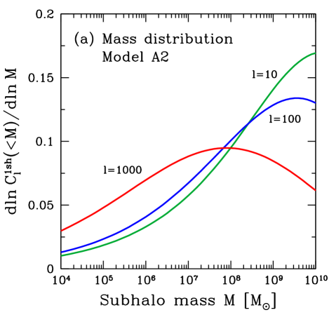
In fact, we can understand this qualitatively, by analyzing the integrand of Eq. (19). In Fig. 8, we show contributions to from unit logarithmic mass range and from unit logarithmic distance () range. The mass distributions [Fig. 8(a)] peak at high-mass range close to , but are broader for smaller angular scales. This is because at small angular scales, massive subhalos are regarded as extended, suppressing the power; note that is a decreasing function of for fixed . Subhalo masses averaged over this distribution and corresponding scale radii are and kpc (), and kpc (), and and kpc (). Now, Fig. 8(b) shows that the contribution from farther subhalos is more important for smaller angular scales, since the closer subhalos are more extended. Features at 15 kpc correspond to , below which contribution from massive subhalos are not included as they are identified as individual sources. Distances averaged over this distribution are kpc (), 20 kpc (), and 32 kpc (). Combining these typical distance scales with the scale radii, we find that the angular extension of the subhalos is typically 6.6∘ (), 3.9∘ (), and 1.9∘ (). For the latter two scales, the subhalo extensions are larger than the angular scales probed () and thus typical subhalos are extended, but for the case of , they are almost point-like sources. Therefore, as we see in Fig. 7(a), the one-subhalo term starts to deviate from the white noise above .
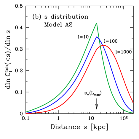
In Figs. 9(a) and 10, we show the angular power spectrum, and mass and radius distributions, respectively, for the other fiducial model A2 (). The amplitude of the angular power spectrum for the one-subhalo term is much larger than that for the model A1, whereas the spectrum shape is almost unchanged. This dependence and its interpretation are the same as those discussed in Sec. III.2 for simplified subhalo models (see Figs. 3 and 4). The mass and distance distributions for are almost the same as the case of the model A1.
We now discuss the detectability of the angular power spectrum. The one-sigma errors of can be estimated as
| (27) |
where is the bin width for that we take , and is the Gaussian window function with the beam size of the Fermi (for 10-GeV photons). The noise power spectrum is associated with the finite photon count and it is related to number of signal () and background photons () through . For we assume that half of the EGRET gamma-ray background intensity remains unresolved with Fermi, thus , where cm-2 s-1 sr-1, cm2 is effective area, s is effective exposure time, for which we assume 5-yr all-sky survey ( yr and sr is the field of view of Fermi). The background due to detector noise is negligible for Fermi, and at high latitudes, the galactic foreground due to cosmic-ray propagation will be relatively small compared with the isotropic component of the gamma-ray background Strong2004 (but see also Ref. Keshet2004 ). Hence we approximate and obtain sr.
We here consider a multiple-component scenario in which the observed total gamma-ray intensity comes mainly from several origins. We assume these are dark matter subhalos, smooth dark matter component in the host, and an astrophysical source such as blazars:
| (28) |
and we define each fraction by
| (29) |
where for simplicity, we represent the angle and ensemble-averaged intensity by , and the subscript “b” stands for blazars. Then, the total angular power spectrum corresponding to the total intensity is given by
| (30) |
As galactic dark matter and blazars (or any other extragalactic sources) are independently distributed in space, cross-correlation terms, and can be safely neglected. The other cross term will be nonzero, but the amplitude of should be at most comparable to or . Therefore, we shall neglect all the cross-correlation terms in the following discussions; this is conservative because adding this additional component would work favorably for dark matter detection. is the subhalo angular power spectrum and is the same as Eq. (18) that we closely investigated thus far. The host-halo intensity is given by
| (31) |
and for the models A1 and A2, we have and 0.16, respectively. Therefore, the host-halo component would be small in the mean intensity, and therefore would be further suppressed in the angular power spectrum. To estimate the blazar power spectrum , we use the luminosity dependent density evolution model for the gamma-ray luminosity function Narumoto2006 ; Ando2007b , and approximate as nearly a Poisson noise, sr, which is good especially for Ando2007a . We should use the in the right-hand side of Eq. (27) to estimate the errors for subhalo signal . Here we are not interested in the blazars and treat them as a reducible component by using lower-energy data; see Ref. Ando2007a for a more detailed discussion.
In the following analysis, we take as a free parameter instead of others such as and . We neglect the host-halo term as it is always smaller than the subhalo term, and so . In Fig. 7(b), we show errors of the angular power spectrum, , for the model A1, when and . This shows that if subhalos give a fractional contribution to the mean background intensity, it could also be detected in the angular power spectrum, especially at . Figure 9(b) is the same but for the model A2 and and . In this case, the detection is more promising as the subhalo anisotropy is much larger than that of blazars, and signal-to-noise ratio exceeds 1 for a wide multipole range, reaching maximum at . Therefore, we define detection criterion by setting at either or 100, where is the signal-to-noise ratio, and for the fiducial models, the value of required to satisfy this criterion is (A1) and 0.038 (A2). (Although it is for only one-sigma detection, we could also use other multipole bins to increase significance.) For the model A1, in order to achieve , we need additional boost of . For this boost factor, the expected number of subhalo detection is . We also find that associated gamma-ray flux from the galactic center still satisfies constraint from EGRET Mayer-Hasselwander1998 , i.e., , even if the cusp of the NFW profile extends to the very center. Thus, the angular power spectrum could be a stronger probe than detection as single identified sources. For the model A2, the values for these quantities associated with the anisotropy detection are , , and . As this model features smaller mean intensity, we need relatively large boost to give a small fraction (4%) for anisotropy detection. Accordingly, the associated number of subhalo detection is a few, but it is still not very many. Furthermore, the number of subhalo detection potentially fluctuates to give . Even in this case, the anisotropy analysis, therefore, might provide equally sensitive, but statistically more stable method to probe dark matter annihilation in the galactic substructure. The spectra of the mean intensity for these models A1 and A2 with the boost of are shown in Fig. 6.
IV.3 Dependence on models and parameters
| Model | ||||||||||||
| A1 (fiducial) | 1.9 | 0.2 | 2 | 0.0064 | 0.24 | 13 | 0.64 | 0.028 | ||||
| A2 (fiducial) | 1.9 | 0.16 | 2 | 0.16 | 0.038 | 53 | 4.0 | 0.12 | ||||
| B1 | 1.9 | 0.2 | 2 | 0.21 | 1.4 | 0.72 | 0.010 | |||||
| B2 | 1.9 | 0.16 | 2 | 0.021 | 0.069 | 13 | 12 | 0.033 | ||||
| C1a | 2.0 | 0.5 | 5 | 0.24 | 0.37 | 0.016 | 0.0014 | |||||
| C1b | 1.8 | 0.15 | 2 | 0.068 | 0.090 | 47 | 3.2 | 0.11 | ||||
| D2 | 1.9 | 0.16 | 2 | 0.16 | 0.11 | 170 | 17 | 0.39 |
In this subsection, we investigate dependence of results on models and parameters for subhalos. In Table 1, we show models with that we investigate the dependence on , subhalo distribution (unbiased versus anti-biased), presence of sub-substructure, as listed in the second to seventh columns of the table (we fix ). The first two models are the fiducial models, on which we focused in the previous subsection. The next two “B” models are for the unbiased subhalo distribution. Models C1a and C1b is the same as A1 but for different mass function. Lastly, the model D2 is the same as A2 but the subhalos feature much more extended emissivity profile, proportional to the density , which might be the case if there are a lot of sub-substructure remaining in the subhalos.
In Fig. 11, we show angular power spectrum (one-subhalo term ) of B1 and B2 (unbiased), compared with A1 and A2 (anti-biased). For all the models investigated, the angular power spectrum is larger for the anti-biased distribution than the unbiased one. This tendency is the same as we have seen in the previous section for point-like subhalos. Furthermore, deviation from the white noise at small angular scales is slightly more significant for the unbiased distribution. This is because the relevant subhalos are closer in the case of the unbiased model (see Fig. 1), and therefore, they are more extended.
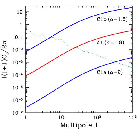
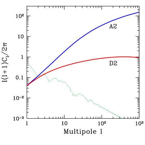
In Fig. 12, we compare the models C1a and C1b with the fiducial model A1, to study dependence on . The shape of the power spectrum is almost the same among these models and the amplitudes follow the same tendency as seen in Fig. 4. Figure 13 shows a more extended model D2 where we assume that the gamma-ray luminosity is proportional to the density . The suppression of the power spectrum at small angular scales is even more prominent for the more extended emissivity profile, which makes it more difficult for this model to be detected with anisotropy signals.
Table 1 also shows results of host-to-subhalo ratio for the mean intensity, . In any of these models, the host-halo component is always smaller than the subhalo component in the mean intensity. It is, therefore, even more suppressed in the angular power spectrum. We also show values of and the particle-physics parameter (in units of ) necessary to boost the subhalo signals to the level of where is either 10 or 100. For any of these models, we find that if the subhalo contribution is as high as 20%, it should be detected in the angular power spectrum, a similar conclusion as obtained for the extragalactic dark matter signal Ando2007a . For the models that feature large such as A2, B2, and C1b, the sensitivity of Fermi for could reach down to several to ten percent level. We note that to boost the anisotropy signal to the detectable level, we only need modest values for the particle physics parameter, –100. The quantities and associated with anisotropy detection are summarized in the last two columns of Table 1. The former ranges from less than one to 10. All the models satisfy a constraint from the gamma-ray flux from the galactic center.
V Discussion
Our results confirm what was found in the previous papers Siegal-Gaskins2008 ; Fornasa2009 ; i.e., the angular power spectrum is dominated by the noise-like term with a stronger suppression at higher multipoles. In particular, behaviors of for the models where subhalos luminosity profile is proportional to its density squared, are very similar to the power spectrum obtained in Refs. Siegal-Gaskins2008 ; Fornasa2009 . This is quite natural because these authors also assumed similar profiles. Our formulation, not only gives physical explanations of these results, but also enables to investigate other cases such that the luminosity profile is simply proportional to density, where the suppression at small scales is even more pronounced.
For the flux sensitivity of Fermi, we adopted cm-2 s-1 for GeV, but this is only for sources whose extension is smaller than the beam size (point-like sources). If the sources are extended as is the case for massive subhalos, then the flux sensitivity is worse, and thus becomes smaller. This will decrease expected number of subhalo detection, , because it considerably reduces effective volume. Thus the conclusions given in the previous section might be rather conservative, and the anisotropy analysis could be even better, compared with the detection of subhalos as identified sources.
Throughout our calculations, we took into account the effect of tidal destruction of subhalos by using the anti-biased distribution, since stronger gravitational potential around a central region of the host halo is expected to work more efficiently to get rid of more subhalos. We also took into account the fact that the subhalos feature higher concentration than field halos of the same mass. This might be more complicated because the tidal force is more effective towards the galactic center, and therefore, the subhalos are more concentrated there. This is indeed confirmed by recent numerical simulations, where concentration parameters scale as a function of galactocentric radius as Diemand2008 . Although this effect was not taken into account in our calculations, we could do that quite easily by using our analytic formulae with slight modification.
We did not consider dark matter annihilation in the extragalactic halos in this study, which should also contribute to the isotropic gamma-ray background. We note, however, that this component might be comparable to that from the galactic subhalos Oda2005 ; Fornasa2009 , being smaller by only a factor of a few. The anisotropy structure for this component has been investigated in Refs. Ando2006 ; Ando2007a , and found that the angular power spectrum could also be reasonably large, for Ando2007a . Including this component further complicates the analysis, but should be performed when the actual Fermi data became accessible.
Although we focused on gamma-ray photons with GeV, analysis of angular power spectrum can be performed at any photon energies. In principle, one could use an energy spectrum of the angular fluctuation as another diagnosis Ando2006 ; Siegal-Gaskins2009 , although we do not discuss it further.
VI Conclusions
To conclude, we investigated the angular power spectrum of the gamma-ray background from dark matter annihilation in galactic substructure. Our main findings are the followings.
-
1.
In contrast to the earlier works Siegal-Gaskins2008 ; Fornasa2009 that relied mainly on mock gamma-ray maps generated numerically, we derived analytic formulae that enable to compute the angular power spectrum directly with assumed subhalo models (Sec. II). The angular power spectrum consists of two terms: one-subhalo and two-subhalo terms [Eq. (18)].
-
2.
The two-subhalo term [Eq. (20)] depends on smooth (ensemble averaged) distribution function of subhalos within the parent halo, . This is largely independent of internal density structure of the subhalos. We evaluated this term using the HEALPix numerical package Gorski2005 and show that the contribution is considerably small at small angular scales (e.g., Fig. 3).
-
3.
The one-subhalo term [Eq. (19)] depends on luminosity profile of each subhalo as well as number of subhalos that give significant contribution to the mean intensity of the gamma-ray background. When the subhalo extension can be neglected (point-like sources), it simply is the Poisson noise [Eq. (23)]. In this case, if the subhalo mass function is close to as implied by recent numerical simulations, depends on the lower mass cutoff as well as whether the subhalos follow the unbiased or anti-biased distribution in the parent halo (Fig. 4).
-
4.
Taking into account radial extension of the subhalos emissivity profile suppresses the power spectrum at small angular scales, through (Fourier transform of the emissivity profile) of Eq. (19). As fiducial subhalo models, we assume that the emissivity profile follows internal density squared, as well as the mass spectrum, and the anti-biased subhalo distribution within the host. We adopt and as a minimum mass of the subhalos. The angular power spectrum is suppressed compared with the white noise at angular scales smaller than 10∘ because of the extended intensity profile (Figs. 7 and 9). If , the angular scales around 10∘ is favored for detection, where the power spectrum is dominated by the two-subhalo term. For the anisotropy detection, the required fractional contribution to the mean intensity is 20%, for which we need additional boost of 10. The associated number of subhalo detection as individual sources is less than one. If , on the other hand, the amplitude of the angular power spectrum (one-subhalo term) is much larger than the former case, and therefore, smaller angular scales 1∘ would be more promising for detection. The fractional intensity necessary for anisotropy detection could be as small as 4%, for which the boost is 50 and the associated number of subhalo detection is 4. Therefore, the analysis of the angular power spectrum might be stronger than the detection of subhalos as identified gamma-ray sources, and furthermore, could provide more statistically stable approach to the same problem.
-
5.
We also investigated dependence on subhalo parameters by considering several models (including the fiducial ones) summarized in Table 1. We found that the amplitude of the angular power spectrum is smaller for the unbiased model compared with the anti-biased model (Fig. 11), and for a softer mass function (Fig. 12). The angular power spectrum for models featuring more extended luminosity profile due to dominance by sub-subhalo component is significantly suppressed at small scales (Figs. 13) and is more difficult to detect with Fermi.
Acknowledgements.
The author is grateful to Eiichiro Komatsu for valuable discussions, and thanks Gianfranco Bertone, Samuel Lee, and Jennifer Siegal-Gaskins for comments. This work was supported by the Sherman Fairchild Foundation.Appendix A Number density of subhalos
Here we obtain number density of subhalos by relating it to the mass of the Milky-Way halo, for both the unbiased and anti-biased models. It is obtained by requiring
| (32) |
and using Eq. (21). It is also useful to note the following relation:
| (33) |
where is the concentration parameter for the Milky-Way halo.
We thus obtain, for the unbiased case,
| (34) |
For the anti-biased case, we assume that the subhalo distribution follows Einasto profile Einasto1969 , , where is a scale radius at which the density slope is . With a proper normalization, we obtain
| (37) | |||||
where is the lower incomplete gamma function, and . For numerical values of the parameters, we adopt and Springel2008a .
Appendix B Fourier transform of emissivity profile
The emissivity profile somehow follows density profile of subhalos. If it is smooth, then , whereas if they include a number of sub-subhalos, then it scales more like . Here we compute the Fourier transform of this quantity, . When the density profile of the subhalos are well described by the NFW profile up to a cutoff radius , then the both cases have analytic expressions for given concentration and scale radius. These forms are somewhat complicated, and thus we instead give fitting formulae that give excellent approximation for a wide range of reasonable values of . For the both cases, the fitting form is
| (38) |
For (no sub-subhalos), , , and , and these values are largely independent of . On the other hand, for (with sub-subhalos), we have , , and .
References
- (1) G. Jungman, M. Kamionkowski and K. Griest, Phys. Rep. 267, 195 (1996) [arXiv:hep-ph/9506380].
- (2) D. Hooper and S. Profumo, Phys. Rep. 453, 29 (2007) [arXiv:hep-ph/0701197].
- (3) G. Bertone, D. Hooper and J. Silk, Phys. Rep. 405, 279 (2005) [arXiv:hep-ph/0404175].
- (4) F. W. B. Atwood [LAT Collaboration], Astrophys. J. 697, 1071 (2009) [arXiv:0902.1089 [astro-ph.IM]].
- (5) E. A. Baltz et al., JCAP 0807, 013 (2008) [arXiv:0806.2911 [astro-ph]].
- (6) B. Moore, S. Ghigna, F. Governato, G. Lake, T. Quinn, J. Stadel and P. Tozzi, Astrophys. J. 524, L19 (1999).
- (7) A. A. Klypin, A. V. Kravtsov, O. Valenzuela and F. Prada, Astrophys. J. 522, 82 (1999) [arXiv:astro-ph/9901240].
- (8) J. Diemand, B. Moore, and J. Stadel, Nature 433, 389 (2005) [arXiv:astro-ph/0501589].
- (9) J. Diemand, M. Kuhlen and P. Madau, Astrophys. J. 649, 1 (2006) [arXiv:astro-ph/0603250].
- (10) S. Hofmann, D. J. Schwarz and H. Stoecker, Phys. Rev. D 64, 083507 (2001) [arXiv:astro-ph/0104173].
- (11) A. M. Green, S. Hofmann and D. J. Schwarz, JCAP 0508, 003 (2005) [arXiv:astro-ph/0503387].
- (12) A. Loeb and M. Zaldarriaga, Phys. Rev. D 71, 103520 (2005) [arXiv:astro-ph/0504112].
- (13) S. Profumo, K. Sigurdson and M. Kamionkowski, Phys. Rev. Lett. 97, 031301 (2006) [arXiv:astro-ph/0603373].
- (14) E. Bertschinger, Phys. Rev. D 74, 063509 (2006) [arXiv:astro-ph/0607319].
- (15) V. Berezinsky, A. Bottino and G. Mignola, Phys. Lett. B 325, 136 (1994) [arXiv:hep-ph/9402215].
- (16) L. Bergstrom, P. Ullio and J. H. Buckley, Astropart. Phys. 9, 137 (1998) [arXiv:astro-ph/9712318].
- (17) A. Cesarini, F. Fucito, A. Lionetto, A. Morselli and P. Ullio, Astropart. Phys. 21, 267 (2004) [arXiv:astro-ph/0305075].
- (18) N. Fornengo, L. Pieri and S. Scopel, Phys. Rev. D 70, 103529 (2004) [arXiv:hep-ph/0407342].
- (19) S. Dodelson, D. Hooper and P. D. Serpico, Phys. Rev. D 77, 063512 (2008) [arXiv:0711.4621 [astro-ph]].
- (20) L. Bergstrom, J. Edsjo, P. Gondolo and P. Ullio, Phys. Rev. D 59, 043506 (1999) [arXiv:astro-ph/9806072].
- (21) C. Calcaneo-Roldan and B. Moore, Phys. Rev. D 62, 123005 (2000) [arXiv:astro-ph/0010056].
- (22) A. Tasitsiomi and A. V. Olinto, Phys. Rev. D 66, 083006 (2002) [arXiv:astro-ph/0206040].
- (23) F. Stoehr, S. D. M. White, V. Springel, G. Tormen and N. Yoshida, Mon. Not. R. Astron. Soc. 345, 1313 (2003) [arXiv:astro-ph/0307026].
- (24) N. W. Evans, F. Ferrer and S. Sarkar, Phys. Rev. D 69, 123501 (2004) [arXiv:astro-ph/0311145].
- (25) R. Aloisio, P. Blasi and A. V. Olinto, Astrophys. J. 601, 47 (2004) [arXiv:astro-ph/0206036].
- (26) S. M. Koushiappas, A. R. Zentner and T. P. Walker, Phys. Rev. D 69, 043501 (2004) [arXiv:astro-ph/0309464].
- (27) J. Diemand, M. Kuhlen and P. Madau, Astrophys. J. 657, 262 (2007) [arXiv:astro-ph/0611370].
- (28) L. Pieri, G. Bertone and E. Branchini, Mon. Not. R. Astron. Soc. 384, 1627 (2008) [arXiv:0706.2101 [astro-ph]].
- (29) L. E. Strigari, S. M. Koushiappas, J. S. Bullock, M. Kaplinghat, J. D. Simon, M. Geha and B. Willman, Astrophys. J. 678, 614 (2008) [arXiv:0709.1510 [astro-ph]].
- (30) M. Kuhlen, J. Diemand and P. Madau, Astrophys. J. 686, 262 (2008) [arXiv:0805.4416 [astro-ph]].
- (31) G. D. Martinez, J. S. Bullock, M. Kaplinghat, L. E. Strigari and R. Trotta, arXiv:0902.4715 [astro-ph.HE].
- (32) S. M. Koushiappas, Phys. Rev. Lett. 97, 191301 (2006) [arXiv:astro-ph/0606208].
- (33) S. Ando, M. Kamionkowski, S. K. Lee and S. M. Koushiappas, Phys. Rev. D 78, 101301(R) (2008) [arXiv:0809.0886 [astro-ph]].
- (34) L. Bergstrom, J. Edsjo and P. Ullio, Phys. Rev. Lett. 87, 251301 (2001) [arXiv:astro-ph/0105048].
- (35) P. Ullio, L. Bergstrom, J. Edsjo and C. G. Lacey, Phys. Rev. D 66, 123502 (2002) [arXiv:astro-ph/0207125].
- (36) J. E. Taylor and J. Silk, Mon. Not. R. Astron. Soc. 339, 505 (2003) [arXiv:astro-ph/0207299].
- (37) D. Elsaesser and K. Mannheim, Phys. Rev. Lett. 94, 171302 (2005) [arXiv:astro-ph/0405235].
- (38) S. Ando, Phys. Rev. Lett. 94, 171303 (2005) [arXiv:astro-ph/0503006].
- (39) T. Oda, T. Totani and M. Nagashima, Astrophys. J. 633, L65 (2005) [arXiv:astro-ph/0504096].
- (40) S. Horiuchi and S. Ando, Phys. Rev. D 74, 103504 (2006) [arXiv:astro-ph/0607042].
- (41) S. Ando and E. Komatsu, Phys. Rev. D 73, 023521 (2006) [arXiv:astro-ph/0512217].
- (42) S. Ando, E. Komatsu, T. Narumoto and T. Totani, Phys. Rev. D 75, 063519 (2007) [arXiv:astro-ph/0612467].
- (43) A. Cuoco, S. Hannestad, T. Haugbolle, G. Miele, P. D. Serpico and H. Tu, JCAP 0704, 013 (2007) [arXiv:astro-ph/0612559].
- (44) A. Cuoco, J. Brandbyge, S. Hannestad, T. Haugboelle and G. Miele, Phys. Rev. D 77, 123518 (2008) [arXiv:0710.4136 [astro-ph]].
- (45) L. Zhang and G. Sigl, JCAP 0809, 027 (2008) [arXiv:0807.3429 [astro-ph]].
- (46) M. Taoso, S. Ando, G. Bertone and S. Profumo, Phys. Rev. D 79, 043521 (2009) [arXiv:0811.4493 [astro-ph]].
- (47) J. M. Siegal-Gaskins, JCAP 0810, 040 (2008) [arXiv:0807.1328 [astro-ph]].
- (48) M. Fornasa, L. Pieri, G. Bertone and E. Branchini, arXiv:0901.2921 [astro-ph].
- (49) D. Hooper and P. D. Serpico, JCAP 0706, 013 (2007) [arXiv:astro-ph/0702328].
- (50) H. Yuksel, S. Horiuchi, J. F. Beacom and S. Ando, Phys. Rev. D 76, 123506 (2007) [arXiv:0707.0196 [astro-ph]].
- (51) S. K. Lee, S. Ando and M. Kamionkowski, arXiv:0810.1284 [astro-ph].
- (52) S. Dodelson, A. V. Belikov, D. Hooper and P. Serpico, arXiv:0903.2829 [astro-ph.CO].
- (53) J. F. Navarro, C. S. Frenk and S. D. M. White, Astrophys. J. 490, 493 (1997) [arXiv:astro-ph/9611107].
- (54) A. Klypin, H. Zhao and R. S. Somerville, Astrophys. J. 573, 597 (2002) [arXiv:astro-ph/0110390].
- (55) S. Ghigna, B. Moore, F. Governato, G. Lake, T. R. Quinn and J. Stadel, Astrophys. J. 544, 616 (2000) [arXiv:astro-ph/9910166].
- (56) G. De Lucia et al., Mon. Not. Roy. Astron. Soc. 348, 333 (2004) [arXiv:astro-ph/0306205].
- (57) L. Gao, S. D. M. White, A. Jenkins, F. Stoehr and V. Springel, Mon. Not. Roy. Astron. Soc. 355 (2004) 819 [arXiv:astro-ph/0404589].
- (58) L. Shaw, J. Weller and J. P. Ostriker, Astrophys. J. 659, 1082 (2007) [arXiv:astro-ph/0603150].
- (59) J. Diemand, M. Kuhlen and P. Madau, Astrophys. J. 667, 859 (2007) [arXiv:astro-ph/0703337].
- (60) U. Seljak, Mon. Not. R. Astron. Soc. 318, 203 (2000) [arXiv:astro-ph/0001493].
- (61) A. V. Kravtsov, A. A. Berlind, R. H. Wechsler, A. A. Klypin, S. Gottloeber, B. Allgood and J. R. Primack, Astrophys. J. 609, 35 (2004) [arXiv:astro-ph/0308519].
- (62) A. R. Zentner, A. A. Berlind, J. S. Bullock, A. V. Kravtsov and R. H. Wechsler, Astrophys. J. 624, 505 (2005) [arXiv:astro-ph/0411586].
- (63) P. J. E. Peebles, The Large-Scale Structure of the Universe (Princeton University Press, Princeton, NJ, 1980).
- (64) J. Einasto, Tr. Inst. Astrofiz. Alma-Ata 5, 87.
- (65) V. Springel et al., Mon. Not. R. Astron. Soc. 391, 1685 (2008) [arXiv:0809.0898 [astro-ph]].
- (66) D. Nagai and A. V. Kravtsov, Astrophys. J. 618, 557 (2005) [arXiv:astro-ph/0408273].
- (67) A. R. Wetzel, J. D. Cohn and M. White, arXiv:0810.3650 [astro-ph].
- (68) P. Sreekumar et al. [EGRET Collaboration], Astrophys. J. 494, 523 (1998) [arXiv:astro-ph/9709257].
- (69) K. M. Gorski, E. Hivon, A. J. Banday, B. D. Wandelt, F. K. Hansen, M. Reinecke and M. Bartelman, Astrophys. J. 622, 759 (2005) [arXiv:astro-ph/0409513].
- (70) S. Kazantzidis, L. Mayer, C. Mastropietro, J. Diemand, J. Stadel and B. Moore, Astrophys. J. 608, 663 (2004) [arXiv:astro-ph/0312194].
- (71) F. Stoehr, S. D. M. White, G. Tormen and V. Springel, Mon. Not. R. Astron. Soc. 335, L84 (2002) [arXiv:astro-ph/0203342].
- (72) E. Hayashi, J. F. Navarro, J. E. Taylor, J. Stadel and T. R. Quinn, Astrophys. J. 584, 541 (2003) [arXiv:astro-ph/0203004].
- (73) J. Penarrubia, A. McConnachie and J. F. Navarro, Astrophys. J. 672, 904 (2008) [arXiv:astro-ph/0701780].
- (74) V. Springel et al., Nature 456, 73 (2008) [arXiv:0809.0894 [astro-ph]].
- (75) J. S. Bullock et al., Mon. Not. R. Astron. Soc. 321, 559 (2001) [arXiv:astro-ph/9908159].
- (76) M. Kuhlen, L. E. Strigari, A. R. Zentner, J. S. Bullock and J. R. Primack, Mon. Not. R. Astron. Soc. 357, 387 (2005) [arXiv:astro-ph/0402210].
- (77) A. V. Macciò, A. A. Dutton, F. C. van den Bosch, B. Moore, D. Potter and J. Stadel, Mon. Not. R. Astron. Soc. 378, 55 (2007) [arXiv:astro-ph/0608157].
- (78) A. F. Neto et al., Mon. Not. R. Astron. Soc. 381, 1450 (2007) [arXiv:0706.2919 [astro-ph]].
- (79) A. W. Strong, I. V. Moskalenko and O. Reimer, Astrophys. J. 613, 962 (2004) [arXiv:astro-ph/0406254].
- (80) U. Keshet, E. Waxman and A. Loeb, JCAP 0404, 006 (2004) [arXiv:astro-ph/0306442].
- (81) T. Narumoto and T. Totani, Astrophys. J. 643, 81 (2006) [arXiv:astro-ph/0602178].
- (82) S. Ando, E. Komatsu, T. Narumoto and T. Totani, Mon. Not. R. Astron. Soc. 376, 1635 (2007) [arXiv:astro-ph/0610155].
- (83) H. A. Mayer-Hasselwander et al., Astron. Astrophys. 335, 161 (1998).
- (84) J. Diemand, M. Kuhlen, P. Madau, M. Zemp, B. Moore, D. Potter and J. Stadel, Nature 454, 735 (2008) [arXiv:0805.1244 [astro-ph]].
- (85) J. M. Siegal-Gaskins and V. Pavlidou, arXiv:0901.3776 [astro-ph.HE].