Existence, uniqueness and convergence of a particle approximation for the Adaptive Biasing Force process
Abstract
We study a free energy computation procedure, introduced in [5, 8], which relies on the long-time behavior of a nonlinear stochastic differential equation. This nonlinearity comes from a conditional expectation computed with respect to one coordinate of the solution. The long-time convergence of the solutions to this equation has been proved in [11], under some existence and regularity assumptions.
In this paper, we prove existence and uniqueness under suitable conditions for the nonlinear equation, and we study a particle approximation technique based on a Nadaraya-Watson estimator of the conditional expectation. The particle system converges to the solution of the nonlinear equation if the number of particles goes to infinity and then the kernel used in the Nadaraya-Watson approximation tends to a Dirac mass.
We derive a rate for this convergence, and illustrate it by numerical examples on a toy model.
1 Université Paris-Est, CERMICS, 6 et 8 avenue Blaise Pascal, 77455 Marne-La-Vallée Cedex 2, France
2 Université Paris-Est, CERMICS, Project-Team MICMAC ENPC-INRIA, 6 et 8 avenue Blaise Pascal, 77455 Marne-La-Vallée Cedex 2, France
Introduction
Free energy computations are an important problem in the field of molecular simulation (see [4]). The difficulty of those computations lies in the fact that most dynamics in molecular simulations are highly metastable: many free energy barriers prevent a good sampling. We study here the adaptive biasing force (ABF) method, which was introduced in [5, 8] to get rid of those metastabilities.
The typical problems one can think about are the study of a structural angle in the conformation of a protein, or the measure of the evolution of a chemical reaction. Mathematically, each configuration of the system is modelized by an element of a high-dimensional state space , typically an open subset of , which is endowed with a probability measure, called the canonical measure. This measure is given by , where denotes the potential energy undergone by the physical system, and is proportional to the inverse of the temperature of the system.
For some in the state space, one is interested in a particular quantity, denoted by , being
assumed to be a smooth function from to the one-dimensional
torus . The quantity has to be understood as a coarse-grained
information on the system, which is the relevant information for the
practitioner. In the examples above, would be a structural
angle in a protein with conformation ,
or a number measuring the evolution of a chemical system in state .
We call free energy the effective energy associated to the
quantity
, that is, the function such that
is the image measure of the canonical measure by the function .
Our objective is to compute numerically the function .
When , a naive method to do so is to simulate, for a given random variable
and an independent valued Brownian motion , the process defined by the
(overdamped) Langevin dynamics
| (0.1) |
which, under some regularity assumptions on the potential, is ergodic and admits the canonical measure as unique invariant measure. This approach appears to be untractable in practice, since the convergence to equilibrium is very slow, due to multiple metastabilities appearing in most problems: typically, a molecule moves microscopically within times of order seconds, while the typical time scale of the macroscopic moves is of order seconds.
The idea of the ABF method is to prevent the process from staying in metastable states by introducing a biasing force which repel from the states where it stayed for too long a time. To do this, we use the following representation of , that can be deduced from the co-area formula (see [11]):
| (0.2) |
where is a random variable distributed according to the canonical measure, and is the function defined by
| (0.3) |
The function is called the mean force. Actually, (0.2) also holds when is distributed according to the measure
which is the canonical measure associated with the biased potential where is any smooth function.
Equation (0.2) leads us to consider the following dynamics, which should get rid of metastabilities for a well chosen since it “flattens” the energy landscape in the direction (see [11] and Lemma 1.2 below for more precise statements):
| (0.4) |
The second equality in (0.4) shows that if is distributed according to the canonical measure associated with the potential , then the biasing force is actually the derivative of the free energy, and the first equation in (0.4) consists in a Langevin dynamics associated to the potential . Consequently, the dynamics (0.4) admits a stationary point: and .
If we actually have convergence to this stationary state, we have a method, that should be efficient (i.e. that should not see the metastabilities), to sample the canonical measure up to a known perturbation This algorithm has thus two applications: it allows the computation of the free energy , and it can be used as an adaptative importance sampling method for the canonical measure.
The long time behavior of Equation (0.4) has been studied in [11], where it has been proven that for a sufficiently regular solution, one has, in some sense, an exponential convergence to the stationary state, with a rate that is better (for a well chosen ) than the rate of convergence to equilibrium for (0.1).
The practical difficulty in simulating (0.4) is to compute the conditional expectation, which is a highly nonlinear term. Stochastic differential equations involving conditional expectations have already been studied, in a case where the conditional expectation is computed with respect to a random initial condition (see [16, 18]) or where the variable whose conditional expectation is computed is fixed (see [7]). Our situation is much more complex since both the conditioning and the conditioned variables change with time and are affected by the previous conditional expectations.
The same difficulty arises in Lagrangian stochastic models which are commonly used in the simulation of turbulent flows (see [2]). The main difference between the system studied in [2] and (0.4) is that the authors considers a Langevin dynamics with noise only on the velocity. The lack of ellipticity then leads to additional difficulties. In our setting we are able to derive a quantitative error estimate for the particle discretization while this seems more difficult for Langevin dynamics.
In this paper, we prove that existence and uniqueness hold for Equation (0.4) under suitable conditions, and we study an approximation of by an interacting particle system (see Theorems 1.3 and 1.4 below).
The paper is organized as follows. In Section 1 we state our main results.
Section 2 is devoted to some uniqueness and regularity results. More precisely, we prove that the time marginals of a solution to Equation (0.4) satisfy some partial differential equation. Then, under an integrability condition on the initial condition, we prove uniqueness for the solutions to this equation, so that the nonlinear term in (0.4) is reduced to a bounded drift coefficient. We thus prove pathwise uniqueness and uniqueness in distribution for the solutions of (0.4).
Section 3 is devoted to existence results. More precisely, we introduce a regularization of the dynamics (0.4) involving two parameters and , which is another nonlinear stochastic differential equation whose nonlinearity is less singular. We prove that strong existence, pathwise uniqueness and uniqueness in distribution hold for this equation and then we show that the solutions to this stochastic differential equation converge to some process which satisfies (0.4) in the limit , yielding strong existence. We also prove that this convergence holds with rate .
In Section 4 we introduce an interacting particle system to approximate the regularized dynamics, and we prove a propagation-of-chaos result for this particle system. We also derive a rate of convergence for this propagation of chaos.
In Section 5, we illustrate the efficiency of the particle approximation of the ABF method and the rate of those convergences with some numerical examples in small dimension.
Acknowledgement : We warmly thank Mathias Rousset for his careful reading of an early version of the manuscript.
Notation
We denote by the one dimensional torus, and for , we denote by its projection on . In the following, we will work in two different domains : or . The case will be called the non compact case, and the case will be called the compact case. For , depending on the case considered, we will also denote by the element of (resp. ) defined by (resp. ).
In the following, we will call “function defined on ” (resp. on , resp. on ), a periodical (resp. periodical in the first coordinate, resp. -periodical) function defined on (resp on ). Integrals on , or mean integrals on , or .
We denote by the space of functions on whose square is integrable on , and by the space of functions in whose weak gradient is square integrable on . We use similar notations on and
For two functions and defined on or , we denote the convolution with respect to the first coordinate, that is,
If is defined on , we also use the notation to denote
When and are defined on or , the convolution in all the coordinates is denoted :
In the following, we call “probability measure on ” (resp. on , ) a nonnegative -periodical (resp. -periodical with respect to the first coordinate, -periodical) measure such that (resp , ).
When is a random variable taking values in (resp. in , ), we call “distribution of ” or “law of ” the probability measure on (resp. on , ) such that
For a given probability measure on (resp. a probability density ) and a given bounded function , we denote (resp. ) the marginal on of the measure (resp. ). Namely:
and
In particular, is the first coordinate marginal of . When we do not specify the measure in an integral, it is the Lebesgue measure.
We will need the weighted spaces
for , and
with , for some Notice that does not depend on the first coordinate , and that there is a positive constant such that
| (0.5) |
We will use several times the following statement:
Lemma 0.1.
For a bounded function , and one has, for some constant ,
If moreover, has bounded derivatives and , then
The same inequalities hold with the non weighted norms in the right-hand side, for respectively in and .
Proof.
Recall that we assumed , so that is integrable on : . Consequently, we have the estimation
The proof is similar in the space . ∎
In the following, will denote some positive constant, whose value can change from line to line.
1 Assumptions and statement of the main results
In this paper, we consider a particular case of Equation (0.4) to simplify the argumentation: we assume (this can be realized by a change of variable), or . We consider as reaction coordinate the first coordinate function defined by This should not change the theoretical results, but will simplify the proofs. The definition (0.3) of is then reduced to
where is defined on or
The two settings and will be respectively called the compact and the non-compact case. Our results hold in both settings, and the proofs are mostly identical, with some slight additional difficulties in the non compact case. Thus, in those situations, we only give the proofs in the non-compact case.
With those assumptions, Equation (0.4) rewrites
| (1.1) |
denoting the first vector in the canonical basis of . We will call solution to Equation (1.1) a process where satisfies (1.1). The initial condition of (1.1) is a random variable denoted , and is supposed to be independent of the Brownian motion . We denote by the law of which is a probability measure on
To ensure the integrability of , we make the following assumption :
Assumption i.
is a twice continuously differentiable function, which has bounded first and second order partial derivatives.
Notice that Assumption i yields boundedness of the drift coefficient in (1.1). In the compact case, assumption i is satisfied as soon as is a twice differentiable function.
We have to make some assumptions on the initial condition . What is needed to prove our results will depend on whether we consider the compact or the non compact case. In the compact case, we consider the following assumption:
Assumption ii.
The probability measure has a density lying in and whose first coordinate marginal is bounded from below by a positive constant. (Notice that is a probability density on .)
In the non compact case, we will need a stronger assumption: we have to control the decay of the initial condition at infinity, so we work in the weighted space . We will use, in addition to Assumption ii, the following one:
Assumption iii.
The density of lies in both and .
Notice that Assumptions iii implies that has finite moments of order less than , and that Assumption i then yields a control on the corresponding moments of any solution to (1.1), uniformly in :
Lemma 1.1.
Proof.
This comes from the boundedness of the drift coeficient , which holds in regard of Assumption i. Indeed, we have , which is bounded on . ∎
According to the following fundamental lemma, the solution to (1.1) is going to sample efficiently the coordinate reaction state space
Lemma 1.2.
Denote by the law of , where is a solution to Equation (1.1). Then, has a density , such that satisfies the heat equation on with initial condition Thus, is uniquely defined on , and smooth on .
Proof of Lemma 1.2.
Let be a smooth function on . One has, by Itō’s formula
But, being a function on , only depends on , so that the two first terms in the right hand side cancel. Then, it holds
which is exactly the heat equation in the weak sense for , being the distribution of . For uniqueness and regularity of this solution, see [6, Chapter XIV]. ∎
Lemma 1.2 allows us to rewrite equation (1.1) using the distribution of . Indeed, since has a density, the measure given for by also has a density We can thus write
| (1.2) |
Moreover, under Assumption ii the density satisfies , uniformly in time, thanks to the maximum principle. This assumption will consequently prevent the denominator in the second term of (1.2) from vanishing.
In view of Equation (1.2), a natural particle approximation of is then obtained using the Nadaraya-Watson estimator of a conditional expectation (see [19]), given, for some parameter and for a positive integer , by the system of stochastic differential equations
| (1.3) |
where is a sequence of independent Brownian motions, and is a smooth approximation for the Dirac measure at the origin on . For the initial condition, we work with the following assumption
Assumption iv.
The initial condition of Equation (1.3) is , where is a sequence of i.i.d random variables with density , and independent of the Brownian motions .
We also need an assumption on the shape of . The parameter will be chosen in , and will have the form
| (1.4) |
where is a sequence of mollifiers on as . Namely, assuming , is a smooth non-negative -periodical function, such that on and such that
A simple way to construct such a sequence is to consider a smooth non-negative function defined on , with support in such that and then consider the -periodization of ( is well defined for ). This example makes the following assumption natural:
Assumption v.
The function satisfies
The reason for adding a positive constant to the mollifier is to avoid singularities at the denominator in the right-hand side of (1.3). Notice that (1.4) yields strong existence and uniqueness for (1.3), since the drift is globally Lipschitz continuous.
We are going to prove the following two results:
Theorem 1.3.
[Existence and uniqueness of the solution] In both the compact and non compact cases, under Assumption i, weak existence holds for Equation (1.1). If denotes the distribution of a solution, then for all the time marginals of admits a density , such that for all ,
| (1.5) |
Moreover, under both Assumptions i and ii for the compact case, and under Assumptions i, ii and iii for the non compact case, strong existence, pathwise uniqueness and uniqueness in distribution also hold, and one can take in (1.5).
Theorem 1.4.
2 Notion of solution, regularity and uniqueness results
In this section we consider the Fokker-Planck equation associated to the nonlinear stochastic differential equation (1.1) and prove that uniqueness holds for weak solutions of this partial differential equation. From this uniqueness result, the study of Equation (1.1) can be reduced to the study of a linear stochastic differential equation. We can thus prove uniqueness for Equation (1.1).
Let us derive the Fokker-Planck equation associated to Equation (1.1). Let be a twice continuously differentiable function. Applying Itō’s formula and taking the expectation, we obtain that the law of a weak solution to equation (1.1) satisfies
| (2.1) | ||||
which is a weak formulation of the following partial differential equation
| (2.2) |
with initial condition Using integration by parts, we introduce a stronger definition for solutions to (2.2) which will allow us to prove existence and uniqueness.
Definition 2.1.
In the compact case, a function is said to be a solution to (2.2) if, for any positive ,
-
•
belongs to ;
-
•
for any function , we have:
(2.3) in the sense of distributions in time ;
-
•
.
In the non compact case, is said to be a solution to (2.2), if, for any positive ,
-
•
belongs to ;
-
•
for any
(2.4) holds in the sense of distributions in time ;
-
•
.
Notice that (2.3) is a variational formulation of (2.2) in the space and that (2.4) is a variational formulation of (2.2) in the space .
These conditions make sense. Indeed, in both cases, the conditions on and are such that the variational formulations (2.3) and (2.4) are well defined (notice that one has ). Moreover, for the compact case, if lies in , and satisfies (2.3) then lies in , so that (see [13, page 23]) lies in , allowing us to define the value of at time . The same argument holds for the non compact case.
2.1 Existence of regular densities for solutions to the nonlinear equation
In this section, we consider a solution to Equation (1.1) and we denote by the law of . We show that has a density , and that is a solution to Equation (2.2), in the sense of Definition 2.1.
Lemma 2.2.
Consider both the compact and the non compact cases. Under Assumption i, for any , admits a density with respect to the Lebesgue measure satisfying the following mild representation
| (2.5) |
where is the density of times the Brownian motion on , namely
for the non-compact case, and
for the compact case.
Proof.
Let be a smooth function with compact support on and Then, for , the function defined by
is the unique smooth solution to the following problem
| (2.6) |
Computing by Itō’s formula and using (2.6) we get
Using the expression of and Fubini’s Theorem, we have:
This last equation being true for any smooth function with compact support, then is given by the right-hand side of (2.5), which is an integrable function, so that for any positive , has a density satisfying (2.5). ∎
In regard of the following lemma, necessarily satisfies some integrability conditions.
Lemma 2.3.
We only give the proof of Lemma 2.3 in the non compact case, the one in the compact case being similar.
Proof.
The mild formulation (2.5) will allow us to prove that . Since lies in both and , it lies in for any We first prove that we have a uniform in time estimate in , , for .
Now, notice that , so that
In view of Lemma 1.1, is bounded. Moreover, one has for ,
Then, since a function with polynomial growth satisfies for some constant , using Hölder’s inequality, we deduce,
where satisfies . Consequently, it holds, for
| (2.8) |
The last term in (2.7) can be bounded in the same way, so we deduce that is finite as soon as
| (2.9) |
In view of (2.7), lies in for all and all satisfying (2.9), and we have a bound on its norm depending only on and . We now bootstrap this estimate to reach a uniform-in-time bound for .
Let be an integer large enough so that
and define for , and Notice that satisfies , and
so that, according to Young’s Inequality, convolution continuously maps to . Consequently, we have for
We have , since yielding, by Young’s inequality and the polynomial growth of
the last inequality being proved in the same way as (2.8) is. As a result, for ,
By induction on , since is integrable on , this estimate shows that lies in , for all positive . Since we control by a constant depending only on and , we also have such a control on .
∎
Now, we prove that is a solution to Equation (2.2) in the sense of Definition 2.1. First, we show that it satisfies the regularity condition.
Lemma 2.4.
In the compact case, under Assumptions i and ii, one has
| (2.10) |
Moreover , where only depends on , and .
In the non compact case, with the additional Assumption iii, one has
| (2.11) |
Moreover , where only depends on , and .
Proof.
According to Assumption ii, lies in . Consequently, from Lemma 2.3, we know that has a density such that We now prove that lies in We know that lies in , and that is in , so that the function defined by
lies in Consequently, it can be shown, for example using a Galerkin approximation (see [6, Chapter XVIII]) that the problem
| (2.12) |
admits a unique weak solution in the space Here, “weak solution” means that for any in
| (2.13) |
holds. Thanks to an a priori estimate, we can find a bound depending only on , and , such that this weak solution lies in the ball of radius in the spaces and . For the non compact case, notice that under Assumption iii, satisfies for any
the last bound being deduced from Lemma 2.3. From the following a priori estimate,
standard arguments show that also lies in if
We are now going to show that is actually equal to the function . For a fixed in , consider , solution to the problem (2.6), where is some test function, and compute . From [17, page 261, Lemma 1.2], we obtain
in the sense of distributions. Using the expression of , this equation rewrites
which is equivalent to
| (2.14) |
Since and , then lies in (see [6, Chapter XVIII, §1, Theorem 1], so that the left hand side in (2.14) is the derivative with respect ot of a function which is continuous in . Moreover, one has
so that the right hand side in (2.14) is integrable in time. Consequently, integrating on , one finds
Identifying in the sense of distribution, one has
| (2.15) |
The right hand side in (2.15) is exactly the right hand side in (2.5), and (2.15) holds for all , so that , and the regularity we wanted on actually holds.
∎
We finish this section by proving:
Proof.
According to Lemma 2.4, in the compact case (resp. in the non compact case), for any , lies in (resp. in ). Moreover, thanks to Itō’s Formula, satisfies Equation (2.1) for any smooth test function . But, according to the regularity of , and by the density of smooth functions in (resp. in ), Equation (2.3) holds for any in (resp. (2.4) holds for any in ). This means that is a solution to (2.2) in the sense of Definition 2.1. ∎
2.2 Uniqueness results
In this section we prove that uniqueness holds for solutions of Equation (2.2) in the sense of Definition 2.1, yielding uniqueness for solutions of the nonlinear equation (1.1).
2.2.1 Uniqueness for the Fokker-Planck Equation
Theorem 2.6.
Proof.
We only give the proof in the non compact case, which can be adapted straightforwardly for the compact case by performing the same computations in the space . Let and be two solutions of (2.2) in the sense of Definition 2.1 with same initial condition . We use Grönwall’s Lemma to prove that for all . Adapting the proof of [17, page 261, Lemma 1.2], one has . Consequently, since and satisfy Definition 2.1, and using (0.5) and Assumption i, it holds that
We want to estimate the last term. Notice that, thanks to Lemma 1.2, , so that
Since is bounded, the second term in the right-hand side is smaller than
and the first term is smaller than
Then,
The function is bounded on , and, thanks to Lemma 1.2, Assumption ii and the maximum principle, is bounded from below by some positive constant, so that
To conclude, notice that, for any positive , continuously imbeds in (see [1, page 217]). Consequently, interpolating and (see [13, Page 49], we obtain for a function in and ,
| (2.16) |
All the previous inequalities give us
We finally obtain, from Lemma 0.1 and Young’s inequality , holding true for any positive , , , and such that
yielding uniqueness through Grönwall’s lemma. ∎
Remark 2.7.
A more natural uniqueness proof can be performed, using an entropy estimate. In particular, this proof does not require the introduction of the weighted spaces. Unfortunately, it does not apply to the solutions in the sense of Definition 2.1. Uniqueness actually holds in the subspace of functions such that the following computations make sense.
Let and be two solutions of (2.2) with same initial condition . Notice that from Lemma 1.2, the functions and are equal. Define the relative entropy of with respect to :
If all quantities involved are finite, it holds that
But, using Csiszár-Kullback inequality, it holds
In conclusion, we find
We can conclude the proof using Young’s inequality and then Grönwall’s Lemma.
2.2.2 Uniqueness for the nonlinear process
Theorem 2.8.
Proof.
As stated in Lemma 2.5, if solves (1.1), then admits a density such that satisfies (2.2) in the sense of Definition 2.1. Thus, in regard of Theorem 2.6, is uniquely defined. Consequently, Equation (1.1) rewrites
| (2.17) |
where is the unique solution to Equation (2.2) in the sense of Definition 2.1. Notice that the drift
in Equation (2.17) is bounded, so that pathwise uniqueness holds (see [9]), as well as uniqueness in law, from the Girsanov Theorem. ∎
3 A regularized approximate dynamics
To estimate the difference between the nonlinear process defined by Equation (1.1) and its particle approximation (1.3), we introduce an intermediate process, called the regularized nonlinear process, which is the natural expected limit as goes to infinity of the particle approximation (1.3). The nonlinear term in this equation is more regular than the one in (1.1), so that we can show existence and uniqueness for this process.
The aim of this section will be, in a first time, to prove existence and uniqueness for the regularized nonlinear process, see Theorem 3.1, and in a second time to show that the regularized nonlinear process converges to the nonlinear process solution to (1.1) as and go to zero, and to estimate the rate of this convergence, see Theorem 3.11 below. This will yield an existence result for the nonlinear process.
Under Assumption iv on the initial condition, for a fixed positive integer , we expect the sequence of processes defined by (1.3) to converge to a solution to
| (3.1) |
with initial condition .
3.1 Existence and uniqueness for the regularized problem
In this section, we show that pathwise uniqueness, uniqueness in distribution and strong existence hold for the regularized dynamics.
We first show existence and uniqueness of a solution to (3.1), using a fixed point method.
Theorem 3.1.
Here we follow [15]: we show that a measure on the space of continuous paths from to is the law of a solution to (3.1) if and only if it is a fixed point of some function . Then we show existence and uniqueness of this fixed point by a contraction argument. This cannot be done directly for Equation (1.1), since its nonlinear term is too ill-behaved, so that we do not have contraction in that case.
For a probability measure on the set we denote by the distribution on of the process defined by
| (3.2) |
whose initial condition has law and is independent of . The distribution is well defined since Equation (3.2), having global Lipschitz coefficients, has a unique strong solution.
Notice that, since
is the distribution of a solution to (3.1) up to time if, and only if . We will show that such a exists and is unique using Picard’s Theorem.
The Wasserstein metric between two probability distributions and on is defined by
where is the set of all coupling of and , and is the uniform norm on :
More generally, for , we set
Endowed with the Wasserstein metric, the space of probability measures on is complete. In order to apply a fixed point argument, we will need the following contraction lemma.
Lemma 3.2.
Consider both the compact and non compact case. Let be a positive time. Under Assumption i, there is a positive constant , not depending on , satisfying
for all in and for all probability measures and in .
Proof.
Let and be two probability measures on . For , define by
with given initial condition , for .
Notice that
| (3.3) |
and that from (1.4) and Assumption i, the numerator and the denominator of (3.3) are respectively bounded from above and from below by positive constants depending only on and . Then, for any and ,
Consequently,
for all . Using Grönwall’s Lemma, we then find, for any ,
But
since and respectively have and as distributions, finishing the proof. ∎
Proof of Theorem 3.1.
Iterating Lemma 3.2, we find existence and uniqueness of a fixed point of , given , which yields uniqueness of the distribution of the solution to (3.1) on .
The law of any solution being unique, we can substitute the marginal of at time in Equation (3.1), and we obtain a linear stochastic differential equation with Lipschitz continuous coefficients. Pathwise uniqueness holds for that kind of equation, so that weak existence and pathwise uniqueness hold for (3.1). Consequently, from Yamada-Watanabe Theorem, it admits a unique strong solution.
∎
3.2 Convergence to the nonlinear process
We are now going to let and go to in (3.1).
We denote by the unique strong solution to (3.1), with initial condition and Brownian motion replaced with The distribution of will be denoted . We expect a possible limit of as goes to to be a solution to (1.1). To this aim, we define the following martingale problem:
Definition 3.3.
We say that a probability measure on the space of continuous paths is a solution to the martingale problem associated to (1.1) if its time marginals admit a density with respect to the Lebesgue measure, and if, under the measure ,
-
•
the canonical process is such that for any twice differentiable function which is bounded as well as its first and second derivatives, the process
(3.4) is a martingale with respect to the filtration .
-
•
has law .
Notice that, since the drift coefficient is bounded, the Girsanov theorem shows that it is not restrictive to assume that has a density.
We deduce from Theorem 2.8 the following result:
Proposition 3.4.
Our aim in this section will be to prove the following results:
Theorem 3.5.
In the compact case, converges as goes to to the solution of the martingale problem.
As a corollary of Theorem 3.5, one has existence of solutions to (1.1) (under regularity assumptions on the initial condition).
From Proposition 3.4, in order to prove Theorem 3.5, it is enough to prove that the family is tight, and that any converging subsequence converges to a solution of the martingale problem.
Our first step will be to derive the Fokker-Planck equation satisfied by the distribution of Let be a smooth bounded function on , with bounded derivatives. Applying Itō’s formula to and taking the expectation, we find that
| (3.5) |
Equation (3.5) is a weak formulation of the following partial differential equation
| (3.6) |
We are going to show that , or more precisely, its density, is actually a solution to equation (3.6) in the following stronger sense.
Definition 3.6.
A function is said to be a solution to (3.6) with initial condition if, in the compact case,
-
•
belongs to ;
-
•
for any function , we have:
(3.7) in the sense of distributions in time ;
-
•
.
In the non compact case these conditions are replaced by
-
•
belongs to ;
-
•
for any function , we have:
(3.8) in the sense of distributions in time ;
-
•
.
As for Definition 2.1, these conditions make sense.
With this definition, one has the following result:
Lemma 3.7.
Consider both the compact and the non compact cases. Under Assumptions i and ii, the distribution of has a density with respect to the Lebesgue measure such that satisfies (3.6) in the sense of Definition 3.6.
Moreover, the family is bounded in and, in the non compact case, under Assumption iii, is bounded in
Proof.
Since the drift coefficient in (3.1) is bounded, following the proof of Lemmas 2.3 and 2.4, we obtain that has a density , where satisfies the first condition in Definition 3.6. Applying Itō’s formula to for some smooth , we find that (3.7) ((3.8) in the non compact case) holds for a smooth Using the density of smooth functions in , it holds for any in , and the same is true for in the non compact case.
To prove that is bounded independently of notice that from the boundedness of , the function is bounded from above uniformly with respect to . Consequently, from Cauchy-Schwarz inequality,
where, the constant does not depend on We finish the proof using Young’s inequality, and then Grönwall’s Lemma.
The proof is similar in the non compact case. ∎
Thanks to Lemma 3.7, we can prove the relative compactness of the family in a nice sense.
Lemma 3.8.
Proof.
We first prove the relative compactness of in . We use the fact that for a bounded open domain and for , the space
imbeds compactly in (see [12, page 57]). We already know that the set is bounded in , so that the set is bounded in . Thus, it is enough to show that is bounded in , for some to finish the proof. The following equation holds
showing, since is bounded in , that is bounded in , thus, is bounded in . This shows that is relatively compact in .
Now we prove the relative compactness of in For this aim, we use Kolmogorov compactness criterion. At time , is equal to , independently of . Consequently, the family is tight. To conclude the proof, it is enough to show that for some positive constants , and ,
for . Since is bounded, we have, for and ,
This rewrites
for some positive . Taking , Lemma 3.8 follows. ∎
As a consequence of Lemma 3.8, using a diagonal argument, we can extract a subsequence of , still denoted such that:
-
•
converges almost everywhere on and in as goes to , for any bounded open domain to a function
-
•
converges in as goes to to a probability measure
To let go to zero in (3.1), we finally need the following lemma.
Lemma 3.9.
Consider both the compact and the non compact cases. Under Assumptions i and ii, the limit of is such that is the density of the time marginal of for almost all times . Moreover, the convergence of to also holds in and up to a second subsequence extraction, converges almost everywhere on to as goes to zero.
Proof.
We first prove that converges to in . It holds
But converges almost everywhere to , and is bounded from above by the integrable function . Consequently, by the Lebesgue theorem, converges to in .
A consequence of this convergence and of the boudedness of is that the sequences and converge in respectively to and .
As a consequence, and also converge in to the same limits. Therefore, up to the extraction of a second subsequence, we have pointwise convergence almost everywhere for the denominator and the numerator of .
Now we show that is for almost all the density of the time marginal of Since converges to as goes to in , then converges to as goes to , for any bounded continuous functional on . Taking a function of the form where and are bounded and continuous, one has
Moreover, since converges to in , one has
As a result,
so that, almost everywhere, is the time marginal of . ∎
We can now prove Theorem 3.5. We want to prove that is a solution to the martingale problem defined in Definition 3.3. It is enough to show that for , any bounded continuous function and any twice differentiable function with bounded derivatives, one has
Under the probability measure , the canonical process is such that
is a martingale. We thus have
Consequently, denoting
Taking , we obtain:
| (3.9) |
Indeed, is a bounded continuous function of , and converges to . Moreover, we have
This last integral goes to as goes to , since the function converges almost everywhere to on , and is bounded fom above by some positive constant. To conclude, we estimate the right hand side in (3.9):
This last integral tends to as and go to , since converges in , and since is bounded and converges almost everywhere to . We then obtain Theorem 3.5.
3.3 Another existence result for the nonlinear process
From Theorem 3.5, we know that existence holds for (1.1) under some regularity assumptions on the initial condition. Indeed, if is the limit of some subsequence of , then the canonical process defined on the canonical space is a solution to Equation (1.1). By approximating the initial condition by regular densities, one can relax the regularity assumption.
Theorem 3.10.
Notice that, under the hypotheses of Theorem 3.10, we have no uniqueness result.
Proof.
Theorem 3.5 yields existence for (1.1) when the initial condition satisfies Assumption ii. To prove existence without assumption on the initial condition, we use approximations of the initial condition. Let be a sequence of probability densities satisfying Assumption ii and converging to in (for example, this sequence can be obtained by convolution with a gaussian kernel). From Theorem 3.5, there exists a solution to Equation (1.1) driven by a Brownian motion defined on some probability space , such that admits as density.
As in the proof of Lemma 3.8, we can apply Kolmogorov criterion, so that the family of distributions of is tight. Consequently, we can extract from a converging subsequence whose limit is denoted . To prove that satisfies the martingale problem defined in Definition 3.3, we need some estimate on the time marginals of , uniformly in .
According to Lemma 2.4, the law of has a density such that lies in and . Notice that the drift coefficient in Equation (1.1) is bounded, so that we can apply the Girsanov Theorem. Indeed, define
Novikov’s Condition is satisfied for this process, so that the formula
for , defines a probability distribution on such that, under , the process
is a Brownian motion. Denote the law of under . Notice that since, under , is the sum of times a Brownian motion at time and an independent random variable , has a density with respect to the Lebesgue measure which is bounded by where is a constant not depending on and As a result, for a given function in , one has
where is a positive constant, which does not depend on since is bounded from above by . Consequently, for any , is bounded uniformly in and in . Moreover, since is a solution to Equation (2.2) in the sense of Definition 2.1 it holds, from (2.3)
so that is also bounded in . Adapting the proof of Lemma 3.8, we find that the family is compact in for any open subset of . By a diagonal argument, and using the proof of Lemma 3.9 we can thus construct a subsequence such that
-
•
converges to a probability measure whose time marginals have a density , for all ,
-
•
converges almost everywhere on and in to ,
-
•
converges almost everywhere on to .
Then, adapting the proof of Theorem 3.5, we see that solves the martingale problem. ∎
3.4 Rate of convergence
We are going to exhibit a control on the rate of the convergence of to . Moreover, we give an estimate of the difference between and the biasing force which is the quantity one is interested in practice.
Theorem 3.11.
Proof.
We give the proof in the non compact case, the one in the compact case being very similar. Similar calculations as in the proof of Theorem 2.6 yield:
We now estimate the last term.
From Lemma 1.2, is bounded from below uniformly in time. Using this together with the facts that is bounded and , one obtains
Consequently, we have to estimate and It holds, for
Likewise, we have
To conclude, notice that, in view of Lemma 0.1, lies in . Thus is Hölder continuous with exponent and constant (see [3, Corollaire IX.13]). Consequently, since outside
| (3.10) |
The same inequality holds for
Gathering all the previous inequalities, we obtain,
Consequently, from Young’s inequality,
Grönwall’s Lemma yields the first statement of Theorem 3.11, noticing that lies in .
For the second statement, arguing as we did above, it holds that
We finish the proof by squaring this inequality and then integrating. ∎
4 An interacting particle system approximation
In this section, we prove the convergence of the interacting particle system to the regularized nonlinear processes, and we estimate the difference between the regularized biasing force and its particle approximation.
Theorem 4.1.
Let be a positive time. Under Assumptions i, ii, iv and v, the solution of (1.3) with initial condition converges to the solution to (3.1) with initial condition in the following sense: for all , and for ,
being some constant not depending on , and .
Moreover, one has
| (4.1) |
Notice that the the right hand side of (4.1) explodes when goes to for a fixed value of so that the size of has to be chosen carefully depending on the value of We will also investigate this point numerically in the next section.
To simplify notation, we omit the subscript and the superscript . We first establish the following inequality:
Lemma 4.2.
We have, for , and for any in
where does not depend on , and , and is defined by
Proof.
From the definition of and , we have
First, is bounded from above by , since is Lipschitz continuous. Now, we decompose
| (4.2) |
Proof of Theorem 4.1.
As a consequence of Lemma 4.2, we get, for ,
Taking the expectation, and using the exchangeability of the couples , we get
By Grönwall’s lemma, one obtains
To conclude, we estimate . Let
and
We have, for , using again the exchangeability of the couples ,
But the and are centered for , and, for , and , (as well as and ) are independent conditionally on . Therefore the double products vanish, and, by exchangeability
But one has and and the first assertion in Theorem 4.1 follows.
For the estimation of the force, adapting the proof of Lemma 4.2, we see that
Indeed, , as well as , are i.i.d. centered random variables whose variance is bounded by , uniformly in time. ∎
5 Numerical results
In this section we give some numerical simulations to illustrate our previous results. Here, the parameter , which was introduced to enable theoretical estimations, is taken to be .
Notice that the simulation used here is not exactly the one actually used in applications. In particular, in those simulations time averages are used in order to smooth the problem : first the equation on given in (0.4) can be replaced by
which makes vary more smoothly. Second, one can use, in addition of the particle approximation, an ergodic average for the computation of the conditional expectation in (1.1).
In order to accelerate the convergence, one can also use a selection mechanism that gives more weight to particles located in less explored areas (see [10]).
5.1 Efficiency of the ABF method
Let us introduce a low dimensional example to illustrate the efficiency of the ABF method and its particle approximation.
In this first example, we simulated the particle approximation with particles, in the potential defined for in by
| (5.1) |
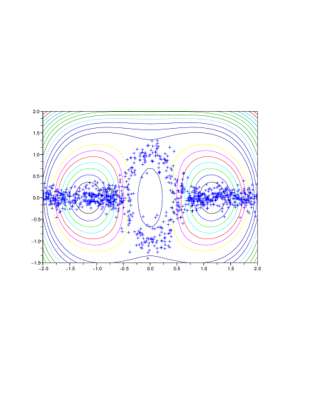
and extended periodically in the direction with period . The level sets of are depicted on Figure 1.
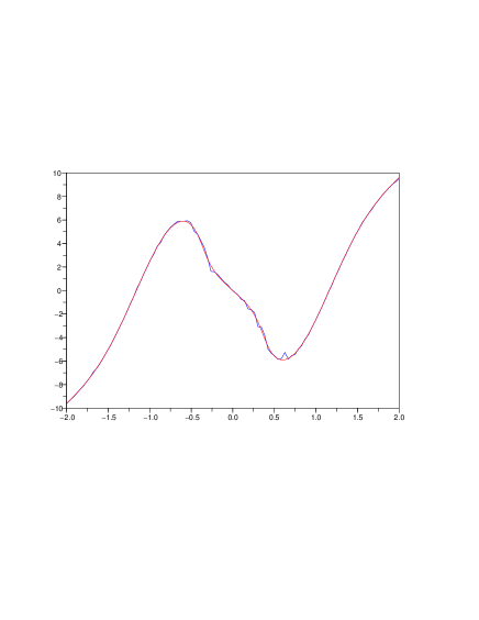
On Figure 1, we also plotted the position of the particles after iteration of an Euler-Maruyama approximation of Equation (1.3) with a time step of . The value of the parameters are , and . On Figure 2, we plotted the graph of the mean force (computed by numerical integration, which is still possible due to the low dimensionnality), and the value of the approximate mean force computed on a regular grid. The distance between the two functions is , while the norm of the function is 12.9.
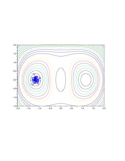
Notice that without biasing force, one obtains a very poor sampling, since the particles do not escape from the well they started in: see Figure 3, where we plotted independent simulations of a Langevin dynamics (0.1) using iterations of an Euler-Maruyama scheme of time step .
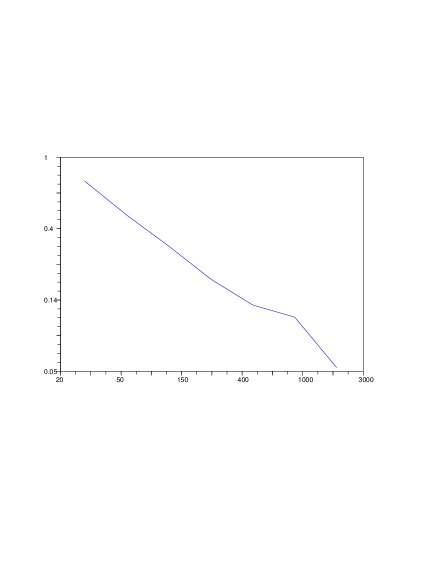
On Figure 4 we show the distance between the actual value of the mean force and its approximation at time , obtained for one simulation of the system, as a function of the number of particles used in the simulation. Using a least square regression, we find that the slope of the curve is approximatively , which matches with the theoretical rate of .
5.2 Tuning of the parameters
In Theorem 4.1, we showed that the particle approximation converges as goes to and goes to infinity, provided that does not go to zero too fast compared to . The practical difficulty that one encounters to apply this result is to choose a good scaling for in term of .
On Figure 5, we can see the error between the mean force and its aproximation at time as a function of the parameter using particles.
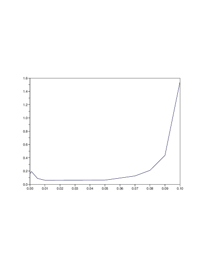
Actually, for a fixed value of , there is only a small range of values for for which the error is small.
First, the limit of the error as goes to does not even vanish as tends to infinity. The reason is that, since the particles interact with each other in a range of the number of particles which interact with a given particle is of order . Hence, when tends to while is fixed, the particles cannot see each other. Therefore, the natural limit of the particle system in the limit , fixed, should be a system of independent particles following the dynamics
Unfortunately, in the general case, the drift in the above dynamics is not obtained as the gradient of a potential, so that no invariant measure for is known. This would consequently induce a non vanishing bias in the estimation of .
For example, for the potential , one can prove that the dynamics obtained by canceling the force on the reaction coordinate , namely the couple defined by the dynamics
converges in law to the couple , where is a standard Brownian motion, is uniformly distributed on , and is a standard normal random variable, independent of . This is not the correct limit distribution, since the law of conditionned to the value of should be Gaussian, which is not the case here.
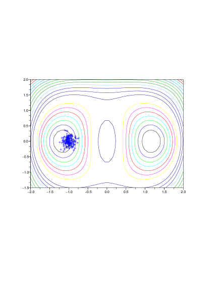
For a large value of the behavior of the particle system can be really different from the expected behavior of the dynamic (0.4). In the following example, the particles, instead of freely visiting the axis, keep stuck in the local minima they started in. Indeed, the large value of made that the biasing term is close to the mean of on all particles, whose value is close to . Consequently, the biasing force is not large enough to prevent the particle from being trapped in the local minima.
In the following example we considered the potential defined in (5.1), took , and simulated particles during iterations of time step . The result can be seen on Figure 6.
5.3 Discussion on the choice of the reaction coordinate
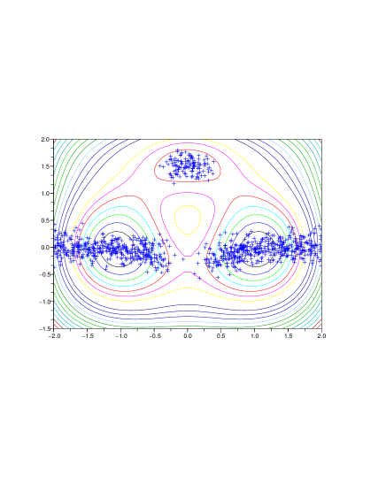
We now give another example to illustrate the limitations of the ABF method. We consider the 4-periodical potential (in the -direction) defined for in by
| (5.2) |
whose level sets are depicted on Figure 7. This potential has been introduced in [14].
The potential displays two deep minima approximately located at . There is a maximum located at , so that there are two possible paths between the main minima. The first one is a direct path meeting a saddle point approximately at . The other path goes through two saddle points at and a small minima at . Even if the first path is more direct than the second one, the prefered path in low temperature regimes will be the second one, since its energy barrier is smaller.
We simulated the particle approximation of the ABF method with particles, window width , after iterations of an Euler-Maruyama scheme of time step , and plotted the positions of the particles on Figure 7.
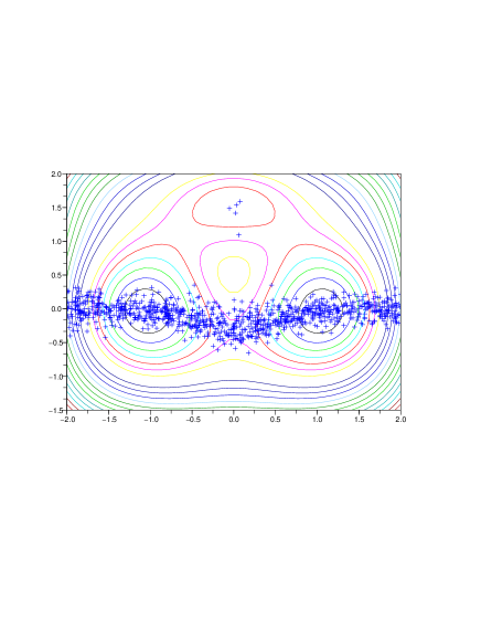
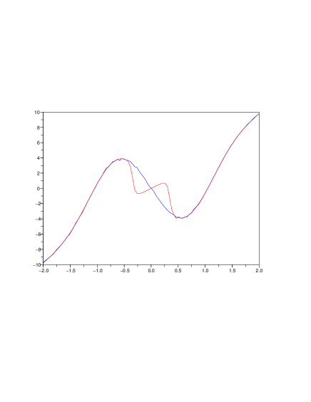
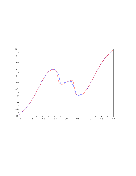
At the low temperature the particles are expected to hop from one well to the other mainly through the upper channel, which is not the case here. This is due to a bad choice of the reaction coordinate. Indeed, the biasing force only acts in the direction, so that a particle trapped in the left side well will naturally escape through a horizontal path, and will take the lower channel. As a result, the computation of the force is clearly biased, because of the poor sampling of the upper channel, see Figure 8, the distance between the two functions is of 0.4.
We still have convergence to the correct mean force, but at a slow rate, since the reaction coordinate has not been chosen in an optimal way. Indeed, with the same parameters, but after iterations, the result is much better, see Figures 9 and 10. The distance between the mean force and its approximation is of 0.15, while the function has norm 10.9.
References
- [1] R. Adams. Sobolev spaces. Academic Press, 1978.
- [2] M. Bossy, J.F. Jabir, and Talay D. On conditional McKean Lagrangian stochastic models. Preprint available at http://hal.inria.fr/inria-00345524.
- [3] H. Brézis. Analyse fonctionnelle. Théorie et applications. Collection Mathématiques appliquées pour la maîtrise. Masson, Paris, 1983. In French.
- [4] C. Chipot and A. Pohorille, editors. Free Energy Calculations, volume 86 of Springer Series in Chemical Physics. Springer, 2007.
- [5] E. Darve and A. Pohorille. Calculating free energy using average forces. J. Chem. Phys., 115:9169–9183, 2001.
- [6] R. Dautray and P.L. Lions. Mathematical Analysis and Numerical Methods for Science and Technology. Springer Verlag, 1999.
- [7] A. Dermoune. Propagation and conditional propagation of chaos for pressureless gas equations. Probab. Theor. Relat. Fields, 126:459–479, 2003.
- [8] J. Hénin and C. Chipot. Overcoming free energy barriers using unconstrained molecular dynamics simulations. J. Chem. Phys., 121:2904–2914, 2004.
- [9] N.V. Krylov and M. Röckner. Strong solutions of stochastic equations with singular time dependent drift. Probab. Theor. Relat. Fields, 131:154–196, 2005.
- [10] T. Lelièvre, M. Rousset, and G. Stoltz. Computation of free energy profiles with parallel adaptive dynamics. J. Chem. Phys, 126:134111, 2007.
- [11] T. Lelièvre, M. Rousset, and G. Stoltz. Long-time convergence of an adaptive biasing force method. Nonlinearity, 21:1155–1181, 2008.
- [12] J.L. Lions. Quelques méthodes de résolution des problèmes aux limites non-linéaires. Dunod, 1969. In French.
- [13] J.L. Lions and E. Magenes. Problèmes aux limites non homogènes et applications. Dunod, Paris, 1968-1970. In French.
- [14] P. Metzner, Ch. Schütte, and E. Vanden-Eijnden. Illustration of transition path theory on a collection of simple examples. J. Chem. Phys, 125:084110, 2006.
- [15] A.S. Sznitman. Topics in propagation of chaos. Lecture notes in mathematics, 1464, 1989.
- [16] D. Talay and O. Vaillant. A stochastic particle method with random weights for the computation of statistical solutions of McKean-Vlasov equations. Ann. Appl. Probab., 13(1):140–180, 2003.
- [17] R. Temam. Navier-Stokes equations and nonlinear functionnal analysis. North Holland, Amsterdam, 1979.
- [18] V.C. Tran. A wavelet particle approximation for McKean-Vlasov and 2D-Navier-Stokes statistical solutions. Stochastic Process. Appl., 118:284–318, 2008.
- [19] A.B. Tsybakov. Introduction à l’estimation non-paramétrique. Springer, 2004. In French.