Population Parameters of Intermediate-Age Star Clusters in the
Large Magellanic Cloud. I. NGC 1846 and its Wide Main Sequence Turnoff

Abstract

The Advanced Camera for Surveys on board the Hubble Space Telescope has been used to obtain deep, high-resolution images of the intermediate-age star cluster NGC 1846 in the Large Magellanic Cloud. We present new color-magnitude diagrams (CMDs) based on F435W, F555W, and F814W imaging. We test the previously observed broad main sequence turnoff region for ‘contamination’ by field stars and (evolved) binary star systems. We find that while these impact the number of objects in this region, none can fully account for the large color spread. Our results therefore solidify the recent finding that stars in the main sequence turnoff region of this cluster have a large spread in color which is unrelated to measurement errors or contamination by field stars, and likely due to a $\sim 300$ Myr range in the ages of cluster stars. An unbiased estimate of the stellar density distribution across the main sequence turnoff region shows that the spread is fairly continuous rather than strongly bimodal, as suggested previously. We fit the CMDs with several different sets of theoretical isochrones, and determine systematic uncertainties for population parameters when derived using any one set of isochrones. We note a degeneracy between age and [$\alpha$/Fe], which can be lifted by matching the shape (curvature) of the full red giant branch in the CMD. We find that stars in the upper part of the main sequence turnoff region are more centrally concentrated than those in any other region, including more massive red giant branch and asymptotic giant branch stars. We consider several possible formation scenarios which account for the unusual features observed in the CMD of NGC 1846.

1. Introduction

An accurate knowledge of stellar populations of “intermediate” age ($\approx$ 1 – 3 Gyr) is important within the context of several currently hot topics in astrophysics. Intermediate-age stars typically dominate the emission observed from galaxies at high redshift (e.g., van der Wel et al., 2006). Furthermore, star clusters in this age range are critical for testing predictions of the dynamical evolution of star clusters (e.g., Goudfrooij et al., 2007), and for understanding the evolution of intermediate-mass stars. The Large Magellanic Cloud (LMC) hosts a rich system of intermediate-age star clusters. The first surveys dedicated to studying properties of these clusters were based on integrated colors (e.g., Searle et al., 1980). These studies led to an empirical and homogeneous age scale based on the so-called “$S$ parameter” (Elson & Fall, 1985, 1988; Girardi et al., 1995; Pessev et al., 2008), which describes the position of the cluster in the integrated $(U\!-\!B)$ versus $(B\!-\!V)$ color-color diagram. While a number of more recent studies of such intermediate-age clusters have determined ages more directly by fitting the location of the main sequence turnoff (MSTO) region with model isochrones by means of color-magnitude diagrams (CMD; e.g., Mighell et al., 1998; Bertelli et al., 2003; Kerber et al., 2007; Mucciarelli et al., 2007; Mackey et al., 2008), such age determinations are still rather sparse and often dependent on the stellar model being used. It is important to obtain more CMD-based ages and metallicities of intermediate-age clusters and to study any systematic uncertainties related to the choice of any particular stellar model.

Mackey et al. (2008) recently used deep, HST/ACS images to study the intermediate age LMC star cluster NGC 1846 (plus two other clusters from our program GO-10595; PI: Goudfrooij). They found evidence for a wide range in turnoff colors in a fairly bimodal distribution, and concluded that these are due to two bursts of star formation separated by $\approx 0.3\times 10^{9}$ yr. Recently, a number of star clusters, primarily massive old globular clusters in the Milky Way have also been shown to have unusual color-magnitude diagrams (CMDs), suggestive of multiple stellar populations with variations in either age or abundance. This includes $\omega$ Cen (e.g., Norris et al., 1996; Hilker & Richtler, 2000; Bedin et al., 2004; Villanova et al., 2007), NGC 2808 (Piotto et al., 2007), NGC 1851 (Milone et al., 2008a), and NGC 6388 (Piotto, 2008). These globular clusters are among the most massive known in our Galaxy, and several are believed to be the remnant nuclei of stripped dwarf galaxies. NGC 1846 is roughly an order of magnitude less massive than known Galactic clusters with multiple populations, and it seems unlikely to be the stripped nucleus of a cannibalized dwarf galaxy since it is located in the outskirts of the LMC, which is a dwarf irregular galaxy itself.

In this paper we conduct a more detailed investigation of NGC 1846 in the LMC than that presented in Mackey et al. (2008), including: The effects of photometric completeness and binary star evolution, new techniques for assessing background contamination, and the radial distribution of cluster stars at different evolutionary phases. We also investigate how well different sets of isochrones and variations in [$\alpha/$Fe] fare when compared with the observations. We accomplish this by using the ePSF photometric technique (Anderson & King, 2006; Anderson et al., 2008a, b) to construct the cluster CMD, while Mackey et al. used DOLPHOT (Dolphin, 2000) for their analysis. Our results support the general conclusion of Mackey et al. (2008) that there is a large spread in the main sequence turnoff color for NGC 1846 which must be due to a range in ages, although we do find differences and additional relevant properties.

The remainder of this paper is organized as follows. § 2 presents the observations, § 3 discusses details of the stellar photometry, completeness corrections, the evaluation of contamination by field stars, and radial distributions of stars in different parts in the color-magnitude diagram of NGC 1846. § 4 presents our isochrone fitting analysis which involves different sets of theoretical isochrones, § 5 discusses the results, and § 6 presents our main conclusions.

2. Observations

NGC 1846 was observed with HST on Jan 12th, 2006, using the wide-field channel (WFC) of ACS, as part of HST program 10595 (PI: Goudfrooij). We centered the cluster on one of the two CCD chips of the ACS/WFC camera, so that the observations cover enough radial extent to study variations with cluster radius. Three exposures were taken in each of the F435W, F555W, and F814W filters: Two long exposures of 340 s each and one shorter exposure to avoid saturation of the brightest stars (90 s, 40 s, and 8 s in F435W, F555W, and F814W respectively). The two long exposures in each filter were spatially offset from each other by 3$\farcs$011 in a direction +85$\fdg$28 with respect to the positive X axis of the CCD array. This was done to move across the gap between the two ACS/WFC CCD chips, as well as to simplify the identification and removal of hot pixels.

We used two types of products provided by the HST calibration pipeline, namely the flt and drz files. The flt files have been bias corrected, dark subtracted, and flatfielded. These images are still in the WFC CCD coordinate frame, which suffers from strong geometric distortion. The drz files are composite images of exposures taken using the same filter, and are useful in the context of our analysis for two main reasons: (i) The drz files were produced using Multidrizzle (Koekemoer et al., 2003) which corrects the images for geometric distortion and ties the output image to the astrometric reference frame of the HST guide star catalog; (ii) the photometric calibration of the ACS cameras was performed on drz images (Sirianni et al., 2005, hereafter S05). On the other hand, the resampling of the images by the drizzle algorithm (Fruchter & Hook, 2002) within the Multidrizzle package makes them less suited for accurate point-spread function (PSF)-fitting photometry. Hence, we use the drz files for photometric and astrometric calibration and the flt files for measurements.

3. Analysis

3.1. Photometry

Stellar photometry was performed using PSF fitting, using the spatially variable “effective PSF” (ePSF) method described in Anderson & King (2000), and tailored for ACS/WFC data by Anderson & King (2006). A detailed description of the application of the ePSF method to ACS/WFC data is given in Anderson et al. (2008a, b). Small temporal variations of the PSF from one image to another (likely due to thermal breathing and/or small changes in the focus) were dealt with by constructing a spatially constant “perturbation” PSF for each image which was added to the library ePSF for each filter.

After fitting positions and fluxes of all stars in all individual flt images using the ePSF-fitting algorithm, they were transformed into the geometrically corrected (drz) image reference frame using the prescriptions of Anderson & King (2006). We selected all stars with the ePSF parameter “PSF fit quality” $q<0.5$ and “isolation index” of 5. The latter parameter selects stars that have no brighter neighbors within a radius of 5 pixels. To further weed out hot pixels, cosmic rays and spurious detections along diffraction spikes, the geometrically corrected positions among the three images per filter were compared. We selected objects with coordinates matching within a tolerance of 0.2 pixels in either axis, which eliminated the hot pixels and cosmic ray hits effectively. The photometry, at this stage, is given as instrumental magnitudes ($-2.5\log_{10}(\mbox{flux [e${}^{-}$]})$) for each individual exposure.

Corrections for imperfect charge transfer efficiency (CTE) of the ACS/WFC CCDs were made following Kozhurina-Platais et al. (2007), using a functional form of CTE loss that was derived from the data itself by comparing the photometry of stars from the short versus the long exposures. Using this technique, we find a different functional form for CTE loss than that published by Riess & Mack (2004). The latter was found to overcorrect the CTE loss. This difference is likely due to two main reasons: (i) The Riess & Mack (2004) correction formulae were derived from sparsely populated fields, whereas we are working with a much more crowded field. Charge traps in crowded fields are expected to be filled by charge associated with stars located at rows close to the read-out amplifier and hence the overall effective CTE loss is expected to be lower than in sparse fields (see, e.g., Goudfrooij et al., 2006); (ii) Riess & Mack (2004) performed aperture photometry on drz images, whereas we are using PSF-fitting photometry on flt files. The latter method assigns higher weights to the central pixels of stars relative to those located in the wings of the PSF, whereas aperture photometry assigns equal weights to every pixel within the aperture. The relevance of the CTE correction is illustrated in Figs. 1 and 2. The accuracy of our CTE corrections is such that the rms scatter of the magnitude residuals is 0.02 mag at an instrumental magnitude of $-2$ (corresponding to $m_{\rm F435W}$ = 23.8, $m_{\rm F555W}$ = 24.4, and $m_{\rm F814W}$ = 23.5 in magnitude units relative to Vega). This uncertainty is smaller than the photometric measurement errors at those magnitudes. After CTE correction, a final magnitude for each object was determined from a weighted average from all three available photometric measurements in a given filter. A weight of $\sigma^{-2}$ was used after rejecting saturated sources in the long exposures.

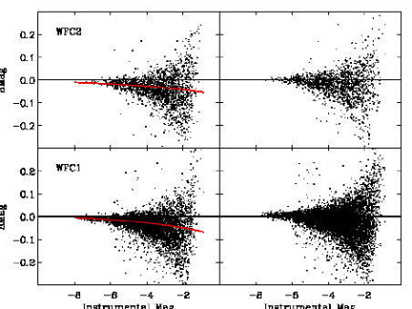
Figure 1.— The difference in normalized instrumental F435W magnitude ($-2.5$ log (e^- s^-1)) derived from short vs. long exposures as a function of normalized instrumental F435W magnitude of the long exposures. The left panels show the observed values (affected by CTE loss), whereas the right panels show the result of the CTE correction. The top and bottom panels refer to stars on the WFC2 and WFC1 chips, respectively. The overplotted solid (red online) line illustrates the average trend in magnitude residuals.

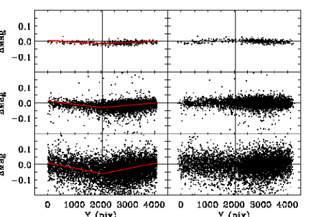
Figure 2.— The difference in normalized instrumental F435W magnitude derived from short vs. long exposures as a function of $Y$ coordinate in the drz reference frame. The left panels show the observed values (affected by CTE loss), whereas the right panels show the result of the CTE correction. The top row of panels refer to stars with normalized instrumental magnitudes $-10\leq{\rm mag}<-6$, the middle row does so for $-6\leq{\rm mag}<-4$, and the bottom row does so for $-4\leq{\rm mag}<-2$. The overplotted solid (red online) line illustrates the average trend in magnitude residuals for each chip (WFC2 for $Y\leq 2048$ and WFC1 for $Y>2048$).

3.2. Photometric Calibration

We determined final magnitudes for each star on the Vegamag photometric system following the procedure outlined in Bedin et al. (2005). Briefly, instrumental magnitudes measured with the ePSF method were compared with aperture photometry with a $0.5\arcsec$ radius of the same stars. Our final, calibrated magnitudes were then determined using:

$$m_{\rm filter}= -2.5\,\log_{10}\left(\frac{{\rm signal}\,[e^{-}]}{{\rm exptime}}\right)+{\it ZP}_{\rm filter}$$

$$-\Delta m_{0^{\prime\prime}\!\!\!.\,5-\infty}^{\rm filter}-\Delta m_{{\rm PSF}-0^{\prime\prime}\!\!\!.\,5}^{\rm filter}$$

where the subscript “filter” refers to the specific filter that was used. The first term on the right hand side is the normalized instrumental magnitude measured from the flt images using ePSF, the second term is the zeropoint from S05, the third term is the correction from 0$\farcs$5 to an infinite aperture (taken from table 1 in Bedin et al., 2005), and the fourth term is the empirically determined difference between our ePSF-fitting photometry and the aperture photometry performed for bright isolated stars in the image.

3.3. Color-Magnitude Diagrams

Figure 3.— CMDs for the HST/ACS images of NGC 1846. The top panels (a) and (b) show $m_{\rm F435W}$ vs. $m_{\rm F435W}-m_{\rm F814W}$ and $m_{\rm F555W}$ vs. $m_{\rm F555W}-m_{\rm F814W}$ for all 23,652 detected sources that passed our selection criteria. The middle panels (c) and (d) do so for a region at radii 125^′′ – 190^′′ from the center of NGC 1846 (near the corners of the HST/ACS image), and the bottom panels (e) and (f) do so for the selected sources within 25^′′ from the center of NGC 1846, a region with the same area as that shown in panels (c) and (d).

Color-magnitude diagrams (CMDs) for NGC 1846 were created for both $m_{\rm F435W}$ vs. $m_{\rm F435W}-m_{\rm F814W}$ and $m_{\rm F555W}$ vs. $m_{\rm F555W}-m_{\rm F814W}$. All stars selected as described in § 3.1 above are plotted in panels (a) and (b) of Fig. 3. To decrease contamination by field stars, we also plot CMDs including only stars within 25 arcsec from the center of NGC 1846 (which has reference pixel coordinates $(x_{c},\,y_{c})=(2225,3096)$, see § 3.5 below) in panels (c) and (d). There are several features clearly visible in the CMD of NGC 1846 shown in Fig. 3:

1. The main sequence is well defined and extends over about 6 mag in $m_{\rm F435W}$ and $m_{\rm F555W}$, and is accompanied by an obvious sequence of unresolved binary stars (running along the main sequence but slightly brightward and redward). The main sequence shows a slight change in slope near $m_{\rm F435W}$ $\approx$ 22.5, flagging the transition between radiative and convective stellar cores. Fig. 3 shows that the MSTO region is fairly wide, whereas the MS of single stars fainter than the turnoff is well-defined and much narrower (see especially panel (e)). This constitutes strong evidence for the presence of more than one population, which is discussed in more detail below.

2. The subgiant branch (SGB) is quite well defined and seems to emerge mainly from the upper end of the MSTO region.

3. The red giant branch (RGB) is well defined and quite narrow (see especially panels (a) and (e) of Fig. 3). This strongly suggests that there is little differential reddening across NGC 1846. Note that the significant width in color of the MSTO region is not reflected in the RGB. This argues that the populations that make up the MSTO share the same metallicity (in terms of [Fe/H]).

   The data allow one to clearly identify the so-called “RGB bump” at $m_{\rm F435W}$ = 20.0, $m_{\rm F435W}-m_{\rm F814W}$ = 2.1, $m_{\rm F555W}$ = 19.0, and $m_{\rm F555W}-m_{\rm F814W}$ = 1.1. This feature was first predicted by Thomas (1967) and Iben (1968), and corresponds to the period during Hydrogen shell burning when the outward-moving shell encounters extra Hydrogen fuel left behind during the period when the star had a convective envelope. The “bump” occurs as the star adjusts its structure as it consumes this extra fuel, briefly reversing its path through the CMD before resuming its ascent of the RGB (see also, e.g., Fusi Pecci et al., 1990; Denissenkov & VandenBerg, 2003).

4. The red clump (RC), sometimes called the Helium clump (since it represents core Helium burning), is located at $m_{\rm F435W}$ $\simeq$ 20.1, $m_{\rm F435W}-m_{\rm F814W}$ $\simeq$ 1.9, $m_{\rm F555W}$ $\simeq$ 19.2, and $m_{\rm F555W}-m_{\rm F814W}$ $\simeq$ 1.0.

5. The asymptotic giant branch (AGB) clump can be seen at $m_{\rm F435W}$ $\simeq$ 19.5, $m_{\rm F435W}-m_{\rm F814W}$ $\simeq$ 2.2, $m_{\rm F555W}$ $\simeq$ 18.4, and $m_{\rm F555W}-m_{\rm F814W}$ $\simeq$ 1.2. This feature corresponds to the onset of Helium shell burning.

The wide MSTO region in NGC 1846 was previously reported by Mackey & Broby Nielsen (2007) and Mackey et al. (2008), who interpreted this feature as due to the presence of two stellar populations of identical metallicity but different age. Our photometry shows some differences with that of Mackey and coworkers that potentially affects the interpretation of how this cluster formed. These differences are discussed further in § 5.

3.4. Completeness Corrections

Density distributions of stars in crowded images suffer from incompleteness. We use the standard technique of adding artificial stars to the images and running them through the photometric pipeline in order to quantify incompleteness. Specifically we use a program written by Jay Anderson (see Anderson et al., 2008a) that uses the best-fit arrays of ePSFs for each individual image, repeatedly adding artificial stars covering the magnitude and color ranges found in the CMDs. The overall radial distribution of the inserted artificial stars followed that of the stars in the image. Only 5% of the total number of stars selected in § 3.1 above were added per run, so as not to increase the degree of crowding in the images significantly. After inserting the artificial stars, the ePSF measurement and selection procedures were applied again to the image. An inserted star was considered recovered if (i) the input and output positions agreed to within 0.3 pixel, and (ii) the input and output fluxes agreed to within 0.5 mag in every filter. Completeness fractions of stars as a function of magnitude and distance from the cluster center are shown in Fig. 5 for stars in the cluster sequences, as depicted in Fig. 4.

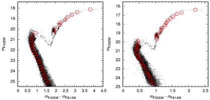
Figure 4.— CMDs of stars in regions in color-magnitude space that have less than 10% of field star contamination (see text in § 3.3). Left panel: $m_{\rm F435W}$ vs. $m_{\rm F435W}-m_{\rm F814W}$. Right panel: $m_{\rm F555W}$ vs. $m_{\rm F555W}-m_{\rm F814W}$. The open red circles in the CMDs depict the magnitudes and colors used for the completeness fractions shown in Fig. 5 (see § 3.4).

Figure 5.— The completeness fraction as function of magnitude and radius. Open squares and solid lines represent data at a radius of 5^′′, open circles and dashed lines represent data at a radius of 35^′′, and open triangles and dotted lines represent data at a radius of 125^′′. Error bars depict the standard deviations among 50 independent runs of the artificial star tests. See description in § 3.4.

Completeness fractions were assigned to every individual star in a given CMD by fitting the completeness fractions as a function $f_{\rm comp}(m,r)$ of magnitude $m$ and radius $r$:

$$f_{\rm comp}(m,r)=\frac{1}{2}\left[1-\frac{\alpha(r)\,(m-m_{\rm lim}(r))}{\sqrt{1+\alpha^{2}(r)\,(m-m_{\rm lim}(r))^{2}}}\right]$$ (1)

where $\alpha(r)$ is a free scaling parameter and $m_{\rm lim}(r)$ is the magnitude where completeness is 50%. The functional forms of both $\alpha(r)$ and $m_{\rm lim}(r)$ were chosen as third-order polynomials, fit to the data using 10 bins in radius. The overall rms of the fit to the completeness data was 0.03 for both the $m_{\rm F435W}$ vs. $m_{\rm F435W}-m_{\rm F814W}$ and the $m_{\rm F555W}$ vs. $m_{\rm F555W}-m_{\rm F814W}$ CMDs.

3.5. Radial Distributions

The wide main sequence turn-off region in NGC 1846 suggests the existence of more than one simple population. If so, it is important to find out whether the different populations have intrinsically different spatial distributions, i.e., differences beyond those that can be expected for simple (coeval) stellar populations due to dynamical evolution. A well-known example is mass segregation due to dynamical friction which slows down stars on a time scale that is inversely proportional to the mass of the star (e.g., Saslaw, 1985; Spitzer, 1987; Meylan & Heggie, 1997) so that massive stars have a more centrally concentrated distribution over time than less massive ones. With this in mind, we determined regions in the CMD that are strongly dominated by stars belonging to the cluster rather than to the underlying field in the LMC.

3.5.1 Surface Density Distribution

We first determine the projected number density of stars, taking into account the completeness corrections. The cluster center was determined to be at reference coordinate ($x_{c}$, $y_{c}$) = (2225, 3096) with an uncertainty of $\pm$ 5 pixels in either axis. This was done by creating a 2-D histogram of the pixel coordinates of stars using a bin size of $50\times 50$ pixels (i.e., 2$\farcs$5 $\times$ 2$\farcs$5), and then calculating the center using a 2-D gaussian fit to an image constructed from the surface number density values in the 2-D histogram. Note that this method avoids biases related to the presence of bright stars near the center. The ellipticity of NGC 1846 was found to be 0.12 $\pm$ 0.02, which was derived by running the task ellipse within iraf/stsdas on the surface number density image mentioned above. The area sampled by the ACS image was divided in 12 concentric elliptical annuli, centered on the cluster center. For annuli with radii larger than $\sim$ 850 pixels ($\hat{=}$ 42$\farcs$5), care was taken to account for the limited azimuthal coverage of the cluster in the image. Radii are expressed in terms of the “equivalent” radius of the ellipse, $r=a\,\sqrt{1-\epsilon}$ where $a$ is the semimajor axis of the ellipse and $\epsilon$ its ellipticity. The radial surface number density profile was fit with a King (1962) model combined with a constant background level:

$$n(r)=n_{0}\>\left(\frac{1}{\sqrt{1+(r/r_{c})^{2}}}-\frac{1}{\sqrt{1+c^{2}}}\right)^{2}\;+\;{\rm bkg}$$ (2)

where $n_{0}$ is the central surface number density, $r_{c}$ is the core radius, and $c\equiv(r_{t}/r_{c})$ is the concentration index ($r_{t}$ being the tidal radius). The best-fit King model was selected using a $\chi^{2}$ minimization routine, and is shown in Fig. 6 as well as the individual surface number density values.

Figure 6.— Radial surface density profile of NGC 1846. The points represent observed values. The dashed line represents the best-fit King model (cf. Eq. 2) whose parameters are shown in the legend.

3.5.2 Selection of Cluster-Dominated Regions on the CMD

The next step in establishing regions on the CMD that are strongly dominated by cluster stars was done statistically, by comparing star surface number densities in selection boxes on the CMD from two radial ranges: “Inner” stars with $\log(r)\leq 1.5$ versus “outer” stars with $2.0\leq\log(r)\leq 2.2$ (with radius $r$ in arcsec). Selection boxes for which the “inner/outer” surface number density ratio (after completeness correction) exceeded the value given by the best-fit King model to all stars in the ACS image were tagged as dominated by cluster stars. The selection boxes themselves were created for each evolutionary sequence in the CMD (MS, RGB, He clump, AGB), plus (bigger) boxes in the less populated areas of the CMD. For each evolutionary sequence, a ridgeline was established by means of a spline fit to carefully selected reference points along the sequence in question. After subtracting the color of the ridgeline from those of the stars in that sequence, selection boxes were divided into bins of magnitude and color. The bin size for the MS region was chosen adaptively depending on the local number density in the CMD, with a minimum of 0.2 mag in magnitude and color. For the RGB and AGB, the bin size in color was chosen to properly separate the two sequences. The selection boxes that did not correspond to the evolutionary sequences are depicted as such on Fig. 7 with dashed lines.

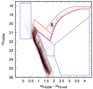
Figure 7.— A copy of Fig. 3a showing regions of interest. The red solid lines encompass regions in color-magnitude space that have less than 10% of field star contamination and for which radial distributions are shown and described in Fig. 8. The blue dashed lines encompass regions found to be heavily contaminated by field stars. See discussion in § 3.5.2.

After discarding the regions not dominated by cluster stars, we derived radial distributions of the following regions on the CMD, all of which were found to have less than 10% contamination by field stars: (i) the lower MS, meaning the MS below the turn-off of the field stars; (ii) the binary sequence associated with the lower MS; (iii) the upper MS, meaning the MS below the turn-off area but above the turn-off of the field stars; (iv) the binary sequence associated with the upper MS; (v) the ‘lower half’ of the MSTO region; (vi) the ‘upper half’ of the MSTO region; (vii) the RGB and AGB stars. Fig. 7 depicts these regions on the CMD with solid lines, while the completeness-corrected radial distributions of stars in these regions are shown in Fig. 8. Only stars with completeness fractions $\geq$ 50% were used for this exercise.

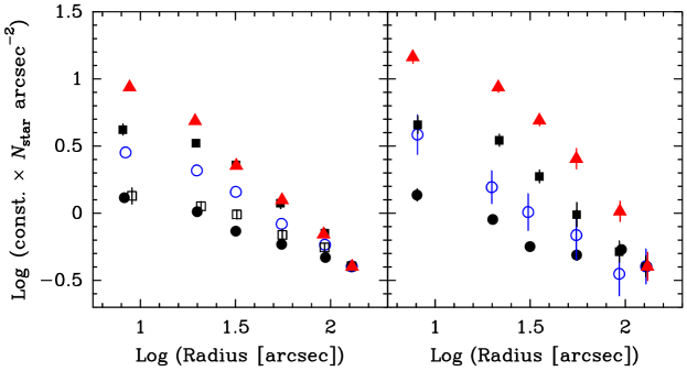
Figure 8.— Radial surface number density distributions of stars in different regions of the CMD, as depicted in Figure 7 with red solid lines. Left panel: Solid circles: all stars in the CMD. Open circles: stars in the regions of the CMD determined to have less than 10% contamination by field stars. Open squares: lower MS stars. Filled squares: upper MS stars. Filled triangles: RGB and AGB stars. Right panel: Solid circles: stars in lower binary sequence. Open circles: stars in upper binary sequence. Filled squares: lower MSTO region. Filled triangles: upper MSTO region. The absolute surface number density values on the Y axis refer to the solid circles on the left panel (“all stars”). The surface number densities of the other star types are normalized to that of “all stars” at the outermost radial bin. Error bars are only drawn if they are larger than the symbol size. See discussion in § 3.5.2.

Fig. 8 shows several items of interest. First of all, a comparison of the open squares with the filled squares in the left panel of Fig. 8 reveals that the lower MS is more heavily contaminated by field stars than the upper MS. This could have been expected given the presence of a wide turn-off near $m_{\rm F435W}$ = 23.0 and $m_{\rm F555W}$ = 22.5 (cf. Figs. 3a,b), which is clearly due to field stars. A similar effect is seen for the binary MS sequence (compare open circles with filled circles in the right panel of Fig. 8). Second, a comparison of the radial distribution of the upper MS stars with that of the bright RGB/AGB stars (filled squares and filled triangles in the left panel of Fig. 8, respectively) shows that mass segregation is not particularly strong in NGC 1846. There is a hint of the effect in the inner $\simeq$ 20″ (equivalent to $\simeq$ 5 pc), where the surface number density of RGB/AGB stars continues to rise towards the center at a slightly stronger rate than that of the upper MS stars. Last but not least, the right panel of Fig. 8 shows that the stars in the upper (brighter) half of the MSTO region are significantly more centrally concentrated in NGC 1846 than those in the lower (fainter) half of the MSTO. In fact, the stars in the upper half of the MSTO show a central concentration that is similar to (or even stronger than) that of stars in the upper RGB/AGB. The very small difference in the luminosity and mass (i.e., $\leq 5$%) of stars in the upper vs. the lower halves of the MSTO region strongly suggests that biases and mass segregation are not the cause of this difference. We conclude that the upper and lower MSTO regions correspond to intrinsically different populations which may well have undergone different amounts of violent relaxation during their collapse and/or different dynamical evolution effects. We discuss potential origins for this finding in § 5.

4. Isochrone Fitting

We fit isochrones to the CMDs of NGC 1846 to determine the age, metallicity, [$\alpha$/Fe] ratios, and their associated uncertainties. Three sets of stellar models with predictions computed for the ACS/WFC filter system were used: Padova isochrones (Marigo et al., 2008; Girardi et al., 2008), Teramo isochrones (sometimes referred to as BaSTI isochrones; Pietrinferni et al., 2004, 2006), and Dartmouth isochrones (Dotter et al., 2008).

Padova isochrones: We use the default models which involve scaled solar abundance ratios (i.e., [$\alpha$/Fe] = 0.0) and which include some degree of convective overshooting (see Girardi et al., 2000). Using the web interface of the Padova team, we construct a grid of isochrones that covers the ages $0.3\leq\tau[{\rm Gyr}]\leq 3.0$ (where $\tau$ is the age) with a step of $\Delta\tau=0.1$ Gyr and metallicities $Z$ = 0.001, 0.002, 0.004, 0.006, 0.008, 0.01, 0.02, and 0.03.

Teramo isochrones: We use that team’s web site to construct grids of isochrones that cover the same ages and metallicities as for the Padova models mentioned above. We use the Teramo isochrones with [$\alpha$/Fe] = 0.0. To allow an assessment of the influence of different amounts of convective overshooting, we construct grids for both the “canonical” models which do not include overshooting and the “non-canonical” models which do.

Dartmouth isochrones: We use the full grid available from their web site which covers the ages $0.25\leq\tau[{\rm Gyr}]\leq 1.0$ with $\Delta\tau=0.05$ Gyr and $1.0<\tau[{\rm Gyr}]\leq 5.0$ with $\Delta\tau=0.25$ Gyr, metallicities [Fe/H] = $-$2.5, $-$2.0, $-$1.5, $-$1.0, $-$0.5, 0.0, +0.3, and +0.5, and [$\alpha$/Fe] = $-$0.2, 0.0, +0.2, +0.4, +0.6, and +0.8.

4.1. Fitting Method

Isochrone fitting is performed as follows. We first establish parameters that involve pairs of fiducial points on the CMD that are: (i) relatively easy to measure or determine from both the data and the isochrone tables, (ii) sensitive to at least one population parameter such as age or metallicity, and (iii) independent on the distance and foreground reddening of the cluster. This allows us to reduce the large number of free parameters, which is always a concern when fitting isochrones to cluster CMDs. After extensive experimentation, we select the following parameters:

1. The difference in magnitude between the MSTO and the RGB bump, defined as $\Delta B_{\rm RGBB}^{\rm MSTO}$ and $\Delta V_{\rm RGBB}^{\rm MSTO}$ in the $B$ and $V$ filters, respectively. The MSTO is defined as the point where a polynomial fit to the stars (or the isochrone entries) near the turn-off is vertical in the CMD. For the location of the RGB bump on the CMD we simply calculate the mean magnitude and color of stars in a box centered on the RGB bump by eye. For the isochrones, we define the location of the RGB bump as the average of the magnitudes and colors of isochrone RGB entries between the two masses at which the magnitudes and colors “turn around” in direction on the CMD with increasing stellar mass.

2. The difference in color between the MSTO and the RGB bump, defined as $\Delta(B-I)_{\rm RGBB}^{\rm MSTO}$ and $\Delta(V-I)_{\rm RGBB}^{\rm MSTO}$.

3. The slope of the RGB. This was evaluated using the (mean) color of the RGB stars at two fiducial magnitudes, namely at $m_{\rm RGBB}+1$ and $m_{\rm RGBB}-0.75$. The former magnitude was chosen to represent a point intermediate between the RGB bump and the lower end of the RGB; the latter magnitude was chosen to avoid issues related to confusing RGB with AGB stars on the CMD. The mean colors of the RGB stars were derived from the CMD by means of a polynomial fit to the RGB star positions in the CMD. In case of the isochrones, the colors were derived by means of linear interpolation between isochrone table entries.

Figure 9.— Dependence of three distance– and reddening-independent parameters involving fiducial points on the $m_{\rm F435W}$ vs. $m_{\rm F435W}-m_{\rm F814W}$ CMD on age and metallicity for the Padova isochrones (Marigo et al., 2008). Top panels: Slope of the RGB as defined in § 4.1. Middle panels: $B_{\rm RGBB}-B_{\rm MSTO}$. Bottom panels: $(B-I)_{\rm RGBB}-(B-I)_{\rm MSTO}$. Error bars in the left and right panels reflect the variation of the parameter values among the isochrones with different metallicities and ages, respectively. The dashed lines in each panel represent the measurements of these parameters on the CMD. The upper and lower dashed lines in the middle and bottom panels refer to the upper and lower halves of the MSTO region, respectively.

Figure 10.— Same as Fig. 9, but now for the Teramo isochrones (Pietrinferni et al., 2004). The filled circles refer to the isochrones with convective overshooting, while the open circles refer to those without.

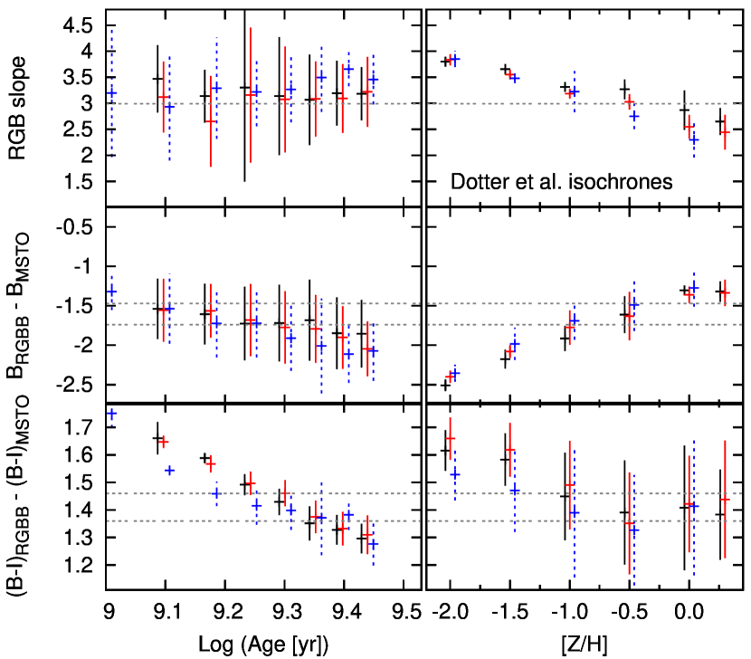
Figure 11.— Same as Fig. 9, but now for the Dartmouth isochrones (Dotter et al., 2008). The black symbols refer to the isochrones with [$\alpha$/Fe] = 0.0, the red symbols do so for [$\alpha$/Fe] = +0.2, and the blue symbols do so for [$\alpha$/Fe] = +0.6. The three sets of symbols are plotted with small relative offsets in the $x$ direction to enhance clarity; the red symbols are plotted at the correct ages and [Fe/H] values.

The sensitivity of these parameters to population parameters is illustrated in Figs. 9 – 11 for the age range 1 – 3 Gyr. These plots show the measurements of $\Delta B_{\rm RGBB}^{\rm MSTO}$, $\Delta(B-I)_{\rm RGBB}^{\rm MSTO}$, and the RGB slope as functions of age and metallicity (and [$\alpha$/Fe] in case of the Dartmouth isochrones) for isochrones in a given family, compared to the values measured in the CMD of NGC 1846. As might have been expected, the RGB slope is highly sensitive to metallicity and almost independent of age in the age range studied here. Figs. 9 – 11 also show that $\Delta B_{\rm RGBB}^{\rm MSTO}$ is dependent on both age and [Fe/H], and that $\Delta(B-I)_{\rm RGBB}^{\rm MSTO}$ is primarily dependent on age, although there are also dependences on metallicity and [$\alpha$/Fe] (see Fig. 11 for the latter) among metallicities [Fe/H] $\lesssim-1.0$ (the exact value of [Fe/H] depending on the isochrone family used).

We then select all isochrones (within each family) for which the values of these three parameters lie within 2 $\sigma$ of the measurement uncertainty of those parameters on the CMDs. This yielded 6 – 15 isochrones depending on the isochrone family. For these isochrones, we then find the best-fit values for distance $(m-M)_{0}$ and foreground reddening $A_{V}$ by means of a least squares fitting program that runs through a grid of $(m-M)_{0}$ and $A_{V}$ values to compare the magnitudes and colors of the MSTO and the RGB bump of NGC 1846 with those measured from the isochrones. The grid encompasses $18.0\leq(m-M)_{0}\leq 19.0$ with a step of 0.01 mag and $0.0\leq A_{V}\leq 0.5$ with a step of 0.01 mag. For the reddening we use $A_{\rm F435W}=1.351\,A_{V}$, $A_{\rm F555W}=1.026\,A_{V}$, and $A_{\rm F814W}=0.586\,A_{V}$. These values were derived using the ACS/WFC filter curves available in the synphot package of stsdas and the reddening law of Cardelli et al. (1989) assuming $R_{V}=3.1$. The resulting values of $(m-M)_{0}$ and $A_{V}$ derived from the positions of the MSTO and RGB bump are averaged using inverse variance weights.

 

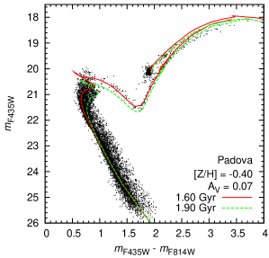
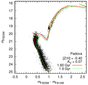
Figure 12.— Best-fit isochrones from the Padova family (cf. Table 1) superposed onto the CMDs shown in Fig. 4. The solid line is the best fit to the upper half of the MSTO region, while the dashed line is the best fit to the lower half of the MSTO region.

 

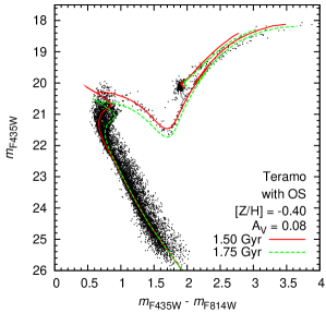
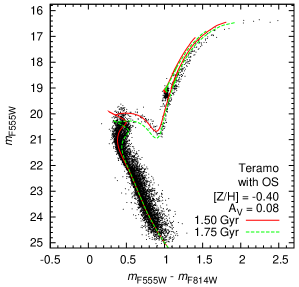
Figure 13.— Same as Fig. 12, but now for the Teramo isochrones that include convective overshooting.

 

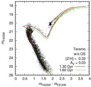
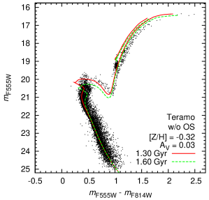
Figure 14.— Same as Fig. 12, but now for the Teramo isochrones that do not include convective overshooting.

 

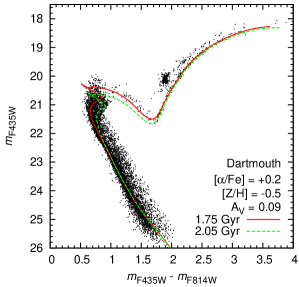
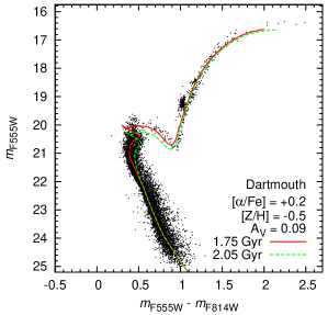
Figure 15.— Same as Fig. 12, but now for the Dartmouth isochrones.

Finally, the isochrones were overplotted onto the CMDs for visual examination. This revealed that there was a small but systematic offset in [Fe/H] between the best-fit isochrones for $m_{\rm F435W}$ vs. $m_{\rm F435W}-m_{\rm F814W}$  and $m_{\rm F555W}$ vs. $m_{\rm F555W}-m_{\rm F814W}$ in the sense that [Fe/H] was always higher for the isochrone fit to $m_{\rm F555W}$ vs. $m_{\rm F555W}-m_{\rm F814W}$ than to $m_{\rm F435W}$ vs. $m_{\rm F435W}-m_{\rm F814W}$. This effect was present for all isochrone families used, although it was least significant for the Dartmouth isochrones where the same [Fe/H]  yielded the best fit to both CMDs; in the latter case the visual check merely showed a slight mismatch of the RGB on the $m_{\rm F555W}$ vs. $m_{\rm F555W}-m_{\rm F814W}$ CMD (see Fig. 15). We suggest that it is likely that this effect is related to the fact that Kurucz model spectra of cool RGB stars contain more flux in the range $\sim$ 5000 – 6500 Å (including much of the $V$ band) than empirical star spectra from the Pickles (1998) library at the same stellar type, as recently reported by Maraston et al. (2008, and private communication). Model SEDs therefore have bluer $V\!-\!I$ colors than observed for RGB stars, consistent with what we see (see Figs. 12 – 15). While a detailed investigation of the potential cause(s) of this effect is beyond the scope of this paper, we note that the Dartmouth isochrones used the Phoenix model atmospheres (e.g., Hauschildt et al., 1999) to derive their $T_{\rm eff}$ – color relations, whereas the Padova and Teramo isochrones used the ATLAS9 models of R. L. Kurucz (e.g., Castelli & Kurucz, 2003). The use of different model atmospheres can at least partly explain this effect since the Phoenix models include 550 million molecular transitions, while the ATLAS9 models only include a few molecular lines in a semi-empirical manner. For example, the molecular band of MgH near 5175 Å which is in the $V$ band and strong in cool stars is not included in the ATLAS9 models. Because of this effect, we focus on the $m_{\rm F435W}$ vs. $m_{\rm F435W}-m_{\rm F814W}$ CMD in terms of deriving population parameters and use the $m_{\rm F555W}$ vs. $m_{\rm F555W}-m_{\rm F814W}$ CMD mainly for comparison purposes during the remaining analysis.

In order to find the difference or spread in age that can explain the wide morphology of the MSTO region of NGC 1846, the fitting process mentioned above was conducted separately for the MSTO’s measured from the upper and the lower halves of the MSTO region. During this process, we noticed that the age step $\Delta\tau$ = 0.25 Gyr used for the grid of Dartmouth isochrones is too coarse for this purpose. Hence, we created additional Dartmouth isochrones covering a finer grid in age and metallicity around the values found by the procedure mentioned above, using the web interface of the Dartmouth team web site.

The best-fit isochrones and their population parameters (both for the upper and the lower half of the MSTO region) are shown in Figs. 12 – 15, superposed onto the CMDs. While the best-fit isochrones of each model family generally match the various stellar sequences well, there are some differences between the model families. One such difference among the fits is seen in the MSTO region, where the Teramo model without overshooting provides a poorer fit than the other three models (which all do incorporate some level of overshooting). This is briefly discussed in § 4.2 below. Another, more significant difference among the isochrone fits is seen on the upper RGB, where the Padova and Teramo isochrones appear bluer than the observed stars whereas the Dartmouth isochrone is an excellent fit to the full RGB. This difference is further discussed in § 4.3 below.

Table 1Best-fit ages, metallicities, distances, reddening values, and [$\alpha$/Fe] ratio for NGC 1846 using different isochrone families. See discussion in § 4.1 and 4.4.

Isochrone	Age	Age	[Fe/H]	[$\alpha$/Fe]	$(m-M)_{0}$	$A_{V}$	rms error
Family	(upper)	(lower)					(upper)	(lower)
Padova	$1.60\pm 0.03$	$1.90\pm 0.03$	$-0.40\pm 0.05$	(0.0)	$18.42\pm 0.02$	$0.07\pm 0.02$	0.04	0.06
Teramo w/ OS	$1.50\pm 0.03$	$1.75\pm 0.03$	$-0.40\pm 0.05$	(0.0)	$18.50\pm 0.02$	$0.08\pm 0.01$	0.07	0.03
Teramo w/o OS	$1.30\pm 0.05$	$1.60\pm 0.05$	$-0.32\pm 0.05$	(0.0)	$18.43\pm 0.02$	$0.03\pm 0.02$	0.03	0.02
Dartmouth	$1.75\pm 0.03$	$2.05\pm 0.03$	$-0.50\pm 0.05$	$+0.2\pm 0.1$	$18.41\pm 0.02$	$0.09\pm 0.02$	0.02	0.02
Dartmouth	$1.95\pm 0.03$	$2.25\pm 0.03$	$-0.47\pm 0.05$	(0.0)	$18.40\pm 0.02$	$0.11\pm 0.02$	0.03	0.03
Adopted Values	$1.7\pm 0.2$	$2.0\pm 0.2$	$-0.5\pm 0.1$	$+0.2\pm 0.1$	$18.45\pm 0.05$	$0.09\pm 0.03$

The population parameters of the best-fit isochrones are listed in Table 1 for each isochrone family. Table 1 also lists the final adopted parameters for NGC 1846, including their uncertainties that reflect both errors associated with the isochrone fitting and systematic uncertainties related to the use of the different stellar models. The latter are discussed further in § 4.4 below.

4.2. Influence of Overshooting Parameter

Table 1 shows that the inclusion of convective overshooting in isochrone models in the age range appropriate for GCs like NGC 1846 has a significant effect on the derived age and [Fe/H]. In the case of the Teramo isochrones, the inclusion of overshooting results in an increase in the derived age of $\simeq$ 15% and a decrease in the derived [Fe/H] of $\simeq$ 17%.

Focusing on the morphology of the MSTO region in the CMDs, a comparison of the behavior of the best-fit Teramo isochrones that include overshooting with those that do not (see Figs. 13 and 14) suggests that overshooting is occurring in NGC 1846. Hence we do not use the parameters of the best-fit Teramo isochrones that do not include overshooting in evaluating the final adopted values of the population parameters of NGC 1846.

4.3. Influence of [$\alpha$/Fe] Abundance Ratio

We assess the influence of non-solar [$\alpha$/Fe] abundances on the derived age and metallicity by comparing our CMD with Dartmouth ischrones for different values of [$\alpha$/Fe]. The result is illustrated in Fig. 16, which shows the best-fit Dartmouth isochrones for [$\alpha$/Fe] = $-$0.2, 0.0, +0.2, and +0.4 superposed onto the $m_{\rm F435W}$ vs. $m_{\rm F435W}-m_{\rm F814W}$ CMD of NGC 1846. The fits were done to the upper half of the MSTO region in this case. Note that all four isochrones fit the MSTO and RGB bump locations well, which is likely due to the fitting method we used (as described above in § 4). However, the detailed fits along the RGB differ significantly from one [$\alpha$/Fe] value to another. In particular, there is a clear correlation between [$\alpha$/Fe] and the slope or the curvature of the RGB in the sense that larger [$\alpha$/Fe]  values give ‘flatter’ slopes and stronger curvature for the RGB.

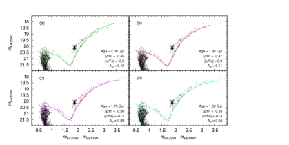
Figure 16.— Illustration of the effect of the [$\alpha$/Fe] ratio on the isochrone morphology along the RGB as well as the derived ages and [Fe/H] values. Panels (a) through (d) show the best-fit Dartmouth isochrones for [$\alpha$/Fe] = $-$0.2, 0.0, +0.2, and +0.4 respectively. The legend lists the population properties of the isochrone shown in each panel. Note the significant effect of the [$\alpha$/Fe] ratio on the slope and curvature of the RGB, as well on the resulting age and [Fe/H].

Furthermore, this comparison shows that larger values of [$\alpha$/Fe] result in younger fitted ages, and hence there is a degeneracy between age and [$\alpha$/Fe] if one doesn’t take the detailed morphology of the RGB into account. The amplitude of this effect is roughly 20% in age for a difference in [$\alpha$/Fe] of 0.2 dex (see Fig. 16). Finally, note that the effect of the chosen value of [$\alpha$/Fe] to the best-fit [Fe/H] is small within the context of our fitting procedure: $\Delta$ [Fe/H]/$\Delta$ [$\alpha$/Fe] $\simeq$ $-$0.15. Note however that the effect of non-solar [$\alpha$/Fe] to determinations of [Fe/H] can be significantly larger for analyses that aim to determine [Fe/H] values for more distant stellar systems where only the upper end of the RGB is available for isochrone fitting. This effect will be quantified in detail in a separate paper.

As Fig. 16 shows, the best fit to the full RGB is achieved using the isochrone with [$\alpha$/Fe] = +0.2. Since this fit is clearly better than any isochrone that uses solar abundance ratios in any of the three families, we adopt [$\alpha$/Fe] = +0.2 for NGC 1846.

4.4. Systematic Uncertainties in Derived Properties

We quantify systematic uncertainties in derived age, [Fe/H], distance, and reddening by comparing our best-fit results from each set of isochrones with convective overshooting and [$\alpha$/Fe] = 0.0, as compiled in Table 1. These results give systematic uncertainties of: $\pm$ 0.24 Gyr in age ($\simeq$ 15%), $\pm$ 0.05 dex in [Fe/H] ($\simeq$ 12%), $\pm$ 0.05 mag in $(m-M)_{0}$ ($\simeq$ 5% in linear distance), and $\pm$ 0.03 mag in $A_{V}$ ($\simeq$ 30%). We suggest that these values represent typical systematic uncertainties associated with the determination of population parameters of intermediate-age star clusters from $m_{\rm F435W}$ vs. $m_{\rm F435W}-m_{\rm F814W}$ CMD fitting by isochrones of any given stellar model.

Finally, we note that the properties of the best-fit isochrones are consistent with an estimate of the mass of AGB stars in NGC 1846 as derived from their pulsational properties: Lebzelter & Wood (2007) estimated ${\cal{M}}_{\rm AGB}\simeq 1.8\;\mbox{M}_{\odot}$ with an uncertainty of $\simeq 0.2\;\mbox{M}_{\odot}$ (Lebzelter, private communication). The formal AGB star masses for the best-fit isochrones in Table 1 all fall between 1.70 and 1.77 M_⊙, consistent with the independent estimate of Lebzelter & Wood.

5. Discussion

5.1. Morphology of the MSTO Region

As already mentioned in §§ 3.3 and 3.5.2, the MSTO region is broader than can be explained by photometric errors, and the upper (brighter) MSTO region has a significantly more centrally concentrated radial distribution than the lower one. This finding strongly suggests the presence of multiple (at least two) stellar populations in NGC 1846. To constrain this picture further in terms of whether or not two distinct populations are sufficient (or necessary) to produce the observed CMD, we conduct simulations of a synthetic cluster with the properties implied by the isochrone fitting in § 4. For this purpose we define the null hypothesis such that the upper and lower halves of the MSTO region represent two distinct simple stellar populations with properties given in Table 1 for the best-fit Dartmouth isochrones.

We simulate a simple stellar population (SSP) with a given age and chemical composition by populating an isochrone with stars randomly drawn from a Salpeter mass function between 0.1 M_⊙ and the RGB-tip mass, which is at 1.62 M_⊙ for the best-fit Dartmouth isochrone (see 4th entry of Table 1). The total number of stars is normalized to the observed number of stars brighter than the 50% completeness limit. To a fraction of this sample of stars we add unresolved secondary binary components that are drawn from the same mass function, hence assuming a flat primary-to-secondary mass ratio distribution for binary stars. We note that, although we are primarily investigating the morphology of the MSTO region, we fully model the stellar evolution until the onset of He-shell burning and also add secondary binary components that were evolved past the tip of the RGB. Their evolution is modeled using the He-core burning evolutionary tracks assuming an average mass-loss of 0.15 M_⊙ along the RGB and a stellar mass dispersion on the zero-age horizontal branch of 0.06 M_⊙ (see Lee, 1991; Dotter, 2008, for details). We use the width of the upper main sequence, i.e. the part brighter than the the turn-off of the background stellar population, to fix the binary star fraction at 15%. We estimate the internal systematic uncertainty in binary fraction to $\pm 5\%$ and defer a more detailed discussion of the parameter degeneracies, in particular binarity vs. mass fractions of stellar generations (i.e., the star formation history of the cluster), to a future paper. For the purposes of this work the results don’t change significantly within $\sim\!10\%$ of the binary fraction. Finally, we add photometric errors that are modeled using the distribution of photometric uncertainties of our observations to the sample of artificial stars.

We compare the observed MSTO morphology of NGC 1846 with those of the simulated CMDs by constructing a parallelogram in the CMD with the following characteristics: (i) One axis is approximately parallel to both isochrones, (ii) the other axis is approximately perpendicular to both isochrones, and (iii) it is located in a region of the MSTO where the split between the two isochrones is relatively evident. The comparison between data and simulations is then done by transforming the ($m_{\rm F435W}-m_{\rm F814W}$, $m_{\rm F435W}$) coordinates of the stars in the CMD into the reference coordinate frame defined by the two axes of the parallelogram, and then considering the distributions of reference coordinates of the stars in the direction perpendicular to the isochrones.

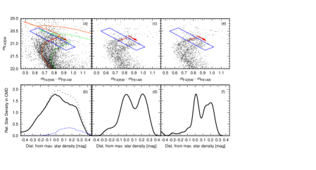
Figure 17.— Panel (a): Enlargement of the CMD shown in Fig. 3a focusing on the MSTO region. The orange and green curves represent the best-fit Dartmouth isochrones to the upper and lower halves of the MSTO region, as shown in Fig. 15. Panel (b): Distribution of stars in the parallelogram shown in the top panel, derived using a non-parametric density estimator (see text for details). The black dashed line represents all stars, the blue dashed line represents stars in the background area (scaled to the full area of the ACS image), and the solid line represents “all stars minus background”. The red arrow in panel (a) indicates the positive direction of the X axis of panel (b), while the red line indicates its zero point. Panels (c) and (d): Same as panels (a) and (b), respectively, but for the simulation of two SSPs including binary stars as described in § 5.1, with 50% of the stars belonging to the 1.75 Gyr old SSP. Panels (e) and (f): Same as panels (c) and (d), respectively, but now for the case where 60% of the stars belong to the 1.75 Gyr old SSP.

The procedure mentioned above is illustrated in Fig. 17. The top panels (a, c, and e) show the CMDs of the data and two simulations with relevant fractions of stars in the two distinct SSPs (in black dots) along with the isochrones (in orange and green) and the parallelogram mentioned above (in blue, with the reference axis along the isochrones in red). The bottom panels (b, d, and f) show the distributions of the stars’ coordinates in the direction perpendicular to the isochrones for the CMDs shown in the corresponding top panels. To avoid issues related to the use of finite histogram bin sizes in the presence of relatively few data points, the coordinate distributions were calculated by means of the non-parametric Epanechnikov-kernel probability density function (Silverman, 1986) for all objects in the parallelograms. In the case of the observed CMD (i.e., panels a and b), this was done both for stars within a radius of 42$\farcs$5 from the cluster center and for the “background region” for which the CMD was shown in Fig. 3e. The area of the probability density function of the background region was then scaled to that of the inner 42$\farcs$5 radius by area on the ACS image, and the true probability density function of the inner 42$\farcs$5 radius was derived by statistical subtraction of the background region (see panel b).

As panel (b) of Fig. 17 shows, the distribution of observed stars in the parallelogram peaks at the location of the “younger” isochrone and then declines more or less uniformly towards higher coordinate values, i.e., older ages. A comparison with panels (d) and (f) shows that the distribution of the observed stars is clearly more uniform than those of the two-SSP simulations. Two-sample Kolmogorov-Smirnov (K-S) tests confirm this visual impression: The $p$ values of the K-S tests to compare the distribution of the simulated CMDs of two SSPs with various mass fractions of the younger population against the data never exceed 11% (see Table 2). It thus seems fair to conclude from these data that the observed CMD of NGC 1846 can be better explained by a population with a distribution of ages rather than by two discrete SSPs as suggested by Mackey et al. (2008) and Milone et al. (2008b).

Table 2Results of two-sample Kolmogorov-Smirnov tests regarding the morphology of the MSTO region. Null hypothesis is that the data of NGC 1846 and the two-SSP simulations listed in the table are drawn from the same parent distribution. See discussion in § 5.1.

$f_{1.75{\it Gyr}}$	$p$ value	$f_{1.75{\it Gyr}}$	$p$ value
0.25	0.01	0.55	0.11
0.30	0.01	0.60	0.11
0.35	0.06	0.65	0.04
0.40	0.10	0.70	0.03
0.45	0.11	0.75	0.01
0.50	0.11

5.2. On The Formation of NGC 1846

The results described above naturally raise the question: How did an intermediate-age star cluster like NGC 1846 with its wide MSTO form? Is its formation related in some way to the ancient globular clusters in our own Galaxy for which evidence suggests the presence of multiple stellar populations? Based on the results of the experiments described above, we assume that the wide MSTO in NGC 1846 is due to a spread in the ages of stars found within this cluster. There are two general situations which can lead to the presence of stars with a wide range of ages within a single cluster: one involving stars which formed originally outside of the cluster and then were accreted in some way, and another where stars formed over an extended period within the cluster itself.

Three specific scenarios have been proposed for an external origin of stars with unusual CMDs: (i) the merger of two (or more) star clusters, (ii) the merger of a star cluster with a giant molecular cloud (hereafter GMC), and (iii) the entrapment of pre-existing field stars during cluster formation. As to the possibility that NGC 1846 resulted from the merger of two star clusters, the LMC is known to host tens of young (10⁷ – 10⁸ yr old) candidate double star clusters (e.g., Bhatia & Hatzidimitriou, 1988), many of which have been shown to be physically linked objects (e.g., Leon et al., 1999). On the other hand, most formation scenarios (Fujimoto & Kumai, 1997; Theis, 2002) suggest that binary clusters form within $\approx 10$ Myr, much faster than the age range seen within NGC 1846. However, it has been suggested (Mackey & Broby Nielsen, 2007) that star clusters which form in groups (star cluster groups or SCGs, see Leon et al., 1999) inside GMCs can have ages separated by a longer period of time. This idea seems consistent with the finding of Efremov & Elmegreen (1998) that the average age difference between pairs of star clusters in the LMC increases systematically with their (deprojected) angular separations, suggesting that the star formation process is hierarchical in space and time, i.e., that larger star-forming regions form stars over longer periods than small regions. However, the very small star-to-star variation in [Fe/H] in NGC 1846 allowed by the narrowness of its RGB seems difficult to account for in this scenario: Fig. 1 of Efremov & Elmegreen (1998) shows that an average age difference between star cluster pairs of $\simeq$ 200 Myr corresponds to angular separations $\gtrsim$ 0$\fdg$2, or $\gtrsim$ 150 pc at the distance of the LMC. This size is larger than that of any GMC found in the Galactic surveys reviewed in Efremov & Elmegreen (1998). Coupled with our finding above that the main sequence turnoff region in NGC 1846 does not appear bimodal as much as it appears continuous, a binary cluster merger origin for this cluster seems unlikely.

Recent simulations of mergers of star clusters with GMCs showed that such mergers can form a second-generation of stars that is (at least initially) more centrally concentrated than the first generation of stars (Bekki & Mackey, 2009), which is consistent with what we find in NGC 1846. However, to reproduce the observed features in intermediate-age star clusters with broad MSTO regions, this scenario seems to require rather strongly constrained ranges of GMC parameters such as their spatial distribution, mass function, dynamics, and chemical composition at the time the mergers would have occurred. For example, all currently known star clusters in the LMC with broad MSTO regions exhibit a range in age of $\sim 1-3\times 10^{8}$ yr (cf. Mackey et al., 2008; Milone et al., 2008b). Larger age differences have so far not been found. This would require significant fine-tuning of the range of distances between the GMCs and the initial star clusters to be merged and/or their relative velocities, whereas the current locations of the star clusters with broad MSTO regions cover a rather wide range within the LMC. Another constraint implied by this scenario is that the GMCs would all have to have the same [Fe/H] as the star clusters with which they merged, given the very small range in [Fe/H] allowed by the narrowness of the RGB in star clusters like NGC 1846.

Other simulations suggest that during formation, star clusters can trap pre-existing field stars, leading to the presence of stars with a range of ages (Fellhauer et al., 2006; Pflamm-Altenburg & Kroupa, 2007). This scenario also makes predictions which are consistent with observations: (i) the radial surface density of the trapped (older) stars will be flatter than that of stars formed in the cluster itself, and (ii) the absence of clear peaks in the distribution of stars across the MSTO region also seem compatible with this scenario. The biggest point against this scenario is that the simulations of Fellhauer et al. (2006) indicate that a star cluster with an initial mass of $\simeq$ 10⁶ M_⊙ would only be able to trap up to a few percent of its initial mass. This is inconsistent with the 30 – 40% of the stars within NGC 1846 which appear to belong to an older subpopulation. The apparent homogeneity in [Fe/H] of all stars in NGC 1846 also seems hard to explain within the field star trapping scenario.

We find that a situation where all stars formed in situ is in good agreement with several different findings for NGC 1846 noted in this paper. In particular, we suggest a scenario where gas lost by means of low-velocity winds of stars with masses lower than those producing supernovae (SN) of type II accumulates in the central regions of the star cluster and forms a second generation of stars on timescales similar to the observed age difference between the upper and lower end of the MSTO in NGC 1846. The stellar agents responsible for such self-enrichment may be (a) slow winds of fast-rotating O– and B-type stars, which occur at ages of 1 – 10 Myr (Decressin et al., 2007a) or (b) low-velocity winds of intermediate-mass ($\simeq$ 3 – 7 M_⊙) stars in the AGB phase, which have ages of 100 – 300 Myr (Ventura et al., 2001, 2002; Ventura & D’Antona, 2008). Note that the time scale for intermediate-mass AGB stars to form in the first population is similar to the actually observed age difference between the upper and lower end of the MSTO in NGC 1846. D’Ercole et al. (2008) recently performed hydrodynamical and $N$-body simulations to study the dynamical evolution of star clusters in the context of such a self-enrichment scenario. Interestingly, the D’Ercole et al. results show that clusters with masses, ages, and structural parameters similar to those of NGC 1846 are expected to show a second-generation population that is significantly more centrally concentrated than the first-generation stars (see in particular their Figure 18), just as we see in NGC 1846. This would also be consistent with the observed effect that the stars in the upper part of the MSTO are more centrally concentrated than stars in the RGB and AGB (see Fig. 8), since the latter are expected to contain stars from both populations. The slow winds from either fast-rotating massive stars or intermediate-mass AGB stars would also lead to chemical enrichment of light elements in the subsequent generation of stars due to products from the CNO cycle. If this scenario is correct, then one would expect to see significant and correlated variations in the light element abundances (e.g., C, N, O, F, Na, Mg) among the stars in NGC 1846, perhaps similarly to those found in several Galactic GCs. Measuring the chemical composition of RGB stars in NGC 1846 and other LMC clusters with wide MSTOs (e.g., Bertelli et al., 2003; Milone et al., 2008b) is feasible with current spectrographs on 8-10m-class telescopes and should provide additional relevant evidence to help decipher the most likely formation scenario.

6. Summary and Conclusions

We have used deep BVI photometry from HST/ACS images to construct CMDs of the intermediate-age star cluster NGC 1846 in the LMC. We have used the ePSF fitting technique developed by J. Anderson (Anderson & King, 2006), which returns high-accuracy photometry of cluster stars extending some 5 magnitudes below the main sequence turnoff for this cluster.

The CMD for NGC 1846 shows a number of interesting features (many of which have been noted previously): (i) a very narrow RGB; (ii) an MSTO region that is clearly broader than the (fainter) single-star main sequence; (iii) an obvious sequence of unresolved binary stars, somewhat brighter and redder than the single star main sequence. We have performed a number of new experiments, including checking the effects of background subtraction, completeness corrections, and binary star evolution, which confirm that the cluster has a statistically significant broad MSTO region.

We fit isochrones from the Padova, Teramo, and Dartmouth groups in order to determine the best-fit population parameters for NGC 1846. We perform two fits with each set of isochrones: One for the upper half of the MSTO region and one for the lower half. All three sets give a reasonably good fit to the CMD, although there are differences between the observations and predictions in the shape of the RGB for scaled-solar abundance ratios. The overall best fit to the entire CMD is achieved using the Dartmouth isochrones. The adopted parameters for NGC 1846 are: Distance $(m-M)_{0}$ = 18.45, reddening $A_{V}=0.09$, ages of 1.7 Gyr (upper half of MSTO) and 2.0 Gyr (lower half), metallicity [Fe/H] = $-$0.50, and a non-solar abundance ratio [$\alpha$/Fe] = +0.2.

We use the results from the isochrone fitting to quantify typical systematic errors of fitted population parameters for intermediate-age star clusters like NGC 1846 introduced by using any one family of isochrones, the inclusion or exclusion of convective overshooting, and the assumption of solar abundance ratios. These systematic errors are typically of order 15 – 30% for any given output parameter mentioned above.

We find for the first time that the radial distributions of stars of different masses/ages vary with statistical significance within NGC 1846, with stars in the upper MSTO (i.e., the younger stellar generation) being more centrally concentrated than stars in any other area of the CMD, including more massive RGB and AGB stars. Since this cannot be due to dynamical evolution of a simple stellar population, we conclude that the upper and lower MSTO regions correspond to intrinsically different populations which have undergone different amounts of violent relaxation during their collapse.

We have tested the role played by binary evolution on stars in the MSTO region of the CMD via Monte-Carlo simulations of multiple stellar generations. Our multi-SSP models include late stellar evolutionary stages past the He-core flash, a realistic treatment of photometric uncertainties, and a flat distribution of primary-to-secondary stellar mass ratios for binary stars. A quantitative comparison of the distribution of the stars in the MSTO region with those in the simulations that incorporate two SSPs with an age difference as indicated by the isochrone fitting shows for the first time that the observed CMD of NGC 1846 can be better explained by a population with a distribution of ages rather than by two discrete SSPs as suggested before.

Finally, we compare predictions of various formation scenarios with the observed properties of NGC 1846 described above. Scenarios where some fraction of the stars originated from outside the cluster, whether because NGC 1846 is the product of a binary cluster merger or a merger of a star cluster with a giant molecular cloud, or because the star cluster accreted older field stars during the formation process, do not appear to easily match all observed properties. A scenario where a significant fraction of the stars form later within the cluster itself out of gas enriched by stars of the earliest population(s) that feature slow stellar winds appears more consistent with the observed stellar radial density distributions and the age range implied by the width of the MSTO region. Viable sources of the enriched material are thought to include fast-rotating massive stars and intermediate-mass AGB stars. The latter have ages similar to the observed range in ages across the MSTO region. Detailed abundance ratios from high-resolution spectroscopy of individual cluster stars should be very useful in constraining the possible source(s).

Acknowledgments.

We are very grateful to Jay Anderson for his support and help in using his ePSF-related programs. We acknowledge the helpful comments and suggestions of the anonymous referee. THP gratefully acknowledges support from the National Research Council of Canada in the form of a Plaskett Research Fellowship. Support for HST Program GO-10595 was provided by NASA through a grant from the Space Telescope Science Institute, which is operated by the Association of Universities for Research in Astronomy, Inc., under NASA contract NAS5–26555. We acknowledge the use of the $R$ Language for Statistical Computing, see http://www.R-project.org.

References

- Anderson & King (2000) Anderson, J., & King, I. R. 2000, PASP, 112, 1360
- Anderson & King (2006) Anderson, J., & King, I. R. 2006, “PSFs, Photometry, and Astrometry for the ACS/WFC”, ACS Instrument Science Report 2006-01 (Baltimore:STScI)
- Anderson et al. (2008a) Anderson, J., Sarajedini, A., Bedin, L. R., King, I. R., Piotto, G., Reid, I. N., Siegel, M., Majewski, S. R., et al. 2008, AJ, 135, 2055
- Anderson et al. (2008b) Anderson, J., King, I. R., Richer, H. B., Fahlman, G. G., Hansen, B. M. S., Hurley, J., Kalirai, J. S., Rich, R. M., et al. 2008, AJ, 135, 2114
- Bastian & Goodman (2006) Bastian, N., & Goodman, S. P. 2006, MNRAS, 369, L9
- Bedin et al. (2004) Bedin, L. R., Piotto, G., Anderson, J., Cassisi, S., King, I. R., Momany, Y., & Carraro, G. 2004, ApJ, 605, L125
- Bedin et al. (2005) Bedin, L. R., Cassisi, S., Castelli, F., Piotto, G., Anderson, J., Salaris, M., Momany, Y., & Pietrinferni, A. 2005, MNRAS, 357, 1038
- Bekki & Mackey (2009) Bekki, K., & Mackey, A. D. 2009, MNRAS, doi:10.1111/j.1365-2966.2008.14320.x
- Bertelli et al. (2003) Bertelli, G., Nasi, E., Girardi, L., Chiosi, C. Zoccali, M., & Gallart, C. 2003, AJ, 125, 770
- Bhatia & Hatzidimitriou (1988) Bhatia, R., & Hatzidimitriou, D. 19
- Briley et al. (2002) Briley, M. M., Cohen. J. G., & Stetson, P. B. 2002, ApJ, 579, L17
- Briley et al. (2004) Briley, M. M., Harbeck, D., Smith, G. H., & Grebel, E. K. 2004, AJ, 127, 1588
- Bruzual & Charlot (2003) Bruzual, G. A., & Charlot, S., 2003, MNRAS, 344, 1000
- Cannon et al. (1998) Cannon, R. D., Croke, B. F. W., Bell, R. A., Hesser, J. E., & Stathakis, R. A. 1998, MNRAS, 298, 601
- Cardelli et al. (1989) Cardelli, J. A., Clayton, G. C., & Mathis, J. S. 1989, ApJ, 345, 245
- Carretta et al. (2006) Carretta, E., Bragaglia, A,. Gratton, R. G., Leone, F., Recio-Blanco, A., & Lucatello, S. 2006, A&A, 450, 523
- Castelli & Kurucz (2003) Castelli, F., & Kurucz, R. L., 2003, Modelling of Stellar Atmospheres, ed. N. Piskunov, W. W. Weiss, & D. F. Gray (San Francisco: ASP), A20
- Cohen et al. (2005) Cohen, J. G., Briley, M. M., & Stetson, P. B. 2005, AJ, 130, 1177
- Decressin et al. (2007a) Decressin, T., Meynet, G., Charbonnel, C., Prantzos, N., & Ekstróm, S. 2007a, A&A, 464, 1029
- Denissenkov & VandenBerg (2003) Denissenkov, P. A., & Vandenberg, D. A., 1003, ApJ, 593, 509
- D’Ercole et al. (2008) D’Ercole, A., Vesperini, E., D’Antona, F., McMillan, S. L. W., & Recchi, S. 2008, MNRAS, doi:10.1111/j.1365-2966.2008.13915.x
- Dolphin (2000) Dolphin, A. E. 2000, PASP, 112, 1383
- Dotter (2008) Dotter, A. 2008, ApJ, 687, L21
- Dotter et al. (2008) Dotter, A., Chaboyer, B., Jevremović, D., Kostov, V., Baron, E., & Ferguson, J. W. 2008, ApJS, 178, 89
- Efremov & Elmegreen (1998) Efremov, Y. N., & Elmegreen, B. G. 1998, MNRAS, 299, 588
- Elson & Fall (1985) Elson, R. A. W., & Fall, S. M. 1985, ApJ, 299, 211
- Elson & Fall (1988) Elson, R. A. W., & Fall, S. M. 1988, AJ, 96, 1383
- Fellhauer et al. (2006) Fellhauer, M., Kroupa, P., & Evans, N. W. 2006, MNRAS, 372, 338
- Fruchter & Hook (2002) Fruchter, A. S., & Hook, R. N. 2002, PASP, 114, 792
- Fujimoto & Kumai (1997) Fujimoto, M., & Kumai, Y. 1997, AJ, 113, 249
- Fusi Pecci et al. (1990) Fusi Pecci, F., Ferraro, F. R., Crocker, D. A., Rood, R. T., & Buonanno, R. 1990, A&A, 238, 95
- Goudfrooij et al. (2006) Goudfrooij, P., Bohlin, R. C., Maíz-Apellániz, J., & Kimble, R. A., 2006, PASP, 848, 1455
- Goudfrooij et al. (2007) Goudfrooij, P., Schweizer, F., Gilmore, D., & Whitmore, B. C. 2007, AJ, 133, 2737
- Girardi et al. (1995) Girardi, L., Chiosi, C., Bertelli, G., & Bressan, A. 1995, A&A, 298, 87
- Girardi et al. (2000) Girardi, L., Bressan, A., Bertelli, G., & Chiosi, C. 2000, A&AS, 141, 371
- Girardi et al. (2008) Girardi, L., Dalcanton, J., Williams, B., de Jong, R. S., Gallart, C., et al. 2008, PASP, 120, 583
- Gratton et al. (2001) Gratton, R. G., et al. 2001, A&A, 369, 87
- Hauschildt et al. (1999) Hauschildt, P. H., Allard, F., Ferguson, J., Baron, E., & Alexander, D. 1999b, ApJ, 525, 871
- Hilker & Richtler (2000) Hilker, M., & Richtler, T. 2000, A&A, 362, 895
- Iben (1968) Iben, I., Jr. 1968, Nature, 220, 143
- Kerber et al. (2007) Kerber, L. O., Santiago, B. X., & Brocato, E., 2007, A&A, 462, 139
- King (1962) King, I. 1962, AJ, 67, 471
- Kozhurina-Platais et al. (2007) Kozhurina-Platais, V., Goudfrooij, P., & Puzia, T. H. 2007, ACS Instrument Science Report 2007-04 (Baltimore: STScI)
- Koekemoer et al. (2003) Koekemoer, A. M., Fruchter, A. S., Hook, R. N., & Hack, W. 2003, in “2002 HST Calibration Workshop”, eds. S. Arribas, A. Koekemoer, & B. Whitmore (Baltimore: STScI), 337
- Lee (1991) Lee, Y.-W. 1991, ApJ, 373, L43
- Lebzelter & Wood (2007) Lebzelter, T., & Wood, P. R. 20076, A&A, 475, 643
- Leon et al. (1999) Leon, S., Bergond, G., & Vallenari, A., 1999, A&A, 344, 450
- Mackey & Broby Nielsen (2007) Mackey, A. D., & Broby Nielsen, P. 2007, MNRAS, 379, 151
- Mackey et al. (2008) Mackey, A. D., Broby Nielsen. P., Ferguson, A. M. N., & Richardson, J. C. 2008, ApJ, 681, L17
- Maraston (2005) Maraston, C., 2005, MNRAS, 362, 799
- Maraston et al. (2008) Maraston, C., Strömbäck, G., Thomas, D., Wake, D. A., & Nichol, D. 2008, MNRAS, 394, L107
- Marigo et al. (2008) Marigo, P., Girardi, L., Bressan, A., Groenewegen, M. A. T., Silva, L., & Granato, G. L. 2008, A&A, 482. 883
- Meylan & Heggie (1997) Meylan, G., & Heggie, D. C. 1997, A&A Rev., 8, 1
- Mighell et al. (1998) Mighell, K. J., Sarajedini, A., & French, R. S. 1998, AJ, 116, 2395
- Mucciarelli et al. (2007) Mucciarelli, A., Ferraro, F. R., Origlia, L., & Fusi Pecci, F. 2007, AJ, 133, 2053
- Milone et al. (2008a) Milone, A. P., et al. 2008a, ApJ, 673, 241
- Milone et al. (2008b) Milone, A. P., Bedin, L. R., Piotto, G., & Anderson, J. 2008b, A&A, in press (arXiv:0810.2558v1)
- Norris et al. (1996) Norris, J. E., Freeman, K. C., & Mighell, K. J. 1996, ApJ, 462, 241
- Pessev et al. (2006) Pessev, P. M., Goudfrooij, P., Puzia, T. H., & Chandar, R. 2006, AJ, 132, 781
- Pessev et al. (2008) Pessev, P. M., Goudfrooij, P., Puzia, T. H., & Chandar, R. 2008, MNRAS, 385, 1535
- Pflamm-Altenburg & Kroupa (2007) Pflamm-Altenburg, J., & Kroupa, P. 2007, MNRAS, 375, 855
- Pickles (1998) Pickles, A. J. 1998, PASP, 110, 863
- Pietrinferni et al. (2004) Pietrinferni, A., Cassisi, S., Salaris, M., & Castelli, F. 2004, ApJ, 612, 168
- Pietrinferni et al. (2006) Pietrinferni, A., Cassisi, S., Salaris, M., & Castelli, F. 2006, ApJ, 642, 797
- Piotto (2008) Piotto, G., 2008, Mem. S. A. It., 79, 3
- Piotto et al. (2007) Piotto, G., et al. 2007, ApJ, 661, L53
- Recchi & Danziger (1995) Recchi, S., & Danziger, I. J. 2005, A&A, 436, 145
- Riess & Mack (2004) Riess, A., & Mack, J. 2004, ACS Instrument Science Report 2004-06 (Baltimore: STScI)
- Saslaw (1985) Saslaw, W. C. 1985, Gravitational Physics of Stellar and Galactic Systems (Cambridge: Cambridge University Press)
- Searle et al. (1980) Searle, L., Wilkinson, A., & Bagnuolo, W. G. 1980, ApJ, 239, 803
- Silverman (1986) Silverman, B. W. 1986, in Density Estimation for Statistics and Data Analysis, Chap and Hall/CRC Press, Inc.
- Sirianni et al. (2005) Sirianni, M., Jee, M. J., Benítez, N., Blakeslee, J. P., Martel, A. R., Meurer, G., Clampin, M., De Marchi, G., et al. 2005, PASP, 117, 1049.
- Spitzer (1987) Spitzer, L. Jr. 1987, Dynamical Evolution of Globular Clusters (Princeton: Princeton University Press)
- Suntzeff & Smith (1991) Suntzeff, N. B., & Smith, V. 1991, ApJ, 381, 160
- Theis (2002) Theis, Ch. 2002, Ap&SS, 281, 97
- Thomas (1967) Thomas, H.-C. 1967, ZAp, 67, 420
- van den Bergh (2004) van den Bergh, S. 2004, AJ, 127, 897
- van der Wel et al. (2006) van der Wel, A., Franx, M., van Dokkum, P. G., Huang, J., Rix, H.-W., & Illingworth, G. D. 2006, ApJ, 2006, L21
- Ventura et al. (2001) Ventura, P., D’Antona, F., Mazzitelli, I., & Gratton, R. G. 2001, ApJ, 550, L65
- Ventura et al. (2002) Ventura, P., D’Antona, F., Mazzitelli, I. 2002, A&A, 393, 215
- Ventura & D’Antona (2008) Ventura, P., & D’Antona, F. 2008, MNRAS, 385, 2034
- Villanova et al. (2007) Villanova, S., et al. 2008, ApJ, 663, 296